STATISTICAL PROBLEMS OF TIME VARYING ...

STATISTICAL PROBLEMS OF TIME VARYING VOLATILITY IN ECONOMIC TIME SERIES Philip Messow September 2013

A DISSERTATION SUBMITTED TO THE FACULTY OF BUSINESS, ECONOMICS AND SOCIAL SCIENCES ¨ DORTMUND OF THE TECHNISCHE UNIVERSITAT

2

(Prof. Dr. Ludger Linnemann)

(Prof. Dr. Walter Krämer)

3

Acknowledgments I would like to thank to my PhD advisors, Prof. Dr. Walter Krämer and Prof. Dr. Ludger Linnemann, for supporting me during the past three years. Their ideas and sound comments helped me a lot. I would like to thank all my colleagues at Institut f¨ ur Wirtschafts- und Sozialstatistik for creating an stimulating environment within the last three years that helped me a lot finishing my thesis. This thesis was funded by the Ruhr Graduate School in Economics and I would like to thank the RGS for the financial support. I am forever grateful to my parents, Helga Thiele-Messow and J¨ urgen Messow, and my sister Marie Kristin for all their support and sympathy.

4

Contents Acknowledgments

4

1 Introduction

9

2 Historical background and motivation

12

3 Estimation of the proposed models

18

3.1

Estimation of the GARCH-model . . . . . . . . . . . . . . . . . . . . . .

18

3.2

Estimation of the APARCH-model . . . . . . . . . . . . . . . . . . . . .

20

3.3

Estimation of the ARSV-model . . . . . . . . . . . . . . . . . . . . . . .

22

4 Spurious persistence in Stochastic Volatility

29

4.1

Introduction and summary . . . . . . . . . . . . . . . . . . . . . . . . . .

30

4.2

Sample size and estimated persistence . . . . . . . . . . . . . . . . . . .

30

4.3

Structural change and empiricial autocorrelation of the logs . . . . . . . . . . . . . . . . . . . . . . . . . .

4.4 4.5

33

Structural changes and estimated persistence . . . . . . . . . . . . . . . . . . . . . . . . . . . . . . . . . . . .

34

Conclusion . . . . . . . . . . . . . . . . . . . . . . . . . . . . . . . . . . . .

35

5 Testing GARCH vs Stochastic Volatility

41

5.1

Introduction . . . . . . . . . . . . . . . . . . . . . . . . . . . . . . . . . . .

42

5.2

The models . . . . . . . . . . . . . . . . . . . . . . . . . . . . . . . . . . .

43

5.3

Testing nonnested hypotheses . . . . . . . . . . . . . . . . . . . . . . . .

44

5

5.3.1

Bootstrapped based testing . . . . . . . . . . . . . . . . . . . . .

45

5.3.2

Finite sample properties . . . . . . . . . . . . . . . . . . . . . . .

47

5.4

Empirical application . . . . . . . . . . . . . . . . . . . . . . . . . . . . .

48

5.5

Possible extensions . . . . . . . . . . . . . . . . . . . . . . . . . . . . . . .

53

5.6

Conclusion . . . . . . . . . . . . . . . . . . . . . . . . . . . . . . . . . . . .

54

6 Testing multiple volatility models

59

6.1

Introduction . . . . . . . . . . . . . . . . . . . . . . . . . . . . . . . . . . .

60

6.2

The model selection procedure . . . . . . . . . . . . . . . . . . . . . . . .

61

6.3

Models used for the simulation and empirical analysis . . . . . . . . . .

62

6.4

Simulation study . . . . . . . . . . . . . . . . . . . . . . . . . . . . . . . .

64

6.4.1

Finite sample properties . . . . . . . . . . . . . . . . . . . . . . .

66

6.5

Empirical application . . . . . . . . . . . . . . . . . . . . . . . . . . . . .

68

6.6

Conclusion . . . . . . . . . . . . . . . . . . . . . . . . . . . . . . . . . . . .

69

7 Conclusion

71

6

List of Tables 2.1

The empirical leverage effect for selected stock index returns . . . . . .

13

4.1

Impact of a structural break (0.5T) in µ on estimated persistence . . .

39

4.2

Impact of a structural break (0.5T) in ϕ on estimated persistence . . .

40

5.1

Empirical size of the C-test (DGP=GARCH-model) . . . . . . . . . . .

48

5.2

Empirical size of the C-test (DGP=SV-model) . . . . . . . . . . . . . .

48

5.3

Empirical size of the bootstrapped C-test (DGP=GARCH-model) . .

49

5.4

Empirical size of the bootstrapped C-test (DGP=SV-model) . . . . .

49

5.5

Empirical power of the bootstrapped C-test (DGP=SV-model) . . . .

49

5.6

Empirical power of the bootstrapped C-test (DGP=GARCH-model) .

50

5.7

Test statistics for selected stock index returns . . . . . . . . . . . . . .

51

5.8

Test statistics for selected exchange rate returns . . . . . . . . . . . . .

52

6.1

Empirical size of the MC-test (DGP=SV-model) . . . . . . . . . . . . .

66

6.2

Empirical size of the bootstrapped MC-test (DGP=SV-model) . . . .

67

6.3

Empirical power of the bootstrapped C-test (DGP=SV-model) . . . .

67

6.4

Selected models for the considered stock index returns . . . . . . . . .

69

7

List of Figures 2.1

DAX daily returns 05/08/1998 - 05/09/2013 . . . . . . . . . . . . . . .

3.1

Left: Comparison of the log-χ21 and the normal density (dashed); Right: Logarithm of the ratio of both densities . . . . . . . . . . . . . . . . . .

3.2

17

27

Comparison of the log of a χ21 density and the fitted normal mixture (dashed); Right: Logarithm of the ratio of both densities . . . . . . . .

28

4.1

Estimated persistence and sample size in the ARSV(1)-model . . . . .

36

4.2

Estimated persistence of the CAC 40 returns . . . . . . . . . . . . . . .

37

4.3

Rolling window estimation of persistence for the US-$ to British pound exchange rate returns . . . . . . . . . . . . . . . . . . . . . . . . . . . . .

38

5.1

Returns of selected stock indices from 11/2002 - 11/2012 . . . . . . . .

55

5.2

Distribution of the bootstrapped test statistic for the HANGSENG return series . . . . . . . . . . . . . . . . . . . . . . . . . . . . . . . . . . .

56

5.3

Returns of selected exchange rates from 05/2003 - 05/2013 . . . . . . .

57

5.4

Distribution of the bootstrapped test statistic for the Swiss Franc to

6.1

Euro return series . . . . . . . . . . . . . . . . . . . . . . . . . . . . . . .

58

Returns of selected stock indices from 11/2002 - 11/2012 . . . . . . . .

70

8

Chapter 1 Introduction Modeling the behavior of returns of speculative assets and economic quantities is one of the major fields in econometric research. Mandelbrot (1963) and Fama (1965) outlined that the distribution of these returns is non-normal and can be characterized by so-called ’stylized facts’, e.g. heteroskedasticity, the ’leverage effect’ and fatter tails than the normal distribution. These observations are in line with the ongoing financial crisis as no one would argue that volatility is time constant nor changes randomly over time. By looking at return series of the past 15-20 years one could easily observe that the volatility of these returns is dramatically fluctuating within the given time frame, but still exhibit some special patterns that are worthwhile to explore in detail. This observation describes the need for using time-varying volatility models instead of time-constant volatility models. A time-varying volatility structure can be implemented by one-shock models (Autoregressive Conditional Heteroskedastic-models) or two-shock models (Stochastic Volatility-models). Time-varying volatility models have multiple areas of application in (financial) economics. First of all, GARCH- and SV-models are widely used for volatility forecasting (but not for the returns itself). Due to the special characteristics of the return series (e.g. volatility clustering, ’leverage effect’) it is possible to forecast future volatilities reasonably well. These forecasts are used mainly by banks and insurance companies for credit risk management purposes. Compared to standard models where the conditional and unconditional variance is time-constant 9

CHAPTER 1. INTRODUCTION

10

as for example ARMA-models, risk measures as the value-at-risk or the expected shortfall are much more accurate when using time-varying volatiliy models and thus credit risks can be better controlled because these risk measures are a function of volatility. A second field of application of GARCH- and SV-models is option pricing. The price of an option is a function of the underlying asset’s volatility. Pricing of these derivates is much precise by using time-varying volatility models. Other fields of application for time-varying volatility models are the modeling of the volatility of inflation (Coulson and Robins, 1985) and the term structure of interest rates (Engle et al., 1985). The historical background of time-varying volatility models is outlined in chapter 2. Both models are the main workhorses for modeling time-varying volatility in economic time series and have a lot of characteristics in common but also some remarkable differences. There are two main differences that can be identified between both model classes. On the one hand, the economic interpretation is different for the two models. Within the one-shock models the conditional variance in period t is perfectly explained by all information at time t 1. This does not hold for the two-shock models as the additional error term reflects the random and uneven flow of information to financial markets. On the other hand the practical handling of both models is different with respect to estimation. One-shock models can be estimated with standard Maximum-Likelihood techniques. Two-shock models are much harder to estimate due to the additional error term entering the conditional volatility equation. Typical estimation techniques for two-shock models include both Bayesian approaches, as e.g. Markov-Chain-Monte-Carlo (MCMC)-methods, and non-Bayesian approaches, as e.g. Quasi-Maximum-Likelihood estimation (QMLE) or the expectation-maximization (EM)-algorithm. The estimation techniques used for my work are explained in chapter 3, focusing on the SV-model estimation. The differences of SV- and GARCH-models outlined above motivate the work of chapter 5 and 6 where a non-nested testing procedure is developed for discriminating between GARCH- and SV-models. Within chapter 5, I introduce a testing procedure that is capable of discriminating between two different models. It goes back to the popular J- and C-tests of Davidson and MacKinnon (1981). The focus of chapter 6 lies in the

CHAPTER 1. INTRODUCTION

11

extension of the testing procedure of chapter 5 for discriminating not only two but up to M different models. This type of test goes back to Hagemann (2012). Another speciality when calibrating GARCH- and SV-models to empirical data is the fact, that the estimated persistence tends to unity as sample size increases. Chapter 4 shows that this observation can be induced by structural breaks within the data generating process (DGP) and thus is not necessarily caused by a real large persistence parameter. But for SV-models, estimated persistence does not tend to unity if the sample size goes to infinity. This is different to GARCH-models where estimated persistence tends to unity if the structural break becomes more pronounced or sample size goes to infinity. Chapter 7 concludes and gives an overview how the methods introduced in chapter 4-6 could be extended for further research.

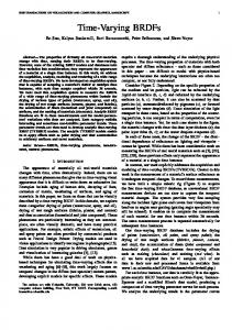
Chapter 2 Historical background and motivation As pointed out in chapter 1, the stylized fact that return series of economic quantities have fatter tails than the normal distribution were pioneered by Mandelbrot (1963) and Fama (1965). Both authors suggest the stable Paretian family of distributions for capturing the statistical properties of these return series. Further suggestions for the distribution of return series include the t-distribution (Praetz, 1972), the lognormal-normal model of Clark (1973) and a mixture of normal distributions (Kon, 1984). Boothe and Glassman (1987) compare different distributional assumptions for exchange rate returns and find out that the t-distribution and a mixture of two normal distributions provide the best fit. However, there is evidence that (some of) the distribution parameters are not constant and vary over time. This leads to a second stylized fact, namely that rates of returns for stock prices and exchange rates seem to be uncorrelated over time but are not independent. The first one pointing this certainty out was Mandelbrot (1963), as he mentioned that large changes tend to be followed by large changes in both directions and small changes tend to be followed by small changes, resulting in so-called volatility clusters. To illustrate these stylized facts, figure 2.1 shows the behavior of the DAX ranging from 05/08/1998 to 05/09/2013 and the daily (absolute) returns. The behavior of the DAX is clearly nonstationary, but the series of the daily returns exhibits stationarity with a mean 12

CHAPTER 2. HISTORICAL BACKGROUND AND MOTIVATION

13

Table 2.1: The empirical leverage effect for selected stock index returns Stock Index

DowJones

Correlation

0.029

Stock Index

DAX

CAC

FTSE

0.005

0.029

BOVESPA HANGSENG

Correlation

0.008

0.022

0.028

KOSPI

0.161

RTS

0.124

NIKKEI

0.168

TAIEX

0.148

Notes. Level of significance: ***:1%

of 0.00012. There is also a clear tendency for volatility clustering in bear markets with peaks around March 2000 (dot-com bubble) and September 2008 (recent financial crisis) which is shown by the bottom figure of 2.1 illustrating the daily absolute returns of the DAX. Another typical stylized fact observed when modeling stock (index) returns is the so-called ’leverage effect’. This stylized fact describes the asymmetric responses to negative and positive shocks, as negative shocks tend to have a higher impact on future volatility than positive shocks. If the leverage effect holds, the returns of period t 1 and the squared returns of period t are negatively correlated. This contradicts the efficient market hypothesis, because even though stock market returns have little to no serial correlation (Taylor, 1986), they are dependent. This stylized fact is often called ’Taylor-effect’ in the literature. Speaking in economic terms, information should affect the price of an asset at the arrival of the particular information. But if information is clustered for a specific time interval, the distribution of the next return depends on the previous returns, even though there is no correlation (Ding et al., 1993). Table 2.1 illustrates the ’empirical leverage effect’ for selected stock index returns. It turns out that four out of ten return series exhibit significant negative correlation, indicating that the efficient market hypothesis does not hold because otherwise if the return series is i.i.d., every transformation of it is also an i.i.d. process and thus there should be no significant correlation of the transformed return series. Engle (1982) invented the so called ’Autoregressive Conditional Heteroskedastic’ (ARCH)-model for modeling these types of dependency. Within the framework of


14

the ARCH-model, the conditional distribution of the errors is normal, but the conditional variance is a linear function of past squared innovations. Therefore large returns are more likely to be followed by large returns but the sign of the return is not predictable because of the squared values. Even though the fit of the ARCH-model is pretty good, normally a relatively high order of past innovations need to be included in the conditional variance equation. Bollerslev (1986) extends the ARCH-model to the ’Generalized Autoregressive Conditional Heteroskedastic’ (GARCH)-model including not only past squared innovations but also past realization of the conditional variance itself. Within the GARCH-framework a much more parsimonious parametrization is needed for obtaining the same results as within the ARCH-framework. The GARCH-model is still the main workhorse in financial econometrics due to its good fit and simultaneously small parametrization. One major drawback of the GARCHframework is the symmetric responses to shocks and thus it is not able to capture the ’leverage’-effect. Therefore Nelson (1991) introduced the Exponential Generalized Autoregressive Conditional Heteroskedastic (EGARCH)-model, which is capable of reproducing the ’leverage’-effect. There are several other models that are also capable of producing an asymmetric response, as for example the GJR-GARCH by Glosten et al. (1993) and the APARCH-model by Ding et al. (1993). The estimation of GARCH-models is straightforward and typically done by conditional Maximimum Likelihood estimation. There is a competing model for describing these stylized facts, the Stochastic Volatility (SV)-model. The SV-model was introduced by Taylor (1982) and differs from the GARCH-model in such a way that an additional error term enters the conditional variance equation. The behavior of these models is pretty similar to GARCH-models but with two distinct differences. On the one hand, the additional error term yields a different economic interpretation because within the GARCH-framework the volatility for t 1 is perfectly described by all information gathered at time t. Due to the additional error term this does not hold for the SV-model. The second error term can be interpreted as the random and uneven flow of information into the financial markets. On the other hand, the estimation of SV-models is not as straightforward as in the GARCH-case. Even though SV-models are not as highly used in the literature


15

for empirical applications as GARCH-models due to the simple estimation techniques of the latter ones (and thus the implementation in standard software packages), there are several extensions to the basic SV-model. For example it is also possible to reflect the ’leverage effect’ within the framework of Stochastic Volatility or to relax the normality assumption of the errors (Jaquier et al., 1999; Harvey and Shepard, 1996). These differences raise interest in discriminating between GARCH- and SV-models. The standard model selection procedure relies on nested hypothesis testing. Nested means that one of the models can be obtained from the other models by imposing parameter restrictions or by a limiting process (Pesaran and Weeks, 1999). The major disadvantage of nested hypothesis testing is that these procedures implicitly assume that one of the models is the true data generating process (DGP), because nesting two models, a representative test just checks whether a specific restriction holds or not. This approach is the traditional way of testing of two models under consideration and goes back to Kim et al. (1998). Because in most applications the SV-model is the more sophisticated one, it is often assumed that the GARCH-model is nested within the SV-model. Other popular examples are Kobayashi and Shi (2005) and Franses et al. (2008). But as stressed out by Hansen (2005), (econometric) models are just approximations to the true data generating process and thus will never fit the DGP exactly. Given this fact, the goal of a researcher is to find a good approximation to the true DGP but not finding the true DGP and hence a nested testing procedure is not appropriate and thus a specification test should be able to reject all models or accept more than one model. The problem described above can be circumvented by not asking the question ’which model is the correct one’ (nested testing) but asking ’is one of the models under consideration a good approximation to the true model’ by using a nonnested testing procedure. By doing so, the possible outcome is the following: a) All models are good approximations to the true DGP. b) One or more models are good approximations to the true DGP. c) None of the models is a good approximation to the true DGP.


16

This approach is especially fruitful for time-varying volatility models because there are countless different GARCH- and SV-models proposed in the literature and picking an appropriate one is a challenging task. Bollerslev (2008) lists more than 100 different GARCH-models in his glossary and the amount of different SV-models is not even remotely comprehensible. This confirms the need for a well working model selection technique in the field of time-varying volatility models and motivates the proposed testing procedures in section 5 and 6. When applying GARCH-models to return series it is a well known fact that persistence in these types of models tends to unity if sample size increases. From a theoretical point of view, this high persistence can be induced by structural breaks within the model parameters. Thus it is shown (Krämer et al., 2011, among others) that persistence tends to unity if the sample size goes to infinity or if the structural breaks become more pronounced. Within chapter 4 I analyze if these findings also hold for SV-models or if there are differences for these type of models.

2000 4000 6000 8000

2005

2010

2000

2005

2010

2000

2005

2010

0.04

0.08

−0.05

0.05

2000

0.00

DAX daily absolute returns

DAX daily returns

DAX daily index values


Figure 2.1: DAX daily returns 05/08/1998 - 05/09/2013

17

Chapter 3 Estimation of the proposed models This chapter derives important properties of the models used in the following chapters and explains techniques for estimating the different models. For all models, there are different estimation techniques than the proposed ones available with different benefits and drawbacks, but I will focus on the ones that were actually applied for estimating the models used in the following chapters.

3.1

Estimation of the GARCH-model

A stochastic process is called GARCH(p,q) if for yt

µt εt with εt

zt σt the following

holds: E yt Sϕt1

µt

Varyt Sϕt1

σt2 q

p

α0 Q αi yt21 Q βj σt2j j 1

i 1

with

αi C 0,

¦

i

1, ..., p 1,

αp A 0,

βj C 0,

¦

j

1, ..., q 1 and βq A 0.

18

CHAPTER 3. ESTIMATION OF THE PROPOSED MODELS

19

p

ϕt1 describes all information available at time t 1. For weak stationarity q

P αi i 1

P βj @ 1 must hold and if the disturbances are weakly stationary, then the uncondij 1 tional variance does not change over time and reads Varyt

α0 p

1 P αi i 1

q

P βj

.

j 1

Even though we assume that zt N ID0, 1 we cannot give an explicit expression of the pdf of yt because the distribution of σ1 , ..., σT is not known. To circumvent this problem we make use of a conditional Gaussian distribution and define

f εt Sϕt1

εt Sϕt1 N 0, σt2 1 ε2 º exp0.5 t2 . σt 2πσt

(3.1) (3.2)

The parameter vector of the GARCH-model is traditionally estimated by MaximumLikelihood-techniques. The conditional likelihood of ym1 , ..., yT given ϕm with m max p, q and θ α0 , ..., αp , β1 , ..., βq reads (assuming µt 0) T

Lθ

M

t m1

fθ εt Sϕt1 ,

where fθ εt Sϕt1 is the density specified in (3.2). By taking logarithms, we end up at the conditional log-likelihood (Franke et al., 2001): l θ

where we assume σ02

T

2

1

log2π

1 T 1 T εqt 1 2 log σ , Q Q t 2t 2 2 t q1 σt2

(3.3) p

0. By maximizing (3.3) we obtain estimates

q

P αî, jP1 βˆj . i 0

These estimates are consistent, asymptotically normal distributed and asymptotically efficient (Schmid and Trede, 2006). Optimization is traditionally done by applying a numerical method as for example the BFGS-algorithm.


20

It is worth noting that the likelihood tends to be flat and thus one needs a rather large T to circumvent this problem. A straightforward extension to the (standard) GARCH(p,q)-model with normally distributed innovations is to allow for conditionally t-distributed errors. Even though in the GARCH-model with conditionally normal innovations the unconditional distribution is leptokurtic (Bollerslev, 1987), empirical data is even more leptokurtic than the traditional GARCH-model can capture. So there is a need to account for this by allowing the conditional distribution of the innovations to be student’s-t. If the conditional distribution of εt

¦

t

1, ..., T given ϕt1 is student’s-t with v the degrees

of freedom εt Sϕt1 tv 0, σt2 , then the estimation is as straightforward as before by using Maximum Likelihood with the following conditional density according to Bollerslev (1987) εt Sϕt1 fv εt Sϕt1 v1 v 1 2 0.5 Γ Γ v 2σt 2 2 v A 2.

3.2

2

1 εt

σt2 v 21

v 1 2

,

Estimation of the APARCH-model

Another popular extension to the GARCH-model is the APARCH(p,q)-model pioneered by Ding et al. (1993). Within the APARCH framework the conditional variance can respond differently to positive and negative shocks of the same magnitude. Speaking in economic terms, positive and negative information regarding an asset lead to different levels of conditional variance. This pattern is called the ’leverageeffect’ and the GARCH-model is not capable of reproducing this stylized fact. As already mentioned in chapter 1, return series of economic quantities are often serial uncorrelated but not independent, because some kind of (non-linear) transformation of the return series exhibits correlation. In the literature this observation is often


21

called ’Taylor effect’ because Taylor (1986) was the first one describing this economic pattern. To account for both stylized facts, the APARCH(1,1)-model has two additional parameters compared to the GARCH(1,1)-model: yt

µt ξt

(3.4)

ξt

εt σt

(3.5)

σtϱ

χ α1

χ A 0, ϱ C 0 ,

Sξt1 S ω

α1 C 0,

ξt1 ϱ β1 σtϱ1

1 @ ω @ 1, β1 C 0.

(3.6) (3.7)

The ’leverage effect’ is introduced into the model via ω. A positive ω means that negative information has a stronger impact on volatility than positive information. ϱ reflects the ’Taylor effect’. The APARCH-model nests seven other GARCH-type models: ARCH: ϱ

2, ω

GARCH: ϱ

0 and β1

2, ω

0.

Taylor/Schwert GARCH: ϱ GJR-GARCH: ϱ

1, ω

0.

2.

TARCH: ϱ

1, β1

0.

NARCH: ω

0, β1

0.

log-ARCH: ϱ

0.

0.

The unconditional variance of εt is explained by


σt2

χ 1 α1 1 ω 2 β1

22

.

By assuming that the conditional distribution of ξt is normal ξt Sϕt1 N 0, σt2 , Maximum-Likelihood techniques can be applied for estimating the parameter vector Λ

χ,

α1 , ω, ϱ, β1 and the log-likelihood reads (assuming ϱ

2)(Laurent,

2004) l Λ

3.3

T T 1 ξ2 T log2π Q logσt2 Q t2 . 2 t 1 t 1 σt

Estimation of the ARSV-model

Due to the additional error term, estimation of the SV-model is not as straightforward as for the class of GARCH-models. The ARSV(1)-model is defined as yt

zt σt

ht

ln σt2

(3.8) γ Ξht1 ξt ,

(3.9) σ2

If SΞS @ 1, then ht is strictly stationary with mean 1γΞ and variance 1Ξξ 2 . Furthermore it is assmued that ξt N 0, σξ2 . To fully capture and understand the dynamics of the model, one may rewrite it in the form of rt since yt

log yt2

ht log zt2

(3.10)

zt exp0.5ht . By using this transformation, the model is in its state-

space form: (3.10) is the observation equation and ht is the unobserved state process. Because the state process ht is not directly observable, you want to estimate the ’signal’ of ht given the data set r1 , ..., rt . The estimation in this kind of models is normally done by using Kalman filtration. The Kalman Filter is a particular algorithm that is used to solve state space models in the linear case with normally distributed errors. This was first derived by Kalman (1960). If zt N ID0, 1, then


w

23

log zt2 is log-χ2 distributed with one degree of freedom and the density is given

by f w

1 exp 0.5expw w , ª @ w @ ª. 2π

º

(3.11)

The mean of log zt2 is -1.27 and the variance is 0.5 π 2 4.93. Harvey et al. (1994) estimate the parameter vector ψ log LQ ψ

γ, Ξ, σξ2

T log2π 0.5 2

by maximizing the log-likelihood T

Q log t 1

T

vt2 . 1 Ft

Ft 0.5 Q t

vt describes the one-step-ahead prediction error for the best linear estimator of logyt2 , Ft stands for the corresponding mean squared error and y

y1 , ..., yt .

Kim et al.

(1998) point out that this Quasi Maximum Likelihood Estimator is consistent and asymptotically normal distributed but as it turns out (and is shown in figure 3.1) logzt2 is poorly approximated by a normal distribution. As a consequence even though the asymptotic theory holds, this QMLE has poor finite sample properties. Figure 3.1 shows that both densities differ quite substantially and the difference is becoming more extreme for greater values. Shumway and Stoffer (2011) recommend to approximate logzt2 by a mixture of two normal distributed variables, where one is centered at zero. (3.10) then reads log yt2 Θt

Ψ ht Θ t It zt0 1 It zt1

with zt0 N 0, σ02 and zt1 N µ1 , σ12 . It describes an IID Bernoulli distributed variable with PIt

0

π0 and PIt

1

π1 and π0 π1

1. Figure 3.2 shows the

comparison of Θt estimated given the data of the DAX from chapter 2 and the log of a χ21 (formula (3.11)). Comparing graphic 3.1 and 3.2 one observes that the fit of the mixture of two normals to the log-χ2 density is enhanced dramatically and this model is also easy to fit due to the normality assumptions (Shumway and Stoffer, 2011). The filter equations for the proposed models are


24

1

htt1

γ Ξhtt1 Q πtj Ktj ϵtj

Ptt1

Ξ2 Ptt1 σξ2 Q πtj Ktj2 Σtj

(3.13)

zt0

log

j 0 2 t1 y t Ψ ht

(3.14)

zt1

log yt2 Ψ htt1 µ1

(3.15)

Σt0

Ptt1 σ02

(3.16)

Σt1

Ptt1 σ12 ΞPtt1 Σt0 ΞPtt1 Σt1

(3.17)

(3.12)

j 0

1

Kt0 Kt1 where hst

E ht Sr1 , ..., rs , Pts

(3.18) (3.19)

E ht hst ht hst , something similar to the mean

squared error (MSE) and Ktj the Kalman gain. Equation (3.12) and (3.13) are called the prediction equations and (3.14) and (3.15) are called the prediction errors. The corresponding variance-covariance matrices of the errors are defined in (3.16) and (3.17). The advantage of Kalman filtering is, that it specifies how to update the filter from htt11 to htt once a new observation rt is obtained, without having to reprocess the entire data set r1 , ..., rt (Shumway and Stoffer, 2011). For applying the filter one need to determine πt0 and πt1 πt0

PIt

0Sr1 , ..., rt and πt1

PIt

1 πt0 , t

1, ..., T , with

1Sr1 , ..., rt . Let fIt tSt 1 describe the

conditional density of yt given the past observations y1 , ..., yt1 , then we can define πt1

π1 f1 tSt 1 . π0 f0 tSt 1 π1 f1 tSt 1


It is reasonable to assume that π0

π1

25

0.5 and fIt tSt 1 is approximated well

enough by N htt1 µ1 , Ptj (Shumway and Stoffer, 2011). The likelihood for estimating the parameter vector Λ

γ,

log Lr1 ,...,rt Λ

Ξ, σξ , Ψ, σ0 , µ1 , σ1 reads

T

1

t 1

j 0

Q logQ πj fj tSt

1.

(3.20)

With the specification of the Kalman filter and the log-likelihood, the estimation procedure can be summarized in four steps: 1.) Initial parameters need to be chosen. The initial parameter vector I used for the estimation looks like the following: Λ0 r, σ0

1, µ1

3, σ1

γ

0, Ξ

0.95, σξ

0.2, Ψ

2 .

2.) The Kalman filter in (3.12)-(3.19) is applied by using the initial parameter values Λ0 . By doing so, errors and covariances of the errors are obtained. 3.) Apply a Quasi-Newton-Raphson algorithm, e.g. the Broyden-Fletcher-GoldfarbShanno (BFGS) method, by using (3.20) as criterion function and obtain a new set of parameter estimates Λ1 . 4.) Repeat step 2 using the new set of parameter estimates and obtain new errors and covariances of the errors. Then repeat step 3 and stop, if the difference between LΛj and LΛj 1 is small enough. In practice, it can be quite difficult to minimize (3.20) by standard optimization methods (as for example the BFGS-algorithm of ’optim’ of the programming language ’R’ mentioned above) as these methods fail to converge. If this problem occurs one need to carry out the minimization of (3.20) with more sophisticated optimization techniques as for example ’evolutionary algorithm’ based on the package ’DEoptim’ for ’R’ programming language. ’DEoptim’ is an global optimization method which uses differential evolution. Differential evolution belongs to the class of genetic algorithms which use biology-inspired operations of crossover, mutation, and selection on a population in order to minimize an objective function over the course of successive generations. This stochastic global optimization algorithm is more apt of finding a


26

global solution as gradient based methods often do not converge or converge to local minima.

27

0.0

−50

0.1

0

50

0.2

100

0.3

150

0.4


−20

−10

−5

0

5

−20

−10

−5

0

5

Figure 3.1: Left: Comparison of the log-χ21 and the normal density (dashed); Right: Logarithm of the ratio of both densities

28

0.0

−60

0.1

−40

0.2

−20

0.3

0

0.4


−20

−10

−5

0

5

−20

−10

−5

0

5

Figure 3.2: Comparison of the log of a χ21 density and the fitted normal mixture (dashed); Right: Logarithm of the ratio of both densities

Chapter 4 Structural Change and Spurious Persistence in Stochastic Volatility1 Abstract We show that structural changes in stochastic volatility models induce spurious persistence, as measured by the estimated parameters. In particular, whenever structural changes increase the empirical autocorrelations of the squares of the underlying time series, the persistence in volatility implied by the estimated model parameters follows suit. This explains why stochastic volatility often appears to be more persistent in a larger sample as then the likelihood increases that there might have been some structural changes in between. However, other than in GARCH-type models of conditional volatility, implied persistence does not tend to unity with given size of the structural change and increasing sample size.

1

A shortened version of this chapter is published as Krämer and Messow (2013).

29

CHAPTER 4. SPURIOUS PERSISTENCE IN STOCHASTIC VOLATILITY

4.1

30

Introduction and summary

It is a well established stylized fact that the persistence of volatility in financial time series tends to increase with the length of the sample – in calender time – that is used for the estimation of the model parameters (Lamoureux and Lastrapes, 1990; Krämer and Tameze, 2007, and many others). As probably first observed by Diebold (1993), this upward tendency is often due to a switch in regime somewhere in the sample, and the likelihood of such a switch increases with increasing calender time. Mikosch and Starica (2004), Hillebrand (2005) or Krämer et al. (2011) explore the mechanics of this relationship between changes in volatility and estimated persistence for various stochastic and nonstochastic types of structural change in the context of GARCH-type models of volatility. The present paper considers stochastic volatility (SV) models and shows that, in spite of quite different parameterizations, analogous mechanisms are at work here as well. We find that the persistence of volatility as implied by the estimated model parameters increases with the length of the sample in most empirical applications, and we show analytically how this can be induced by structural changes in the model parameters. In particular, we show for certain types of structural change that the spurious persistence introduced by them tend to its limiting value of unity when the size of the structural change increases. Other than in GARCH-type models of volatility, however, estimated persistence does not, for a given size of a structural change, increase with increasing sample size.

4.2

Sample size and estimated persistence

We consider the popular stochastic volatility model yt

»

ht ξt µ, t

log ht

1, . . . , T

(4.1)

log yt2 rt

(4.2)

ϕ δ log ht1 σεt ,

(4.3)


where µ

31

E yt , Sδ S @ 1 and ξt and εt are iid N 0, I2 . This model is also known as

the ARSV(1)-model. Our results extend in a straightforward manner to models with higher order lags for volatility in equation (4.3) or to more sophisticated models, e.g. the asymmetric SV-model of Asai and McAleer (2011). The autocorrelations of the squared observations yt2 in the model above are given by ρτ

exp 11δ2 δ τ 1 , τ C 1. 3 exp 11δ2 1

(see Taylor, 1986). It follows from simple rules of calculus that, as τ exp 11δ2 1 τ ρ τ δ , 3 exp 11δ2 1

(4.4) ,

ª

(4.5)

so the autocorrelation parameter δ from equation (4.3) can be viewed as a measure of persistence here: the closer δ is to unity, the slower the movement towards 0 of the correlations of yt2 and yt2τ . When model (4.1)-(4.3) is fitted to empirical data, the estimates δˆ of the persistence parameter δ are usually close to, but less than 1. What is of interest here is that they tend to increase with sample size. Figure 4.1 summarizes papers by various authors from the empirical literature where the above ARSV(1)-model has been fitted to data (mostly exchange rates and stock returns). It is seen that estimated persistence, as measured by δ, is rapidly approaching unity as sample size increases, irrespective of the historical time period and the type of data used. In figure 4.2 we add some independent estimates of our own, using returns of the French CAC 40 stock index from 09/2004 to 07/2012. The reported estimates differ from figure 4.1 insofar as we use the same time series throughout, only increasing the interval employed for estimation. Again, it is seen that estimated persistence is almost always monotonically increasing with sample size and rapidly approaching its limiting value of unity as sample sizes extends beyond 1000 observations. Figure 4.3 reports rolling window estimates of the persistence parameter ranging from a sample size of 250 up to 2000. The used time series is the return of the US-$ to British Pound exchange rate ranging from 09/2004 to 07/2012. The persistence is estimated for different subsamples. The


32

grey line reflects the average persistence of the different subsamples. The average persistence is clearly upward sloping, supporting our previous postulated relationship of sample size and estimated persistence. But it is worth noting that for different subsamples of a specific sample size, the estimated persistence can fluctuate pretty heavily. For all sample sizes ranging from 250 to 1000, there is at least one specific window where the estimated persistence is lower than 0.25. This indicates that the estimated persistence is quite volatile for smaller samples sizes. Psaradakis and Tzavalis (1999) already observe that the increase in estimated persistence obtained in applications as sample size increases might be caused by structural changes in the model parameters, no matter which estimator for δ is used. Below we consider two estimators in detail. The first one is the closed-form estimator δˆT

ρˆ2,T , ρˆ1,T

(4.6)

where ρˆ1,T and ρˆ2,T are the first and second order empirical autocorrelations of rt

log yt2 from a sample of size T. It can be shown (Hafner and Preminger, 2010, Theorem 1) that δˆT is consistent and asymptotically normal when the data generating process is as described in (4.1)-(4.3). The second estimator δ˜T for δ which we consider here is obtained by applying the Quasi-Maximum Likelihood estimation technique of Harvey et al. (1994). This estimator is easy to compute and therefore widely used in applications. It is also implemented in well-known software packages such as S+FinMetrics for SPlus. Next we consider the behavior of δˆT and δ˜T when there is a change in the values of certain model parameters somewhere in the sample. Extending Psaradakis and Tzavalis (1999), we show analytically for δˆT and by Monte Carlo simulations for both δˆT and δ˜T that these estimators can be made arbitrarily close to 1 if the structural change is large enough.


4.3

33

Structural change and empiricial autocorrelation of the logs

From formula (4.6) above, it is evident that in the case of δˆT the estimated persistence is a function of the empirical autocorrelations of rt

logs of the squares of the under-

lying time series yt . Now it is well known (see e.g. Hassler, 1997) that the empirical autocorrelations of rt tend to one in probability whenever rt exhibits nonstationary long memory. To the extent therefore that (seemingly) nonstationary long memory in log yt2 is induced by structural changes in the model parameters, the estimator δˆT from (4.6) will likewise tend to one. Krämer et al. (2011) discuss various ways in which such (seeming) nonstationary long memory can be produced. For any given sample size, Krämer and Tameze (2007) show that the empirical autocorrelations of yt2 will also tend to one in probability if µ

µ ∆ at some fraction of

the sample as ∆ increases, and it is easily seen that the same applies to rt log yt2 . More generally, consider the sample autocorrelation function in a situation where there are r 1 structural breaks in any of the parameters ϕ, δ, σ or µ at T q1 , T q2 , ..., T qr1 , q0 0 @ q1 @ q2 @ ... @ qr1 @ 1 qr . The only condition is that this change must affect E rt . There are then r regimes, of duration T pj each, where pj

qj

qj 1 j

j

1, ..., r. Let E j be the expectation of rt and γk

be the k-th

order autocovariance of rt in regime j (assuming that second moments of rt exist in each regime). (Mikosch and Starica, 2004, formula 5) show that these regime-specific sample autocovariances then obey the limiting relationship j

γˆT,h

p

r

Q pj γhj

Q

1Bi@j Br

j 1

pi pj E j E i 2 ,

(4.7)

As the variances cancel out when taking ratios of autocovariances, we therefore have r

δˆT

p

j pj γ2 P j 1

r

j pj γ1 P j 1

P

1Bi@j Br

pi pj E j E i 2

pi pj E j P 1Bi@j Br

(4.8)

E i 2


as T

34

. Now, assuming that T is large enough, both the numerator and the

ª

denominator of this ratio are dominated by the respective second term when structural changes become large, so the ratio must then tend to 1. Things are different when the size of the structural change in the implied differences E j E i are fixed. Then (4.7) directly gives the limiting persistence for increasing sample size. This distinguishes SV from GARCH-models of conditional volatility. In GARCH-type models, implied persistence also tends to unity for given size of structural changes as the size of the sample tends to infinity.

4.4

Structural changes and estimated persistence

Next we check the behavior of the estimators for δ and the finite sample relevance of the above result by some Monte Carlo experiments. Table 4.1 and 4.2 report the expected value of δˆT (from (4.6)) and δ˜T as obtained from a Monte Carlo simulation, for ϕ

0.3, δ

0.6, σ

0.5, µ

0, T

1000, 3000, 5000 and a single structural break

in µ or ϕ at 0.5T . This in line with e.g. Sensier and van Dijk (2004) who argue that structural change is better characterized as an instantaneous break rather than as gradual changes. The impact of a similar change in µ onto E rt is much higher than a change in ϕ in absolute terms because of the logarithm and square root in 4.1. This is reflected in the results, as a structural break in µ of 0.01 already results in a much higher persistence estimate as a change in ϕ of 0.1 for both estimation techniques. It is also seen that δ is estimated unbiasedly when there is no structural change, but that the estimator tends to 1 as the structural change increases, no matter which estimator is used. However, and other than in GARCH-type-models, the sample size has no influence on the estimated persistence for both estimators. Also, the impact of the structural break is less pronounced (but with only small differences) for δˆT .


35

A change in ϕ seems to have a smaller impact on the estimated persistence than a change in µ regardless which estimator is used even if the implied change in E rt is the same. Results are reported in table 4.2. Again the sample size has no impact on the persistence as estimated by δˆT or δ˜T . Similar results, were also obtained for other parameter combinations and other sample sizes T.

4.5

Conclusion

We show that large persistence estimates in SV-models need not to be due to true persistence but can be induced by structural changes somewhere in the sample. The only condition is that such changes must affect the expected value of the squared observations. The larger this change, the larger the increases in estimated persistence. However, unlike GARCH-type-models, given some structural change at a fixed quantile of the sample, estimated persistence does not tend to unity as with increasing sample size.

1.0


CAR04

CAR04

AN01

0.9

AN01 CAR04 SH96

0.6

0.7

0.8

CAR04

0.5

Estimated Persistence

TAY94

1500

2000

2500

3000

3500

Sample Size

Figure 4.1: Estimated persistence and sample size in the ARSV(1)-model

36

0.8 0.7 0.6 0.5

Estimated persistence

0.9

1.0


500

1000

1500

2000

2500

Sample Size

Figure 4.2: Estimated persistence of the CAC 40 returns

37

38

0.5 0

Estimated persistence

1


250

500

750

1000

2000

Sample Size

Figure 4.3: Rolling window estimation of persistence for the US-$ to British pound exchange rate returns


Table 4.1: Impact of a structural break (0.5T) in µ on estimated persistence ∆µ T

0

0.01

0.03

0.5

2

10

Hafner & Preminger (δˆT ) δ

0.4

1000

0.3887

0.4736

0.7690

0.9660 0.9794 0.9864

3000

0.4199

0.4897

0.7661

0.9676 0.9811 0.9883

5000

0.4085

0.4961

0.7637

0.9676 0.9813 0.9885

1000

0.5994

0.6090

0.7395

0.9536 0.9726 0.9824

3000

0.6027

0.6170

0.7425

0.9546 0.9739 0.9840

5000

0.5973

0.6212

0.7402

0.9545 0.9741 0.9843

1000

0.7943

0.7891

0.8050

0.9350 0.9623 0.9768

3000

0.7992

0.7988

0.8075

0.9345 0.9631 0.9780

5000

0.8007

0.7989

0.8108

0.9348 0.9632 0.9783

δ

δ

0.6

0.8

Harvey, Ruiz & Shepard (δ˜T ) δ

0.4

1000

0.3980

0.4936

0.9647

0.9969 0.9972 0.9975

3000

0.4004

0.4950

0.9732

0.9978 0.9988 0.9989

5000

0.4012

0.4971

0.9755

0.9992 0.9993 0.9993

1000

0.5974

0.6433

0.8458

0.9922 0.9947 0.9959

3000

0.5978

0.6395

0.8321

0.9936 0.9961 0.9973

5000

0.6011

0.6401

0.8310

0.9940 0.9961 0.9977

1000

0.7957

0.8026

0.8333

0.9706 0.9848 0.9907

3000

0.8025

0.8043

0.8339

0.9683 0.9843 0.9910

5000

0.8001

0.8060

0.8343

0.9681 0.9843 0.9911

δ

δ

0.6

0.8

39


Table 4.2: Impact of a structural break (0.5T) in ϕ on estimated persistence ∆ϕ T

0

0.1

0.2

0.3

0.4

0.5

Hafner & Preminger (δˆT ) 1000

0.5927

0.5998

0.6181

0.6455 0.6774 0.7109

3000

0.6090

0.6154

0.6332

0.6595 0.6905 0.7229

5000

0.6036

0.6112

0.6304

0.6579 0.6898 0.7229

Harvey, Ruiz & Shepard (δ˜T ) 1000

0.5964

0.6022

0.6183

0.6422 0.6722 0.7052

3000

0.6002

0.6058

0.6217

0.6460 0.6762 0.7094

5000

0.6011

0.6077

0.6245

0.6498 0.6806 0.7143

40

Chapter 5 Discriminating between GARCH and Stochastic Volatility via nonnested hypotheses testing Abstract GARCH- and Stochastic Volatility (SV)-models are the main workhorses for describing unobserved volatility in asset returns. Because economic theory behind these models is not the same and estimating SV-models is much more difficult, discriminating between these two rival models is of interest. This paper suggests a nonnested testing procedure dating back to Davidson and MacKinnon (1981) that does not implicitly assume that one of the models is the correct one. We illustrate the proposed test by applying it to ten daily stock index return series and five exchange rate return series.

41

CHAPTER 5. TESTING GARCH VS STOCHASTIC VOLATILITY

5.1

42

Introduction

Modeling conditional volatility is among the most important tasks of financial econometrics. Since the popular articles of Engle (1982) and Bollerslev (1986) an extensive literature on modeling conditional heteroskedasticity has been published. Two competing model classes, with a different economic interpretation, are the main workhorses in this field, the GARCH-models, where the conditional volatility is described by past observations and the class of SV-models, where additional uncertainty enters via some extra error term. These competing models look quite similar in continuous time, but dissimilar in discrete time (Fleming and Kirby, 2003). While GARCH-models are much easier to estimate, SV-models need fewer restrictions on conditional moments than GARCH-models (Meddahi and Renault, 2004). From a practitioner’s point of view it would be good to know if the estimation of a much more difficult model is worth the effort. Furthermore, GARCH- and SV-models yield different economic interpretations. Due to the second innovation within the framework of the SV-model, the conditional variance process is a function of latent variables, which can be interpreted as the random and uneven flow of information (e.g. information about other assets and markets, volume of transactions or the order book). The GARCH-model in lieu thereof assumes that the conditional variance is perfectly explained by past observations. This economic aspect as well as the practical handling raises interest in discriminating between these both classes. Tests to decide whether a GARCH- or a SV-model is appropriate go back to Kim et al. (1998) and normally rely on nested hypothesis testing. Popular examples are Kobayashi and Shi (2005) and Franses et al. (2008). One major disadvantage of this type of model selection technique is that these tests implicity assume that one of the models is the true data generating process (DGP). But, as pointed out by Hansen (2005), models are just approximations to the true DGP. The goal of a model selection technique should be to find a good approximation of the true DGP. That would include that neither the specific (nested) GARCH- nor the specific SV-model is a good approximation to the true DGP. In this paper we circumvent this problem by applying the popular C-test of Davidson and MacKinnon (1981) to the problem of


43

discriminating between GARCH- and SV-models. Using this method it is possible that both, none or just one of the models is rejected. Because this kind of test traditionally suffers from size distortion in the form of overrejection for finite samples, we use a bootstrapped version of the test and compare the performance of the normal and the bootstrapped test.

5.2

The models

Bollerslev (2008) lists more than 100 different GARCH-type models in his glossary. This raises interest into the question of picking an appropriate model out of the infinite universe of GARCH-models. There are several empirical studies that shed light on the question if there are specific parametrizations that outperform the (standard) GARCH(p,q)-model. Hansen and Lunde (2005) compare 330 ARCH-type models and find no evidence that more sophisticated ARCH-models outperform the GARCH(1,1)model, even though the GARCH(1,1) cannot capture the asymmetric response to shocks. The GARCH(1,1)-model includes one lag of the conditional variance within the standard ARCH(1)-framework yt

εt σ t

(5.1)

σt2

ϕ αyt21 βσt21 .

(5.2)

εt is an IID process with zero mean and variance of unity. In most applications εt is assumed to be NID(0,1). To ensure the existence of the conditional variance and for avoiding the degeneration of the process ϕ A 0 and α, β C 0 must hold (Carnero et al., 2004), although small negative values for specific parameter constellations are also possible (Bougerol and Picard, 1992). Moreover α β @ 1 must hold for (weakly) covariance stationarity of yt . The model can be estimated by a standard MaximumLikelihood (ML)-procedure.


44

For the class of stochastic volatility models we follow Harvey et al. (1994) and define a (simple) SV-model as yt

ϵt σ t

ht

ln σt2

(5.3) γ πht1 ξt ,

(5.4)

where ϵt N ID0, 1 and ξt N ID0, σξ2 . Formula (5.4) can be seen as the discretetime approximation to the continuous-time Orstein-Uhlenbeck process used in financial econometrics mostly for modeling short term interest rates. Because yt is a product of two processes, both of these processes must be stationary to ensure the stationary of yt , that is Sπ S @ 1 for ensuring the stationarity of ht . This simple model has excess kurtosis with expσξ2 , so that the tails are fatter than the tails of the corresponding normal distribution, because 3 expσξ2 is always greater than 3 if σξ2 is positive. Estimation of the SV-model is a little bit more difficult than the estimation of the GARCH-model due to the additional error term. By using a state space representation of (5.3)-(5.4) and approximate logε2t by a mixture of two normally distributed random variables, one centered at zero, a Quasi-Newton-Raphson-method can be used to maximize the resulting ML-function.

5.3

Testing nonnested hypotheses

This chapter focuses on hypotheses testing when the considered hypotheses are nonnested, which means that one of the models cannot be obtained from the other models by imposing parameter restrictions or by a limiting process (Pesaran and Weeks, 1999). For a good introduction of several aspects of nonnested hypotheses testing that goes beyond this chapter see Gourieroux and Monfort (1994). In the following we will introduce the C-test proposed by Davidson and MacKinnon (1981) for discriminating between two rival (nonlinear) models and we will make use of this test for selecting a GARCH- or SV-model from section 5.2. Suppose a researcher wants to find out if economic theory behind these models is supported by empirical data.


45

Using (5.1)-(5.2) and (5.3)-(5.4) one may want to test if one of the following hypotheses holds H0 y t

ft θ1 η1t

(5.5)

H1 y t

gt θ2 η2t ,

(5.6)

where θ1 and θ2 describe the parameter vector of the proposed models. By forming the (possibly) nonlinear regression yt

ft θˆ1 αgt θˆ2 ηt

(5.7)

with both θˆ1 and θˆ2 the estimated parameter vectors, one can test H0 . α is estimated conditional on these estimates using a standard least squares procedure and the test statistic then reads Cˆ sdαˆαˆ . It would also be possible to estimate θ2 and α jointly, but the proposed procedure is preferred for nonlinear models (Davidson and MacKinnon, 1981). If H1 is true, α ˆ

p

1. But to test H1 one needs to carry out a second regression, substi-

tuting H0 and H1 . This is needed, because the test for H0 is not valid for testing H1 (Davidson and MacKinnon, 1981). Because of this sequential testing, it is possible that both models are rejected, neither is rejected or that one but not the other is rejected. This accounts for the possible outcome that neither the proposed GARCHnor the SV-model is a good approximation to the true data generating process, or that the true DGP is sufficiently close to both models.

5.3.1

Bootstrapped based testing

The test often overrejects in finite samples and the extent of this overrejection depends on the level of significance (Davidson and MacKinnon, 2002). One way to deal with this problem is using a bootstrapped test statistic. By doing so, the finite sample performance of the tests can be enhanced dramatically (Fan and Li, 1995; Davidson and MacKinnon, 2002; Godfrey, 1998). To deal with autocorrelation we use the 1

moving block bootstrap with a block length of T 4 for the simulation based testing


46

(Hall et al., 1995). For the empirical application we combine the ideas of the wild- and blockbootstrap to account for dependent and heteroskedastic data. An alternative for an appropriate bootstrap procedure robust to underlying heteroskedasticity would be the pairs bootstrap, but Flachaire (2003) compares different heteroskedasticity-robust bootstrap procedures and finds that the wild bootstrap of Davidson and Flachaire (2008) outperforms other wild and pairs bootstrap methods. The bootstrap procedure accounting for both heteroskedastic and autocorrelated observations looks like this: ˆ 1.) Estimate both models and calculate the test statistic C. 2.) Estimation of the model under H0 yields unbiased parameter estimates and thus provides the bootstrap data-generating process (DGP) and provide residuals ηˆt . yt

where at

»

n nk

and ξt

ft θ1 ηˆt ξt at ,

¢ ¨ ¨ ¨1, ¦ ¨ ¨ 1, ¨ ¤

(5.8)

with probability 0.5

. After the rescaling is with probability 0.5 done, the residuals are blocked using the moving block procedure mentioned above with a block length of T 1~4 . 3.) B bootstrap samples are drawn from (6.13). 4.) For each B, the bootstrapped test statistic C is computed similar to the original test statistic. 5.) The bootstrap p-value is computed by p Cˆ

1 B Q1 ˆ , B j 1 Cj CC

(5.9)

where 1. is an indicator function. The bootstrap p-value converges faster to the true p-value than the asymptotic pvalue does, given that the bootstrap test statistic’s distribution converges to the true distribution as sample size is increasing and thus the bootstrap test statistic is


47

asymptotic pivotal (Beran, 1988). As shown by Davidson and MacKinnon (2002), the test statistic for the standard linear regression model is asymptotically pivotal except one special case (θ1

0). Therefore we assume for the time being that this

property holds for this (more complicated) model, too.

5.3.2

Finite sample properties

This section compares the performance of the test with its bootstrapped counterpart. We use both models as data generating processes with the following parameterizations that are typical for returns of stock indices: GARCH: ϕ SV: γ

0.0001, α

0.005, ϕ

0.09, β

0.98, σξ

0.9

0.01.

Table 5.1 and 5.2 report the results of a Monte Carlo Simulation with 1000 replications for the empirical size. The corresponding null hypothesis for table 5.1 is H0 GARCH and H0 SV for table 5.2. As mentioned above, it is often assumed that the test statistic follows a tnk1 distribution even though it is well known that the distribution can be quite different. Because the sample size is really large (T=1000 up to 5000) the corresponding t-distribution is (almost) similar to the N(0,1)-distribution and we assume that Cˆ N 0, 1. The sample sizes were chosen to reflect typical sample sizes of empirical studies, because the proposed models are normally calibrated to daily data of at least three years. The purpose of the simulation is to test whether the the assumed distribution of the test statistic is viable and if by using a bootstrapped based test statistic the empirical size bias can be reduced. Table 5.1 shows that the test almost always keeps its theoretical level of significance for all sample sizes. The bias seems to diminish as sample size increases. The bootstrapped version of the test enhances the performance to some extent given that the performance was already good. Especially the overrejection at small sample sizes for a level of significance of 0.1 is reduced within the bootstrap framework (see table 5.3). Things change if we exchange the model under H0 from GARCH to SV. If the DGP is the SV-model, the test overrejects for all levels of significance and all sample


48

Table 5.1: Empirical size of the C-test (DGP=GARCH-model) Level of signif icance

1000

2000

T 3000

0.01

0.009

0.006

0.009 0.008 0.012

0.05

0.050

0.053

0.045 0.048 0.049

0.10

0.107

0.115

0.094 0.094 0.098

4000

5000

Table 5.2: Empirical size of the C-test (DGP=SV-model) Level of signif icance

1000

2000

T 3000

0.01

0.025

0.023

0.018 0.020 0.022

0.05

0.090

0.085

0.097 0.084 0.088

0.10

0.168

0.169

0.154 0.155 0.149

4000

5000

sizes. Using the bootstrapped version of the test the performance is enhanced dramatically. The empirical size meets the theoretical level of significance and thus the bootstrapped version of the test is able to discriminate between the proposed models. Table 5.5 and 5.6 reports the empirical power of the bootstrapped version of the test. The power of the test is evaluated for different values of α and the difference from 0 of the true parameter value is displayed by ∆ α. The power results are very encouraging, especially for the empirically most crucial sample sizes. If the sample size is increased, the power increases too in a rapid fashion. By increasing ∆ α, the test is able to detect the false null hypothesis much faster.

5.4

Empirical application

This section uses the proposed test to discriminate between GARCH and SV-models for modeling return series of economic quantities. We apply the test to stock index return series and to exchange rate return series. From a theoretical point of view, one could argue that for stock index return series the additional error term in the


Table 5.3: Empirical size of the bootstrapped C-test (DGP=GARCH-model) Level of signif icance

1000

2000

T 3000

0.01

0.010

0.008

0.013 0.012 0.008

0.05

0.045

0.049

0.039 0.045 0.046

0.10

0.097

0.098

0.089 0.106 0.095

4000

5000

Table 5.4: Empirical size of the bootstrapped C-test (DGP=SV-model) Level of signif icance

1000

2000

T 3000

0.01

0.010

0.008

0.012 0.013 0.007

0.05

0.049

0.044

0.055 0.051 0.050

0.10

0.104

0.098

0.095 0.093 0.106

4000

5000

Table 5.5: Empirical power of the bootstrapped C-test (DGP=SV-model) ∆α

1000

2000

T 3000

4000

5000

0.01

0.27

0.44

0.48

0.58

0.63

0.02

0.50

0.73

0.82

0.86

0.95

0.03

0.72

0.91

0.94

0.96

1.00

0.04

0.84

0.99

0.99

0.99

1.00

0.05

0.92

0.99

0.99

1.00

1.00

49


50

Table 5.6: Empirical power of the bootstrapped C-test (DGP=GARCH-model) ∆α

1000

2000

T 3000

4000

5000

0.01

0.45

0.76

0.92

0.98

0.99

0.02

0.52

0.86

0.97

0.99

1.00

0.03

0.66

0.95

0.99

1.00

1.00

0.04

0.72

0.96

0.99

1.00

1.00

0.05

0.77

0.98

1.00

1.00

1.00

SV-model can be used to reproduce the more pronounced uncertainty in emerging markets compared to the G8-countries. Hence we want to shed light on the question whether our proposed test confirm these theoretical considerations. We use ten years of daily data ranging from 11/27/2002 to 11/27/2012 for the following countries: USA, Germany, France, Great Britian, Japan, Russia, Brasil, China, Taiwan and South Korea. The first five countries are considered to be among the most developed countries in the world, the latter five have the highest weighting within the MSCI Emerging Markets index. Figure 5.1 shows four selected stock index return series. For all return series the typical volatility clusters are observable, with the most pronounced clustering for the Russian stock index. Furthermore, the volatility for the emerging countries is more pronounced than for the developed countries. Because the sample size for all ten time series is roughly 2500, we use a blocklength of 7 for the bootstrap. For each index we run our proposed test two times substituting the null hypothesis H01 GARCH to H02 SV for the second run. Figure 5.2 shows the distribution of the bootstrapped test statistic for the HANGSENG return series. The left hand side corresponds to H01 SV and the right hand side corresponds to H02 GARCH. The added lines reflect appropriate density functions of a normal distribution for both null hypotheses. Table 5.7 summarizes the results for both null hypotheses. It turns out that for H01 GARCH, the null is rejected for all ten stock index return series, indicating that the GARCH(1,1)-model seems not to be a good model for describing the returns


51

Table 5.7: Test statistics for selected stock index returns Stock Index

H0 GARCH

H0 SV

DOW JON ES

6.30

DAX

4.36

1.80

CAC

4.06

F T SE

3.26

1.18

N IKKEI

2.73

4.43

BOV ESP A

4.43

0.17

HAN GSEN G

6.36

2.24

KOSP I

5.19

0.02

RT S

4.93

1.48

T AIEX

5.40

4.30

0.60 6.18

Notes. Level of significance: *:10%; **:5%; ***:1%

of the last ten years. Four out of ten times the SV-model is also rejected. The level of industrialization seems not to matter as both models are rejected for two more developed countries and also for two emergent countries. But for three among four asian countries both models are rejected, indicating that one needs special care for modeling these return series. On the one hand the results are an indication that the pretty simple model specifications we used here are not able to mimic the behavior of the return series observed in the real world and more sophisticated model specifications should be used. On the other hand one could interpret the results as the need for an additional error term during turbulent times at the financial markets as the sample includes the financial crisis from 2007 up to today. Another field of application of the proposed models are exchange rate returns. We apply the test to five different exchange rate return series: US-Dollar to Euro, British Pound to Euro, Yen to Euro, British Pound to US-Dollar and Swiss Franc to Euro. Figure 5.3 shows the corresponding time series. For all time series the typical volatility clustering is observable. Worth noting is the peak of the Swiss Franc to Euro series


52

Table 5.8: Test statistics for selected exchange rate returns Exchange Rate

H0 GARCH

H0 SV

U S Dollar to Euro

38.10

British P ound to Euro

36.63

Japanese Y en to Euro

31.62

British P ound to U S Dollar

37.62

Swiss F ranc to Euro

32.15

0.11

1.42 1.16 2.88 6.27


at 09/06/2011. On this day, the Swiss central bank introduced a minimum level for the exchange rate of Swiss Franc to Euro of 1.20 and the exchange rate on 09/05/2011 was 1.1122. Due to the announcement the exchange rate climbed up to the minimum level and resulted in an artificially high one-day return. Table 5.8 shows the results for the incorporated exchange rates. As for the stock index returns it stands out that the GARCH-model is always rejected in presence of the SV-model. For the Japanese Yen to Euro and Swiss Franc to Euro time series both models are rejected. This results are in line with the previous results as both models were rejected for the stock index return series of selected Asian countries (TAIEX, HANGSENG, NIKKEI), indicating that the pretty simple models used for the empirical application are not capable of describing the dynamics of Asian financial markets. In lieu thereof the SV-model adequately describes the dynamics of three out of five exchange rate returns. It is possible that the turbolent last years increase the need for more sophisticated models also for exchange rate returns. As for the stock index return application, figure 5.4 shows the distribution of the bootstrapped test statistic for the Swiss Franc to Euro series. As before, the left hand side corresponds to H01 SV and the right hand side corresponds to H02 GARCH and the shape of the bootstrapped distribution is close to that of the normal distribution.


5.5

53

Possible extensions

Using empirical data it is not clear which null hypothesis is the natural one. From a practitioners point of view there is a continuum of competing models that need to be tested to pick an appropriate one. One possible extension for testing M different models at once that are all capable of explaining some (economic) variable y, y fm θm um

¦

m>M

1, ..., M ,

and is robust to the sequential testing problem, is

the MJ-test introduced by Hagemann (2012). The general procedure works like this: 1.) For each model, run the regression

y

1

P

l>Mm

al,m fm θm

P

l>Mm

and compute the test statistic Cn,m . Let Ξn

al,m fl θl µ

Cn,m

¦

m > M and M Cn

min Ξn . 2.) Test H0

m > M against H1

m >~ M and reject the hypothesis, if M Cn A

χ2M 1,1α , where m stands for the correct model. This type of test is an intersection-union test of Berger (1982). It tries to determine if m > M and if this hypothesis is not rejected, m ¯

argmin Ξn is the natural candidate

due to the fact that only the model with the smallest test statistic can possibly be the correct model. Using this idea, we can compare in a fairly simple way more than just two different competing SV/GARCH-models at the same time.


5.6

54

Conclusion

This paper has proposed a simple test for discriminating between nonnested GARCHand SV-models. Within this framework it is possible to reject or accept both model types and thus the test does not implicitly assume that one of the models has to be the correct one. This respects the fact that all models are just approximations to the unknown true data generating process. Applying the test to exchange rate and stock index returns, the SV-model is preferred to the GARCH-model. But for some time series both models are rejected, indicating that these rather simple models may not be adequate for describing the turbulent recent years reasonably well. Extending the proposed test to compare more than just two models out of the infinite universe of GARCH- and SV-models is a topic for further research.

0.10 0.05 −0.05 −0.10 2008

2010

2012

2004

2006

2008

2010

2012

2004

2006

2008

2010

2012

2004

2006

2008

2010

2012

0.05 0.00 −0.05 −0.10

−0.05

RTS

0.00

0.05

0.10

2006

0.10

2004

−0.10

HANGSENG

55

0.00

DOW JONES

0.00 −0.10

−0.05

DAX

0.05

0.10


Figure 5.1: Returns of selected stock indices from 11/2002 - 11/2012

56

0.3 0.0

0.0

0.1

0.2

Density

0.2 0.1

Density

0.3

0.4

0.4


−4

−2

0

2

4

Bootstrapped teststatistic

−4

−2

0

2

4


Figure 5.2: Distribution of the bootstrapped test statistic for the HANGSENG return series

0.03 0.01 −0.03 2008

2010

2012

2004

2006

2008

2010

2012

2004

2006

2008

2010

2012

2004

2006

2008

2010

2012

2004

2006

2008

2010

2012

0.01 −0.01

0.01 −0.01 −0.03

Franc to Euro

0.03

−0.03

−0.01

0.01

Pound to US−$

0.03

2006

0.03

2004

−0.03

Yen to Euro

57

−0.01

Pound to Euro

0.01 −0.01 −0.03

US−$ to Euro

0.03


Figure 5.3: Returns of selected exchange rates from 05/2003 - 05/2013

58

0.1

0.2

Density

0.2

0.0

0.0

0.1

Density

0.3

0.3

0.4

0.4


−2

0

2

4


−2

0

2

4


Figure 5.4: Distribution of the bootstrapped test statistic for the Swiss Franc to Euro return series

Chapter 6 Discriminating between multiple models for describing unobserved volatility in asset returns Abstract GARCH-models and Stochastic Volatility (SV)-models are the main workhorses for describing unobserved volatility in asset returns, but picking an appropriate one out of the seemingly infinite universe of these models is rather difficult. We propose a test dating back to Hagemann (2012), that can discriminate between up to M different models. We illustrate the test by applying it to various stock index returns.

59

CHAPTER 6. TESTING MULTIPLE VOLATILITY MODELS

6.1

60

Introduction

When analyzing stock index returns and exchange rates special interest lies in modeling the second moment of these financial returns. Within the last two decades two different types of models have been proven to be the most successful ones, the GARCH-class of models that go back to Engle (1982) and Bollerslev (1986) and the Stochastic Volatility (SV)-models introduced by Taylor (1986). The main difference of these models is an additional error term entering the conditional variance equation. This error term creates not only a computational burden but also yields a different economic interpretation for the models. These differences raise interest into discriminating between the models. For empiricial applications a researcher often has to choose a model out of the seemingly infinite universe of (G)ARCH- and SV-models and picking an appropriate one can be really challenging. To find out which model provides a good fit to a specific return series several nested and nonnested specification tests have been proposed. The main disadvantage of these tests is that only two models are selected and evaluated. But given the fact that there are so many different models for describing the volatility of a financial time series it is interesting to not only evaluate two but M models at once. By just selecting two models, the researcher needs a ’good guess’ which models could be the correct one. We propose a test dating back to Hagemann (2012), that is capable of discriminating between M models. We use a nonnested framework, so that it is possible that all models are rejected, if the true data generating process (DGP) is not included among the M models. This is also one major drawback of nested tests because these tests implicitly assume that one of the chosen models is the true DGP. The rest of the paper is organized in the following way: Section 2 describes the proposed test and the model selection procedure. Section 3 describes the models used for the simulation analysis and the empirical application, while section 4 and 5 report the results a simulation study and the empirical application, and section 6 concludes.


6.2

61

The model selection procedure

A researcher often has a variety of models available, when modeling a given data set y of some specific asset return. Let M denote the collection of each single model m. Each of these models describes a probability distribution for the given data set, m

Pθ

θ > H ,

(6.1)

where Pθ represents a probability distribution for y and H describes the parameter space (Leeb and Pötscher, 2009). Based on an estimator θm for each model, the researcher wants to select a model m ˆ in such a way that the selected model is capable of describing the given data set y. It is possible that the true model m is not one of the candidate models in M , i.e., that the true probability distribution of y does not belong to any of the models in M. We introduce a test that is capable of determining if one of the models under consideration is the true model m . This testing procedure goes back to Hagemann (2012) and is an extension to the well known J- and C-tests of Davidson and MacKinnon (1981). Suppose we have M C 2 different competing models for describing our observed data set y, y

fm θ m ε m , m > M

1, ..., M .

(6.2)

We now want to determine if one of these models is the true model m . With the m against H1 m ˆ x m by nesting all the alternative

C-test one may test H0 m ˆ models k > Mm ˆ , y By testing αmˆ

1

Q

k>Mm ˆ

ak,mˆ

αk,m ˆ k>Mm ˆ

fmˆ θmˆ

Q

k>Mm ˆ

al,mˆ fk θk µ

(6.3)

0, one checks the trueness of model m ˆ in the presence

of all the other models Mm ˆ . If one of the models in M is the correct model m , then the test statistic of this particular model does have an asymptotic distribution


62

towards it will converge and all the other test statistics will diverge. This motivates the work of Hagemann (2012) and his testing procedure. Because of the convergence of the test statistic, only the model with the smallest C-test statistic could possibly be the true model m and this motivates the following testing procedure: 1.) For each model, run regression (2) and compute the test statistic Cn,m . Let Ξn

Cn,m

2.) Test H0

¦

m > M and M Cn min Ξn .

m > M against H1

m >~ M and reject the hypothesis, if M Cn A

χ2M 1,1α . If m > M then M Cn χ2M 1,1α . If m >~ M, then lim PM Cn A K n

ª

1

¦

K>R

(see Hagemann, 2012). Define m ˆ s as the model with the smallest test statistic m ˆs argmin Ξn . A good test should be able to determine if m > M and if so, Pm ˆs m

1 for n

ª

.

This test is an intersection union test of Berger (1982), in such a way that H0 m > M is the union of the different null hypotheses H0 m ˆ

m . Because it doesn’t matter

which of the models is the correct one, each of the (single) null hypotheses must be rejected. Tests that rely on the procedure of Davidson and MacKinnon (1981) traditionally suffer from size-distortion in the form of overrejection. Therefore we will make use of a bootstrapped variant of the test to circumvent this problem.

6.3

Models used for the simulation and empirical analysis

Even though the test is capable of dealing with M different models, we limit our analysis to discriminate between three models because the simulation becomes pretty time consuming the more models are included. But the testing procedure could be easily extended to more than three models. We will center our application around the ARSV-, APARCH- and t-GARCH-model. The GARCH(1,1)-model is still the main workhorse in financial econometrics. To


63

account for more pronounced shocks, assuming t-distributed errors is one of the most common extensions to the standard framework and the empirical usefulness of this extension is shown by e.g. Bollerslev (1987). We make use of an ARMA(1,1)-tGARCH(2,2)-model which is specified in the following way with εt tν : yt

γ1 yt1 γ2 ξt1 ξt

(6.4)

ξt

εt σ t

(6.5)

σt2

2

2

i 1

j 1

ϕ Q αi yt2i Q βj σt2j .

(6.6)

Ding et al. (1993) proposed the so-called APARCH-model to account for asymmetric responses to negative and positive shocks to conditional variance. Within this framework an equally sized positive or negative shock can have a different impact on volatility, which is not possible within the standard GARCH-framework. The AR(1)-APARCH(1,1)-model reads yt

γ1 yt1 ξt

(6.7)

ξt

εt σt

(6.8)

σtϱ

ϕ α1

Sξt1 S ω

ξt1 ϱ β1 σtϱ1

(6.9) (6.10)

with ϱ A 0 and ϱ

1 @ ω @ 1. Due to the fact that the exponent is not limited to

2 the APARCH-model is much more flexible than the traditional GARCH-models

and thus can reproduce the leverage-effect. For stationarity, ϕ A 0 and α1 κ β1 @ 1 with κ

E Sξ S ω ξ ϱ must hold. This means that the distributional assumptions on

the innovation process are taken into account for stationarity if ω x 0 and/or ϱ x 2. Several models are nested within the APARCH-framework, e.g. the GARCH-model (ϱ

2, ω

0) or GJR-GARCH-model by Glosten et al. (1993) (ϱ

2).


64

As for the SV-model we follow Harvey et al. (1994) and define the ARSV(1)-model as yt

εt σt

ht

ln σt2

(6.11) γ Ξht1 ξt ,

(6.12)

where εt N ID0, 1 and ξt N ID0, σξ2 . The major difference of (6.11)-(6.12) to GARCH-type models is the second innovation ξ, and this additional innovation leads to the fact that normal ML methods cannot be applied to estimate the model. For estimation purposes (6.11) is transformed to a state space representation by squaring and logarithmizing both sides. If εt N ID, then logε2t is log-χ2 distributed with one degree of freedom. By approximating logε2t by a mixture of two normally distributed random variables, one centered at zero, a Quasi-Newton-Raphson-method can be used to maximize the resulting ML-function. The ARSV(1)- and the t-GARCH(2,2)-model are closely related as they both have excess kurtosis and thus behave in a similar way, but still maintain differences which is important because the models need to diverge to some extent. Otherwise the test might not be able to reject a false model in presence of a false but similar looking one.

6.4

Simulation study

This section sheds light onto the question whether the test is capable of discriminating between the proposed models while maintaining its level of significance. A common problem of this type of test is that it suffers from overrejection for finite samples (Hagemann, 2012). The empirical size is analyzed in section 6.4.1 and it is seen that we also have to deal with the overrejection bias for this testing procedure. To deal with this bias, we use a bootstrapped version of the test, where the idea is to replace the smallest test statistic Cmˆ within Ξn with its bootstrapped counterpart and thus mimic the behavior of M Cn . To deal with autocorrelation we use the mov1

ing block bootstrap with a block length of T 4 (Hall et al., 1995). To overcome the


65

problem of heteroskedastic errors, we use the wild bootstrap procedure of Davidson and Flachaire (2008) where the residuals εt are rescaled as εt ϖt at with at ¢ ¨ ¨ ¨1, ¦ ¨ ¨ 1, ¨ ¤

»

n nk


. The ARSV(1)-model is used as the data genwith probability 0.5 erating process. The general bootstrapped testing procedure, accounting for both

and ϖt

heteroskedasticity and autocorrelation, looks like the following: y f θmˆ

1.) Obtain the residuals εˆt

2.) Generate the bootstrap DGP by rescaling the residuals yt

where at

»

n nk

and ϖt

f θmˆ εˆt ϖt at ,

¢ ¨ ¨ ¨1, ¦ ¨ ¨ 1, ¨ ¤

(6.13)


. After the rescaling is with probability 0.5 done, the residuals are blocked using the moving block procedure mentioned above with a block length of T 1~4 . 3.) B bootstrap samples are drawn from (6.13). 4.) For each B, the bootstrapped test statistic Cb, mˆ is computed in the same way as the original test statistic is computed. 5.) Unify the original mass of test statistics with the bootstrapped one J

Cb, m ˆ

Ξn Cmˆ and calculate M Cb min J.

5.) The bootstrap p-value is computed by p Cmˆ

1 B Q 1Cmˆ CM Cb, Bj 1

where 1. is an indicator function.

(6.14)


66

Table 6.1: Empirical size of the MC-test (DGP=SV-model)

6.4.1

Level of signif icance

1000

2000

T 3000

0.01

0.022

0.018

0.016 0.016 0.012

0.05

0.128

0.108

0.094 0.072 0.066

0.10

0.190

0.178

0.138 0.106 0.096

4000

5000

Finite sample properties

Table 6.1 reports the results of a Monte Carlo simulation with 500 replications. The underlying data generating process is the SV-model with parameters chosen in such a way that they reflect typical values obtained in empirical studies (γ σξ

0.006, π

0.99,

0.01). As it is seen, the test suffers dramatically from size distortion as for all

levels of significance for smaller sample sizes the test overrejects heavily. For larger sample sizes the bias is diminishing but still pronounced and only for the 0.1-level and sample sizes of 4000 and 5000 the test keeps its theoretical level of significance. The percentage deviation from the true value for the different levels of significance is more pronounced the smaller the level of significance. These results support the general problems of this type of test found in the literature in the from of overrejection and emphasize the need for a bootstrapped version. This need is enlarged due to the fact that in empirical studies typical sample sizes range from 1500 up to 3000 and the test is not capable of keeping its theoretical level of significance for these sample sizes. A possible explanation for the overrejection bias in smaller samples can be found in the greater standard errors of the SV parameter estimates. These are much larger for the smaller sample sizes. This enhances the probability that the model is misspecified and could lead to worse results compared to larger samples, because if the model is not correctly specified the test is not able to discriminate between the models used. This could lead in an overrejection bias because even though the model under the null is true, the model is misspecified and then the test is not capable of detecting the ’trueness’ of the model under H0 . Therefore table 6.2 and table 6.3 report the results of the bootstrapped version of


67

Table 6.2: Empirical size of the bootstrapped MC-test (DGP=SV-model) Level of signif icance

1000

2000

T 3000

0.01

0.014

0.008

0.008 0.008 0.012

0.05

0.056

0.054

0.048 0.048 0.050

0.10

0.114

0.110

0.094 0.100 0.100

4000

5000

Table 6.3: Empirical power of the bootstrapped C-test (DGP=SV-model) ∆α

1000

2000

T 3000

0.01

0.23

0.44

0.48

0.58

0.63

0.02

0.49

0.75

0.81

0.86

0.95

0.03

0.66

0.93

0.94

0.96

1.00

0.04

0.84

0.99

0.99

0.99

1.00

0.05

0.92

0.99

0.99

1.00

1.00

4000

5000

the test. The general framework is the same as before, we use the SV-model as the data generating process with identical parameter values (γ σξ

0.01). The number of bootstrap replications is B

0.006, π

0.99,

250. As it is seen in table

6.2, the bootstrapped version of the test maintains its theoretical level of significance. Especially the overrejection bias for the smaller sample sizes diminishes and the test maintains its theoretical level of significance. The empirical power of the bootstrapped variant is reported in table 6.3. One can observe typical power properties. As the sample size or the difference from the true value (∆α) becomes greater, the probability for rejecting a false hypotheses tends to 1. Table 6.3 reports the empirical power of the bootstrapped version. Under the alternative, the power rapidly approaches unity.


6.5

68

Empirical application

This section investigates which models are chosen by the MC-test when applied to ’real’ return series. We use the bootstrapped version of the test and apply it to ten different stock indices. The reason for just choosing stock index and not also exchange rate returns is motivated by the fact that one of the models under consideration is able to reproduce the leverage-effect. From a theoretical point of view exchange rate returns should not be featuring this stylized fact because one could define the exchange rate in two different ways (e.g. US-$ to Euro or Euro to US-$) and if one finds this stylized fact in these return series, the leverage-effect should be observable for both definitions, which is not the case. We use ten different stock index return series from different emerging and developed countries ranging from 11/2002 up to 11/2012. Figure 6.5 shows selected return series which display the typical stylized facts. Volatility clusters are spiking in late 2008 which reflects the peak of the ongoing financial crisis due to the crash of Lehman Brothers. As it is also seen, higher volatility in emerging markets goes along with both higher risk and higher dynamics compared to developed countries. Table 6.4 reports the results of the empirical application of the bootstrapped MCtest. For the NIKKEI return series all three models are rejected, indicating that this return series needs special treatment. For the rest of the return series the APARCH-model is selected five times, whereas the t-GARCH-model is only selected once and the SV-model is selected three times. The three countries where the SV-model is selected are emerging countries, whereas for the developed countries GARCH-models are selected. This raises interest into the question whether emerging countries are better modelled with the additional error term within the conditional variance equation as this parameter better reflects the higher risks and higher dynamics in these financial markets.


69

Table 6.4: Selected models for the considered stock index returns Stock Index

M Cn

Selected model

DOW JON ES

1.30

AP ARCH

DAX

1.37

AP ARCH

CAC

0.46

AP ARCH

F T SE

2.56

t GARCH

12.75

SV

BOV ESP A

0.87

SV

HAN GSEN G

2.55

SV

KOSP I

1.19

SV

RT S

1.99

AP ARCH

T AIEX

2.49

AP ARCH

N IKKEI


6.6

Conclusion

This paper proposed a test for discriminating among up to M different time-varying volatility models which goes back to Hagemann (2012). The test is capable of rejecting all models under consideration if neither of them is correct. The MC-test suffers from size distortion in the form of overrejection for empirical relevant sample sizes (T=1000-3000). This problem is solved by using a bootstrapped variant of the test. By doing so, the overrjection bias is significantly reduced. Applying the bootstrapped version to empirical data, only for the NIKKEI return series no model is selected. There is a tendency that the SV-model is selected more for emerging than for developed countries and vice versa for the GARCH-model. A comparison with traditional information criteria should be carried out for further research.

0.10 0.05 −0.05 −0.10 2008

2010

2012

2004

2006

2008

2010

2012

2004

2006

2008

2010

2012

2004

2006

2008

2010

2012

0.05 0.00 −0.05 −0.10

−0.05

RTS

0.00

0.05

0.10

2006

0.10

2004

−0.10

HANGSENG

70

0.00

DOW JONES

0.00 −0.10

−0.05

DAX

0.05

0.10


Figure 6.1: Returns of selected stock indices from 11/2002 - 11/2012

Chapter 7 Conclusion Within this dissertation I have described several statistical problems that occur when modeling return series of economic quantities with time-varying volatility models. Both the one-shock and two-shock models have their pros and cons and picking an appropriate one is a rather challenging task. Therefore I presented two different model selection techniques, one for discriminating between two different models (going back to Davidson and MacKinnon (1981)) and one that is capable of discriminating between up to M different models (going back to Hagemann (2012)). As it is seen, the capability of rejecting all models is necessary because for both tests there exist return series where none of the models under consideration is selected. This shows the need of a nonnested testing framework in contrast to the nested testing framework that is still the main workhorse in the literature. On the one hand comparing one SV-model with one GARCH-model, the GARCHmodel is always rejected in presence of the SV-model. On the other hand the SVmodel is rejected only four out of ten times in presence of the GARCH-model, indicating the superiority of the SV-model. In contrast to the GARCH-model, the SV-model allows both the conditional mean and the conditional variance to be driven by two different stochastic processes. This additional flexibility is one of the reasons why the two-shock models are superior to the one-shock models, referring to chapter 5. The test in chapter 6 describes how to compare more than just two models at the same time. Looking at the results of the empirical applications, it is seen that for 71

CHAPTER 7. CONCLUSION

72

all time series except the NIKKEI returns a model is selected. The APARCH- and the SV-model are selected five respectively three times, while the t-GARCH-model is only selected once. Both tests in chapter 5 and 6 suffer from size distortions in the form of overrejection, but as it is shown by using bootstrapped techniques this bias is reduced dramatically and the bootstrapped version of the test maintains its theoretical level of significance. One major drawback of the tests is that one needs to estimate the models beforehand. Especially the estimation of the SV-model is challenging and the technique used here tends to produce parameter estimates with a rather large variance for smaller sample sizes. This is one possible explanation for the observable size distortions if the SVmodel is the data generating process. Chapter 4 shows that the persistence within SV-models can be estimated arbitrarily close to 1, if structural breaks occur within the sample. But different to GARCHmodels the sample size does not affect the estimated persistence. The previous chapters provide an explicit contribution to statistical problems occuring while modeling economic time series with time-varying volatility models. But there still remain problems and important questions in this context, which I want to outline in the following. Include more time series and more models I limit my empirical application to only three models and only ten stock index returns / five exchange rate returns. For a broader understanding which model is appropriate for which type of time series, the application should be extended to more than just three models and to more than just the time series used here. By doing so, the general understanding which model is appropriate for which type of return series can be enhanced. Another interesting aspect rises, if we switch from daily data to different time spans, especially if we use high frequency data. Models used for describing high-frequency data often assumes non-stationarity of the conditional variance. Extending the test to these models is subject to further research. Enhance the finite sample properties Because traditional estimation techniques are not appropriate for the SV-model,

CHAPTER 7. CONCLUSION

73

rather advanced techniques need to be used. Even though the approach I used (and outlined in chapter 3.3) has several benefits, one drawback is the comparatively high variance of the parameter estimates for smaller sample sizes. This leads to inaccuracy and is one explanation for the inferior results in chapter 5 and 6 of the finite sample properties if the SV-model is used as the data generating process. Trying to use an alternative estimation technique, as for example a Bayesian approach, might reduce the variation and thus are worthwile exploring. Extend the work to multivariate models The analysis done in chapter 4 is limited to the ARSV(1)-model. This work needs to be extended to multivariate time-varying volatility models with two shocks. By doing so, the relationship of a structural break within the covariance structure of the error terms on the estimated persistence can be explored, whereas I assume that these shifts also affect the estimated persistence.

Bibliography Asai, M., McAleer, M., 2011. Alternative asymmetric stochastic volatility models. Econometric Reviews 30, 548–564. Beran, R., 1988. Prepivoting test statistics: a bootstrap view of asymptotic refinements. Journal of the American Statistical Association 83, 687–697. Berger, R., 1982. Multiparameter hypothesis testing and acceptance sampling. Technometrics 24, 295–300. Bollerslev, T., 1986. Generalized autoregressive conditional heteroskedasticity. Journal of Econometrics 31, 307–327. Bollerslev, T., 1987. A conditionally heteroskedastic time series model for speculative prices and rates of return. The Review of Economics and Statistics 69, 542–547. Bollerslev, T., 2008. Glossary to ARCH(GARCH). CREATES Research Paper 200849. Boothe, P., Glassman, D., 1987. The statistical distribution of exchange rates: Empirical evidence and economic implications. Journal of International Economics 22, 297–319. Bougerol, P., Picard, N., 1992. Stationarity of garch processes and some nonnegative time series. Journal of Econometrics 52, 115–127. Carnero, M.A., Pena, D., Ruiz, E., 2004. Persistence and kurtosis in GARCH and stochastic volatility models. Journal of Financial Econometrics 2, 319–342. 74

BIBLIOGRAPHY

75

Clark, P., 1973. A subordinated stochastic process model with finite variance for speculative prices. Econometrica 41, 135–155. Coulson, N., Robins, R., 1985. Economic activity and the variance of inflation: Another look. Economics Letters 17, 71–75. Davidson, R., Flachaire, E., 2008. The wild bootstrap, tamed at last. Journal of Econometrics 146, 162–169. Davidson, R., MacKinnon, J.G., 2002. Bootstrap J tests of nonnested linear regression models. Journal of Econometrics 109, 167–193. Davidson, R., MacKinnon, J.G., 1981. Several tests for model specification in the presence of alternative hypotheses. Econometrica 49, 781–793. Diebold, F.X., 1993. Modeling the persistence of the conditional variances: a comment. Econometric Reviews 5, 83–106. Ding, Z., Granger, C.W., Engle, R.F., 1993. A long memory property of stock market returns and a new model. Journal of Empirical Finance 1, 51–56. Engle, R.F., 1982. Autoregressive conditional heteroscedasticity with estimates of the variance of united kingdom inflation. Econometrica 50, 987–1007. Engle, R.F., Hendry, D., Trumble, D., 1985. Small sample properties of arch estimators and tests. Canadian Journal of Economics 18, 66–93. Fama, E.F., 1965. The behavior of stock-market prices. Journal of Business 38, 34–105. Fan, Y., Li, Q., 1995. Bootstrapping J-type tests for non-nested regression models. Economics Letters 48, 107–112. Flachaire, E., 2003. Bootstrapping heteroskedastic regression models: wild bootstrap vs. pairs bootstrap. EUREQUA, Universite Paris 1 Pantheon-Sorbonne.

BIBLIOGRAPHY

76

Fleming, J., Kirby, C., 2003. A closer look at the relation between GARCH and stochastic autoregressive volatility. Journal of Financial Econometrics 1, 365–419. Franke, J., Härdle, W., Hafner, C., 2001.

Einf¨ uhrung in die Statistik der Fi-

nanzmärkte. Springer, Heidelberg. Franses, P.H., van der Leij, M., Paap, R., 2008. A simple test for GARCH against a stochastic volatility model. Journal of Financial Econometrics 6, 291–306. Glosten, L.R., Jagannathan, R., Runkle, D.E., 1993. On the relation between the expected value and the volatility of the nominal excess return on stocks. Journal of Finance 48, 1779–1801. Godfrey, L., 1998. Tests of non-nested regression models: small sample adjustments and monte carlo evidence. Journal of Econometrics 84, 59–74. Gourieroux, C., Monfort, A., 1994. Testing non-nested hypotheses, in: Engle, R., McFadden, D. (Eds.), Handbook of Econometrics, Volume IV. Elsevier. Hafner, C.M., Preminger, A., 2010. Deciding between GARCH and stochastic volatility via strong decision rules. Journal of Statistical Planning and Inference 140, 790–805. Hagemann, A., 2012. A simple test for regression specification with non-nested alternatives. Journal of Econometrics 166, 247–254. Hall, P., Horowitz, J.L., Jing, B.Y., 1995. On blocking rules for the bootstrap with dependent data. Biometrika 82, 561–574. Hansen, B.E., 2005. Challenges for econometric model selection. Econometric Theory 21, 60–68. Hansen, P.R., Lunde, A., 2005. A forecast comparison of volatility models: Does anything beat a GARCH(1,1)? Journal of Applied Econometrics 20, 873–889. Harvey, A., Ruiz, E., Shepard, N., 1994. Multivariate stochastic variance models. Review of Economic Studies 61, 247–264.

BIBLIOGRAPHY

77

Harvey, A., Shepard, N., 1996. Estimation of an asymmetric stochastic volatility model for asset returns. Journal of Business & Economics Statistics 14, 429–434. Hassler, U., 1997. Sample autocorrelations of nonstationary fractionally integrated series. Statistical Papers 38, 43–62. Hillebrand, E., 2005. Neglecting parameter changes in GARCH models. Journal of Econometrics 129, 121–138. Jaquier, E., Polson, N., Rossi, P., 1999. Stochastic volatility: Univariate and multivariate extensions. CIRANO Scientific Series 99s-26. Kalman, R.E., 1960. A new approach to linear filtering and prediction problems. Journal of Basic Engineering 86, 35–45. Kim, S., Shepard, N., Chib, S., 1998. Stochastic volatility: Likelihood inference and comparison with ARCH models. Review of Economic Studies 65, 361–393. Kobayashi, M., Shi, X., 2005. Testing for EGARCH against stochastic volatility models. Journal of Time Series Analysis 26, 135–150. Kon, S.J., 1984. Models of stock returns - a comparison. Journal of Finance 39, 147–165. Krämer, W., Messow, P., 2013. Spurious persistence in stochastic volatility. Economics Letters 121, 221–223. Krämer, W., Tameze, B., 2007. Structural change and estimated persistence in the GARCH(1,1)-model. Economics Letters 97, 17–23. Krämer, W., Tameze, B., Christou, K., 2011. On the origin of high persistence in GARCH-models. Economics Letters 114, 72–75. Lamoureux, C.G., Lastrapes, W.D., 1990. Persistence in variance, structural change and the GARCH model. Journal of Business and Economic Statistics 8, 225–234.

BIBLIOGRAPHY

78

Laurent, S., 2004. Analytical derivates of the APARCH model. Computational Economics 24, 51–57. Leeb, H., Pötscher, B., 2009. Model selection, in: Andersen, T., Davis, R., Kreiß, J.P., Mikosch, T. (Eds.), Handbook of Financial Time Series. Springer. Mandelbrot, B., 1963. The variation of certain speculative prices. Journal of Business 36, 394–419. Meddahi, N., Renault, E., 2004. Temporal aggregation of volatility models. Journal of Econometrics 119, 355–379. Mikosch, T., Starica, C., 2004. Nonstationarities in financial time series, the longrange dependence, and the IGARCH effects. The Review of Economics and Statistics 86, 378–390. Nelson, D.B., 1991. Conditional heteroskedasticity in asset returns: A new approach. Econometrica 59, 347–370. Pesaran, M.H., Weeks, M., 1999. Non-nested hypothesis testing: an overview. Faculty of Economics and Politics, University of Cambridge. Praetz, P., 1972. The distribution of share price changes. Journal of Business 45, 49–55. Psaradakis, Z., Tzavalis, E., 1999. On regression-based tests for persistence in logarithmic volatility models. Econometric Reviews 18, 441–448. Schmid, F., Trede, M., 2006. Finanzmarktstatistik. Springer, Heidelberg. Sensier, M., van Dijk, D., 2004. Testing for volatility changes in U.S. macroeconomic time series. The Review of Economics and Statistics 86, 833–839. Shumway, R.H., Stoffer, D.S., 2011. Time Series Analysis and Its Applications. Springer, New York. 3rd edition.

BIBLIOGRAPHY

79

Taylor, S.J., 1982. Financial returns modeled by the product of two stochastic processes - a study for the daily sugar prices 1961-75, in: Anderson, O. (Ed.), Time Series Analysis: Theory and Practice. Wiley. Taylor, S.J., 1986. Modeling Financial Time Series. Wiley, New York. 1st edition.

STATISTICAL PROBLEMS OF TIME VARYING ...

STATISTICAL PROBLEMS OF TIME VARYING ...

Suggest Documents

Statistical inference of the time-varying structure of gene-regulation ...

Estimation of Time-Varying Parameters in Statistical Models: An ...

Statistical Characterization of Eigen-Channels in Time-Varying

Statistical problems.

Problems on Time-Varying Domains: Formulation, Dynamics, and ...

Reach-Avoid Problems with Time-Varying Dynamics, Targets and ...

Time-varying constraints and other practical problems ...

Identification Of Time Varying Systems

Linear Periodically Time-Varying Discrete-Time

Linear-time Algorithms for Pairwise Statistical Problems - Google Sites

Reducing statistical time-series problems to binary classification

Components in time-varying graphs

Time-varying systems and computations

TIME VARYING CAUSALITY BETWEEN EXCHANGE

Components in time-varying graphs

time varying increasing demand - CiteSeerX

a time varying appearance model

Time-Varying BRDFs - UCSD CSE

Specifying time varying Boundary Conditions

Time-Varying Textures - Semantic Scholar

Components in time-varying graphs

Time Varying Voltages - IEEE Xplore

Estimation of Time-Varying Channel State ... - Radioengineering

Parameters Estimation of Time-Varying Harmonics