Time-varying systems and computations

Time-varying systems and computations

TIME-VARYING SYSTEMS AND COMPUTATIONS

PATRICK DEWILDE ALLE-JAN VAN DER VEEN DIMES, Delft University of Technology Delft, The Netherlands

Kluwer Academic Publishers

Boston/Dordrecht/London

Contents

Preface Acknowledgments

ix xiii

1. INTRODUCTION 1.1 Computational linear algebra and time-varying systems 1.2 Objectives of computational modeling 1.3 Connections and alternative approaches

1 1 7 13

Part I REALIZATION 2. NOTATION AND PROPERTIES OF NON-UNIFORM SPACES 2.1 Spaces of non-uniform dimensions 2.2 Shifts and diagonal representations 2.3 Notes

19 20 26 30

3. TIME-VARYING STATE SPACE REALIZATIONS 3.1 Realizations of a transfer operator 3.2 Special classes of time-varying systems 3.3 Examples and extensions 3.4 Realization theory for nite matrices 3.5 Identi cation from input-output data 3.6 Realization theory for matrices of low displacement rank

33 34 41 46 52 62 65

4. DIAGONAL ALGEBRA 4.1 Sequences of diagonals 4.2 The diagonal algebra of X2 4.3 Sliced bases and projections in X2

73 74 76 79

5. OPERATOR REALIZATION THEORY 5.1 The Hankel operator 5.2 Reachability and observability operators 5.3 Reachability and observability Gramians

87 88 91 95 v

vi

TIME-VARYING SYSTEMS AND COMPUTATIONS 5.4 Abstract realization theory 5.5 Notes

102 116

6. ISOMETRIC AND INNER OPERATORS 6.1 Realization of inner operators 6.2 External factorization 6.3 State-space properties of isometric systems 6.4 Beurling-Lax like theorem 6.5 Example

121 122 126 132 136 142

7. INNER-OUTER FACTORIZATION AND OPERATOR INVERSION 7.1 Introduction 7.2 Inner-outer factorizations 7.3 Operator inversion 7.4 Examples 7.5 Zero structure and its limiting behavior 7.6 Notes

145 146 149 165 172 179 186

Part II INTERPOLATION AND APPROXIMATION 8. J-UNITARY OPERATORS 8.1 Scattering operators 8.2 Geometry of diagonal J-inner product spaces 8.3 State space properties of J-unitary operators 8.4 Past and future scattering operators 8.5 J-unitary external factorization 8.6 J-lossless and J-inner chain scattering operators 8.7 The mixed causality case

191 191 200 204 210 215 218 223

9. ALGEBRAIC INTERPOLATION 9.1 Diagonal evaluations or the W-transform 9.2 The algebraic Nevanlinna-Pick problem 9.3 The tangential Nevanlinna-Pick problem 9.4 The Hermite-Fejer interpolation problem 9.5 Conjugation of a left interpolation problem 9.6 Two sided interpolation 9.7 The four block problem

233 235 237 242 242 245 250 260

10. HANKEL-NORM MODEL REDUCTION 10.1 Introduction 10.2 Approximation via inde nite interpolation 10.3 State realization of the approximant 10.4 Parametrization of all approximants 10.5 Schur-type recursive interpolation

263 264 269 276 282 292

Contents 10.6 The Nehari problem 10.7 Concluding remarks 11. LOW-RANK MATRIX APPROXIMATION AND SUBSPACE TRACKING 11.1 Introduction 11.2 J-unitary matrices 11.3 Approximation theory 11.4 Hyperbolic QR factorization 11.5 Hyperbolic URV decomposition 11.6 Updating the SSE-2 11.7 Notes

vii

300 306 307 307 309 311 316 322 325 331

Part III FACTORIZATION 12. ORTHOGONAL EMBEDDING 12.1 Introduction and connections 12.2 Strictly contractive systems 12.3 Contractive systems: the boundary case 12.4 Lossless embedding 12.5 Numerical issues 12.6 Notes

337 338 343 347 351 354 359

13. SPECTRAL FACTORIZATION 13.1 Introduction 13.2 Spectral factorization 13.3 Computational issues 13.4 Convergence of the Riccati recursion 13.5 Connections 13.6 Notes

363 363 365 371 372 376 380

14. LOSSLESS CASCADE FACTORIZATIONS 14.1 Time-invariant cascade factorizations 14.2 Parsimonious parametrization of contractive LTI systems 14.3 Time-varying Σ-based cascade factorization 14.4 Time-varying Θ-based cascade factorization

383 383 390 397 410

15. CONCLUSION

419

Appendices A{ Hilbert space de nitions and properties

423 423

References

435

Glossary of notation

453

Index

455

Preface

Complex function theory and linear algebra provide much of the basic mathematics needed by engineers engaged in numerical computations, signal processing or control. The transfer function of a linear time invariant system is a function of the complex variable s or z and it is analytic in a large part of the complex plane. Many important properties of the system for which it is a transfer function are related to its analytic properties. On the other hand, engineers often encounter small and large matrices which describe (linear) maps between physically important quantities. In both cases similar mathematical and computational problems occur: operators, be they transfer functions or matrices, have to be simplified, approximated, decomposed and realized. Each field has developed theory and techniques to solve the main common problems encountered. Yet, there is a large, mysterious gap between complex function theory and numerical linear algebra. For example, complex function theory has solved the problem to find analytic functions of minimal complexity and minimal supremum norm that approximate given values at strategic points in the complex plane. They serve e.g., as optimal approximants for a desired behavior of a system to be designed. No similar approximation theory for matrices existed until recently, except for the case where the matrix is (very) close to singular. The relevant approximation theory in the complex plane is spectacular and has found a manifold of applications such as broadband matching, minimal sensitivity control, and the solution of differential game problems. A similar “linear algebra” result would without doubt be very desirable. Over the years we have discovered that a strong link between the two theories can indeed be developed. To establish this link, one has to move away from the classical idiosyncrasies of the two basic theories, and develop a new and somewhat unusual paradigm, which, however, turns out to be quite natural and practical once one gets used to it. Classical matrix theory and linear algebra act on vectors and matrices. Very early in the development of these theories it was found beneficial to move from single scalar quantities and variables to vector representations. This has been an important lift in the level of abstraction, with great importance for physics and engineering, and also largely motivated by them. It has allowed for compact, insightful algebraic notations which have been adopted by a large variety of fields in which multidimensional objects interact with each other. Mechanics, electromagnetism, quantum mechanics, operations reix

x


search, electrical network theory and signal processing all are fields which have been deeply influenced by vector and matrix calculus. With the advent of powerful electronic computing, global vector or matrix-vector operations may even be viewed as atomic numerical operations. A vector computer can be programmed to execute them in parallel by a single instruction. A matrix-vector or matrix-matrix multiplication, a matrix inversion, and more complicated operations such as the calculation of matrix eigenvalues, can easily be conceived as simple sequences of such massive vector operations. In this book we will add another basic, vector-like quantity to the arsenal of objects handled by linear algebra. The new object represents a diagonal of a matrix or an operator. Thus, in addition to matrix operations acting on rows or columns, we shall consider elementary operations on diagonals. These, in fact, can be handled with the same ease by a vector or parallel computer, but they will have a very different algebraic interpretation. What is to be gained by such an approach? In the course of the book, we develop a forceful argument that indeed, it allows us to solve several problems in linear algebra whose solutions were either unknown, or obscured by the traditional approach. In addition, the theory also creates its own class of new problems. The missing theoretical link is provided by system theory, in our case the theory of linear, time discrete and time varying dynamical systems. For example, we look at the meaning of “computational complexity” from a system theoretical point of view. Up to now, classical linear algebra had only a limited notion of complexity, restricted to either matrices that are sparse (most entries equal to zero), or matrices that are close to singular. The sparse structure is easily destroyed by algebraic operations: even the inverse of such a matrix is not sparse, and as a result, it seems that multiplication by this inverse is a full-complexity operation. This does not happen with a system theoretic “realization”: it is straightforward to show that a minimal realization of the inverse has the same complexity as one for the original. In addition, system theory will allow us to derive a powerful approximation theory that maps a given matrix to a matrix of lowest computational complexity (in the system theoretical sense), given a certain tolerance. System theory has already had a significant impact on linear algebra, mostly in the study of Toeplitz matrices and similar structured matrix problems. These are connected to time-invariant systems. Our approach in this book is complementary: we generalize to time-varying systems, which allows to describe any matrix. The structure in the matrix we are looking for is now less obvious, it is connected to the rank of certain strategic submatrices. In the course of the book, several classical results in the theory of time-varying systems are recovered: e.g., we hit on the all-pervasive time-varying Riccati equation, the bounded real lemma and the related Kalman-Yakubovitch-Popov lemma. Still, we believe that we are placing the theory in the context of a new “paradigm”, i.e., a realm of problems and solutions with their own dynamics. Indeed, several results in time-varying system theory that were only known as abstract theory (such as proofs by Arveson of the existence of inner-outer factorizations) have now become explicit “constructive operator theory”. Significant new results in this context are the time-varying Hankel-norm approximation theory, as well as the solution of several interpolation problems, leading to a generalization of the minimal sensitivity problem and optimal control theory.

PREFACE

xi

An added value of the book is the very explicit link which it lays between numerical linear algebra and generalizations of analytic function theory on the open unit disc, as traditionally applied to transfer function calculus. The reader will discover the algebraic generalizations of a host of classical interpolation problems: Schur, NevanlinnaPick, Caratheodory-Fejer, Nehari, Schur-Takagi. These provide natural solutions to nice problems in algebra. Conversely, elementary methods in numerical analysis have interesting counterparts in system theory where their interpretation is non-trivial. E.g., we show that inner-outer factorization can be viewed as a generalization of QR factorization, and Hankel-norm model reduction can be used for efficient subspace estimation and tracking. We do not limit ourselves to finite matrices. The connection to system theory allows to derive meaningful results also for “infinite” matrices, or operators on a Hilbert space. From a linear algebra point of view, the results are perhaps uncanny: e.g., the inverse of an upper triangular infinite matrix need not be upper triangular! The connection to time-varying systems gives insight into the mechanics of this: the inverse of an upper operator is upper if and only if the original system has a property which is called “outer”. Even for linear algebra, infinite linear systems are useful: such systems occur e.g., in the discretization of differential equations where the boundary condition is conveniently placed at infinity. Because the matrix entries become constant as we move away from the center of the matrix, it can still be described by a finite number of parameters. It has been amply demonstrated that such a procedure may lead to more accurate overall results. The downside of this generality is perhaps that, in order to obtain precise results, Hilbert space theory plays a major but sometimes also a mere technical role. (We summarize some basic notions of Hilbert space theory in an appendix.) For whom is this book intended? We suggest the following. It can be used as a graduate course in linear time-varying system theory: all the main concepts and problems are there, and they are treated in a direct and streamlined manner. For this purpose we have been somewhat lengthy in developing the basic framework in the first chapters — our excuses to interested mathematicians! It can be used as a source of new problems in numerical linear algebra, with a concurrent new methodology to solve them. Several theories in the book scream for in-depth analysis, in particular the theory of optimal sensitivity reduction, the inversion theory for infinite systems of equations and the optimal matrix-operator approximation theory. It can also be used as an introductory course in a new topic: “theory of computational systems”. Although the material presented here falls short of a comprehensive theory — the subject matter presently does not go far beyond linear problems and computations — we do think that there is already sufficient information to justify independent interest. It is our hope that the algebraic system’s community will find inspiration and motivation in the theory presented here. Although it has definite affinities to Arveson’s “Nested Algebras” and Saeks and Feintuch’s “Resolution Spaces”, it does have a new flavor, mainly because of its direct link to numerical procedures via the treatment of diagonals as the new vectorial object.

Acknowledgments

Our gratitude goes to many fellow scientists and colleagues with whom we have had fruitful interactions, and we hope that we have given due reference to their contributions in the various chapters of this book. We do wish to single out two colleagues and friends who have contributed directly and materially to the realization of this book, in a scientific sense and by providing for hospitality and the environment in which the redactional work could progress. Harry Dym and Tom Kailath have been generous hosts to both of us, several times and for extended periods. Both had a decisive influence on the theory, providing insights and contributing key steps. We had intense exchanges of ideas and information with many of their students as well, too many to justify the compilation of a long list. Furthermore, we wish to thank students, colleagues and supporting staff in Delft, for the cordial atmosphere in which we were allowed to function. If one person in Delft has been outstanding in assisting us in almost any way one can think of (except scientifically), it is Mrs. Corrie Boers. Finally, Patrick Dewilde wants to voice his gratitude to his charming wife Anne for the continuous and warm support she has provided over the years.

xiii

1

INTRODUCTION

Two disciplines play a major role in this book. The first is linear algebra, which provides the setting for the derivation of efficient algorithms to do basic matrix calculations. The second is linear time-varying system theory, whose concepts we use to treat and analyze a large class of basic algorithms in a more general setting. In this introduction we explore important links between the two theories and show how linear timevarying system theory can be used to solve problems in linear algebra.

1.1 COMPUTATIONAL LINEAR ALGEBRA AND TIME-VARYING SYSTEMS Concepts As has been known for long, linear system theory and matrix algebra have a common footage. Indeed, if we represent a sampled signal by a vector, then a linear system — mapping an input signal to an output signal — has to be representable by a matrix. Of course, if the signals run from t = −∞ to t = +∞, then the matrix becomes infinitedimensional and we rather speak of linear (Hilbert-space) operators instead. The connection between systems and matrices proves to be extremely fruitful. Our first and foremost purpose in this book will be the “system”atic derivation of efficient algorithms for basic operations in linear algebra such as matrix multiplication, inversion and approximation, and their extension to operators which act on vectors of infinite dimensions yet have a finite numerical description. This endeavor will natu1

2


rally lay in the intersection of linear algebra and system theory, a field that has been called computational linear algebra. In most algorithms, the global, desired operation is decomposed into a sequence of local operations, each of which acts on a limited number of quantities (ultimately two). Intermediate variables are needed to connect the operations. The collection of these intermediate quantities at some point in the algorithmic sequence can be called the state of the algorithm at that point: it is what the algorithmic sequence has to remember from its past. This point of view leads to the construction of a dynamical system that represents the algorithm and whose state equals the state of the computation at each point in the algorithmic sequence. In the case of the basic matrix operations mentioned above, the dynamical system will be linear. Although many matrix operations can be represented by some linear dynamical system, our interest is in matrices that possess a general kind of structure which results in a low dimensional state vector, and hence leads to efficient (“fast”) algorithms: algorithms that exploit the structure. Structure in a matrix often has its origin in the physical map that it represents. Many problems in signal processing, finite element modeling, computational algebra and least-squares estimation produce structured matrices that can indeed be modeled by dynamical systems of low complexity. There are other very fruitful ways to represent and exploit structure in matrices. However, the time-varying system point of view produces so many results that it warrants an independent treatment. Let us look in more detail at a linear transformation T which acts on some vector u, u = [u0

u1

u2 · · · un ]

and yields an output vector y = uT. The vector u can just as well be viewed as an input sequence to a linear system which then produces the output sequence y. To this vectormatrix multiplication we can associate a network of computations that takes u and computes y. Intermediate quantities, states, are found as values on the internal edges of the network. Matrices with a sparse state structure have a computational network of low complexity so that using the network to compute y is more efficient than computing uT directly. Consider e.g., an upper triangular matrix T along with its inverse, 2

3

1 1=2 1=6 1=24 6 1 1=3 1=12 7 7; T =6 4 1 1=4 5 1

2

3

1 −1=2 6 7 1 −1=3 −1 7 : (1.1) T =6 4 1 −1=4 5 1

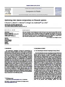
The inverse of T is sparse, which is an indication of a sparse state structure. A computational network that models multiplication by T is depicted in figure 1.1(a). The reader can readily verify that this network does indeed compute [y1 y2 y3 y4 ] = [u1 u2 u3 u4 ]T by trying the scheme on vectors of the form [1 0 0 0] up to [0 0 0 1]. The computations in the network are split into sections, which we will call stages, where the k-th stage consumes uk and produces yk . At each point k the processor in the stage active at that point takes its input data uk from the input sequence u and computes new

INTRODUCTION u1

u2

1

1 z

(a)

z

x2

x3

1

z

x4 1/12

z

1/6

1 1/4

z

1/3

z

1/2

u4

1/24

y1

y2

y3

y4

u1

u2

u3

u4

1

1/2 z

x2

1 1/3 1

(b)

u3

y1

1/3 z

x3

1 1/4 1

y2

3

1/4 z

1

x4 1

y3

y4

Figure 1.1. Computational networks corresponding to T . (a) Direct (trivial) realization, (b) minimal realization.

output data yk which is part of the output sequence y generated by the system. The dependence of yk on ui (i < k) introduces intermediate quantities xk which we have called states, and which subsume the past history of the system as needed in future calculations. This state xk is temporarily stored in registers indicated by the symbol z in the figure.1 The complexity of the computational network is highly dependent on the number of states at each point. A non-trivial computational network to compute y = uT which requires less states is shown in figure 1.1(b). The total number of (non trivial) multiplications in this network is 5, as compared to 6 in a direct computation using T. Although we have gained only one multiplication here, for a less moderate example, say an (n × n) upper triangular matrix with n = 10000 and d n states at each point, the number of multiplications in the network can be as low as 8dn, instead of roughly 1 2 2 n for a direct computation using T.

1 This

is a relic of an age-old tradition in signal processing which has little meaning in the present figure.

4


The (linear) computations in the network can be summarized by the following recursion, for k = 1 to n: xk+1 yk

⇔

y = uT

= =

xk A k + u k B k xkCk + uk Dk

or

[xk+1

yk ] = [xk

uk ] Tk ;

Tk =

Ak Bk

Ck Dk

(1.2)

in which xk is the state vector at time k (taken to have dk entries), Ak is a dk × dk+1 (possibly non-square) matrix, Bk is a 1 × dk+1 vector, Ck is a dk × 1 vector, and Dk is a scalar. More general computational networks may have any number of inputs and outputs, possibly also varying from stage to stage. In the example, we have a sequence of realization matrices

T1 =

·

· 1=2 1

;

T2 =

1=3 1 1=3 1

;

T3 =

1=4 1 1=4 1

;

T4 =

· 1 · 1

;

where the ‘·’ indicates entries that actually have dimension 0 (i.e. disappear) because the corresponding states do not exist. The recursion in equation (1.2) shows that it is a recursion for increasing values of k: the order of computations in the network is strictly from left to right, and we cannot compute yk unless we know xk , i.e., until we have processed u1 ; · · · ; uk−1 . Note that yk does not depend on uk+1 ; · · · ; un . This causality is a direct consequence of the fact that T has been chosen upper triangular, so that such an ordering of computations is indeed possible.

Time-varying systems We obtain an obvious link with system theory when we regard T as the input-output map, alias the transfer operator, of a non-stationary causal linear system with input u and output y = uT. The i-th row of T then corresponds to the impulse response of the system when excited by an impulse at time instant i, that is, the output y caused by an input u with uk = δi−k , where δk is the Kronecker delta. The case where T has a Toeplitz structure then corresponds to a time-invariant system for which the response to an impulse at time i + 1 is just the same as the response to an impulse at time i, shifted over one position. The computational network is called a state realization of T, and the number of states at each point in time is called the system order of the realization at that point. For time-invariant systems, the state realization can be chosen constant in time. For a time-varying system, the number of state variables need not be constant: it can increase and shrink. In this respect the time-varying realization theory is much richer, and we shall see in a later chapter that a time-varying number of states will enable the accuracy of some approximating computational network of T to be varied in time at will. If the network is regarded as the model of a physical time-varying system rather than a computational network, then the interpretation of a time-varying number of states is that the network contains switches that can switch on or off a certain part of the system and thus can make some states inaccessible for inputs or outputs at certain points in time.

INTRODUCTION

5

Sparse computational models If the number of state variables is relatively small, then the computation of the output sequence is efficient in comparison with a straight computation of y = uT. One example of an operator with a small number of states is the case where T is an upper triangular band matrix: Ti j = 0 for j − i > p. The state dimension is then equal to or smaller than p − 1, since only p − 1 of the previous input values have to be remembered at any point in the multiplication. However, the state model can be much more general, e.g., if a banded matrix has an inverse, then this inverse is not bounded but is known to have a sparse state realization (of the same complexity) too, as we had in the example above. Moreover, this inversion can be easily carried out by local computations on the realization of T:2 if T −1 = S, then u = yS can be computed via

xk+1 yk

= =


⇔

xk+1 uk

= =

−1 xk (Ak −Ck D−1 k Bk ) + yk Dk Bk −1 −1 −xkCk Dk + yk Dk

hence S has a computational model given by

Sk =

Ak −Ck D−1 k Bk D−1 B k k

−Ck D−1 k D−1 k

(1.3)

Observe that the model for S = T −1 is obtained in a local way from the model of T: Sk depends only on Tk . Sums and products of matrices with sparse state structures have again sparse state structures with number of states at each point not larger than the sum of the number of states of its component systems, and computational networks built with these compositions (but not necessarily minimal ones) can easily be derived from those of its components. In addition, a matrix T 0 that is not upper triangular can be split (or factored) into an upper triangular and a strictly lower triangular part, each of which can be separately modeled by a computational network. The computational model of the lower triangular part has a recursion that runs backward: x0k−1 yk

= =

x0k A0k + uk B0k x0kCk0 + uk D0k :

The model of the lower triangular part can be used to determine a model of a unitary upper matrix U which is such that U ∗ T is upper and has a sparse state structure. Thus, computational methods derived for upper matrices, such as the above inversion formula, can be generalized to matrices of mixed type [vdV95]. Besides matrix inversion, other matrix operations that can be computed efficiently using sparse computational models are for example the QR factorization (chapter 6) and the Cholesky factorization (chapter 13). At this point, the reader may wonder for which class of matrices T there exists a sparse computational network (or state realization) that realizes the same multiplication operator. A general criterion will be derived in chapter 5, along with a recursive 2 This

applies to finite matrices only, for which the inverse of the matrix is automatically upper triangular again and Dk is square and invertible for all k. For infinite matrices (operators) and block matrices with non-uniform dimensions, the requirement is that T must be outer. See chapters 6 and 7.

6


11 12 13 14 15

H2

22 23 24 25

T

H3

33 34 35

=

H4

44 45

..

.

55

Figure 1.2.

Hankel matrices are (mirrored) submatrices of T .

algorithm to determine such a network for a given matrix T. The criterion itself is not very complicated, but in order to specify it, we have to introduce an additional concept. For an upper triangular (n × n) matrix T, define matrices Hi (1 ≤ i ≤ n), (which are mirrored submatrices of T ), as 2

Ti−1;i

6 6 Ti−2;i Hi = 6 6 . 4 ..

Ti−1;i+1

3

···

Ti−1;n .. 7 . 7

Ti−2;i+1 ..

···

T1;i

. T1;n−1

7 7 T2;n 5

T1;n

(see figure 1.2). The Hi are called (time-varying) Hankel matrices, as they have a Hankel structure (constant along anti-diagonals) if T has a Toeplitz structure.3 In terms of the Hankel matrices, the criterion by which matrices with a sparse state structure can be detected is given by the following theorem, proven in chapter 5. Theorem 1.1 The number of states that are required at stage k in a minimal computational network of an upper triangular matrix T is equal to the rank of its k-th Hankel matrix Hk . Let’s verify this statement for our example matrix (1.1). The Hankel matrices are H1 = [ · · · · ] ;

H3 =

1=3 1=12 1=6 1=24

H2 = [1=2 1=6 1=24 ] ; 2

;

3

1=4 4 1 =12 5 : H4 = 1=24

3 Warning: in the current context (arbitrary upper triangular matrices) the H do not have a Hankel struci ture and the predicate ‘Hankel matrix’ could lead to misinterpretations. The motivation for the use of this terminology can be found in system theory, where the Hi are related to an abstract operator HT which is commonly called the Hankel operator. For time-invariant systems, HT reduces to an operator with a matrix representation that has indeed a traditional Hankel structure.

INTRODUCTION

7

Since rank(H1 ) = 0, no states x1 are necessary. One state is required for x2 and one for x4 , because rank(H2 ) = rank(H4 ) = 1. Finally, also only one state is required for x3 , because rank(H3 ) = 1. In fact, this is (for this example) the only non-trivial rank condition: if one of the entries in H3 would have been different, then two states would have been necessary. In general, rank(Hi ) ≤ min(i − 1; n − i + 1), and for a general upper triangular matrix T without state structure, a computational model indeed requires at most min(i − 1; n − i + 1) states for xi . The statement is also readily verified for matrices with a band structure: if the band width of the matrix is equal to d, then the rank of each Hankel matrix is at most equal to d. As we have seen previously, the inverse of such a band matrix (if it exists) has again a low state structure, i.e., the rank of the Hankel matrices of the inverse is again at most equal to d. For d = 1, such matrices have the form (after scaling of each row so that the main diagonal entries are equal to 1) 2

T

6 4

=6

1

−a1 1

3

−a2 1

7 7

; −a3 5 1

2 6

T −1 = 6 4

1

a1 1

a1 a2 a2 1

3

a1 a2 a3 a2 a3 7 7 a3 5 1

and it is seen that H3 of T −1 is indeed of rank 1.

1.2 OBJECTIVES OF COMPUTATIONAL MODELING Operations With the preceding section as background material, we are now in a position to identify in more detail some of the objectives of computational modeling, as covered by this book. Many of the basic operations will assume that the given operators or matrices are upper triangular. Applications which involve other types of matrices will often require a transformation which converts the problem to a composition of upper (or lower) triangular matrices. For example, a vector-matrix multiplication with a general matrix can be written as the sum of two terms: the multiplication of the vector by the lower triangular part of the matrix, and the multiplication by the upper-triangular part. Efficient realizations for each will yield an efficient overall realization. In the case of matrix inversion, we would rather factor the matrix into a product of a lower and an upper triangular matrix, and treat the factors independently. We will look at the class of matrices or operators for which the concept of a “sparse state structure” is meaningful, such that the typical matrix considered has a sequence of Hankel matrices that all have low rank (relative to the size of the matrix), or can be well approximated by a matrix that has that property.

Realization and cascade factorization.

A central question treated in this book is given a matrix (or operator), find a computational model {Tk }n1 of minimal complexity. Such a model could then e.g., be used to efficiently compute multiplications of vectors by T. Often we want additional properties to be fulfilled, in particular we wish the computations to be numerically stable. One important strategy is derived from classical filter theory. It starts out by assuming T to be contractive (i.e., kT k ≤ 1; if this is not the case, a normalization would pull the trick). Next, it subdivides the

8

TIME-VARYING SYSTEMS AND COMPUTATIONS Realization Transferoperator

T=

T

Factorization

Embedding State space realization A C B D

Lossless embedding

Lossless cascade realization

Σ

Approximation

Figure 1.3.

Objectives of computational modeling for matrix multiplication. u3 0

u4 0

u5 0

u2 0

u6 0

u1 0

u7 0 u8 0

y1

y2

∗

y3 y4

∗ y5

∗

∗

∗

∗

∗

∗

y6

y7

y8

Figure 1.4. Cascade realization of a contractive 8 × 8 matrix T , with a maximum of 3 states at each point. The number of algebraic operations is minimal.

question in four subproblems, connected schematically as in figure 1.3: (1) realization of T by a suitable computational model, (2) embedding of this realization into a larger model that consists entirely of unitary (lossless) stages, (3) factorization of the stages of the embedding into a cascade of elementary (degree-1) lossless sections in an algebraically minimal fashion. One can show that this gives an algebraically minimal scheme to compute multiplications by T. At the same time, it is numerically stable because all elementary operations are bounded and cannot magnify intermediate errors due to noise or quantizations. A possible minimal computational model for an example matrix T that corresponds to such a cascade realization is drawn in figure 1.4. In this figure, each circle indicates an elementary rotation of the form [a1

b1 ]

cos(θ) − sin(θ) sin(θ) cos(θ)

= [a2

b2 ] :

The precise form of the realization depends on whether the state dimension is constant, shrinks or grows. The realization can be divided into elementary sections, where each

INTRODUCTION

9

section describes how a single state entry of xk is mapped to an entry of the “next state” vector xk+1 . The cascade realization in figure 1.4 has a number of additional interesting properties. First, the number of operations to compute the next state and output is linear in the number of states at that point, rather than quadratic as would be the case for a general (non-factored) realization. Another is that the network is pipelinable, meaning that as soon as an operation has terminated it is ready to receive new data. This is interesting if the operation ‘multiplication by T’ is to be carried out on a collection of vectors u on a parallel computer or on a hardware implementation of the computational network. The property is a consequence of the fact that the signal flow in the network is strictly uni-directional: from top left to bottom right. Computations on a new vector u (a new uk and a new xk ) can commence in the top-left part of the network, while computations on the previous u are still being carried out in the bottom-right part.

Approximation.

It could very well be that the matrix that was originally given is known via a computational model of a very high order, e.g., via a series expansion. Then intermediate in the above sequence of steps is (4) the approximation of a given realization of T by one that has the lowest possible complexity given an acceptable tolerance. For example, it could happen that the given matrix T is not of low complexity because numerical inaccuracies of the entries of T have increased the rank of the Hankel matrices of T, since the rank of a matrix is a very sensitive (ill-conditioned) parameter. But even if the given matrix T is known to be exact, an approximation by a reducedorder model could be appropriate, for example for design purposes in engineering, to capture the essential behavior of the model. With such a reduced-complexity model, the designer can more easily detect that certain features are not desired and can possibly predict the effects of certain changes in the design; an overly detailed model would rather mask these features. While it is fairly well known in linear algebra how to obtain a (low-rank) approximant for certain norms to a matrix close to singular (e.g., by use of the singular value decomposition (SVD)), such approximations are not necessarily appropriate for our purposes, because the approximant should be upper triangular again and have a lower system order than before. Moreover, the original operator may be far from singular. Because the minimal system order at each point is given by the rank of the Hankel matrix at that point, a possible approximation scheme is to approximate each Hankel operator by one that is of lower rank (this could be done using the SVD). The approximation error could then very well be defined in terms of the individual Hankel matrix approximations as the supremum over these approximations. Because the Hankel matrices have many entries in common, it is not immediately clear whether such an approximation scheme is feasible: replacing one Hankel matrix by one of lower rank in a certain norm might make it impossible for the other Hankel matrices to find an optimal approximant such that the part that they have in common with the original Hankel matrix will coincide with the original approximation. In other words: each individual local optimization might prevent a global optimum. The severity of this dilemma is mitigated by a proper choice of the error criterion. It is truly remarkable that this dilemma has a neat solution, and that this solution can be obtained in a closed form. The error for

10


which a solution is obtained is measured in Hankel norm: it is the supremum over the spectral norm (the matrix 2-norm) of each individual Hankel matrix,

k T kH

=

sup k Hi k ; i

and a generalization of the Hankel norm for time-invariant systems. In terms of the Hankel norm, the following theorem holds true and generalizes the model reduction techniques based on the Adamjan-Arov-Krein paper [AAK71] to time-varying systems: Theorem 1.2 ([DvdV93]) Let T be a strictly upper triangular matrix and let Γ = diag(γi ) be a diagonal Hermitian matrix which parametrizes the acceptable approximation tolerance (γi > 0). Let Hk be the Hankel matrix of Γ−1 T at stage k, and suppose that, for each k, none of the singular values of Hk are equal to 1. Then there exists a strictly upper triangular matrix Ta whose system order at stage k is equal to the number of singular values of Hk that are larger than 1, such that

k Γ−1 (T − Ta) kH

≤ 1:

In fact, there is an algorithm that determines a state model for Ta directly from a model of T. Γ can be used to influence the local approximation error. For a uniform approximation, Γ = γ I, and hence kT − Ta kH ≤ γ : the approximant is γ-close to T in Hankel norm, which implies in particular that the approximation error in each row or column of T is less than γ. If one of the γi is made larger than γ, then the error at the i-th row of T can become larger also, which might result in an approximant Ta that has fewer states. Hence Γ can be chosen to yield an approximant that is accurate at certain points but less tight at others, and whose complexity is minimal. The realization problem is treated in chapter 5, the embedding problem is the subject of chapter 12, while the cascade factorization algorithm appears in chapter 14. The Hankel-norm approximation problem is solved in chapter 10.

QR factorization and matrix inversion.

Direct methods to invert large matrices may give undesired “unstable” results. For example, suppose we try to invert 2 6 6 6 6 T =6 6 6 4

..

.

3

..

. 1

0

−2 0 1 −2 1 −2 1

7 7 7 7 7 7 .. 7 . 5

..

.

INTRODUCTION

11

The inverse obtained by truncating the matrix to a large but finite size and inverting this part using standard linear algebra techniques produces 2 6 6 6 ? 6 T −1 = 6 6 6 4

..

.

.. . 1

0

.. . 2 4 8 1 2 4 1 2 1

3 7

··· 7 7 7 7 7 7 ··· 5

..

.

Clearly, this inverse is not bounded as we let the size of the submatrix grow. The true inverse is given by 2

..

. . .. 6 6 · · · −1=2 0 0 6 6 −1=4 −1=2 0 −1 T =6 6 −1=8 −1=4 −1=2 0 6 6 · · ·−1=16 −1=8 −1=4 −1=2 4 .. .. . .

3 7 7 7 7 7: 7 .. 7 .7 5

..

.

Note that it is lower triangular, whereas the original is upper triangular. How could this have happened? We can obtain valuable insights in the mechanics of this effect by representing the matrix as a linear system for which it is the transfer operator: T (z) = 1 − 2z

⇒

T −1 (z) =

1 1 − 2z

=

1 + 2z + 4z2 + · · · − 12 z−1 − 14 z−2 − · · · :

Among other things, this will allow us to handle the instability by translating “unstable” into “anti-causal” yet bounded. In the above case, we see that T −1 (z) has a pole inside the unit circle: it is not minimum phase and hence the causality reverses. With time-varying systems, much more is possible. In general, we can conceptually have a time-varying number of zeros inside and outside the unit circle, —conceptually, because the notion of poles and zeros is not very well defined for time-varying systems. We can also have zeros that move from inside the circle to outside, or the other way around. This means that the inversion of infinite matrices is much more difficult, but also more interesting, than in the finite case. The key to solving such inversion problems is to first compute a QR factorization, or “inner-outer factorization” in the system theoretical framework. This can be done using the realization of T as obtained earlier, hence can be done efficiently even on infinite-size matrices, and not surprisingly gives rise to time-varying Riccati equations. The inversion then reduces to inversion of each of the factors. We derive the time-varying equivalent of the above example in chapter 7. Other factorizations, such as the Cholesky factorization, are discussed in chapter 13.

Interpolation and matrix completion.

Several other topics are of interest as well. An important part of classical functional analysis and operator theory centers

12


around solving constrained interpolation problems: e.g., given “points” in the complex plane and “values” that a matrix-valued function should take in these points, construct an function that is constrained in norm and interpolates these values. In our present context, the functions are simply block-matrices or operators, the points are block diagonals, and the values are block diagonals as well. In chapter 9, we derive algebraic equivalents for very classical interpolation problems such as the NevanlinnaPick, Schur, Hermite-Fejer and Nudel’man problems. These problems are tightly connected to the optimal approximation problem discussed above. Lossless J-unitary matrices play a central role, and are discussed in chapter 8. In linear system theory, interpolation problems have found application in the solution of robust control problems, as well as the minimal sensitivity problem: design a feedback such that a given system becomes stable and the worst-case energy amplification of a certain input to a certain output is smaller than a given bound. We treat only a single example of this: the solution of the four-block problem (section 9.7). Finally, we consider the Nehari extension problem: for a given upper triangular matrix, try to find a lower-triangular extension such that the overall matrix has a norm bounded by a prescribed value (section 10.6). Again, the solution is governed by Jlossless matrices.

Operands In the preceding section, the types of operations (realization, embedding, factorization, approximation, interpolation) that are considered in this book were introduced. We introduce now the types of operands to which these operations are applied. In principle, we work with bounded linear operators on Hilbert spaces of (vector) sequences. From an engineering point of view, such operators can be regarded as infinite-size matrices. The entries in turn can be block matrices. In general, they could even be operators, but we do not consider that case. There is no need for the block entries to have the same size: the only requirement is that all entries on a row of the operator have an equal number of rows, and all entries on a column of the operator have an equal number of columns, to ensure that all vector-matrix products are well defined. Consequently, the upper triangular matrices can have an “appearance” that is not upper triangular. For example, consider 3 2 .. .. .. . . 7 6 . 6 ··· 2 222 ··· 7 7 6 T

6 6 6 6 6 ··· 4

=6

22 222 222 22 222 22 22 2 22 2 .. .

.. .

7 7 7 7 7 ··· 7 5

..

:

.

where in this case each box represents a complex number. The main diagonal is distinguished here by filled boxes. We say that such an operator describes the input-output behavior of a linear timevarying system. The system is time invariant if the matrix representation of the operator is (block) Toeplitz: constant along diagonals. In general, we allow the upper trian-

INTRODUCTION

13

gular part to have an arbitrary structure, or even no structure at all. Special cases are periodically varying systems, which give block-Toeplitz operators, and systems that are time-invariant outside a finite interval in time, which give operators that are constant at the borders. A sequence on which the operator can be applied (the input of the system) is represented by a row vector whose entries are again finite-size vectors conforming to the block entries of the operator. This corresponds to a system with block inputs and block outputs. If the size of the block entries is not constant, then the system has a time-varying number of inputs and outputs, which corresponds physically to a system with switches that are used to switch on or off certain inputs and outputs at certain times. It is possible to model finite matrices this way, as was shown in the introduction. For finite matrices, there are no inputs and outputs before and after a certain interval in time. A causal system corresponds to an operator whose matrix representation is upper triangular. We are interested in such systems because causality implies a computational direction: usually we can start calculations at the top-left end of the matrix and work towards the bottom-right end. Causality also introduces the notion of state. We allow the number of states to be time varying as well. This can be realized, for example, by switches that connect or disconnect parts of the system. The concept of a time-varying number of states allows the incorporation of a finer level of detail at certain intervals in time.

1.3 CONNECTIONS AND ALTERNATIVE APPROACHES Low displacement rank In recent times there has been quite an effort to study “structured matrices” in various guises. Besides sparse matrices (matrices with many zero entries) which fall within the context of our theory, two classical examples of structured matrices are the Toeplitz and Hankel matrices (matrices that are constant along diagonals or anti-diagonals). They represent the transfer operator of linear time-invariant (LTI) systems. The associated computational algorithms are well known. For example, for Toeplitz systems we have – Schur recursions for LU and Cholesky factorization [Sch17, Kai86], – Levinson recursions for the factorization of the inverse [Lev47], – Gohberg/Semencul recursions for computing the inverse [GS72], – Recursions for QR factorization [CKL87]. These algorithms have computational complexity of order O(n2 ) for matrices of size (n × n), as compared to O(n3 ) for algorithms that do not take the Toeplitz structure into account. Generalizations of the Toeplitz structure are obtained by considering matrices which have a displacement structure [KKM79, LK84, LK86, LK91]: matrices G for which there are (simple) matrices F1 , F2 such that G − F1∗GF2

(1.4)

is of low rank, α say. This type of matrices occurs, e.g., in stochastic adaptive prediction problems such as the covariance matrix of the received stochastic signal; the matrix

14


is called of low displacement rank or α-stationary. Toeplitz matrices are a special case for which F1 = F2 are shift matrices Z and α = 2. Related examples are block-Toeplitz and Toeplitz-block matrices, and, e.g., the inverse of a Toeplitz matrix, which is itself not Toeplitz yet has a displacement rank of α = 2. An overview of inversion and factorization algorithms for such matrices can be found in [Chu89]. Engineering applications are many, notably adaptive filtering [SK94]. In this book we do not consider low displacement matrices further (except sporadically in chapter 3, see section 3.6) and refer the reader to the extensive literature. Low displacement rank presupposes a structure that brings the operator under consideration “close to time-invariant”. If an operator has that property, then it is very important to recognize and utilize it since it leads to efficient algorithms for almost any operation related to the operator. In addition, matrix-vector multiplication and inversion of a system of equations can then be done using an adaptation of the fast Fourier transform (FFT). It is possible to combine the properties of low-displacement matrices with a time-varying system theoretic approach, an account can be found in [Dew97].

Stability and control The traditional focus of time-varying system theory has been control system design and related problems such as the stability of the system, optimal control, identification and modeling. On these topics there are quite a number of attractive textbooks and treatments, we mention [FS82, Kam79, Rug93]. Although some of the issues will appear in this book, they will not be our focus, which is essentially computational. We do give an extensive treatment of system identification—a central piece of theory—with the purpose of finding useful realizations for a linear operation. Reachability and observability spaces of a system will be omnipresent in many of our topics, such as in system approximation, algebraic operations on systems, embedding, and parametrization. The theory that we develop parallels the classical identification theory for time-varying systems, possibly in a more concrete way. The notion of “uniform exponential stability” plays a central role in our theory as well. A linear computational scheme will have to be stable or it will not be usable. Many theorems are only valid under the condition of stability. However, conditions on stability of a system is not a great point of interest in the book, and we shall mostly assume them as a matter of course. While this book was under redaction, Halanay and Ionescu published a book on linear time-varying discrete systems [HI94], using a framework very much like ours (and in fact partly inspired by it via publications in the mathematical literature). The contents of that book is very relevant to the work presented here, although the type of problems and their approach is often quite different. In the book of Halanay and Ionescu, basic concepts such as external factorization, inner-outer factorization, and J-inner embedding are related to the solution of specific types of (time varying) Riccati equations. We provide the derivation of the relevant Riccati equations as well, but systematically put them into a geometric context—the context provided by the reachability and observability operators of the system under consideration. On a number of other issues, the two books are unrelated. Halanay and Ionescu give an extensive treatment of optimal control and the related game theory. Although we treat some as-

INTRODUCTION

15

pects of the former, e.g., the four block problem, we do not consider the latter topic. On the other hand, since our focus is computational, we provide attractive algorithms such as “square root algorithms”, parametrizations, and give an extensive treatment on model reduction and approximation. We have aimed at a textbook which could be used by engineering students with a good knowledge of linear algebra, but only a rudimentary knowledge of Hilbert space theory. We thought it remarkable that most essential properties could be approached from a relatively elementary point of view based on the geometry of reachability and observability spaces.

On the origin of this work The ansatz for the computational modeling as studied in this book was a generalization of the Schur interpolation method to provide approximations of matrices to matrices with banded inverses, by Dewilde and Deprettere [DD87, DD88]. The motivation driving this research was the need to invert large matrices that occur in the finite element modeling of VLSI circuits [JD89, Nel89]. Subsequent research by Alpay, Dewilde, and Dym introduced an elegant diagonal notation by which the Schur interpolation method and similar such generalized, time-varying interpolation problems could be described [ADD90]. In these days, it became clear that the solution of many (time-invariant) interpolation problems can effectively be formulated in state space terms [BGR90]. The new diagonal notation was thus adopted and applied to the description of time-varying state space systems, resulting in a realization theory [vdVD91], orthogonal embedding theory with application to structural factorization [vdVD94a, vdVD93], and later an optimal Hankel-norm model reduction theory as well [DvdV93], and culminated in a workshop on the topic [DKV92], and the thesis of Van der Veen [vdV93b]. Subsequent work was on widening the algebraic aspects of the new theory [vdV96, GvdV96, vdV95], as well as H∞ control aspects [Yu96, SV95, YSvdVD96, SV96]. The above provides the background for this book. In the mean time, there are many connections to parallel work by the “Amsterdam group” (Kaashoek, Gohberg, and coworkers) to interpolation and operator extension [GKW89, Woe89, GKW91, BGK92a], and to realization of time-varying systems [GKL92, BAGK94].

I

REALIZATION

2

NOTATION AND PROPERTIES OF NON-UNIFORM SPACES

Time-varying linear systems can be compactly described by a recently developed notation in which the most important objects under consideration, sequences of vectors and the basic operators on them, are represented by simple symbols. Traditional timevarying system theory requires a clutter of indices to describe the precise interaction between signals and systems. The new notation helps to keep the number of indices in formulas at a minimum. Since in our case sequences of vectors may be of infinite length, we have to put them in a setting that can handle vectors of infinite dimensions. “Energy” also plays an important role, and since energy is measured by quadratic norms, we are naturally led to a Hilbert space setting, namely to Hilbert spaces of sequences of the `2 -type. This should not be too big a step for engineers versed in finite vector space theory since most notions of Euclidean vector space theory carry over to Hilbert spaces. Additional care has to be exercised, however, with convergence of series and with properties of operators. The benefit of the approach is that matrix theory and system theory mesh in a natural way. To achieve that we must introduce a special additional flavor, namely that the dimensions of the entries of the vectors considered are not necessarily all equal. The material covered in this chapter provides a minimal “working basis” for subsequent chapters. Additional properties and more advanced operator theoretic results are covered in chapter 4. A brief review of Hilbert space definitions and results which are relevant to later chapters can be found in Appendix A. In this work, we only need the space `2 of bounded sequences, subspaces thereof, and bounded operators on these spaces. 19

20


2.1 SPACES OF NON-UNIFORM DIMENSIONS Non-uniform sequences Let us consider (possibly infinite) sequences whose entries ui are finite dimensional vectors: u = [ · · · u−1 u0 u1 u2 · · · ] : (2.1) Typically, we write such sequences out as rows of (row) vectors. We say that u represents a signal, where each component ui is the value of the signal at time instant i. The square surrounding u0 identifies it as the entry with index zero. If the ui are scalar, then u is a one-channel signal. A more general situation is obtained by taking the ui to be (row) vectors themselves, which makes u a multi-channel signal. It is not necessary that all ui have equal dimensions: we allow for a time-varying number of channels, or equivalently, for non-uniform sequences. (Physically, such signals could be obtained by switches.) In order to specify such objects more precisely, we introduce the notion of index sequences. Let {Ni ∈ N ; i ∈ Z}be an indexed collection of natural numbers1, such that ui ∈ C Ni : Ni is the dimension of the vector ui . The sequence N, N = [ Ni ]∞ −∞

= [···

N−1

N0

N1

N2

· · · ] ∈ NZ

is called the index sequence of u. (The symbol N Z indicates the set (Cartesian product) of copies of N indexed by elements of Z.) If we define Ni = C Ni , then signals (2.1) live in the space of non-uniform sequences which is the Cartesian product of the Ni :

N = · · · × N−1 × N0 × N1 × N2 × · · · =: C N Conversely, if N

= CN,

;

then to retrieve the index sequence N from N we write N

=

#(N ) :

A signal in N can be viewed as an infinite sequence that has a partitioning into finite dimensional components. Some of these components may have zero dimension (Ni = 0) to reflect the fact that no input signal is present at that point in time. In that case, we write ui = · , where ‘ · ’ is a marker or placeholder. Mathematically, ‘ · ’ can be viewed as the neutral (and only) element of the Hilbert space C 0 , the vector space of dimension zero. Formally, we must define some calculation rules with sequences or matrices that have blocks with dimension zero. Aside from obvious rules, the product of an “empty” matrix of dimension m × 0 and an empty matrix of dimension 0 × n is a matrix of dimension m × n with all elements equal to 0. All further rules of block matrix multiplication remain consistent. Using zero dimension indices, finite dimensional vectors are incorporated in the space of non-uniform sequences, by putting Ni = 0 for i outside a finite interval. We usually do not write these trailing markers if their presence is clear from the context or otherwise not relevant: this is consistent with the fact that for any set A, 1 Z denotes

the set of integers, N the non-negative integers {0; 1; · · ·}, and C the complex numbers.


21

A × C 0 = A. With abuse of notation, we will also usually identify C 0 with the empty set ;. We say that a signal u as in (2.1) has finite energy if the sum ∞

∑ k ui k22

i=−∞

is finite. In that case we say that u belongs to `N 2 , the space of (non-uniform) sequences in N with finite `2 norm. `N is a ’Hilbert space’, it is even a separable Hilbert space, 2 which means that it has a countable basis. A Hilbert space of non-uniform sequences is of course isomorphic to a standard `2 Hilbert space, the non-uniformity provides an additional structure which has only system theoretical implications. The inner product of two congruent (non-uniform) sequences f ; g in N is defined in terms of the usual inner product of (row)-vectors in Ni as (

f ; g)

=

∑ ( fi

;

gi )

i

where ( fi ; gi ) = fi g∗i is equal to 0 if Ni is defined by u = [ ui ]∞ −∞ :

=

0, by definition.2 The corresponding norm

k u k22 = (u

∞

;

u)

=

∑ k ui k22

i=−∞

so that k u k22 represents the energy of the signal. `N 2 can thus be viewed as an ordinary separable Hilbert space of sequences on which a certain regrouping (of scalars into finite dimensional vectors) has been superimposed. Consequently, properties of Hilbert spaces carry over to the present context when this grouping is suppressed. To illustrate some of the above, let N = [ · · · 0 0 1 3 2 0 0 · · · ]. The vector u = [ 6 ; [3 2 1] ; [4 2] ] is an element of the non-uniform sequence space N = C N , suppressing entries with zero dimensions. The norm of u is given by k u k2 = [62 + (32 + 22 + 12 ) + (42 + 22 )]1=2 . We see that classical Euclidean vector space theory fits in easily.

Operators on non-uniform spaces

Let M and N be spaces of sequences corresponding to index sequences M, N. When we consider sequences in these spaces as signals, then a system that maps ingoing signals in M to outgoing signals in N is described by an operator from M to N : T : M → N;

y = uT :

Following [ADD90, DD92], we adopt a convention of writing operators at the right of input sequences: y = uT. If for some reason there is confusion, we use brackets: 2∗

denotes the complex conjugate transpose of vectors or matrices, or the adjoint of operators.

22


‘T (u)’. This unconventional notation is perhaps unnatural at first, but it does have advantages: signals correspond to row sequences, circuit diagrams read like the formulas, and the inverse scattering problem, which we shall treat extensively, appears more natural. Continuous applications of maps such as “STU · · ·” associate from left to right (uSTU := ((uS)T )U) and can often be interpreted as matrix products. Things get more complicated when S or T are maps defined on more complex objects than sequences. Notable examples are projection operators defined on spaces of operators, and the socalled Hankel operator which is introduced in the next chapter. N We denote by X (M; N ) the space of bounded linear operators `M 2 → `2 : an operM ator T is in X (M; N ) if and only if for each u ∈ `2 , the result y = uT is in `N 2 , and so that k T k = sup kkuTu kk2 2 u∈` ;u6=0 M

2

is bounded. k T k is called the induced operator norm of T. A bounded operator defined everywhere on separable Hilbert spaces admits a matrix representation which uniquely determines the operator [AG81]: 2

..

6 6 6 6 ··· T = [Ti j ]∞ = i; j =−∞ 6 6 4

..

.. .

.

.

T−1;−1 T0;−1 T1;−1

T−1;0 T00 T10 .. .

..

T−1;1 T01 T11

.

3

7 7 7 ··· 7 7 7 5

..

(2.2)

.

(where the square identifies the 00-entry), so that it fits the usual vector-matrix multiplication rules. The block entry Ti j is an Mi × N j matrix. To identify the block-entries, rows and columns of T, it is convenient to have specific operators which construct a sequence from its entries. Following [ADD90], we define for a given space sequence N , the operator πk as · πk :

Nk → N :

aπk = a[ · · · 0 INk

0 ··· ]:

(2.3)

Thus, πk constructs a sequence out of an element of Nk , by embedding it into a sequence which is otherwise zero (or empty, depending on the context). We define an “adjoint” to πk as · π∗k : N → Nk : uk = uπ∗k : Thus, π∗k retrieves the k-th (block) entry of a sequence.3 We often implicitly use the facts that πk π∗k = INk and ∑k π∗k πk = IN , which is a “resolution of the identity”. Clearly, both πk and π∗k have matrix representations. If an operator T with a congruent matrix representation is positioned to the right of πk , then the (matrix or operator) product πk T makes sense and corresponds to taking the k-th row out of T. Similarly, Tπ∗k selects its k-th column. 3 Properly

speaking, the definition of an adjoint necessitates a Hilbert space context, but the operators do make obvious sense in a larger context as well.


23

The block entry Ti j of T is given by Ti j = πi Tπ∗j . With regard to (2.2), the operator Ti = πi T can be called the i-th (block) row of T, while Tπ∗j is the j-th column of T. In X (M; N ), we define the space of bounded upper operators

U (M N ) = {T ∈ X (M N ) : Ti j = 0 ;

;

(i > j )} ;

the space of bounded lower operators

L(M N ) = {T ∈ X (M N ) : Ti j = 0 ;

;

(i < j )} ;

and the space of bounded diagonal operators

D = U ∩L

:

As a matter of notational convenience, we often just write X ; U ; L; D when the underlying spaces are clear from the context or are of no particular relevance. For A ∈ D, “Ai ” serves as shorthand for the entry Aii , and we write A = diag[ · · · A−1

A1 · · · ] = diag[ Ai ] :

A0

U , L and D satisfy the following elementary properties [ADD90]: U ·U ⊂ U L∗ = U L·L ⊂ L U∗ = L D·D ⊂ D

(2.4)

:

A link with classical linear time invariant (LTI) is established easily. In the timeinvariant context, the sequences M and N are uniform, and the transfer operator behaves identically at each point in time: a shift of the input sequence over a few time slots produces still the same output sequence, but translated over the same shift. This translates to T having a Toeplitz structure: for all integers i, j and k, Ti; j = Ti+k; j+k , or, equivalently, all block entries on the same diagonal are equal. Toeplitz operators are often represented by their z-transform, which we define as follows. Denote by Tk the entry on the k-th diagonal (i.e., Tk = Ti;i+k for any i), and let +∞

T (z) =

∑

i=−∞

Tk zk ;

then T (z) is called the matrix-valued transfer function associated to T. Note that this definition is purely formal, there is no guarantee that the series converges at any point of the complex plane. Occasionally, we will use a “meta-operator” T which associates a Toeplitz representation to a transfer function: 2

T

..

.

6 6 .. 6 . 6 6 . (T (z)) = 6 . . 6 6 . 6 .. 4

..

.

..

.

..

.

..

.

..

.

..

T−1

T0

T1

T2

T3

T−2

T−1

T0

T1

T2

T−3 .. .

T−2 .. .

T−1 .. .

T0 .. .

T1 .. .

.

..

3

.

7

.. 7 . 7 7 .. 7: . 7 7 .. 7 . 7 5 .. .

24


Harmonic analysis on LTI systems will often provide interesting examples and counterexamples. If D ∈ D and invertible, then D−1 ∈ D, and (D−1 )i = (Di )−1 [ADD90]. However, unlike the situation for finite-size matrices on uniform sequences, the spaces U and L are not closed under inversion: if an upper operator T ∈ U is boundedly invertible, then the inverse is not necessarily upper. A simple example of this is given by the pair of Toeplitz operators 2 6 6 6 6 T =6 6 6 4

..

.

. 1

2

3

..

−2 1 −2

0

1

7 0 77 7 7; .. 7 .7 5

..

T

−1

.

3

..

. 6 6. 6 .. 6

0

0 −1=2 0 0 −1=4 −1=2 −1=8 −1=4 −1=2 .. .

6 =6 6 6 6· · · 4

7 7 7 7 7 7: 7 7 7 5

0 .. .

..

.

But also for finite-size matrices based on non-uniform space sequences, the same can happen. For example, let T : C 2 × C 1 → C × C × C , C n 2 1 2 4 1=2 T= C C 0

C

C

0 2

0 0 5; 1

1=4

C2

2

3

1 C T −1 = C 4 -1/4 C 1/16

C

0 1/2 -1/8

3

0 05 1

(2.5)

(the underscore identifies the position of the 0-th diagonal). When viewed as matrices without considering their structure, T −1 is of course just the matrix inverse of T. Mixed cases where the inverse has a lower and an upper part can also occur, and these inverses are not trivially computed, as they require a “dichotomy”: a splitting of spaces into a part that determines the upper part and a part that gives the lower part. The topic will be investigated in chapter 7. An important special case of upper operators with upper inverses is the following. An operator of the form (I − X ), where X is a bounded operator, has an inverse that is given by the series expansion (Neumann expansion) (I − X )

−1

2 = I + X + X + ···

(2.6)

when the series converges in norm. It is known in operator theory that this will be the case when the geometric series 1 + k X k + k X 2 k + · · · converges, which occurs when the spectral radius r(X ) of X is smaller than 1:4 r(X ) := lim

n→∞

k X n k1 n =

1) systems replaces the notion in LTI systems theory of poles (eigenvalues of A) that lie in, on, or outside the unit circle. For the general case we can state the following definition (cf. equation (3.7)). Definition 3.4 A 2 × 2 matrix of block diagonals T is said to be a realization of a transfer operator T ∈ U if the diagonals T[k] = P0 (Z−k T ) of T equal the diagonal expansion (3.7): 8 k < 0; < 0; D; k = 0; T[k] = (3.8) : (k) {k−1} B A C; k > 0: Equivalently, the entries Ti j of T are given by 8 < 0;

Ti j

=

Di ; : Bi Ai+1 · · · A j−1C j ;

i> j i= j i < j;

(3.9)

and it follows that the transfer operator which corresponds to the realization {A; B; C; D} has the matrix representation 2

6 6 6 6 6 T =6 6 6 6 4

..

.

.. . D−1

0

.. . B−1C0 D0

B−1 A0C1 B0C1 D1

B−1 A0 A1C2 B0 A1C2 B1C2 D2

3 7

··· 7 7

7 7 7: 7 7 ··· 7 5

..

.

(3.10)

40


Definition 3.5 Let T ∈ U . An operator T ∈ U is said to be locally finite if it has a state realization whose state space sequence B is such that each Bk has finite dimension. The order of the realization is the index sequence #(B) of B. The concept of locally finite operators is a generalization of rational transfer functions to the context of time-varying systems.

Realizations on X2

We can extend the realization (3.4) further by considering generalized inputs U in X2M and outputs Y in X2N : XZ−1 Y

=

XA + UB XC + UD :

=

(3.11)

If À < 1, then X = UBZ(I − AZ)−1 , so that X ∈ X2B . The classical realization (3.4) may be recovered by selecting corresponding rows in U, Y and X. Indeed, we can interpret the rows of U ∈ X2M as a collection of input sequences u ∈ `2M , applied simultaneous N to the system. Likewise, Y ∈ `N 2 contains the corresponding output sequences y ∈ `2 . This interpretation will be pursued at length in the following chapters. A recursive description for the realization (3.11) is a generalization of (3.1), and is obtained by selecting the k-th diagonal of U ; Y, and X in (3.11): (−1)

X[k+1] Y[k]

= =

X[k] A + U[k]B X[k]C + U[k] D :

(3.12)

(−1)

Note that the k-th diagonal of XZ−1 is X[k+1] , which contains a diagonal shift. The same remarks on the relation between this recursive realization and the equations (3.11) as made earlier on the `2 -realizations are in order here. Starting with chapter 5, we will heavily use this type of realizations, where we act on sequences of diagonals rather than scalars.

State transformations

Two realizations {A; B; C; D} and {A0 ; B0 ; C0 ; D0 } are called equivalent if they realize the same transfer operator T, D B(k) A{k−1}C

= =

D0 B0(k) A0{k−1}C0

(all

k ≥ 0) :

(3.13)

Given a realization of an operator T ∈ U , it is straightforward to generate other realizations that are equivalent to it. For a boundedly invertible diagonal operator R (sometimes called a Lyapunov transformation), inserting x = x0 R in the state equations (3.11)

TIME-VARYING STATE SPACE REALIZATIONS

leads to

⇔

⇔

⇔

x0 RZ−1 y

x0 R A x0 RC

= =

+

uB uD

+

x0 Z−1 R(−1) y

=

x0 Z−1 y

=

x0 RAR−(−1) + u BR−(−1) x0 RC + u D

x0 Z−1 y

=

=

=

x0 R A x0 RC

=

x0 A 0 x0C0

+ +

41

+ +

uB uD

uB0 uD0 :

Proposition 3.6 Let R ∈ D(B; B) be boundedly invertible in D. If {A; B; C; D} is a realization of a system with transfer operator T , then an equivalent realization is given by {A0 ; B0 ; C0 ; D0 }, where3

A0 B0

C0 D0

=

R I

A C B D

" h

R(−1)

In addition, the spectral radii of AZ and A0 Z are the same:

#

i−1

:

(3.14)

I À

= À 0 .

P ROOF We have already D = D0 , and B0(k) A0{k−1}C0 = B(k) R−(k−1) · R(k−1) A{k−1} R−(k−2) · R(k−2) A{k−2} R−(k−3) · · · R(1) A(1) R−1 · RC = B(k) A{k−1}C :

Stability is preserved under the transformation: `

RAR−(−1)

= = =

≤

limn→∞ k (RAR−(−1)Z)n k1=n limn→∞ k (RAZR−1 )n k1=n limn→∞ k R(AZ)n R−1 k1=n limn→∞ k R k1=n · k (AZ)n k1=n · k R−1 k1=n

(3.15) =

À

since k R k1=n → 1 and k R−1 k1=n → 1. Because À ≤ `RAR−(−1) can be proven in the same way, it follows that À = `RAR−(−1) . 2

If the realizations {A; B; C; D} and {A0 ; B0 ; C0 ; D0 } are related by (3.14) using bounded R with bounded R−1 , then we call them Lyapunov equivalent.

3.2 SPECIAL CLASSES OF TIME-VARYING SYSTEMS In this section, we examine the behavior of certain interesting subclasses of systems. Since it takes an infinite amount of data and time to describe a general time-varying 3 In

future equations, we write, for shorthand, R−(−1) := [R(−1) ]−1 .

42


system, it pays to consider special classes of operators in which computations can be carried out in finite time. Interesting classes are (1) finite matrices, (2) periodically varying systems, (3) systems which are initially time-invariant or periodic, then start to change, and become again time-invariant or periodic after some finite period (timeinvariant or periodic at the borders), (4) systems that are quasi-periodic with a given law of quasi-periodicity, and (5) systems with low displacement rank [KKM79]. Sometimes we can even treat the general case with finite computations, especially when we are interested only in the behavior of the system in a finite window of time.

Finite matrices Matrices of finite size can be embedded in the general framework in several ways. For example, if the input space sequence M = · · · ⊕ M−1 ⊕ M0 ⊕ M1 ⊕ · · · has Mi = ; for i outside a finite interval, [1; n] say, and if the output space sequence N has Ni = ; also for i outside [1; n], then T ∈ U (M; N ) is an upper triangular n × n (block) matrix: 2

· · 6 · 6

6 6 6 6 T =6 6 6 6 6 4

· · T11

· · T12 T22

··· ··· .. .

· · T1n T2n .. .

· · · ·

Tnn

· ·

· · · · .. .

3

7 7 2 7 T11 7 7 6 7 6 7≡6 7 4 7 · 7 7 · 5

T12 T22

··· ··· .. .

T1n T2n .. .

3 7 7 7 5

Tnn

· where “·” stands for an entry in which one or both dimensions are zero. We can choose the sequence of state spaces B to have zero dimensions outside the index interval [2; n] in this case, so that computations start and end with zero dimensional state vectors. Doing so yields computational networks in the form described in chapter 1. The finite matrices form an important subclass of the bounded operators, because (i) initial conditions are known precisely (a vanishing state vector) (ii) computations are finite, so that boundedness and convergence are not an issue (these issues become important again, of course, for very large matrices). In particular, À = 0 always. By taking the dimensions of the non-empty Mi non-uniform, block-matrices are special cases of finite matrices, and sometimes, matrices that are not upper triangular in the ordinary sense, are block-upper, i.e., in U (M; N ), where M and N are chosen appropriately. An example is given in figure 3.2(a). An extreme representative of a block-upper matrix is obtained by taking

M N

= =

··· ⊕ ··· ⊕

so that a matrix T ∈ U has the form 2

; ;

⊕ ⊕

· · · 6 · T12 6 T =4 ·

M1 ;

⊕ ⊕ 3

; N2

· · 7 7 ≡ [T12 ] ; · 5 ·

⊕ ⊕

;··· ;···


43

u1

z z z x2

(a)

(b)

y2

Figure 3.2. (a) A block-upper matrix; (b) a state realization of a special case of a blockupper matrix, T = [T12 ]. that is, T = T12 is just any matrix of any size. Figure 3.2(b) depicts the time-varying state realization of such a system. Inputs are only present at time 1, and outputs are only generated at time 2. The number of states that are needed in going from time 1 to time 2 is, for a minimal realization, equal to the rank of T12 , as we will see in the next section. There are applications in low-rank matrix approximation theory that use this degenerate view of a matrix [vdV96].

Time-invariant on the borders A second important subclass of time-varying systems are systems for which the state realization matrices {Ak ; Bk ; Ck ; Dk } are time-invariant for k outside a finite time interval, again say [1; n]. This class properly contains the finite matrix case. The structure resulting from such realizations is depicted in figure 3.3. Computations on such systems can typically be split in a time-invariant part, for which methods of classical system theory can be used, and a time-varying part, which will typically involve recursions starting from initial values provided by the time-invariant part. Boundedness often reduces to a time-invariant issue. For example, À is equal to max(r(A0 ); r(An+1 )), solely governed by the stability of the time-invariant parts.

Periodic systems A third subclass is the class of periodically varying systems. If a system has a period n, then it can be viewed as a time-invariant system T with block entries Ti j = Ti− j of size n × n: T is a block Toeplitz operator. The realization matrices {A; B; C; D} of this


44

Figure 3.3. Transfer operator of a system that is time-invariant on the borders. Only the shaded areas are non-Toeplitz. block operator are given in terms of the time-varying {Ak ; Bk ; Ck ; Dk } as A B

=

=

2A1 A2 · · · An ;

3

B1 A2 A3 · · ·An 6 B2 A3 · · ·An 7 6 7 6 .. 7 4 . 5

C D

= [ C1

2 6 6 4

= 6

Bn

D1

A1C2 A1 A2C3 · · · B1C2 B1 A2C3 · · · D2 B2C3 .. .

A1 · · · An−1Cn ] 3 B1 A2 · · · An−1Cn B2 A3 · · · An−1Cn 7 7 7 .. 5 . Dn

Computations involving such operators can often be done by taking it as a block timeinvariant system, which will provide exact initial conditions at the beginning of each period. These time-invariant solutions can be computed in classical ways. However, if the period is large, this may not be attractive, in which case the general methods may be more appealing. The classical Floquet theorem for time continuous systems which states that there is a periodic state transformation which transforms a periodic state transition matrix A(t ) into a time invariant one does not have a simple time discrete counterpart. A generic counterexample is a system with period 2 and A matrices given by 0 1 1 0 A2 = ; ; A1 = 0 0 0 1 and suppose that there would exist state transformation matrices R1 and R2 such that 01 −1 −1 2 R1 A1 R−1 2 = R2 A2 R1 =: α, then we should have (R1 αR1 ) = [ 0 0 ] which is impossible since this latter matrix has no square root.

Systems of low displacement rank An important class of structured matrices is formed by matrices of low “displacement rank”, and was extensively studied by Kailath and his many students and co-workers


45

[KKM79, KS95] (see in particular the theses of Lev-Ari [Lev83] and Sayed [Say92]). Although the brunch of this book is devoted to another kind of structure, namely lowdimensional state realizations, we give here a short introduction to low displacement matrices, and at the end of this chapter, we give a theory which combines results of the two theories, namely low complexity parametrizations for systems that are at the same time of low displacement type and of low systems rank. Let R be an n × n positive definite matrix, and let us define the n × n “displacement matrix”, alias restricted shift operator 2

0

0

6 6 1

..

.

4

..

.

σ=6 6

0

..

. 1

3 7 7 7: 7 5

0

This matrix is similar to the reverse shift operator Z∗ , but unlike Z∗ , it truncates the shifted sequence and introduces a zero, so that it is not an invertible operator. The displacement of R is defined as R−σRσ∗ [KKM79]. We assume that it has inertia ( p; o; q), which means that there exist matrices

G = [g0

g1 · · · gn−1 ] ;

J=

Ip

−Iq

of dimensions ( p + q) × n and ( p + q) × ( p + q) respectively, such that 2

R − σRσ∗

=

G∗ JG

6 6 4

= 6

3

g∗0 g∗1 .. .

7 7 7 J [g0 · · · gn−1 ] ; 5

g∗n−1 in which G has full row rank. It is convenient to split each entry gk according to the inertia formula: gk =

p q

gk1 gk2

:

α := p + q is called the displacement rank. If α is small compared to n, then R is said to be of low displacement rank. Clearly, R is parametrized by the entries of G. Important calculations on R such as the determination of its Cholesky factorization R = L∗ L or that of its inverse can be done efficiently on G rather than on R itself. In fact, this is not limited to positive definite matrices R, but can be generalized to any matrix T with (block matrix) entries. In the sequel we shall just look at additive and multiplicative decompositions of a positive definite matrix R = L∗ L = 12 (F + F ∗ ), because that covers the most important applications. The two notions, low displacement rank and low system order are not related to each other. We know of systems that score high for one and low for the other. The prototype example of a low displacement rank matrix is a Toeplitz matrix, which has displacement rank one or two. Such a matrix may not have a useful low dimensional state

46


space realization. For example, the LTI transfer function T (z) = z + 12 z2 + 13 z3 + · · · is of course of low displacement rank but no finite dimensional state space realization is capable of reproducing the decay 1n , characteristic of a transfer function of logarithmic type.

Uniformly exponentially stable systems Finally, a large class of systems for which precise and finite calculations are possible is the class of u.e. stable systems: systems that have a realization for which À < 1. Recursions on such systems are typically convergent, that is, independent of the precise initial value at point k as k → −∞. This means that it is possible to limit attention to a finite time-interval, and to obtain arbitrarily accurate initial values for this interval by performing a finite recursion on data outside the interval, starting with initial values set to 0. For example, if in a computation for k > 1, an initial state x1 is required, then this latter value can be approximated to arbitrary precision using a finite sequence of past input samples and system matrices, since 2

x1

=

x−n A−n · · · A0

+ [u−n

6 6 4

u−n+1 · · · u0 ] 6

B−n A−n+1 A−n+2 · · ·A0 B−n+1 A−n+2 · · ·A0 .. .

3 7 7 7: 5

(3.16)

B0 If the system is u.e. stable, then kA−n · · · A0 k can be made arbitrarily small by choosing n large enough. Neglect of the first term in (3.16) then gives an accurate approximation for x1 . The same approximation would of course be obtained by choosing x−n = 0 if that were possible, and computing x1 via the state recursion.

3.3 EXAMPLES AND EXTENSIONS

Using the connection of a matrix or operator in U and its realization as visualized in equation (3.10), we study some simple classes of matrices and their corresponding realizations, as well as some simple operations on matrices such as sums and products, a special case of matrix inversion, and extensions to more general realization frameworks.

Banded matrices One of the easiest examples of a matrix for which it is possible to write down a realization directly is the case of a banded matrix. Thus let T ∈ U be given by 2 6 6 6 T =6 6 4

T11

0

T12 T22

T1;d T2;d .. .

0 T2;d +1 .. . Tn−1;n−1

0 0

3

7 7 7 : Tn−d +1;n 7 7 5 Tn−1;n

Tn;n


47

The width of the band is in this case equal to d. A trivial realization for T requires up to d − 1 states per stage: 2

"

T1 =

·

·

6 6 6 6 Tk =6 6 6 4

#

1 T11

0 1

2

T2 =

1 0 T12

6 6 6 6 Tn−1 =6 6 6 4

#

0 1 T22

.

0

..

.

..

. 1 0

···

0 1

0 1

..

.

0

..

.

..

···

. 1 0

0 1

2

3

1 0 0 T13 6 7 T3 =4 0 1 0 T23 5 0 0 1 T33

Tn

3

7 7 7 7 7 7 Tk−1;k 7 5

Tk−d +2;k .. . Tk;k

Tn−d ;n−1

0 0

2

..

0 0

"

Tk−d +1;k

3

7 7 7 7 7 7 Tn−2;n−1 7 5

Tn−d +1;n−1 .. . Tn−1;n−1

3

· Tn−d +1;n 6 .. 7 6 · . 7

=6 6

4 ·

·

7

: Tn−1;n 7 5

Tn;n

This is not necessarily a minimal realization: there might exist realizations with a smaller number of states, depending on the precise values of Ti j . Even for general banded matrices, the number of states in the last d stages can be made smaller than presented here, although this will introduce some irregularities in the structure of these sections. Other matrices for which one can obtain realizations directly are matrices with a staircase band structure, and band matrices with some spurious entries in the upper right hand corner. The latter type of matrix arises in finite difference modeling of one dimensional differential equations with periodic boundary conditions (figure 3.4). In simple cases, the non-zero entries of the matrix are just +1 and −1 (for a first-order differential equation), and the matrix has a Toeplitz structure (constant along the diagonals). A three-diagonal matrix occurs with simple discretizations of second-order ODEs. Nonuniform spacing of the discretization points leads to banded matrices without the Toeplitz structure.

Sum of two realizations

Let T1 ; T2 ∈ U (M; N ) be two transfer operators, with realizations {A1 ; B1 ; C1 ; D1 } and {A2 ; B2 ; C2 ; D2 }, respectively. Then the sum of these two operators, T = T1 + T2 , has a realization given directly in terms of these two realizations as "

A

C

B D

2

# =

A1 6 0 4

0 A2

C1 C2

B1

B2

D1 + D2

3 7 5


48

0

0

Figure 3.4. A block-upper matrix with a maximal state dimension of 2. The main diagonal

is shaded; N1 = ; and Mn+1 = ;. This type of matrix arises after discretization in certain 1-D nite dierence modeling problems with periodic boundary conditions. The state dimension sequence of this realization is equal to the sum of the state dimension sequences of T1 and T2 . Note, however, that this realization is not necessarily minimal: there might exist a realization of T whose state dimension sequence is smaller (for reduction of the state space to minimal dimensions, see the next section).

Product of two realizations

The product of T1 ∈ U (M; N1 ) and T2 ∈ U (N1 ; N2 ) can also be obtained using realizations: if T1 has a realization {A1 ; B1 ; C1 ; D1 } and T2 has a realization {A2 ; B2 ; C2 ; D2 }, then T = T1 T2 has a realization given by "

2

#

A C

6

A1

= 4

B D

B1

32

3

C1 I 6 I 0 7 A2 54 0 D1 0 B2

0 C2 7 5

2 =

3

A1 6 0 4

C1 B2 A2

C1 D2 C2 7 5

B1

D1 B2

D1 D2

D2

(3.17) Again, the state dimensions sequences of T1 and T2 add up to the state dimension sequence of T, and again, this realization is not necessarily minimal: there might exist realizations of T that have smaller state dimension sequences.

Realization of an upper inverse

Let T ∈ U be an invertible operator or matrix, and suppose that it is known that T −1 ∈ U is also upper, then it is straightforward to derive a realization for T −1 . From T −1 T = I and TT −1 = I, we obtain that D = T[0] must be invertible, and

xZ−1 y

= =

xA + uB xC + uD

⇔

xZ−1 u

x(A −CD−1B) −xCD−1

= =

+ +

yD−1 B yD−1 :

Hence, S = T −1 has a realization

S=

A −CD−1B −CD−1 D−1 B D−1

=

A 0

+

−C I

D−1 [B I] :

(3.18)

TIME-VARYING STATE SPACE REALIZATIONS yk

uk

−Ck

Bk Ak

xk

xk

xk+1 Dk

Ak D−1 k

xk+1

Bk

Ck

uk

yk

Figure 3.5.

49

Simple local computational scheme for inverting a system

u

+

T1

y

T2

Figure 3.6.

Feedback con guration.

As shown in figure 3.5, the latter factorization allows to apply the inverse in an efficient manner: only D−1 k has to be computed. A −CD−1 B has the same dimensions as A, so that the state dimension of the realization of the inverse is at each point equal to the state dimension of T at that point. We will see in section 13.2 (proposition 13.2) that, under some assumptions on the realization of T, À < 1 ⇔ À−CD−1 B < 1, so that for u.e. stable realizations, the realization of the inverse is u.e. stable, too. The above is only valid if T −1 is upper. Not every operator in U is invertible in U ; the condition is that T must be outer, a notion that we will define in chapter 6. Some examples of matrices that are not outer have been given in chapter 2; in particular, block-upper matrices of which the entries on the main diagonal are not square give rise to inverses that need not be upper, but have a lower triangular part, too. General matrix/operator inversion is studied in chapter 7.


50

Z n T2

T1

y

T

T1−1

−

u

=

Z n T2

n

(a)

(b)

Figure 3.7.

(a)

Multiband matrix, (b) feedback structure that models T −1 .

Feedback

Suppose that two systems T1 ∈ U and T2 ∈ U are connected in a feedback configuration (figure 3.6). If the resulting transfer operator T = T1 (I − T2 T1 )−1 is bounded, then a realization of T can directly be written down in terms of realizations of T1 and T2 , using x = [x1 x2 ] as the state vector: 2

A1 C1 B2 6 0 A2 T=4 0

0

3

3

2

C1 D2 7 4 C2 5 (I − D1 D2 )−1 [B1 5+ I 0

D1 B2

D1 ] :

Feedback configurations arise in the inversion of a sum of two operators. An example is given in the following subsection.

Extension to multi-band matrices Let T = T1 + Zn T2 , where T1 and T2 are band matrices and n > 0. Then T is a multi-band matrix (figure 3.7(a)). A realization of T has the following structure: 2

A2 6 B2 6

6 T=6 6 4

0 A1

C2 D2 0 C1

1 B1

D1

In−1

3 7 7 7 7: 7 5

(If T1 and T2 are not SISO, then the identity matrices must have sufficiently large dimensions.) If n is large, then the state dimension of T is not small, but it has a sparse structure, so that multiplications are still efficient. It is sometimes possible to keep this sparse structure during operations on T. Consider e.g. the inverse of a multi-band matrix, which (if it exists as a bounded upper matrix) is full: S = T −1 = (T1 + Zn T2 )−1 = (I + T1−1 Zn T2 )−1 T1−1 . S can be interpreted as a feedback model (figure 3.7(b)). Its real-


51

ization still has a sparse structure with complexity essentially independent of n: 2

A2 6 B2 6 S

=

6 6 6 4

−C2 D−1 1 B1 −D2 D−1 1 B1

−C1 D−1 1

A1 −C1 D−1 1 B1

D−1 1

2

=

In−1

−C2 D−1 1 −D2 D−1 1

−1 3 D12B1

3

7 6 −D2 7 6 7 7+6 6 0 7 4 −C1 5

7 7 7 D−1 [0 7 1 5

−C2

A2

6 B2 6 6 6 6 4

In−1 0

A1

−C2 D−1 1 −D2 D−1 1 0 −C1 D−1 1

3 7 7 7 7 7 5

D−1 1

0 1 B1

1] :

1

0

Using the latter factorization, multiplication by T −1 can be performed just as efficiently as multiplication by T. Other operations such as QR-factorization lead to a complexity that is essentially linear in n.

Systems of mixed causality; general matrices Throughout this book, many basic properties assume that the transfer operator T is upper triangular, so that the corresponding forward state recursions are stable. This, however, does not mean that all results are limited to this case: it is possible to fit general matrices or operators in X into the time-varying systems framework. Viewing such operators as the sum or product of an upper and a lower triangular matrix (provided each of these parts on its own is bounded), it is possible to determine realizations of T ∈ X as the sum or product of a forward-running and a backward-running set of state equations. The computation of a factorization of such operators into a product of a lower triangular unitary matrix and an upper triangular matrix is in fact a (partial) QR factorization. We will see in chapter 6 that, given realizations of the upper and the lower triangular part, it can be computed using state space matrices only. To extend our framework to this more general situation, let {Tk }n1 , {T0k }n1 be a series of matrices with block entries

Tk =

Ak Bk

Ck Dk

T0

k=

;

A0k B0k

Ck0 0

k = 1; · · · ; n ;

;

and consider the time-varying forward and backward state recursions, for k = 1; · · · ; n, (T)

xk+1 yk

= =

0 (T )


using the initial values x1 = [ · ] ;

x0k−1 y0k

= =

x0k A0k + uk B0k x0kCk0

(3.19)

x0n = [ · ] ;

and let the output of the system be the sum of the forward and backward recursions: zk = yk + y0k :

52


The intermediate quantities in the recursion are xk , the forward state, and x0k , the backward state. The relation between u = [u1 ; u2 ; · · · ; un ] and z = [z1 ; z2 ; · · · ; zn ], as generated by the given state recursions, is 2 6 6 6 z = u6 6 6 4

D1 B02C10 B03 A02C10 B04 A03.A02C10 ..

B1C2 D2 B03C20 B04 A03C20

B1 A2C3 B2C3 D3 B04C30 ···

B1 A2 A3C4 B2 A3C4 B3C4 D.4 .. 0 0 0 Bn An−1Cn−2

3

···

··· .. . 0 B0nCn−1

.. . Bn−2 An−1Cn Bn−1Cn Dn

7 7 7 7: 7 7 5

As shown in the next section, any finite matrix can be written in this form. The recursions (3.19) can be used to compute a vector-matrix multiplication z = uT efficiently, provided the matrix T is specified in terms of its realization and the state dimensions are relatively small in comparison with the size of the matrix. Accordingly, we say that matrices {Tk }n1 , {T0k }n1 form a time-varying realization of mixed causality for a matrix T ∈ X , if the block entries of T are given by 8 < Di ;

Ti j =

i = j; Bi Ai+1 · · · A j−1C j ; i < j ; : 0 0 Bi Ai−1 · · · A0j+1C0j ; i > j :

3.4 REALIZATION THEORY FOR FINITE MATRICES An important part of chapter 5 is concerned with the realization problem: the problem to determine a realization {A; B; C; D} for a given operator T ∈ U . In this chapter, we give a solution for the case where T is a finite (block)-upper triangular matrix, rather than a more general operator acting on infinite sequences. The proof becomes simple and direct since difficulties with convergence and boundedness are avoided. For clarity of exposition, we use expressions with indices rather than diagonals.

Realization algorithm for upper triangular matrices Let us assume that we are given a finite upper triangular matrix T, as a special case of a bounded operator. Assume that {Ak ; Bk ; Ck ; Dk } defines a not yet known time-varying state realization for T, which specifies T via the time-varying state equations (3.1): xk+1 yk

= =


We look for properties of this realization that enable us to derive it from T, i.e., to find a realization given the transfer specification. According to definition 3.4, the entries Ti j of T can be expressed in terms of {Ak ; Bk ; Ck ; Dk } as (see (3.9)) 8 < 0;

Ti j

=

Di ; : Bi Ai+1 · · · A j−1C j ;

i> j i= j i < j:

(3.20)


53

H1 T

Figure 3.8.

=

H2 H3

22

..

.

Hankel matrices are submatrices of T . H2 is shaded.

We assume the Ti j are known; the problem is to find {Ak ; Bk ; Ck ; Dk }. There is no ambiguity about Dk : Dk = Tk;k . The main realization problem is to determine suitable {Ak ; Bk ; Ck }. Because state transformations are allowed, these matrices are not unique. The key to the solution of the realization problem is the analysis of certain submatrices Hk of T. Define 2 6 6 4

Hk = 6

Tk−1;k Tk−2;k Tk−3;k .. .

Tk−1;k+1 Tk−2;k+1

Tk−1;k+2 ..

.

···

3 7 7 7: 5

(3.21)

We call this matrix a time-varying Hankel operator, at point k, since it would have the special structure known as “Hankel matrix” in the time-invariant case, namely that the elements on the antidiagonals are equal: (Hk )i j = (Hk )`m if i + j = ` + m. In the timevarying case the collection of matrices {Hk } still has a special structure, as we will see soon. The entries of Hk are taken from the submatrix of the matrix T above and to the right of entry Tk;k , as depicted in figure 3.8. For finite matrices T, Hk is a finite (k − 1) × (n − k) matrix. We have (traditionally) reversed the ordering of rows of Hk in comparison to the ordering of rows of T, because we will allow for operators (“infinite matrices”) later on, and we wish to have the infinite sides of semi-infinite matrices at the bottom and right. If {Ak ; Bk ; Ck ; Dk } is a realization of T then substitution of (3.20) into (3.21) produces 2 6 6 4

Hk = 6

Bk−1Ck Bk−2 Ak−1Ck Bk−3 Ak−2 Ak−1Ck .. .

Bk−1 AkCk+1 Bk−2 Ak−1 AkCk+1

Bk−1 Ak Ak+1Ck+2 ..

.

···

3 7 7 7: 5

54


A first observation is that Hk has a factorization due to the regular structure of its entries, as 2 6 6 4

Hk = 6

where we have defined 2 6

Ck = 664

3

Bk−1 Bk−2 Ak−1 Bk−3 Ak−2 Ak−1 .. .

Bk−1 Bk−2 Ak−1 Bk−3 Ak−2 Ak−1 .. .

7 7 7 [Ck 5

AkCk+1

Ak Ak+1Ck+2

· · ·]

=:

Ck Ok

(3.22)

;

3 7 7 7; 5

Ok = [ Ck

AkCk+1

Ak Ak+1Ck+2

···] :

(3.23)

Ck is called the reachability matrix at point k, while Ok is called the observability matrix

at point k. We explain the reason for this terminology later. If Ak has size dk × dk+1 , then from the factorization (3.22) it follows that the rank of Hk is less than or equal to dk , the number of columns of Ck and rows of Ok . A realization will be minimal if the rank of Hk is equal to dk , for all k. Obviously, no realizations exist for which the state dimension is smaller. A second observation that follows from the factorization is a shift-invariance property. Let Hk← be the matrix defined by removing the first column from Hk (which also can be viewed as Hk shifted one notch to the left with the first column chopped off), then we obtain the factorization 2 6 6 4

Hk← = 6

Bk−1 Bk−2 Ak−1 Bk−3 Ak−2 Ak−1 .. .

3

7 7 7 · Ak · [Ck+1 Ak+1Ck+2 Ak+1 Ak+2Ck+3 · · · ] = k Ak k+1 : 5

C O

The underlying property is Ok← = Ak Ok+1 . Shifting upward in a dual way, we have Hk↑+1 = Ck Ak Ok+1 , and Ck↑+1 = Ck Ak . The shift-invariance properties allow us to determine the Ak from the Ok or the Ck . If the factorization (3.22) is minimal, then the columns of Ck are linearly independent as well as the rows of Ok , so that Ck∗ Ck > 0 and Ok Ok∗ > 0. These matrices are of full rank, Ck has a left inverse given by Ck† = † (Ck∗ Ck )−1 Ck∗ while Ok has a right inverse given by Ok = Ok∗ (Ok Ok∗ )−1 , and we can solve for Ak : Ak = Ok← Ok†+1 = Ck† Ck↑+1 : (3.24)

From the definitions of Ck and Ok , we also have Bk Ck

= =

[first row of Ck+1 ] ; [first column of Ok ] :

Hence, once all Hk have been factored into Hk can be derived from the structure in Ck and Ok .

=

(3.25)

Ck Ok , the constituting {Ak Bk Ck } ;

;


55

Theorem 3.7 Let T be an upper triangular matrix, and let dk be the rank of its Hankel matrices Hk . For each k, let Hk = Ck Ok , where Ck ; Ok are rank-dk factors. Then {Ak ; Bk ; Ck ; Dk } is a minimal realization for T , where Ak , Bk , Ck are given by (3.24) and (3.25), and Dk = Tk;k . This theorem parallels the famous Kronecker realization theorem [Kro90] in the present setting. P ROOF For k = 1; · · · ; n, let Hk = Ck Ok be a minimal factorization of Hk , and let us choose Ak = Ok← Ok†+1 and Bk , Ck as in (3.25). We must show that Ti j = Bi Ai+1 · · ·A j−1C j (i < j ). As all these elements are entries of some Hk , this is equivalent to showing that Ck and Ok are given by equation (3.23). We will first prove that Ok← = Ak Ok+1 , where Ak = Ok← Ok†+1 . Note that Hk↑+1 = Hk← ;

(3.26)

i.e., Hk← is obtained by removing the top row of Hk+1 . Hence, the row span of Hk← is contained in that of Hk+1 . Because the factorizations Hk = Ck Ok and Hk+1 = Ck+1 Ok+1 are minimal, these row spans are equal to the row spans of Ok← and Ok+1 . It follows ← † that there exist matrices Ak such that O← k = Ak Ok+1 . One solution is Ak = Ok Ok+1 . Substituting the given factorizations into (3.26) yields Ck↑+1 Ok+1 = Ck Ok← = Ck Ak Ok+1 , so that, as Ok+1 is right-invertible, Ck↑+1 = Ck Ak . We will now derive the expression for Ok . By the definition of Ck , and because Ok← = Ak Ok+1 , we have

Ok

=

[Ck

=

[Ck

Ok← ] Ak Ok

+1 ] :

(3.27)

Recursion on k now gives the required expression (3.23) for Ok . The expression for Ck is similarly derived from the definition of Bk and Ck↑+1 = Ck Ak , which yields

Ck

+1

= =

Bk

Ck↑ 1 +

Bk Ck Ak

:

Expanding Ok+1 and Ck recursively produces (3.23), and thus by definition of Hk the required values of Ti j . 2 The realization algorithm is shown in figure 3.9. It is natural that d1 = 0 and dn+1 = 0, so that a minimal realization starts and ends with a zero number of states. The algorithm is reminiscent of the principal component identification method of system theory [Kun78]. Some numerical issues are discussed later in this section. Corollary 3.8 If, for some k, Ck∗ Ck = I and Ck∗+1 Ck+1 = I, then A∗k Ak + B∗k Bk for some k, Ok Ok∗ = I and Ok+1 Ok∗+1 = I, then CkCk∗ + Ak A∗k = I.

=

I. If,

P ROOF The second claim follows from the first equation in (3.27) by taking the square of this expression, and using the fact that Ok← = Ak Ok+1 . The first claim follows dually.

2

56

TIME-VARYING SYSTEMS AND COMPUTATIONS In: Out:

(an upper triangular n × n matrix) (a minimal realization)

T {Tk }

C1 = [ · ] O1 = [ · ] ;

for 2 k = 1; · · · ; n dk+1 = rank(Hk+1 ) 6 Hk+1 =: Ck+1 Ok+1 (take any minimal factorization) 6 6 6 Ak 6 6 Bk 6 4 Ck

= = = =

Dk end

Ck† ]Ck

[0

+1

[first row of Ck+1 ] [first column of Ok ] Tk;k

Figure 3.9. The realization algorithm. The factorization Hk = Ck Ok can be obtained from a QR-factorization or an SVD. Realizations for which Ck∗ Ck = I for all k are said to be in input normal form, whereas realizations for which Ok Ok∗ = I for all k are in output normal form. E.g., the trivial realization for banded matrices, discussed in section 3.3, has Ck = I, and gives a realization in input normal form, although not necessarily minimal.

Numerical example As an example of the realization theorem and the algorithm in figure 3.9, let the transfer matrix be given by 2 6 6 6 T =6 6 6 4

1 0 0 0 0 0

800 :900 0 0 0 0

200 :600 :800 0 0 0

:

:

050 :240 :500 :700 0 0 :

013 :096 :250 :400 :600 0 :

003 :038 :125 :240 :300 :500 :

3 7 7 7 7 7 7 5

(3.28)

The position of the Hankel matrix H4 is indicated (recall that this submatrix must be mirrored to obtain H4 ). A stable numerical way to obtain the minimal rank factorization of Hk as Hk = Ck Ok is by computing its singular value decomposition (SVD) [GV89]. The SVDs of the Hankel matrices are computed as Hk = Uˆ k Σˆ kVˆk∗ , where H1 H2

=

H3

=

=

[·]

800 :200 :050 :013 :003

:

600 :240 :096 :038 200 :050 :013 :003

: :

=1

· 0:826 · [:968 :242 :061 :015 :004]

TIME-VARYING STATE SPACE REALIZATIONS =

2

H4

955 :298 :298 −:955 :

685 0 0 :033

:

3

922 :356 :139 :055 −:374 :729 :511 :259 :

57

500 :250 :125 4 :240 :096 :038 5 :050 :013 :003

=

2

:

32

32

3

908 :405 :112 0 0 :424 :205 :631 :882 4 :412 −:808 −:420 5 4 0 :029 0 5 4 −:448 :622 :642 5 0 0 :001 :080 −:428 :901 :145 −:658 :739

=

:

etcetera. In the above, columns and rows that correspond to zero singular values have been omitted. The non-zero singular values of the Hankel operators of T are H1 σ1 σ2 σ3

H2 826

:

H3 685 033

H4 631 029 :001

H5

H6

553 023

:

:

:

:

:

:

406

:

Hence T has a state-space realization which grows from zero states (k = 1) to a maximum of 3 states (k = 4), and then shrinks back to 0 states (k > 6). Small singular values represent states that are not very important. We apply the realization algorithm, using the factorizations Hk = Ck Ok = (Uˆ k )(Σˆ kVˆk∗ ). This yields as time-varying state realization for T the collection {Tk }61 , 2 "

T1 =

·

·

#

6 6 4

T4 = 6

1:000 1:000 "

T2 = 2

298 −:955

:

800

955

:

900

:

:

:

298

2

#

6

T5 = 4 3

417 −:899 −:133 :632 6 :047 :167 − :985 − :012 7 T3 = 4 5 :908 :405 :112 :800 :

"

T6 =

3

536 −:810 :557 :045 :308 −:013 7 7 −:000 :040 :000 7 5 :843 :498 :700 3 :481 :671 :051 −:012 7 5 :

739

:

·

:

406

·

:

600

:

#

:

500

As is seen from the table of singular values, H4 is close to a singular matrix, and hence one expects that T can be approximated by a matrix close to it such that only two states are needed. That this is indeed possible will be shown in chapter 10.

System-theoretic interpretation In the previous section, we have noted two properties of the Hankel matrices: their ranks are equal to the minimal system order at each point in time, and they satisfy a shift-invariance property. These properties have a fundamental system-theoretical nature, which we briefly explain now. We go into more details in chapter 5.

58

TIME-VARYING SYSTEMS AND COMPUTATIONS u−1

u−2

B−2 x−2

z

A−2

0

B−1

z

x−1 A−1

z

0

z A0 x0

z A1

z z

C0

y0

x1

z

C1

y1

Figure 3.10. Principle of the identi cation of a time-varying state-space model. In this

diagram, the current time is k = 0. All possible inputs with non-zero values up to time k = −1 (the past) are applied, and the corresponding output sequences are recorded from time k = 0 on (the future). Thus, only part of T is used: H0 , the Hankel operator at instant k = 0. The rank of the Hankel operator determines the state dimension at that point. Let T be a given input-output operator. Denote a certain time instant as “current time”, say point i. Apply an input sequence u ∈ `2 to the system which is arbitrary up to k = i − 1 and equal to 0 from k = i on. We say that such an input has support in “the past”, with respect to time k = i. The corresponding output sequence y = uT is taken into consideration only from time k = i on, i.e., we record only the “future” part of y. See figure 3.10. The following two observations form the cornerstone of realization theory. Let y f (i) denote the half-sided sequence y f (i) = [ yi yi+1 · · · ] ∈ `+ 2 , and likewise define u p(i) = [ ui−1 ui−2 · · · ] ∈ `−2 . The future output sequence is dependent only on xi : y f (i)

= [ yi

yi+1

· · ·]

= =

xi [ Ci AiCi+1 xi Oi :

···]

Ai Ai+1Ci+2

Hence upon applying all possible inputs that are zero from k = i on, the corresponding possible outputs y f (i) are restricted by the finite dimension of xi to a subspace of small dimensions in `2+ (in the example: two dimensions). This subspace is called the natural output state space, or space of natural responses, at time k = i. Of course, if we select another point in time as current time, then a similar property holds, mutatis mutandis. A second observation is almost trivial. If we stop the input at k = i − 1, but now only record the output from k = i + 1 on, then we reach a subset of the subspace {y f (i+1) }. This subset is again a subspace, now of the form

xi Ai [Ci+1 Ai+1Ci+2 Ai+1 Ai+2Ci+3 · · · ] : xi ∈ C di

:

(3.29)


59

A refinement of this observation leads to the mathematical concept of shift invariance: the subspace (3.29) is equal to the output state space at time i after the application of a shift, and this subspace is contained in the next output state space, at time i + 1. The appearance of Ai in this expression enables us to identify it. Write u p(i) = [ui−1 ui−2 ui−3 · · · ]. Then from the relation y = uT follows y f (i) = u p(i)Hi , where 2 3 Ti−1;i Ti−1;i+1 Ti−1;i+2 · · · 6 Ti−2;i Ti−2;i+1 7 6 7 .. Hi = 6 Ti−3;0 7: . 4 5 .. . Repeating the same exercise for all the signal pairs u p(k) , y f (k) , we obtain a sequence of operators Hk , which are precisely the Hankel matrices defined in (3.21). In the timeinvariant case, where T has a Toeplitz structure, the construction yields Hk which are all the same and do indeed possess a Hankel structure (constant along anti-diagonals). Although we have lost the traditional anti-diagonal Hankel structure in the time-varying case, we have retained two important properties: the rank property and a shift-invariance property. With regard to the rank property: suppose that we have a factorization of Hk : Hk = Ck Ok . Then the multiplication y f (k) = u p(k)Hk can be split into two stages using an intermediate quantity xk which is precisely the state at time k: xk y f (k)

= =

u p(k) Ck xk Ok :

This factorization is typical of any state realization: the future output y f (k) is not directly computed, but uses an intermediate quantity xk . From the decomposition Hk = Ck Ok , it is directly inferred that the rank of Hk determines the minimal dimensions of Ck and Ok . If the decomposition is minimal, that is, if Ck and Ok are full-rank factors (Ck∗ Ck > 0, Ok Ok∗ > 0), then the dimension of the state space of the realization corresponding to Ck and Ok is equal to rank(Hk ). If all Ck satisfy Ck∗ Ck > 0, then we call the resulting realization reachable, and if all Ok satisfy Ok Ok∗ > 0, then we call the realization observable. Hence, if the realization is both reachable and observable, it is minimal. The reason for this nomenclature is that if a realization is reachable (at point k), any state xk can be reached using some u p(k) : it suffices to take u p(k) = xk Ck† , where Ck† = (Ck∗Ck )−1 Ck∗. Similarly, if a realization is observable, then from an observed output y f (k) , and assuming u f (k) = 0, the state xk can be retrieved as xk = y f (k) Ok† , where Ok† = Ok∗ (Ok Ok∗ )−1 . In chapter 5, we elaborate on the concepts of reachability, observability, and input/output state spaces. This plays a fundamental role throughout the remainder of this book. It is possible to define them in an index-free notation using diagonal operators, and this will prove valuable in derivations later on.

Numerical issues

The key part of the realization algorithm is to obtain bases Ck and Ok for the column space and row space of each Hankel matrix Hk of T. The singular value decomposition

60


(SVD) [GV89] is a robust tool for doing this. It is a decomposition of Hk into factors Uk , Σk , Vk , where Uk and Vk are unitary matrices whose columns contain the left and right singular vectors of Hk , and Σk is a diagonal matrix with positive entries (the singular values of Hk ) on the diagonal. The integer dk is set equal to the number of non-zero singular values of Hk , and the first dk columns of Uk and Vk constitute basis vectors for the column spans of Hk and Hk∗ . Figure 3.9 only gives an algorithmic outline of the realization procedure. Because Hk+1 has a large overlap with Hk , an efficient SVD updating algorithm can be devised that takes this structure into account. Other decompositions from linear algebra that identify subspaces can be used instead. In theory a QR factorization of the Hk should work, although this is not advisable in practice because a QR factorization is not rank revealing: the addition of a small amount of noise on the entries of T will make all Hankel matrices have full rank, thus producing a realization of high order. Decompositions that can be used instead of QR are rank revealing QR [Fos86, Cha87, BS92], and the URV decomposition [Ste92], which is equivalent to SVD but computationally less demanding. Note that, based on the singular values of Hk , a reduced order model can be obtained by omitting some vectors in Ck and Ok , in particular those that correspond to small singular values. For time-invariant systems, this technique leads to a so-called balanced model reduction. Although widely used for time-invariant systems, this is for time-varying systems in fact a “heuristic” model reduction theory, because the modeling error norm is not known. (For LTI systems, a potentially large upper bound on the modeling error is given by the sum of the truncated singular values [Glo84].) A precise approximation theory results if the tolerance on the error is given in terms of the Hankel norm, which is the subject of chapter 10. The approximation algorithm in that chapter is in fact a competitor for the rank revealing QR method.

Computational issues We mention some other issues related to theorem 3.7 and the corresponding realization algorithm, which are of some importance for a practical implementation of the algorithm. Let T be a given upper triangular matrix, and consider its sequence of Hankel matrices {Hk }, where Hk has rank dk . If for each Hk a submatrix Hˆ k is known such that rank(Hˆ k ) = dk also, then it is possible to determine a realization of T based on factorizations of the Hˆ k rather than factorizations of Hk . This generalization of the timeinvariant analog [Kal65] is useful since it can yield considerable computational savings if the Hˆ k have small dimensions in comparison with Hk . A remaining practical problem is how to obtain the Hˆ k in an efficient way, because, unlike the time-invariant case, T need not be diagonally dominant even if its Hankel matrices have low rank, so that the Hˆ k can still be matrices of large size. A trivial example of the latter is provided by taking T to be an n × n matrix consisting of zeros, except for the (1; n)-entry. In this section, we use the matrix πr := [Ir 0 0 · · · ] to select the first r rows of a matrix at its right. We use, as before, the notation Hk← to denote Hk with its first column deleted, and let † denote the generalized (left or right) inverse of a matrix. The following result (and proof) can be found in [GKL92].


Hˆ k

61

Hˆ k;k+1 Hˆ k+1

Figure 3.11.

Relation between Hˆ k and Hˆ k+1 .

Theorem 3.9 Let T be an upper triangular matrix with Hankel matrices Hk having rank dk . For each k, suppose that the numbers r(k) and c(k) are such that the submaˆ k be a factorization of Hˆ k into trices Hˆ k = πr(k) Hk π∗c(k) have rank dk . Let Hˆ k = Cˆ k O minimal rank factors. Then a realization of T is given by Aˆ k Bˆ k

= =

Cˆ k†Hˆ k k 1 Oˆ k† π1 Cˆ k ;

+

Cˆk Dˆ k

;

;

Oˆ k π∗1

= =

;

Tk;k ;

where Hˆ k;k+1 = πr(k) Hk← π∗c(k+1) . P ROOF A diagram of the relations between Hˆ k , Hˆ k+1 and Hˆ k;k+1 is provided in figure 3.11. The proof consists of two parts. We first verify that the full size Hankel matrix Hk has a minimal factorization into rank dk factors Ck and Ok such that

Cˆ k = πr k Ck Oˆ k = Ok π∗c k (3.30) ˆ k . Indeed, let Hk = C˜ k O ˜ k be any minimal factorizai.e., , certain extensions of Cˆ k and O ∗ ∗ ˜ ˜ ˆ tion, then Hk = πr k Hk πc k = (πr k Ck )(Ok πc k ). Because rank(Hˆ k ) = dk also, it fol˜ k π∗ are full rank factors of Hˆ k , so that these are related to the lows that πr k C˜ k and O ck ˆ k as Cˆ k = (πr k C˜ k )Rk and O ˆ k = R−1 (O ˜ k π∗ ), where Rk given factorization Hˆ k = Cˆ k O k ck ˜ k gives (3.30). is an invertible state transformation. Putting Ck = C˜ k Rk and Ok = R−1 O k ( )

( )

( )

( )

;

( )

( )

;

( )

( )

( )

( )

The second step is to verify that {Aˆ k ; Bˆ k ; Cˆk ; Dˆ k } is a realization of T . This is done by proving that it is precisely equal to the realization based on the full-size factors Ck and Ok . The main issue is to show that Ak = Ck† Hk← Ok†+1 is equal to Aˆ k . Expressions for these generalized inverses are

Ck†Ck Ok Ok†

= =

Cˆ k† πr k Ck Ok π∗c k Oˆ k† ( )

( )

62


because Ck† Ck = Idk

CC

C

C

† † = ˆ k ˆ k = ˆ k πr(k) k ,

Ak

= = = =

and likewise for Ok† . Hence

Ck†Ck Ak Ok 1 Ok† 1 Cˆ k†πr k Ck Ak Ok 1 π∗c k 1 Oˆ k† Cˆ k†πr k Hk←π∗c k 1 Oˆ k† 1 Cˆ k†Hˆ k k 1 Oˆ k† 1 = Aˆ k +

+

( )

+

( + )

( )

( + )

+

;

+

+

+1

:

With less effort, it follows that Bk = π1 Ck = π1 πr(k) Ck = π1 Cˆ k = Bˆ k , and likewise Ck = 2 Cˆk . The theorem shows that even for Hankel matrices with infinite dimensions we can find a realization, as long as we are sure that the finite Hankel matrices have their rank equal to the actual system order at that point. Unlike for time-invariant systems, we can never be sure that a finite size Hankel matrix has indeed the maximal rank without making further assumptions on the matrix. Hence, without making assumptions on the matrix, it is not really possible to work with finite size Hankel matrices and obtain exact state space models. An approximate realization algorithm is discussed in chapter 10.

3.5 IDENTIFICATION FROM INPUT-OUTPUT DATA Theorem 3.7 and the realization algorithm assume knowledge of the input-output operator T. This is equivalent to assuming that the time-varying impulse response of the system is known. Many applications, however, provide only input-output data, i.e., N pairs of input sequences u ∈ `M 2 with corresponding outputs y ∈ `2 . We will need several such pairs. In that case, these rows can be stacked into matrices U and Y. Since we have Y = UT it follows that if U has a left inverse U † such that U †U = I, then T can be computed as T = U †Y, and from T we can obtain the realization as in theorem 3.7 or 3.9. Thus, system identification from input-output data is, at this level, not much different from the realization problem with known impulse response data. In the time-invariant case, it suffices to have a single input-output pair (u; y), since other independent pairs can be found simply by time-shifting the sequences, exploiting the time-invariance of the system. For time-invariant systems, the condition on u so that U has a left inverse is called persistently exciting. For time-varying systems, of course, we cannot generate multiple input-output pairs from a single one, and we really need a collection of input-output pairs. Whether this can be realized in practice depends on the application: e.g., we might have multiple copies of the system to obtain input-output pairs that span the same period in time. Even so, we have the problem that with a finite collection of input-output pairs we can only estimate the part of the system that has actually been excited. Let’s again consider the finite matrix case, with a time window running from 1 to n. There are two possibilities. If the system starts and stops with zero state dimensions, then T is an n × n matrix, and we need at least n independent input-output pairs (u; y), stacked into n × n matrices U and Y, to proceed as indicated above. However, a more


63

general case occurs if the input-output pairs have been observed over a finite time interval of length n, but in actuality span a much larger period. In that case, the initial state x1 need not be zero, so that we obtain y = x1 O1 + uT : Here, T is a finite n × n matrix which is a submatrix of the actual much larger inputoutput operator, spanning only the window of interest. The above equation can be derived in several ways, e.g., by using linearity: the output y is the sum of the effect of the input with zero initial state, and of the initial state with zero input. With a stack of inputs and outputs collected as rows in U and Y, we obtain Y

= X1

O1 + UT

;

where X1 is a column vector containing the initial states. Let’s assume that we have N such finite input-output pairs, and no knowledge of X1 . Our objective is to construct a system T of minimal complexity that is consistent with the given data. The main idea for doing this is to get rid of the influence of the term X1 O1 by using the causality of T. The first step is to employ a QR factorization to reduce the data matrices, i.e., to compute a unitary N × N matrix Q such that 3

2

Q∗ [U

R11 Y] = 4 0 0

R12 R22 5 =: [U 0 Y 0 ] : 0

Since the system is linear, the premultiplication by Q∗ can be viewed as simply generating new input-output pairs, consisting of linear combinations of the old pairs. Thus, we have new pairs [U 0 ; Y 0 ] for which Y 0 = X10 O1 + U 0 T. We can go further and premultiply the top block row by R−1 11 (assuming the inputs were chosen such that it is invertible), which produces a new pair [U 00 ; Y 00 ] where U 00 = [ 0I ]. Dropping the quotes for readability, we can say that after these steps we have a data matrix Y such that 2

3

Y1 T 7 6 Y = 4 ... 5 = X1 O1 + 0 YN

(3.31)

where T is upper triangular. The second term on the right has only n nonzero rows. Thus, 2

3

3

2

Yn+1 (X1 )n+1 6 . 7 6 .. 7 O : . 4 . 5=4 . 5 1 YN

(X1 )N

This allows us to identify a basis for O1 : it is the row span of this part of the data. The initial state dimension d1 follows as well, as the rank of this submatrix. We need at least n + d1 independent input sequences u to do this.

64

TIME-VARYING SYSTEMS AND COMPUTATIONS The first part of the data specifies 2 6 4

3

2

3

2

Y1;1 .. .

(X1 )1 · · · Y1;n 6 .. 7 = 6 .. 7 O + 6 . 5 4 . 5 1 6

Yn;1

· · · Yn;n

T1;1

4

(X1 )n

0

··· T2;2

··· ··· .. .

T1;n T2;n .. .

3 7 7 7: 5

Tn;n

With O1 known, the next objective is to estimate the above first part of X1 , so that this term can be subtracted. Here, we have to use the fact that T is upper triangular: we can select submatrices where T is zero. Thus [Yk;1

· · · Yk;k ]

O 1 )1

= (X1 )k [(

O1 )k ]

(

···

;

(k = 2; · · · ; n) :

(3.32)

The last factor on the right has d1 rows. Thus, only for k ≥ d1 can (X1 )k be consistently estimated as (X1 )k = [Yk;1

· · · Yk;k ] [(O1 )1 · · ·

O1 )k ]†

(

;

(k = d1 ; · · · ; n) :

(3.33)

The first d1 states cannot be recovered, but we can choose something reasonable so that (3.32) holds, e.g., by using the same equation (3.33). This will provide a realization that is consistent with the given data, although the initial [Bk ; Dk ] (for k = 1; · · · ; d1 − 1) will be some arbitrary fit. At this point, we have recovered the initial state X1 . Thus, the term X1 O1 can be subtracted from Y, which leaves an estimate for T. The realization of T can now be obtained as before using the realization procedure in theorem 3.7. The above procedure is only intended as a framework. There are several points for improvement: 1.

O1 is estimated from the zero block in (3.31). However, also the zero submatrices in

the lower triangular part of T should be used for this, as well as the nonzero (Hankel) submatrices of the upper triangular part of T.

2. The pseudo-inverses in (3.33) are nested and of increasing dimensions. This could be exploited in a computationally efficient implementation. 3. In practical situations, Y is perturbed by noise. A major point of interest is to devise an identification procedure that is asymptotically consistent even in this case. Similar algorithms for identification of time-varying systems from input-output ensembles have been proposed in [VY95, Yu96]. Those algorithms differ in the last step, where they try to remove the influence of X1 by projection onto the complement of O1 , and shifts thereof. This was inspired by recent subspace-based identification schemes in the time-invariant domain [MMVV89, VD92a, VD92b, Ver94, Ove95, Vib94]. Some applications to actual time-varying systems (the dynamics of a human joint) can be found in [KH90, KKMH91, YV93].


65

3.6 REALIZATION THEORY FOR MATRICES OF LOW DISPLACEMENT RANK In section 3.2 we discussed systems of low displacement rank: matrices R for which the displacement R − σRσ∗ has low rank. We continue the discussion on systems with low displacement rank by deriving a realization theory for such systems, in case they also have a low state dimension. We consider the finite-size matrix case, which necessarily leads to time-varying realizations. The objective is to use the structure provided by the low displacement rank to derive a recursive rule for computing the state space matrices of the next time instant in terms of the current one. Thus let R be a positive definite matrix of size n × n, possibly with block matrix entries which we take square of fixed dimensions. Let us write R = [ri j ] as R = L∗ L =

1 ∗ (F + F ) 2

in which L and F are upper triangular matrices. Hence, 2 6

r00

F=6 4

2r01 r11

3

·. · · .. .. .

2r0.;n−1 .. 7 7: 2rn−2;n−1 5 rn−1;n−1

0

Recall the definition of the restricted backward shift operator 2

0

0

6 6 1 σ=6 6 4

..

.

..

.

..

. 1

0

3 7 7 7: 7 5

0

We will assume that R has a displacement structure: 2

3

g∗0 6 . 7 ∗ ∗ R − σRσ = G JG = 4 .. 5 J [g0 · · · gn−1 ] : g∗n−1

where J has p positive and q negative signature entries, and G has p + q rows.

Realization of the additive component F Let us write for simplicity R − σRσ∗ =: X, then it is easy to see that R can be recovered from X via the formula R = X + σXσ∗ + · · · + σn−1 X (σ∗ )n−1 : The contribution of each term to the Hankel operators for F is straightforward to evaluate. Indeed, consider the Hankel operator Hk (F ) for F (k = 1; · · · ; n − 1). The contri-

66


butions of the individual terms to Hk (F ) are

3

2

Hk (X )

=

g∗k−1 6 . 7 4 .. 5 J gk 2

Hk (σXσ∗ )

=

=

6 6 6 4

g∗0 0 .. .

3

g∗k−2 6 . 7 6 .. 7 7 J gk−1 6 4 g∗ 5 0 0 2

Hk (σk−1 X (σ∗ )k−1 )

g∗0

· · · gn−1

· · · gn−2

3 7 7 7 J g1 5

· · · gn−k

:

0 Putting these terms together and using the outer product representation of a matrix, we obtain 2

6 6 6 Hk (F ) = 2 6 6 4

g∗0 J

g∗1 J

..

.

g∗0 J

..

.

..

.

0

3

2 7 7 .. 76 . 76 74 g∗1 J 5

g∗k−1 J

g∗0 J

g1 g2. .. gk

g2 . ..

. .. . . .

. ..

. ..

3

gn−k gn−k.+1 7 7 5 .. gn−1

;

(3.34)

which is of the form Toeplitz matrix times Hankel matrix. From (3.34) we conclude that 2 3 . g1 g2. . . . gn−k 6 g2 . . . . gn−k+1 7 . . 7 rank(Hk (F )) ≤ rank 6 4 .. 5; .. . . . . g . . g n−1

k

where the latter matrix is a submatrix of the semi-infinite Hankel operator for the LTI system g0 + g1z + g2 z2 + g3 z3 + · · · : A (standard) realization for this LTI system can be used as a starting point for the realization of F. Assuming that the rank of the global Hankel operator is δ, so that we need a state space of dimension δ, we find matrices α; β; γ of dimensions δ × δ; ( p + q) × δ; δ × 1 such that (3.35) gi = βαi−1 γ : The k-th Hankel matrix for the series {gi } as needed in (3.34) is then 2

g1 6 . 4 .. gk

···

3

2

gn−k 6 .. 7 = 6 6 5 .

· · · gn−1

4

β βα .. . βαk−1

3

7 7 7 [γ 5

αγ · · · αn−k−1 γ] :


67

Thus, the k-th Hankel matrix for F is 2

∗ 6 g0 J

6 6 6 4

Hk (F ) = 2 6

3

g∗1 J

..

.

g∗0 J

..

.

..

.

2

g∗k−1 J 7 6 .. 7 . 76

0

β βα .. .

3

7 7 76 7 [γ 74 5 g∗1 J 5 k−1 βα ∗

αγ · · · αn−k−1 γ] :

(3.36)

g0 J

Clearly, this is a factorization of the form Hk (F ) = Ck Ok , and a realization for F can have a time-invariant Ak = α and Ck = γ. The {Bk ; Dk }-part of the realization will be time-varying. Bk−1 is found from the first row of the first factor, Bk−1

= =

Let us define

2(g∗0 Jβ + g∗1Jβα + · · · + g∗k−1Jβαk−1 ) 2g∗0 Jβ + 2γ∗ [β∗ Jβα + · · · + (α∗ )k−2 β∗ Jβαk−1 ] : Λk := β∗ Jβ + · · · + (α∗ )k−1 β∗ Jβαk−1 ;

then Λk satisfies the recursive Lyapunov equation4 Λk = β∗ Jβ + α∗Λk−1 α ; and Bk can easily be computed from Λk via Bk = 2(g∗0 Jβ + γ∗Λk α) : Similarly,

Dk = g∗k Jgk + · · · + g∗0Jg0

which satisfies the recursion D0 = g∗0 Jg0 ;

Dk = g∗k Jgk + Dk−1 ;

(k

≥ 1):

This constitutes a low rank recursive realization for F. The algorithm is summarized in figure 3.12. The realization is not necessarily (locally) minimal: for this, it should at least start and end with zero state dimensions. If the dimension n of R grows while R stays bounded, then |α| < 1 and the scheme converges gradually to a time invariant realization, since Λk , Bk , Dk converge as k → ∞.

A realization for the multiplicative Cholesky factor L We had before R=

4 Such

1 ∗ ∗ (F + F ) = L L : 2

equations are discussed in extenso later in section 5.3.

68

TIME-VARYING SYSTEMS AND COMPUTATIONS In: A generator G and signature J such that R − σRσ∗ = G∗ JG Out: A realization for F ∈ U such that R = 12 (F + F ∗ ). Find a realization {α; β; γ} from the LTI system (3.35) A0 = · (size 0 × δ) C0 = · (size 0 × 1) Λ0 = 0 (size δ × δ) D0 = g∗0 Jg0 for k = 1; · · · ; n − 1 Ak = α; Ck = γ Λk = β∗ Jβ + α∗ Λk−1 α Bk−1 = 2(g∗0 Jβ + γ∗Λk−1 α) Dk = g∗k Jgk + Dk−1 end

Figure 3.12. Realization algorithm for the additive component F of a positive de nite matrix R of low displacement rank.

We will try to find a realization for L of the form (in diagonal notation) L = DL + BL Z(I − AZ)−1C ;

(3.37)

where we keep Ak = α and Ck = γ from before, and compute new BL;k ; DL;k from the realization {Ak ; Bk ; Ck ; Dk } of F of the preceding section. We should then have L∗ L

=

D∗L DL

+ +

C∗ (I − Z∗ A∗ )−1 Z∗ B∗L DL + D∗L BL Z(I − AZ)−1C C∗ (I − Z∗ A∗ )−1 Z∗ B∗L BL Z(I − AZ)−1C :

The last term in this expression is quadratic. It can be subjected to a partial fraction expansion, which in this generalized context leads to (I − Z∗ A∗ )−1 (B∗L BL )(1) (I − AZ)−1

= =

(I − Z∗ A∗ )−1 M + M(I − AZ)−1 − M M + MAZ(I − AZ)−1 + (I − Z∗ A∗ )−1 Z∗ A∗ M

where the block diagonal matrix M satisfies the equation M(−1) = B∗L BL + A∗ MA :

(3.38)

This equation in diagonals is actually again a recursive Lyapunov-Stein equation, and it has indeed a (unique) solution which can be computed recursively, provided that at each step B∗L;k BL;k is known. Indeed, with initial point M0 = 0, the expansion of (3.38) into its diagonal entries leads to Mk+1 = B∗L;k BL;k + A∗k Mk Ak

(k = 0; 1; · · ·) :

When we introduce the partial fraction decomposition in the equation for L∗ L above, and identify the strictly upper triangular, diagonal and strictly lower triangular parts,


69

In: A generator G and signature J such that R − σRσ∗ = G∗ JG Out: A realization for L ∈ U such that R = L∗ L. α; γ from the LTI system (3.35). B0 ; D0 from the algorithm in figure 3.12 DL;0 = [ 12 (D0 + D∗0)]1=2 BL;0 = 12 D−∗ L;0 B0 M1 = B∗L;0 BL;0 for i = 1; · · · ; n − 1 Ai = α; Ci = γ Bi ; Di from the algorithm in figure 3.12 DL;i = [ 12 (Di + D∗i ) −C∗ MiC]1=2 1 ∗ BL;i = D−∗ L;i [ 2 Bi −C Mi A] ∗ Mi+1 = BL;i BL;i + A∗ Mi A end

Figure 3.13.

Realization of a Cholesky factor L of R

viz. L∗ L

1 ∗ 2 (F + F )

= =

D∗L DL + C∗ MC + (D∗L BL + C∗ MA)(I − AZ)−1C 1 1 ∗ −1 2 (D + D ) + 2 BZ(I − AZ) C + [∗] ;

+ [∗]

then we see that the block diagonal matrices BL and DL must satisfy the set of equations 8 1 ∗ < 2 (D + D ) :

1 2B (−1)

M

= = =

D∗L DL + C∗ MC D∗L BL + C∗ MA B∗L BL + A∗MA :

(3.39)

This set of equations clearly leads to a recursive algorithm, at least if they are consistently solvable (which we have to show) — see the algorithm in figure 3.13. One may think that a solution must exist, almost by construction (since the starting point of the recursion is well known — M0 = 0), but there is reasonable doubt that at some point k, the equation for DL;k , D∗L;k DL;k =

1 ∗ ∗ 2 (Dk + Dk ) −Ck MkCk

cannot be satisfied because the second member is possibly not positive definite. It is instructive to show that this cannot happen. We construct the proof by looking at the Cholesky factorization of R in a “Crout-Doolittle” fashion — the classical “LU factorization” or Gauss elimination method to solve a system of linear equations, see [Ste77]. The general Crout-Doolittle method (without pivoting) consists in the recursive construction of a tableau for the lower/upper factorization of a general matrix T, but it applies almost without modification to the Cholesky decomposition of a (strictly) positive


70

matrix R. In this case, we recursively construct the factorization 2 6 6 6 4

r00 r10 r20 .. .

r01 r11 r21 .. .

r02 r12 r22 .. .

3

2 ∗ l00 7 6 l∗ 7 6 01 7 = 6 l∗ 5 4 02

··· ··· ··· .. .

.. .

∗ l11 ∗ l12 .. .

0 ∗ l22 .. .

..

32 76 76 76 54

.

l00

l01 l11

l02 l12 l22

··· ··· ··· .. .

0

3 7 7 7 5

by peeling off the first row and column of R: 2 ∗ 3 l00 6 ∗ 7 R = 4 l01 5 [l00

2

l01

.. .

It is clear that [l00

l01

0 6 · · ·] + 4 0 .. . −∗=2

· · ·] = r00

[r00

r01

0 ··· R0

3 7 5:

· · ·] :

In this way, the first column and row of L∗ and L are computed; the procedure is then repeated on the smaller matrix R0 to find the next columns and rows, etcetera. The entries of L are thus recursively determined by Step 0: l00 l0 j Step i: lii li j

= = = =

1=2

r00 −∗ r l00 0j

( j = 1; 2; · · ·) ;

i−1 ∗ lki )1=2 (rii − ∑k=0 lki i−1 ∗ −∗ lii (ri j − ∑k=0 lki lk j )

( j = i + 1; i + 2; · · ·) :

A standard proof (see e.g., lemma 12.2 later in the book) shows that, for finite matrices r00 > 0 R>0 ⇔ R0 > 0 : This can be used to derive the central property in the algorithm: the pivot is strictly positive definite whenever R is, so that its square root can be taken, in the case of scalar as well as matrix block entries. In our case we have, thanks to the realization for F, 2 1 ∗ 2 [D0 + D0 ] 1 ∗ ∗ 6 2 γ B0 6 R = 6 1 γ∗ α∗ B∗ 0 4 2

.. .

1 2 B0 γ 1 ∗ [ D 1 + D1 ] 2 1 ∗ ∗ 2 γ B1

.. .

1 2 B0 αγ 1 2 B1 γ 1 ∗ [ D 2 2 + D2 ]

.. .

1 2 2 B0 α γ 1 2 B1 αγ 1 2 B2 γ

.. .

··· ··· ··· .. .

3 7 7 7: 5

We now show that the recursions that solve (3.39) in effect generate the Crout-Doolittle recursion. Step 0: M0 = · , 12 [D0 + D∗0 ] = D∗L;0 DL;0 , 12 B0 = D∗L;0 BL;0 are of course solvable for DL;0 and BL;0 , and produce the first row of L as [l00

l01

· · ·] = [DL;0

BL;0 γ BL;0 αγ

BL;0 α2 γ · · ·] :


71

Step i: let us assume that the first i rows (i.e., with indices 0; · · · ; i−1) of L are known and satisfy (k < i) : lki = BL;k αk−i−1 γ We have to show for the i-th row that D∗L;i DL;i is well defined (i.e., the expression for it is positive definite), and also that the rest of the row with index i is correct. The Crout-Doolittle scheme applies and, thanks to the induction hypothesis, it says that i−1

rii − ∑ lki∗ lki k=0

1 ∗ ∗ i−1−k B∗ B αi−k−1 γ = 2 [Di + D∗i ] − ∑i−1 k=0 γ [α ] L;k L;k

is positive definite. The recursion for M on the other hand gives an expression for the sum: i−1

=

Mi

∑ [α∗ ]i−1−k B∗L k BL k αi−k−1 ;

;

k=0

so that the formula is in fact i−1

rii − ∑ lki∗ lki k=0

1 = 2 [Di + D∗i ] − γ∗ Mi γ ;

which is hence positive-definite and can be factored as D∗L;i DL;i . This also gives DL;i = lii . A further identification with the Crout-Doolittle scheme produces, for j > i, li j

= =

1 j−i−1 γ − i−1 (B αi−1−k γ)∗ (B α j−1−k γ)} D−∗ ∑k=0 L;k L;k L;i { 2 Bi α 1 −∗ DL;i [ 2 Bi − γ∗ Mi α]α j−i−1 γ :

Since we defined BL;i to satisfy 1 ∗ ∗ 2 Bi = DL;i BL;i + γ Mi α

we find li j = BL;i αi− j+1 γ, which is the posed realization for L. We may conclude that the scheme given by (3.38) always produces a strictly positive-definite expression for 1 ∗ ∗ 2 [Di + Di ] − γ Mi γ ; when the original R is strictly positive definite. This concludes the proof of the existence of the realization for L as given by the algorithm.

Discussion A legitimate question is of course, “what do we gain in complexity reduction of calculations when we apply the realization theory to a system of low displacement rank?” A meaningful answer to such a question requires an understanding of what we mean by ‘calculations’. We consider two cases: calculations aiming at the construction of a model for the system or its inverse, and calculations that aim at applying the model to

72


an input. Both the low displacement rank and the low Hankel degree will contribute in both cases — and in the expected manner. The low displacement rank allows for realizations of F and L in which only the matrices Bk and Dk vary from one point to next using simple update equations, depending only on the actual gk , which is itself only dependent on time-invariant data. If the Hankel rank is δ and the original system has scalar inputs and outputs, then the complexity of the realization {α; β; γ} is of the order of ( p + q)δ (see chapter 14 for further discussions on complexity of the time varying state space model). Hence we end up with a parameter update scheme which can be very efficient, depending on the precise values of the three parameters. The computational efficiency of a vector-matrix products realized by a state space computational scheme is directly proportional to the size of the state δ. As for the inverse (say of L), we also face two types of computations: updates and the application of the computing scheme to inputs. Again, the update of the realization matrices for the inverse is a purely local matter dependent only on the actual gk or their realization, via the formulas given by (3.18). The computations can be restricted to the computation of D−1 k only. Of course, the usage of a time varying systems model for computation precludes the utilization of the FFT as complexity reducing engine. An FFT scheme, however, requires a complete shuffle of the data, either at the input side, or in the course of the computations. It is (in some variations) the computational scheme that uses the smallest number of multiplications and additions possible, but at the cost of maximal shuffling of data. It also does not utilize the fact that relevant impulse responses can have a lot of structure or can be approximated with very little data. In selective applications, accuracy will suffer. This is the reason why in many signal processing applications, filtering algorithms are the preferred mode of implementation, although they coexist with the FFT. Even intermediate forms are possible, utilized in subband or multiresolution coding schemes, in which some shuffling of data takes place, combined with classical filtering. Therefore, a clear-cut statement concerning the advantage of one or the other is hard to make outside a specific application domain. This holds true even for the Toeplitz case. Here, Hankel realization theory reduces to the classical LTI realization theory, and the displacement rank may be just 1, so that vector-matrix multiplication reduces to a single FFT. The relative computational efficiency then pitches the system’s degree δ against the logarithm of the time sequence — ln n, which might appear to be to the advantage of the latter. But then, not all items in the complexity calculation have been included! E.g., the ‘pipeline’ complexity of the FFT is again n against δ, which may be very disadvantageous in concrete cases. And if selective accuracy is included in the considerations, then the length of the FFT and the wordlength to be used may just be impractical.

4

DIAGONAL ALGEBRA

In the theory of discrete time systems, there are two classes of “most elementary” operators, namely instantaneous or non-dynamic operators which affect only the current input and leave the state undisturbed, and “simple shifts” (unit delays). In our notation, the first class corresponds to diagonal transfer operators (block diagonal matrices, elements of D or matrices for which only the main diagonal is non-zero), whereas simple shifts are represented by Z: a matrix whose only non zero block-entries are identity matrices on the first off-diagonal. With these two basic components, we can set up a “diagonal algebra” which yields expressions that look like those of classical timeinvariant system theory. Many results from that theory carry over straightforwardly as well: the notation is not just cosmetically interesting. In chapter 3, we have looked at systems T that map input sequences in `M 2 to output sequences in `N 2 , and we have briefly considered the use of stackings of such sequences into stacked spaces X2M := X2 (C Z; M). Interestingly, such a generalized input sequence can be brought into the elementary scheme of algebra of diagonals, by viewing an element of X2 (C Z; M) simply as a (row) sequence of diagonals. Based on this idea, we set up a non-commutative algebra in which diagonals play the role of scalars and the Hilbert space of `2 -sequences becomes a Hilbert space module of sequences of diagonals (cf. [GH77]). In the same way, the scalar Hilbert space inner product translates to a diagonal inner product in the Hilbert space module. The idea of using such a diagonal algebra originated in the papers of Alpay, Dewilde and Dym [ADD90]. We omit the (standard) proof that an algebra is obtained, and confine ourselves to proving the properties that we actually need. 73

74


In this chapter, we introduce the necessary algebraic background and concepts, so that we can focus on the system theoretical consequences in chapter 5 and further.

4.1 SEQUENCES OF DIAGONALS Collections of signals Let C Z denote a doubly infinite sequence of one dimensional copies of the complex plane C , and let us consider X2 (C Z M) for some input space sequence M. If U ∈ X2 (C Z M), then each row in U is a sequence in M . An operator T mapping M to N can easily be extended to an operator mapping X22 (C Z M) to X2 (C Z N ): just 2let T 2 ;

;

`

`

`

;

;

act on individual rows of U, in agreement with the matrix representation of UT. In this way, T is upgraded to an operator which maps one Hilbert-Schmidt space to another, with the same norm kT k. Note that T is quite a special operator on X2 -spaces: it is described by a matrix representation with only two indices. For simplicity of notation, we will write from now on

X2M = X2 (C Z M) (4.1) L2M = L2 (C Z M) U2M = U2 (C Z M) Also, we will often simply write X2 instead of X2M if the precise structure of M is not ;

;

;

;

;

:

particularly relevant to the argument. A second way to represent an element of X2 was indicated in section 2.1: U ∈ X2 :

∞

U

∑ Z[k]U[k]

=

−∞

;

U[k] = P0 (Z[−k]U ) :

Thus, U can also be viewed as a sequence of diagonals. Applying U to T, it is seen that T acts on U as it would act on an `2 -sequence: Y

= UT = (· · · + Z

[−1]

U[−1] + U[0] + ZU[1] + Z[2]U[2] + · · ·)T :

If we introduce a diagonal expansion for T as well, we can work out the expression for a diagonal Y[n] of the result: Y[n]

=

P0 (Z[−n]UT )

=

P0 Z[−n] ∑k (Z[k]U[k] ∑i Z[i] T[i] )

=

∑k Z[k−n]U[k] Z[n−k] T[n−k] (n−k) ∑k U[k] T[n−k] :

=

This expression plays the role of convolution in the present diagonal setting. If T ∈ U , then it is a causal transfer operator, and the summation runs from k = −∞ to k = n.

D-invariance and snapshots

Since elements of an X2 space have natural matrix representations, general operators mapping an X2 space to an X2 space require a tensor representation with four indices. It

DIAGONAL ALGEBRA

75

turns out that most operators that we use throughout this book have a special structure, called left D-invariance, which allows them to be specified by at most three indices. Singling out one of these indices as a parameter (often the index corresponding to time evolution), we obtain a representation of the operator as a sequence of matrices which we can aptly name a sequence of “snapshots”. We say that an operator T : X2 → X2 is left D-invariant if for all D ∈ D; U ∈ X2 , D(UT ) = (DU )T : An operator which is left D-invariant maps the rows of U independently of each other: the k-th row of Y = UT depends only on the k-th row of U. To see this, it suffices to take for U an operator in X2 which has zero rows except possibly for the k-th row. Let D be a diagonal operator which is zero except for the k-th diagonal entry, which is taken equal to I. Then DY = D(UT ) = (DU )T = UT = Y, which implies that Y has zero rows except for the k-th row. This can also be checked in the more formal πk -notation of chapter 2, equation (2.3), in which πkU = uk , the k-th row of U; π∗k (πkU ) = U, and D = π∗k πk . Definition 4.1 Let T : X2 → X2 be a left D-invariant operator. Then Tk , Tk :

`2

→ `2 :

u 7→ uTk = πk ( [π∗k u] T ) :

is called a snapshot of T at point k. Note that π∗k u is an operator U in X2 , whose k-th row is equal to u, and which is zero otherwise. Hence, this operator has the correct dimensions as left argument for T. Because T is left D-invariant, the resulting operator Y = UT also has zero rows except for the k-th row. Denote this row by y ∈ `2 , then applying the definition, we obtain that Y = UT ⇔ y = uTk . More in general, we can take any U ∈ X2 , break it apart into its rows uk = πkU ∈ `2 , apply Tk to uk , for each k, and assemble the resulting rows yk = uk Tk into Y = ∑ π∗k yk . By D-invariance, the result is equal to Y = UT. This proves the following proposition. Proposition 4.2 Let T : X2 → X2 be a left D-invariant operator. Then, for all U ∈ X2 , Y

= UT

⇔

yk = uk Tk

(all k) :

Hence, the collection of snapshots {Tk } forms a complete description of T.

Examples

As an example, consider the projection operator P, which projects X2 onto U2 . It is easily verified that P is a left D-invariant operator: P(DU ) = DP(U ) for all D ∈ D. Hence P has a collection of snapshots {Pk }. Applying the definition, we obtain that the snapshots Pk are 3 2 .. .. .. . . 7 6 ... 7 6 . 0 0 7 6 6 0 1 0 . 7 Pk = 6 (4.2) .. 7 7 6 0 1 5 4 .. .. .. . . .

76


where the underlined entry of Pk is at the (k; k)-th position. For a sequence u ∈ `2 , all entries in uPk with index smaller than k are zero, while the other entries remain equal to the originals in the sequence u. The collection of operators {Pk } is nested: Pk+1 Pk for an obvious definition of the ordering relation “”. This property can be used to describe time-varying systems [FS82]. A second, trivial example is formed by the transfer operators T : `2M → `N 2 upgraded to T : X2 (C Z; M) → X2 (C Z; N ). All its snapshots are the same, and equal to T. A more elaborate example is the following. Let M = N = [· · · 0 1 1 1 1 0 · · ·] and N T : `M 2 → `2 be given by 2

T

6

3

1

t01 t02 t03 1 t12 t13 7 7 1 t23 5 1

=6 4

T is an operator X2 → X2 as well. Consider the operator HT : X2 → X2 : HT = P( P0 ( · ) T ), i.e., an argument to HT is first projected onto L2 Z−1 , subsequently multiplied by T, then projected onto U2 . HT is left D-invariant. Its non-zero snapshots are given by 2 6

0

H1 = 6 4 2 6

H3 = 6 4

0

t01 0

t02 0 0

3

t03 0 7 7; 0 5 03

2 6

0

H2 = 6 4

0 t02 0 t12 0

3

t03 t13 7 7; 0 5 0

0 0 t03 0 0 t13 7 7: 0 t23 5 0

(4.3)

4.2 THE DIAGONAL ALGEBRA OF X2 Diagonal inner product

An operator U ∈ X2M consists of rows Ui = πiU ∈ `2M such that U = ∑i π∗i Ui . X2M is the direct orthogonal sum of its subspaces π∗i πi X2M , each of which is isomorphic to M . If T is an operator `M → `N , extended to X M → X N , then T is left D-invariant, ` 2 2 2 2 2 and the rows of U act as independent input sequences to T. Consequently, the norm of an operator T on `2 is also equal to

kT k =

sup

U∈X2M

k UT kHS k U kHS

In the space X2M , we define the diagonal inner product as [ADD90] {A; B} := P0 (AB∗ )

(A; B ∈

X2M )

:

(4.4)

DIAGONAL ALGEBRA

77

This inner product takes diagonal values and plays a similar role as the scalar inner product in Hilbert spaces.1 Some properties are {A; B} ∈ D2 (M; M), and 〈A; B〉HS = trace{A; B}. The i-th entry of {A; B} on the diagonal is equal to the ordinary inner product of `2 -sequences (Ai ; Bi ): {A; B} = diag[ (Ai ; Bi ) ]∞ −∞ ; where Ai = πi A and Bi = πi B are the i-th rows of A and B, respectively. In particular, we have that ⇔

A=0 〈DA; B〉HS

=0

〈A; A〉HS = 0

⇔

{A; A} = 0 ;

(4.5)

D ∈ D)

⇔

{A; B} = 0 :

(4.6)

(all

Positive and contractive operators

A Hermitian operator A in X (M; M) is positive, A ≥ 0, if for all u ∈ `M 2 , (uA; u)

≥ 0:

We say that A is strictly positive,2 notation A 0, if there is an ε > 0 such that, for all u in `M 2 , (uA; u) ≥ ε (u; u) :

It is known that a positive operator A ∈ X is strictly positive if and only if A is boundedly invertible in X . The above definitions can be formulated in terms of the diagonal inner product, as follows. Proposition 4.3 Let A ∈ X (M; M) be a bounded Hermitian operator. A≥0 A0

for all U ∈ X2M : {UA; U} ≥ 0 ; ∃ ε > 0 : for all U ∈ X2M : {UA; U} ≥ ε {U ; U} :

⇔ ⇔

P ROOF A Hermitian diagonal operator is positive if and only if all its diagonal entries are positive. Since the diagonal inner product is a diagonal of ordinary inner products: {UA; U} = diag[ (Ui A; Ui ) ]∞ −∞ , where Ui = πiU is the i-th row of U, we have that for all U ∈ X2M , {UA; U} ≥ 0

⇔ (Ui A; Ui ) ≥ 0 (all i) ⇔ for all V ∈ X2M : 〈VA; V〉HS = ∑i (Vi A; Vi ) ≥ 0 :

A similar reasoning applies to the second part of the proposition.

2

Let T be an operator in X (M N ). T is said to be contractive if y = uT ⇒ k y k ≤ k u k, that is, if (uT uT ) ≤ (u u) for all u ∈ M 0 2 . T is strictly contractive if there is ε ;

;

;

`

>

such that (uT; uT ) ≤ (1 − ε)(u; u) for all u ∈ `M 2 . Hence T is contractive, respectively strictly contractive, if I − TT ∗ ≥ 0 ; 1 The

resp.

I − TT ∗ 0 :

diagonal inner product does not evaluate to a scalar and hence it is not an inner product in the usual Hilbert space theory, but rather in a Hilbert space module sense. 2 More precisely, uniformly strictly positive.


78

Left D-invariant subspaces

Consider subspaces (i.e., closed linear manifolds) of the Hilbert space X2M with the standard Hilbert-Schmidt inner product and which satisfy the additional property of left D-invariance: H in X2M is said to be left D-invariant if F ∈ H ⇒ DF ∈ H for any diagonal D ∈ D(C Z; C Z), i.e.,

DH ⊂ H

:

A left D-invariant subspace has the property that it falls apart naturally into a stack of M independent slices: just as X2M = · · · `M 2 × `2 × · · · earlier, we can write

H = · · · × H0 × H1 × · · ·

(4.7)

where each Hi = πi H is a subspace in `2M . Indeed, if F ∈ H, then DF ∈ H, and by taking D equal to [Di = 1; Dk = 0 (k 6= i)], that is, D = π∗i πi ∈ D, it follows that π∗i πi F = π∗i Fi ∈ H, hence (· · · × H0 × H1 × · · ·) ⊂ H and F ∈ H ⇒ Fi ∈ Hi . Conversely, F ∈ X2M ; Fi ∈ Hi ⇒ F ∈ H by definition of the Hi’s. The D-invariance property implies that the Hi are “uncoupled”: the fact that an element F of H has a component Fi in Hi does not pose conditions on other rows of F. A closely related alternative to the description (4.7) is provided by the following lemma: Lemma 4.4 Let H ∈ X2M be a left D-invariant subspace, and let Hi = πi H ∈ `2M . The spaces π∗i Hi are subspaces of H which are pairwise orthogonal and together span H:

H = · · · ⊕ π∗0H0 ⊕ π∗1H1 ⊕ · · · P ROOF An element of π∗i Hi has all its rows equal to zero, except possibly the i-th row. π∗i Hi is a subspace of H because π∗i Hi = π∗i πi H = DH ⊂ H, where D = π∗i πi ∈ D. π∗i Hi is orthogonal to π∗j H j if i =6 j because, for Fi ∈ Hi Fj ∈ H j , we have that 6 j) for all A of appropriate 〈π∗i Fi π∗j Fj 〉HS = trace π∗i (Fi Fj )π j and trace π∗i Aπ j = 0 (i = ∗ ∗ dimensions. The collection {πi Hi } spans H because ∑i πi πi = I. 2 M Let H be a left D invariant subspace in X2 . Each of its slices Hi is a subspace in the Hilbert space M 2 . Let Ni be the dimension of the subspace Hi . If each of these dimensions is finite then we say that H is of locally finite dimension. Note that the dimension of H is equal to the sum of all Ni , and H can be a finite or infinite dimensional subspace in X2M . The index sequence N = [Ni ]∞ −∞ is called the (left) dimension sequence of the left D-invariant subspace H, and we write N = sdim (H) The orthogonal complement of a subspace H in X2M is H⊥ = {F ∈ X2 : 〈F G〉HS = 0 all G ∈ H} Since X2M is a Hilbert space, H⊥ is a subspace, and H ⊕ H⊥ = X2M . Proposition 4.5 If H is a left D invariant subspace in X2M , then H⊥ is also left D in:

;

;

;

`

:

;

variant, and

H⊥

=

;

:

{F ∈ X2M : {F; G} = 0 ; all G ∈ H} :

DIAGONAL ALGEBRA

79

P ROOF A straightforward proof uses (4.6) twice. Let F ∈ H⊥ , G ∈ H, then the Dinvariance property of H implies 〈F; DG〉HS = 0

(all

D ∈ D)

⇔

{F; G} = 0

⇔

〈DF; G〉HS = 0

(all

so that DF ∈ H⊥ .

D ∈ D)

2

Consequently, H also falls apart into subspaces (H i , and it is easy to show that H⊥)i = (Hi )⊥ , so that the orthogonal complement of a left D-invariant subspace H consists of the complement of its slices Hi . ⊥

⊥)

(

We list some more straightforward properties of D-invariant subspaces.

If A and B are left D-invariant subspaces, then so are PA (B) and PA⊥ (B), the projections of B onto A and A⊥ , respectively. If A or B is locally finite, then so is PA (B).

If two linearly independent subspaces A and B of X2M are locally finite, then so is ˙ B. their direct sum A+ If A is a left D-invariant subspace and B ∈ X is a bounded linear operator, then AB is also a left D-invariant subspace, with sdim (AB) ≤ sdim (A) :

(4.8)

(The overbar denotes closure.)

4.3 SLICED BASES AND PROJECTIONS IN X2 Sliced bases of locally nite subspaces

Let H be a left D-invariant subspace of X2M . Since X2M is separable in the HilbertSchmidt metric, H has an orthonormal basis. We have seen that H falls apart into slices Hi = πiH, which are subspaces in `M 2 . If each of these subspaces has finite dimension (Ni , say), then H is by definition locally finite. In this section, we consider special basis representations for such subspaces which are consistent with the sliced structure. Let Hi have an orthonormal basis {(qi )1 ; · · · ; (qi )Ni }, with each (qi ) j ∈ `2M . Because of lemma 4.4, an orthonormal basis of H is the set {π∗i (qi ) j } ( j = 1; · · · ; Ni ; i = −∞; · · · ; ∞). It is notationally convenient to collect the set of (qi ) j into one operator Q. This is done in two steps. ∗ Stack {(qi ) j } j=1::Ni as one operator Qi ∈ [C Ni → `M 2 ]. Note that Λi = Qi Qi is well defined, it is the Gram matrix of the basis of Hi . In the current situation, the basis is orthonormal and Λi = I. The subspace Hi is generated by the basis operator Qi in the sense that Hi = C Ni Qi : it consists of all linear combinations of the (qi ) j .

Stack the Qi further as one operator Q = ∑ π∗i Qi i

(4.9)

80

TIME-VARYING SYSTEMS AND COMPUTATIONS M0

M1 .. .

Q0

Q

=

n Q1

(q0 )1

}N0

(q1 )1

o

(q1 )2

N1

(q1 )3

n Q2

(q2 )1

(q2 )2

N2

.. .

Figure 4.1.

Basis representation Q of some subspace in X2 .

with rows πi Q = Qi . See figure 4.1. Usually, we have H ⊂ U2 or H ⊂ L2 Z−1 , which is signified by the diagonal staircase line in the figure (for these subspaces, the basis vectors are zero at the left, resp. right of the line).

We call Q an (orthonormal) sliced basis representation of the given basis of H. A number of properties of such a basis operator are listed below. Proposition 4.6 Let H be a locally finite D-invariant subspace in X2M , with sdim (H) = N, and let Q be an orthonormal sliced basis representation for H. Let N = C N . Then any F ∈ H can be uniquely written as F

=

DF Q ;

for a certain DF ∈ D2N . In particular, Q is bounded on D2N and generates H via H = DN Q : 2

P ROOF Let us start from the orthonormal basis {(qi )1 ; · · · ; (qi )Ni } of each Hi . Because {π∗i (qi ) j } ( j = 1; · · · ; Ni ; i = −∞; · · · ; ∞) is a basis of H, any F ∈ H can be written as the linear combination of the basis sequences F = ∑ (αi ) j · π∗i (qi ) j ;

(4.10)

i; j

where the coefficients (αi ) j are uniquely determined by F and ∑i j |(αi ) j |2 = k F k2HS < ∞. Using Qi , equation (4.10) becomes F

=

∑ αi · π∗i Qi i

;

(4.11)

DIAGONAL ALGEBRA

81

where αi = [(αi )1 ; · · · ; (αi )Ni ] ∈ C 1×Ni satisfies ∑i k αi k22 < ∞. In terms of Q, equation (4.11) in turn becomes F = DF Q ;

DF

∞ = diag[αi ]−∞

∈ D2N ;

(4.12)

so that H = D2N Q. The expression H = D2N Q shows that Q is bounded as a [D2 → X2 ] operator. 2

Example

N Let M = N = [· · · 0 1 1 1 1 0 · · ·] and T : `M 2 → `2 be given by 2

T

6 4

α1 α1 α2 1 α2 1

1

=6

3

α1 α2 α3 α2 α3 7 7 α3 5 1

Consider H = P(L2 Z−1 T ). (This type of subspace will be frequently used in the following chapters.) H is a left D-invariant subspace. To obtain a basis representation for H, we first look at its slices Hi. Note that, by D-invariance, π∗i Hi = P(π∗i πiL2 Z−1 T ), and that πi L2 Z−1 is the subspace in `2M consisting of sequences that are zero from entry i on. After multiplying with T, the resulting sequences are acted upon by P(π∗i · ), whose action can also be described as setting al entries before point i equal to zero, and embedding the result in X2N . It is clear that only H1 ; · · · ; H3 are nonzero. These subspaces are given by

H1 = row(H1 ) H2 = row(H2 ) H3 = row(H3 )

H1 = α1 α1 α2 α1 α2α3 α1 α2 α1 α2 α3 H2 = α2 3α2 α3 2 α1 α2 α3 α2 α3 5 H3 = 4 α3

; ;

;

The connection with the snapshots of HT in (4.3) is not coincidental, and will be worked out in chapter 5. Assuming αi 6= 0, we thus have sdim (H) = [· · · 0 1 1 1 0 · · ·], and an unnormalized basis for H is given by 2 6 6 6 Q=6 6 4

·

·

·

1

α2 1

·

7

α2 α3 7 7 α3 1

suppressing the remaining empty dimensions.

3

7; 7 5

82


Boundedness and computing rules for a sliced basis representation

Q can be viewed as an operator from (a domain in) X2N to X2M , but it is not necessarily a bounded operator. A simple example of an unbounded Q is obtained by taking Qi = [· · · 0 1 0 · · ·] (all i), so that 2

uQ

= [· · ·

u−1

u0

.. . 6 0 1 u 1 · · ·] 6 4 .. .

3 7

0 7 5

∞

= [· · ·

0

∑ ui −∞

0 · · ·] ;

which can be infinite since an `2 -sequence need not be summable (as is demonstrated by the sequence [1; 12 ; 13 ; · · ·]). Although it is usually enough to consider Q with domain restricted to D2 , sometimes we need properties which seem to involve a more general domain, and we derive such properties below. (A reader not interested in these details can continue with proposition 4.7.) To start, note that along with Q, operators DQ and QX (D ∈ D; X ∈ X ) are also bounded [D2 → X2 ] operators since DD2 ∈ D2 , X2 X ∈ X2 . The domain of definition of Q can be extended: for example, the application of Q on elements of the type D2 Z is consistently defined via D(ZQ) = Z(D(1) Q) ; (4.13) and can be consistently extended Q (though not necessarily in a bounded fashion), to all finite sums of terms of the type DZ[k] Q. Hence Q is densely defined on X2N by extension. We have defined, see (2.8), the operator P0 on X2 as the projection onto D2 . We have already extended P0 to operators in X : P0 (X ) = diag[Xii ] ∈ D, where Xii = πi Xπ∗i is bounded for each i. P0 can also be extended to unbounded operators that are bounded as [D2 → X2 ] operators: because π∗i πi ∈ D2 and hence π∗i πi Q ∈ X2 , Qii = πi Qπ∗i = πi (π∗i πi Q)π∗i is uniformly bounded over i. Thus P0 (Q) = diag(Qii ) is well defined and bounded: P0 (Q) ∈ D. The extension satisfies the usual homogeneity rule for P0 : if D1;2 ∈ D, then P0 (D1 QD2 ) = D1 P0 (Q)D2 . As a bounded operator Q : D2N → X2M , Q has a bounded adjoint: Qa : X2M → D2N . But also as a (possibly unbounded) operator [X2N → X2M ], Q has an (unbounded) adjoint Q∗ : X2M → X2N , see [AG81, §44]. It is defined as follows: let dom(Q) be the domain of Q in X2N . The domain of Q∗ consists of all elements G ∈ X2M for which there is a F 0 ∈ X2N such that for every F ∈ dom(Q), 〈FQ; G〉HS = 〈F; F 0 〉HS ;

(4.14)

and we write F 0 = GQ∗ . The existence of Q∗ implies symmetrically: if F ∈ dom(Q) then for all G ∈ dom(Q∗ ) and F 0 = GQ∗ ∈ X2N we have that 〈FQ; G〉HS = 〈F; FQ∗ 〉HS . Restricting F to D2 ⊂ dom(Q) on which it is a bounded operator, and since then it is true (for any F 0 ) that 〈F; F 0 〉HS = 〈F; P0 (F 0 )〉HS ; we have 〈FQ; G〉HS = 〈F; P0 (GQ∗ )〉HS , and hence P0 ( · Q∗ ) is the adjoint operator of [Q restricted to D2N ]. Since the latter operator is bounded, its adjoint is a bounded [X2M →

DIAGONAL ALGEBRA

83

D2N ] operator. The Qa alluded to earlier is in fact given by Qa = P0 (·Q∗), so that Q∗

can be viewed as a natural extension of Qa . As a corollary, P0 ( · QQ∗ ) is a bounded [D2N → D2N ] operator, hence ΛQ := P0 (QQ∗ ) ∈ D(N ; N )

is well defined by the extension of the domain of P0 discussed earlier. The operator ΛQ is the Gram operator of the basis {(π∗i qi ) j } of H. It is a diagonal operator whose entries Λi = Qi Q∗i contain the Gram matrices of the bases of the subspaces Hi of H. Because these bases have been chosen orthonormal, ΛQ = I. Finally, using the definition (4.13), the adjoint of · (ZQ) restricted to D2 is formally equal to P0 (Z−1 · Q∗ )(−1) : let D ∈ D2 , X ∈ X2 , then {DZQ; X}

=

{ZD(1) Q; X} {D(1) Q; Z−1 X}(−1)

=

{D(1) ; P0 (Z−1 XQ∗ )}(−1)

=

{D; P0 (Z−1 XQ∗ )(−1) } :

=

(4.15)

The computing rules on unbounded basis operators introduced so far are sufficient for our purposes. The importance of such basis representations is illustrated by the following proposition. Proposition 4.7 Let H be a locally finite D-invariant subspace in X2M , and let Q be a sliced basis representation of H. Let F ∈ H, then F = P0 (FQ∗ ) Q = {F; Q} Q : P ROOF Let N = sdim H and N = C N . According to (4.12), any element F of H has a representation F = DF Q in terms of Q, where DF ∈ D2N . The diagonal of coefficients DF is obtained as DF = P0 (FQ∗ ) : Since F ∈ X2M , we have indeed that DF ∈ D2N .

2

Non-orthogonal bases of locally nite subspaces

The preceding discussion can be generalized to non-orthonormal bases. Again, let H be a locally finite left D-invariant subspace in X2M . H falls apart into subspaces Hi = πi H with finite dimensions Ni . For each i, let {( fi )1 ; · · · ; ( fi )Ni } be a complete system of vectors whose Gram matrix Λi = [ (( fi ) j ; ( fi )k ) ]Nj;ik=1 is bounded and boundedly invertible. The total collection { π∗i ( fi ) j } ( j = 1; · · · ; Ni , all i) is called a Riesz basis of H. The condition on Λ is equivalent to demanding that it be strictly positive: Λ 0. We call such a basis a strong sliced basis. For such a strong sliced basis, we can construct operators Fi and stack them in an operator F in the same way as before. We obtain similar results: F generates H via

H = D2N F

;

84


it may be an unbounded operator, densely defined on X2N , but it is bounded as a [D2N → X2M ] operator, and its adjoint F∗ exists in X2 , which in general may be unbounded as well. The operator P0 ( · F∗ ) : X2M → D2N is well defined and bounded, and is the adjoint of F with domain restricted to D2N . Consequently, the operator ΛF = P0 (FF∗ ) is in D(N ; N ), and is equal to the Gram operator Λ of the chosen basis: ΛF = P0 (FF∗ ) = diag[Λi ] : If Q is an orthonormal sliced basis representation of H, then F can be expressed in terms of Q: R ∈ D(N ; N ) ; F = RQ ; where R is given explicitly as R = P0 (FQ∗ ). If F is a given strong sliced basis representation, then it can be orthonormalized by factoring ΛF into invertible factors R as ΛF = P0 (FF∗ ) =: RR∗ : Since ΛF 0, this is always possible. The orthonormal sliced basis representation Q is given by Q = R−1 F; indeed ΛQ = P0 (R−1 FF∗ R−∗ ) = R−1 P0 (FF∗ )R−∗ = I :

Orthogonal projection onto subspaces Using the sliced representation for left D-invariant subspaces, we now turn our attention to the projection onto subspaces. We shall need the following proposition. Proposition 4.8 Let H be a locally finite left D-invariant subspace in X2M , and let Q be an orthonormal sliced basis representation of H, then (for X ∈ X2M ), X ⊥

H

⇔

P0 ( XQ∗ ) = 0 :

P ROOF Any Y in H can be written as Y = DQ, for some D ∈ D2 . Then X ⊥ Y ⇔ {X ; Y} = P0 ( XY ∗ ) = 0, and P0 ( XY ∗ ) = P0 ( XQ∗ D∗ ) = P0 ( XQ∗ ) D∗ . Letting Y range over H, this expression is zero for all D in D2 , and it follows that P0 ( XQ∗ ) = 0. 2 Let H be a subspace in X2M . Then X2M = H ⊕ H⊥ , so that every X ∈ X2M can be written (uniquely) as X = X1 + X2 , where X1 ∈ H and X2 ∈ H⊥ . The operator of (orthogonal) projection onto H is defined as PH (X ) = X1 .

Theorem 4.9 Let H be a locally finite left D-invariant subspace in X2M , and let Q be a sliced orthonormal basis representation of H. The orthogonal projection of any X ∈ X2M onto H is given by PH (X )

=

P0 ( XQ∗ ) Q :

(4.16)

DIAGONAL ALGEBRA

85

P ROOF Let X = X1 + X2, where X1 = PH (X ) ∈ H and X2 ∈ H⊥ . Then P0 (XQ∗ ) Q

= = = =

P0 ((X1 + X2 )Q∗ ) Q P0 (X1 Q∗ ) Q + P0 (X2 Q∗ ) Q P0 (X1 Q∗ ) Q X1

[prop. 4.8] [prop. 4.7]

2

Hence PH (X ) = P(XQ∗ ) Q.

Corollary 4.10 Let H be a locally finite left D-invariant subspace in X2M , and let F be a strong sliced basis representation of H. The orthogonal projection of X ∈ X2M onto H is given by PH ( X ) = P0 ( XF∗ ) Λ−1 (4.17) F F: P ROOF If F is a strong sliced basis representation generating H, then F = RQ, where Q is an orthonormal basis representation and R ∈ D is any boundedly invertible factor 2 of ΛF = RR∗ . Inserting Q = R−1 F in (4.16), the result is obtained. Equation (4.17) generalizes the classical projection formula to the present diagonal algebra context. As in the classical use, an operator P defined everywhere on X2 is an orthogonal projector if and only if it is idempotent and Hermitian: PP = P, P∗ = P. These properties are readily verified for the definition in (4.16): PH is idempotent since ?

PH (PH (X )) = P0 P0 (XQ∗ ) · QQ∗ · Q = P0 ( XQ∗ ) P0 ( QQ∗ ) · Q = P0 ( XQ∗ ) · Q

=

PH (X ):

PH is Hermitian if {PH (A); B} = {A; PH (B)} for all A; B ∈ X2 . Expanding the first term yields {PH (A); B}

=

?

P0 P0 ( AQ∗ ) · QB∗

=

P0 (AQ∗ ) P0 (QB∗ ):

The second term is equal to {A; PH (B)}

= = =

Hence PH is Hermitian.

P0 (A [P0 (BQ∗ ) · Q]∗ ) P0 ( AQ∗ P0 (QB∗ )) P0 (AQ∗ ) P0 (QB∗ ):

5

OPERATOR REALIZATION THEORY

The realization problem for time-varying systems is to find a (minimal) state space description for the input-output operator of a time-varying system, solely based on the collection of time-varying impulse responses. An important role in its solution is played by the Hankel operator, which is a restriction or suboperator of the input-output operator. It maps input signals with support in the “past” to output signals restricted to the future. Its relevance to the realization theory of time-invariant systems has been known since the early 1960s and resulted in Ho and Kalman’s canonical realization algorithm in 1966 [HK66]. The fundamental properties that enable one to derive a realization are not the linearity or time invariance of the system (although these properties greatly simplify the problem), but rather its causality and the existence of a factorization of the Hankel operator into a surjective and an injective part [KFA70]. Thus, the problem of realization was brought into the algebraic context of the characterization of the Hankel operator. The algorithm derived by Ho and Kalman does not require knowledge of these invariant factors but uses the underlying structure to find the state representation of the system. In section 3.4 we studied realization theory for the finite matrix case, and we introduced the Hankel operator as a sequence of matrices {Hk }. A direct extension of this approach to operators (“infinite matrices”) is grosso modo possible but faces additional difficulties with boundedness and convergence. The operator case is nonetheless interesting: it allows us to treat large classes of matrices and operators which correspond e.g., to systems that are initially time-invariant (matrices that are partially Toeplitz) or are periodically varying, and allows us also to analyze very large matrices for which 87

88


only the behavior on a finite submatrix is of interest (viz. section 3.2). The purpose of this chapter is to extend the finite matrix approach of section 3.4 to an operator-theoretic setting. To this end we introduce concepts such as input and output state spaces, and basis representations for these spaces. These are fundamental ingredients for our realization theory and are used throughout the remaining chapters of the book. In addition, we formulate the reachability and observability operator as single (diagonal) operators rather than as an indexed collection of matrices, and connect these operators to the basis representations of the input/output state spaces. The index-free notation proves to be extremely valuable in subsequent chapters: it enables short proofs of theorems that would be burdensome otherwise. In fact, many proofs are almost carbon copies of those for the time-invariant case, with the difference that the shift-operator Z does not commute with most other operators: AZ 6= ZA.

5.1 THE HANKEL OPERATOR In section 3.4, we have introduced sequences of Hankel matrices {Hk } as submatrices of a given upper triangular matrix T. We move now to a more formal approach, which allows us to represent this sequence by a single operator HT , which we will call the Hankel operator. It is now necessary to work not on single input sequences, but on collections of them, namely one for each point in time. In chapter 2 we have introduced the spaces X2M as generalized input space and X2N as generalized output space, and have indicated how the transfer operator acts between them. We define the Hankel operator as acting between subspaces of these spaces.

De nition of the Hankel operator

Using the projection operators P and P0 defined in (2.8) in chapter 2, define the past part of a signal U ∈ X2 as its projection onto L2 Z−1 : U p = P0 (U ), and its future part as its projection onto U2 : U f = P(U ), so that U = U p + U f . The same definitions apply to the past and future part of an output Y. For an operator T ∈ U , mapping X2M into X2N , the action of T onto U ∈ X2M can then be split into three parts:

Y where KT : HT : ET :

= UT

⇔

L2 Z−1 → L2 Z−1 : L2 Z−1 → U2 : U2 → U2 :

Yp Yf

= =

U p KT U p HT

U p KT U p HT U f ET

+

U f ET

(5.1)

= P0 (U p T ) = P(U p T )

(5.2)

= P(U f T ) = U f T :

Note that there is no transfer from U f to Yp , due to causality. Since T is a bounded operator and the projections are contractions on X2 , these operators are also bounded. The operator HT = P( · T ) L Z−1 is called the Hankel operator of T : it is the map of 2 inputs in L2 Z−1 to the part in U2 of the corresponding outputs. See figure 5.1(b). The operators KT and ET do not have special names attached to them; they will occasionally be used in later chapters.


89

(2)

X[−2] (2)

Y[−2] (1)

X[−1] (1)

KT

Up Y[−1]

T

HT

Fo

(−1)

T(−1)

U[1]

Uf (−1)

Yf

ET

Uf

Yf

ET

Y[1]

Tf

(−2)

X[2] (a)

Yp

X[0]

Y[0]

X[1] (−1)

KT

Up

P(·F∗ )

X[0] U[0]

Yp

(1)

T(1)

U[−1]

Tp

(2)

T(2)

U[−2]

(c)

(b)

Figure 5.1.

(a) realization T of T , (b) splitting into past and future signals, (c) representation by Tp and Tf , using the factorization of HT in (5.17).

De nition of state spaces In the study of the Hankel operator, the range and kernel of HT and its adjoint · HT∗ = P0 ( · T ∗ ) U play a major role. Neither ran(HT ) nor ran(HT∗ ) have to be closed. We will 2 use these subspaces throughout the remainder of the book, and therefore we attach specific symbols to them. Some preliminary properties are derived at this point. Let the subspaces H and K in L2 Z−1 be defined as input null space: input state space:

K = ker( · HT ) = {U ∈ L2 Z−1 : P(UT ) = 0} H = ran( · HT∗ ) = P0(U2 T ∗ ) :

(5.3)

K, as a kernel, is always a closed subspace. It is readily verified that these subspaces are left D-invariant; e.g., K is left D-invariant since for D ∈ D, P(UT ) = 0 ⇒ P(DUT ) = DP(UT ) = 0. The kernel of a linear operator defines equivalence classes: we say that an input U1 ∈ L2 Z−1 in the past is Nerode equivalent to U2 ∈ L2 Z−1 if and only if they have the same future outputs: P(U1 T ) = P(U2 T ). Consequently, P [(U1 −U2 )T ] = 0, hence U1 is Nerode equivalent to U2 if U1 − U2 ∈ K. This means that, as far as the future part of the output signal is concerned, there is no distinction between U1 and U2 : for the purpose of computing Y f , a collection of Nerode-equivalent signals may be represented by a single one of them. The idea underlying state realizations is that the selected signal, in turn, will be represented by a state variable in D2 . Signals that are Nerode-equivalent are mapped to the same state. The kernel of an operator and the closure of the range of its adjoint span the whole space on which they are defined (cf. (A.7)). Hence, we have that ker(· HT ) is orthogonal to ran(· HT∗ ) and ker(HT ) ⊕ ran(HT∗ ) = L2 Z−1 , or H ⊕ K = L2 Z−1

:

(5.4)

90


In a dual way, we define the output state space: output null space:

Ho = ran( · HT ) = P(L2 Z−1 T ) Ko = ker( · HT∗ ) = {Y ∈ U2 : P0 (YT ∗ ) = 0}

:

(5.5)

Ho , as the range of HT , is the left D-invariant manifold containing the projections onto U2 of all outputs of the system that can be generated from inputs in L2 Z−1 . Ko is its complement in U2 : H o ⊕ K o = U2 (5.6) :

The input and output null and state spaces satisfy the following relations: P(KT ) = 0 ; P0 (Ko T ∗ ) = 0 ;

Ho = HHT = P(HT ) H = Ho HT∗ = P0(Ho T ∗ )

:

(5.7)

(The two equations on the right follow from inserting (5.4) and (5.6) into the definitions of H and Ho , and using the two equations on the left.) These relations ensure that H and Ho have the same dimension sequences: Proposition 5.1 If H and Ho are locally finite subspaces, then sdim (H) = sdim (Ho ) : P ROOF Apply equation (4.8) to (5.7): Ho = HHT and H = Ho HT∗ . This yields that 2 sdim (Ho ) ≤ sdim (H) and sdim (H) ≤ sdim (Ho ). We will see later in this chapter that the sequence of dimensions of the state spaces is equal to the minimal system order of T.

Connection of HT with {Hk }

A consequence of the fact that HT is a left D-invariant operator is that the spaces H,

K, Ho , and Ko are left D-invariant; e.g., Yf

= U p HT = P(U p T )

⇒

DY f

= DP(U p T ) = P(DU p T ) = (DU p )HT :

As indicated in section 4.1, the operator HT (and likewise, KT and ET , which are also left D-invariant operators) can be viewed as an indexed sequence of snapshots. According to definition 4.1, the snapshot Hk is obtained via ∀U ∈ L2 Z−1 :

∗ ∗ (πk Uk )HT = πk (Uk Hk )

(5.8)

where Uk = πkU is the k-th row of U. (The operator πk was defined in (2.3) and projects elements of X2 onto rows in `2 .) Hence Hk is an operator such that Y

= UHT

⇔

Yk = Uk Hk

(all k) :

Since U ∈ L2 Z−1 , Uk is a sequence which has zero entries from its k-th entry on. Likewise, Y = UHT ∈ U2 has rows Yk which have zero entries before time k. Thus, Hk has


91

the matrix representation 2 6 6 6 6 Hk = 6 6 6 4

3

.. . Tk−3;k Tk−2;k Tk−1;k

0

.. Tk−2;k+1 Tk−1;k+1

0

.

Tk−1;k+2

7 7 7 7 7: ··· 7 7 5

(5.9)

0

This yields the definition of Hk of the previous section, equation (3.21), save for an (isomorphic) mirroring operation. If we write Hk = πk H as the k-th slice of the D-invariant subspace H (as we have done in section 4.2), and similarly for Ho , then

Hk = ran( · Hk∗ )

Ho )k = ran( · Hk )

(

;

:

(5.10)

5.2 REACHABILITY AND OBSERVABILITY OPERATORS Factorization of HT If a u.e. stable realization {A; B; C; D} of T is given, then from (3.23) it follows that each Hk can be factored as Hk = Ck Ok . An obvious question that emerges at this point is whether the operator HT admits a similar factorization. The answer should be affirmative, of course, in view of the close connection between HT and its snapshots Hk . The key is the identification of the state as an intermediate quantity through which the input-output map factors. Recall from equation (3.11) the state equations that describe the mapping Y = UT based on input and output spaces of X2 -type:

XZ−1 Y

= =

XA + UB XC + UD

(5.11)

The state X can be written in terms of its diagonals as ∞

X

=

∑

k=−∞

Zk X[k] ;

X[k] = P0 (Z−k X ) ;

and likewise for U and Y. The recursive description of (5.11) is (viz. (3.12)) (−1)

X[k+1] Y[k]

= =

X[k] A + U[k]B X[k]C + U[k] D

If À < 1 and U ∈ X2M , then (5.11) can be solved for X which leads to X = UBZ(I − AZ)−1 :

(5.12)


92

Specializing to the 0-th diagonal (considering all the “presents” at once) produces X[0] = P0 (U p BZ(I − AZ)−1 ) :

(5.13)

Note that U f does not play a role because BZ(I − AZ)−1 ∈ U Z. Now assume U = U p (i.e., U f = 0). Equation (5.11) then implies P(XZ−1 ) = P(X )A ; Y f = P(X )C, so that the “future state” X f = P(X ) satisfies P(X f Z−1 ) = X f A : Since P(X f Z−1 ) = X f Z−1 − X[0] Z−1 , we have X f Xf Yf

= =

= X[0] + X f AZ,

or

X[0] (I − AZ)−1 X f C = X[0] (I − AZ)−1C :

(5.14)

Equations (5.13) and (5.14) represent a factorization of the Hankel operator. It is illustrated in figure 5.1(a) and (b): HT is the transfer of U p to Y f for U f = 0. The past input U p determines the state X[0] , which then determines the future output Y f , provided U f = 0. We reserve special symbols for the main operators in this development. Let F and Fo be defined by F∗ Fo

= =

BZ(I − AZ)−1 (I − AZ)−1C

= =

BZ + BZ AZ + BZ (AZ)2 + · · · C + AZC + (AZ)2C + · · · :

(5.15)

F is strictly lower, Fo is upper, and they satisfy the equations F∗ Fo

= =

F∗ AZ + BZ AZFo + C :

(5.16)

The above derivation is valid for À < 1. If À is not strictly less than 1, then F and Fo are not necessarily bounded and have to be used with care. We restrict our attention to the u.e. stable case (À < 1) at this point, although generalizations will be needed later on. The following theorem summarizes the previous development. Y f = U p HT can be computed as Y f = P0 (U p F∗ )Fo , so that HT has a factorization into a product of two operators: Y f = X[0] Fo , where X[0] = P0 (U p F∗ ).

Theorem 5.2 Let T ∈ U , and let {A; B; C; D} be a u.e. stable locally finite realization of T . Let F and Fo be as given in (5.15). Then HT has a factorization · HT

=

P0 ( · F∗ ) Fo :

(5.17)

The factorization of HT is equivalent to the factorization Hk = Ck Ok in (3.23). Indeed, taking snapshots of P0 ( · F∗ ) and Fo produces Ck and Ok . In view of (5.1) and the factorization of the Hankel operator, the computation of Y = UT can be written as the composition of two operators Tp and T f , using an intermediate quantity X[0] , the state.

X[0] Yp = U p Tp Y f = [ X[0] U f ]T f

where

8 < Tp

=

: Tf

=

[ P0 ( · F∗ )

Fo ET

KT ] (5.18)

:


93

We interpret Tp as the “past” input-output operator and T f as the “future” input-output operator. Past and future are only connected via X[0] . See figure 5.1(c).

De nitions of reachability and observability An important property that the factorization HT = P0 ( · F∗ ) Fo can possess is (local) minimality, since that implies the minimality of the dimension sequence #B of X[0] and thus the minimality of the realization. Let {A; B; C; D} be a u.e. stable locally finite realization of T where A ∈ D(B; B(−1) ). With F and Fo as in equation (5.15), we define the reachability operator: P0 ( · F∗ ) L Z−1 2 observability operator: · Fo D B

2

Reachability, observability and minimality are defined as properties of the ranges of these operators, as follows. Definition 5.3 A realization is reachable if P0 ( L2 Z−1 F∗ ) is dense in D2B , and uniformly reachable if P0 (L2 Z−1 F∗ ) = D2B . A realization is observable if P0 (U2 F∗o ) is dense in D2B , and uniformly observable if P0 (U2 F∗o ) = D2B . A realization is said to be minimal if it is both reachable and observable. Using the fact that the closure of the range of an operator and the kernel of its adjoint are complementary subspaces, we immediately obtain the following proposition.

Proposition 5.4 A realization is reachable if and only if the operator · F D is one-to2 one: DF = 0 ⇒ D = 0 (all D ∈ D2 ). If the realization is uniformly reachable, then D2 F is a closed subspace. A realization is observable if and only if the operator · Fo D is one-to-one: DFo = 2 0 ⇒ D = 0 (all D ∈ D2 ). If the realization is uniformly observable, then D2 Fo is closed. P ROOF If P0 ( · F∗ ) is regarded as an operator from L2 Z−1 → D2B , then its adjoint operator is · F with domain restricted to D2B . In view of (A.7), we obtain the decomposition B ∗ ∗ D2 = ranP 0 ( · F ) ⊕ ker( · F D ). The range of P0 ( · F ) is dense in D2 if and only if 2 ker( · F D ) = 0, i.e., · F D is one-to-one. Finally, the range of an operator is closed if 2 2 2 and only if the range of its adjoint is closed. Let us now recall the definitions of the input and output state spaces (equations (5.3) and (5.5)): H = ran( · HT∗ ) ; Ho = ran( · HT ) : Using the fact that HT has a factorization HT = P0 ( · F∗ )Fo , we can prove the following relations between these spaces and F, Fo . Proposition 5.5 Let {A; B; C; D} be a u.e. stable locally finite realization of T , with A ∈ D(B; B(−1) ), and let F and Fo be the associated reachability and observability op-

94


erators. Then Ho ⊂ D2B Fo and H ⊂ D2B F, and we have the following implications: reachability

⇒

uniform reachability

⇒

observability

⇒

uniform observability

⇒

Ho = D2B Fo Ho = D2B Fo H = D2B F H = D2B F :

P ROOF Since HT = P0 ( · F∗ )Fo , it follows that Ho = ran HT = P0 (L2 Z−1 F∗ ) Fo ⊂ D2B Fo . If the realization is uniformly reachable, then P0 (L2 Z−1 F ∗ ) = D2B , so that, indeed, Ho = D2B Fo . We also have Ko = kerHT∗ = kerP0 ( · F∗o )F U . If the realization is reachable, then F is one-to-one and Ko

ran( · Fo

D2

=

kerP0 ( · F∗o ) U , with complement Ho 2

2

) = D B Fo . The remaining statements are proven in the same manner. 2

=

2

Proposition 5.6 If a realization of T is both uniformly reachable and uniformly observable, then the range of HT : Ho = D2B Fo , and the range of HT∗ : H = D2B F, are closed subspaces. Conversely, let Ho and H be closed subspaces. If the realization is reachable and uniformly observable, then it is uniformly reachable. Likewise, if the realization is observable and uniformly reachable, then it is uniformly observable. P ROOF The first part of the proposition follows immediately from proposition 5.5: since the realization is uniformly reachable, Ho = D2B Fo . Because the realization is uniformly observable, proposition 5.4 asserts that D2B Fo is a closed subspace, and hence Ho = ran HT is a closed subspace. We now prove the second part. According to proposition 5.5, uniform observability implies H = D2 F is closed, so that the range of the adjoint of · F D is closed, too: P0 (L2 Z−1 F∗ ) is closed. Reachability means, by definition, P0 (L2 Z−1 F∗ ) = D2 , hence 2 P0 (L2 Z−1 F∗ ) = D2 : the realization is uniformly reachable. 2

Propositions 5.4 and 5.5 have a direct corollary, which is part of a Kronecker-type theorem for time-varying systems. The second part appears as theorem 5.19 in the next section. Corollary 5.7 (Kronecker-type thm, I) Let T ∈ U be a locally finite transfer operator which has a u.e. stable realization with state dimension sequence B. If the realization is minimal, then #B = sdim H = sdim Ho . P ROOF The given realization defines F and Fo by equations (5.15). Reachability implies Ho = D2B Fo . Observability implies that Fo is one-to-one, hence sdim D2B Fo = sdim D2B = #B. 2 The corollary can be stated at the local level as well: if the realization is minimal and the k-th slice πk Ho = (Ho )k of Ho has a dimension dk , then dk is equal to the state


95

dimension of the realization at point k. Hence, we recover part of the realization theorem for finite matrices (theorem 3.7). It is also true that (Ho )k is equal to the range of Hk , the k-th snapshot of the Hankel operator, as we have seen in (5.10), and that dk is equal to the rank of Hk . Most of the remainder of this chapter is concerned with a proof of the converse of the corollary, i.e., to show that if sdim H = sdim Ho = [ · · · d0 d1 d2 · · · ] is a uniformly bounded sequence of dimensions, where dk = rankHk , then there exist realizations of T with dk equal to the system order at point k. We call the sequence the minimal system order of T. The actual construction of such minimal realizations is the subject of section 5.4, where the converse of corollary 5.7 appears as theorem 5.19.

Computation rules for F and Fo Equations (5.16) will often be used in the following form. P0 (Z−1 · F∗ )(−1) ZF Fo P0 ( · F∗o )

= =

T T

= =

P0 ( · [F∗ A + B]) A∗ F + B∗

C + AZ Fo P0 (Z−1 · F∗o )(−1) A∗ + P0 ( ·C∗ ) = =

D + F∗C D + BZ Fo :

(5.19)

(5.20) (5.21)

5.3 REACHABILITY AND OBSERVABILITY GRAMIANS Whether a given realization is reachable and observable is important: it determines whether the realization is minimal. Some state space operations to be dealt with in following chapters can only be carried out on realizations that are reachable and/or observable. However, the form in which reachability and observability properties have been presented so far (as range conditions) does not give a straightforward method to determine these properties for a given realization. The purpose of this section is to make these properties more concrete. Proposition 5.5 states that if a realization is reachable and observable, then the input and output state spaces are given by H = D2 F, Ho = D2 Fo . Hence F and Fo can be viewed as basis representations that generate these subspaces. In view of this, we define the Gramians of these bases as reachability Gramian: observability Gramian:

ΛF = P0 (FF∗ ) ΛFo = P0 (Fo F∗o ) :

ΛF and ΛFo are bounded diagonal operators, see section 4.3. Proposition 5.8 A realization is reachable if and only if ΛF > 0, and uniformly reachable if and only if ΛF 0. A realization is observable if and only if ΛFo > 0, and uniformly observable if and only if ΛFo 0.


96

P ROOF In terms of diagonal inner products, DF = 0 ⇔ {DF; DF} = 0, and {DF; DF} = P0 (DFF∗ D∗ ) = DP0 (FF∗ )D∗ . With proposition 5.4, this implies that the realization is reachable if and only if the Gram operator ΛF = P0 (FF∗ ) > 0. Proof of the proposition on uniformity also works by transforming to the local level. If ΛF 0 then Λ−1 exists and is bounded. In that case, let Dn be a sequence in D2 such that Un := Dn F → U for some U ∈ L2 Z−1 . Then P0 (Dn FF∗ ) = P0 (Un F∗ ) so that the sequence Dn = P0 (Un F∗ )Λ−1 F is bounded and converges to a diagonal D for which U = DF. This shows closure. Conversely, if the map is closed, then by standard Hilbert space arguments ΛF must be boundedly invertible and since it is positive already, it then must be 2 strictly positive definite as well.1 The reachability and observability Gramians will play an important role in many of the topics of the remaining chapters, because it is often possible to compute them recursively.

Lyapunov equations Proposition 5.9 Let {A; B; C; D} be a u.e. stable realization, and let the operator F be given by equation (5.15), with Gramian ΛF = P0 (FF∗ ). ΛF satisfies the equation (−1)

ΛF

=B

∗

B + A∗ΛF A :

(5.22)

P ROOF Using equation (5.19), (−1)

ΛF

= = = =

P0 (Z−1 [ZF]F∗ )(−1) P0 ([B∗ + A∗ F] [B + F∗A]) P0 (B∗ B) + P0 (A∗ FF∗ A) + P0 (B∗ F∗ A) + P0 (A∗ FB) B∗ B + A∗ P0 (FF∗ )A + 0 + 0 :

2

Equations of the type M(−1) = A∗ MA + B∗ B ;

M ∈ D(B; B)

(5.23)

are known as Lyapunov or Lyapunov-Stein equations. If À < 1, then it is easy to verify by substitution that the equation has a solution given by ∞

M=

∑ (A{k} )∗ (B∗ B)(k+1)A{k}

;

(5.24)

k=0

where A{k} = A(k) · · · A(1) for k ≥ 1 and A{0} = I. If À < 1, then the summation converges and the solution is unique: if Λ is another solution, then ⇒ 1 This

(M − Λ)(−1)

M−Λ

= =

A∗ (M − Λ)A (A{k} )∗ (M − Λ)(k) A{k}

is a corollary to the closed graph theorem, see [Rud66] p. 122.


97

and À < 1 implies A{k} → 0 so that Λ = M. If À = 1, then the Lyapunov equation does not necessarily have a unique solution. For example, if A = I and B = 0, then the resulting equation is M(−1) = M so that any M which is Toeplitz and diagonal will do, whereas ΛF = P0 (FF∗ ) = 0 in this example. We obtain the dual to proposition 5.9 in a similar way. Proposition 5.10 Let {A; B; C; D} be a u.e. stable realization, and let the operator Fo be given by equation (5.15), with Gramian ΛFo = P0 (Fo F∗o ). Then ΛFo satisfies the (dual) Lyapunov equation ΛFo

=

(−1)

CC∗ + AΛFo A∗ :

(5.25)

Again, if À < 1, then the solution to the equation Q = CC∗ + AQ(−1)A∗ is unique and equal to ΛFo . For a given realization, the Lyapunov equation is computable: by taking the k-th entry of every diagonal in this equation, we obtain the recursion Mk+1

=

A∗k Mk Ak + B∗k Bk ;

k = · · · ; −1; 0; 1; · · · ;

(5.26)

and Mk can be computed, for k = · · · ; −1; 0; 1; · · ·, provided we have an appropriate initial point for the recursion. Exact initial points can be obtained in most cases of interest, as follows. • If the realization is a realization for a finite n × n matrix, then we can assume that the realization {Ak ; Bk ; Ck ; Dk } starts with a zero number of states at time 1, say. An exact initial value is then M1 = [ · ], a matrix with zero dimensions. • For systems which are time invariant before some point in time (k = 1, say), an exact initial value can be computed analytically from the time-invariant algebraic equation that holds before time k = 1: M0 = A∗0 M0 A0 + B∗0B0 : The solution to this equation follows from an eigenvalue decomposition (Schur decomposition) of A0 , or by using Kronecker products, see [HJ89]. • If the system is periodically time-varying, then it can be viewed as a time-invariant system T with block entries Ti j = Ti− j of size n × n: T is a block Toeplitz operator. As discussed in section 3.2, we can assume that the realization is periodical, too, in which case we can replace it by a block realization {A; B; C; D} that is time-invariant. The Lyapunov equation can be solved for this time-invariant system, although this is not really attractive if the period is large. • Finally, if we have a time-varying realization for which À < 1, then, as we have shown before, the Lyapunov recursion is strongly convergent. In that case, Mk at some point k is independent of the precise initialization of the recursion at k ≈ −∞, say. Hence it is possible to limit attention to a finite time-interval, and to obtain arbitrarily accurate initial values for this interval by performing a finite recursion on data outside the interval, starting with initial values set to 0. For the Lyapunov recursion example, M1

98


can be determined as M1

= = =

A∗0 M0 A0 + B∗0 B0 A∗0 A∗−1 M−1 A−1 A0 + B∗0B0 + A∗0B∗−1 B−1 A0 A∗0 · · · A∗−n M−n A−n · · · A0 + (

+

B∗0 B0 + A∗0 B∗−1 B−1 A0 +

n

∑

A∗0 · · · A∗−i+1 B∗−i B−i A−i+1 · · · A0

) :

i=2

If the system is u.e. stable, then kA−n · · · A0 k can be made arbitrarily small by choosing n large enough. Neglecting for this n the first term gives an approximation of M1 . The same approximation would have been obtained by choosing M−n = 0, and computing M1 via the recursion (5.26).

Normalized realizations Lyapunov equations arise in the normalization of a given realization. Suppose that we are given a u.e. stable minimal realization {A; B; C; D} of some locally finite operator T ∈ U . The objective is to find a similar realization {A0 ; B0 ; C0 ; D} which is in input normal form, i.e., for which ΛF = I. In view of (5.22), such a realization satisfies A0∗ A0 + B0∗ B0 = I. Let F and Fo be the reachability and observability operators of T as in (5.15), and define F0 and F0o likewise for T0 . If R is a state transformation that brings T into T0 according to (3.14), then F = R∗ F0 and RFo = F0o , and the corresponding Gram operators satisfy ΛF = R∗ ΛF R (5.27) ΛFo = RΛFo R∗ : 0

0

0

The first equation gives

ΛF = R∗ R ;

so that the required state transformation R is a factor of ΛF . R is boundedly invertible if and only if ΛF is uniformly positive, that is, if the given realization is uniformly reachable. If À < 1, then R is obtained by solving the Lyapunov equation (5.23) for M, followed by solving the factorization M = R∗ R. Another way to arrive at the Lyapunov equation directly is by inserting the relations A0 = RAR−(−1) and B0 = BR−(−1) into the normalization condition A0∗ A0 + B0∗B0 = I, and putting M = R∗ R. Likewise, a realization in output normal form (for which ΛFo = I so that A0 A0∗ + C0C0∗ = I) is obtained by factoring ΛFo = R−1 R−∗ , and we see that the given realization must be uniformly observable. Again, if À < 1, then R can be obtained by solving the Lyapunov equation Q = CC∗ + AQ(−1)A∗ for Q after which R is obtained as a factor of Q−1 . The Lyapunov equation is directly obtained by inserting the relations A0 = RAR−(−1) and C0 = RC into the condition A0 A0∗ + C0C0∗ = I. 0

Equivalent minimal realizations Reachability and observability Gramians can also be used to compute equivalent minimal realizations from realizations that are not reachable and/or not observable. Suppose that we are given a u.e. stable realization {A; B; C; D} of a locally finite operator


99

T ∈ U , and let us assume that it is not in reachable form. To transform it into a canonical form, let ΛF ∈ D be the reachability Gramian of the given realization of T. Since ΛF ≥ 0, it has a factorization ΛF = R

∗

Λ11

R=

R;

0

R1 R2

(5.28)

;

where Λ11 > 0 and R is an invertible operator in D (e.g., R can be chosen unitary). Note that the range of Λ11 is not necessarily closed: it need not be uniformly positive. In case R is unitary and has the indicated block decomposition, then ran( · R2 ) = ker( · ΛF ), ran( · R1 ) = ran( · ΛF ). Applying R as state transformation to T leads to a realization T0 = {A0 ; B0 ; C0 ; D} given by

ΛF := [ Λ11 0

(−1)

ΛF

0

0]

A0 C0 B0 D

R

=

I

A C B D

R−(−1)

:

I

is the reachability Gramian of T0 , and satisfies the Lyapunov equation

= A0∗ ΛF0 A0 + B0∗ B0 .

A0 =

A011 A021

0 A022

Partition A0 ; B0 ; C0 conformably to the partitioning of R. Then

B0 = [ B01

;

C0 =

0];

C10 C20

D0 = D ;

;

(5.29)

0∗ Λ11 A0 , so that because the Lyapunov equation leads, in particular, to 0 = B02∗ B02 + A12 12 0 0 0 B2 = 0 and A12 = 0 since Λ11 > 0. It follows that {A11; B1 ; C1 ; D} is a (smaller) realization of T which is reachable, with reachability Gramian equal to Λ11 . Similarly, a realization which is not observable can be transformed into the canonical form A0 =

A011 0

A012 A022

B0 = [ B01

;

B02 ] ;

C0 =

C10 0

D0 = D ;

;

by computing a factorization of the observability Gramian ΛFo as ΛFo

=R

−1

(Λo )11

0

R−∗ ;

and now {A011 ; B01 ; C10 ; D} form an equivalent realization with observable states. Realizations that are neither reachable nor observable can be transformed into a minimal realization by applying both transformations in succession, as follows. In the first step the reduction of the reachability Gramian yields A0 =

A01 A021

0 A02

;

B0 = [B0

1

C0 =

0] ;

C10 C20

:

Reducing the systems {A01 ; B01 ; C10 } and {A02 ; 0; C20 } separately produces state transformations R01 and R02 such that

0−(−1); B0 R0−(−1) ; R0 C0 } =

{R01 A01 R1

1 1

1 1

A0011 0

A0012 A0022

B001 B002 ];

;[

C100 0

100


(1)

U[−1]

(1)

Y[−1]

T00(1) X1[0] X2[0] X3[0] X4[0]

U[0]

Y[0]

(−1)

(−1)

(−1)

(−1)

X1[1] X2[1] X3[1] X4[1] (−1)

(−1)

T00(−1)

U[1]

Y[1]

Figure 5.2. Splitting of the state space into four parts. Only state X1 is useful, i.e., both reachable and observable. and

0−(−1) ; B0 R0−(−1) ; R0 C0 } =

{R02 A02 R2

2 2

2 2

If we now apply the transformation [

R01 R02

]

2

T00 =

A00 B00

C00 D00

A0011 6 0 6 6

A0031 6 A00 4 41

=6 6

B001

A0033 0

A0034 A0044

;[

0 0];

C200 0

:

to the primed system, we obtain A0012 A0022 A0032 A0042 B002

0 0 A0033 0 0

0 0

3

C100 0 7 7 7

A0034 C200 7 7: A0044 0 7 5 0

D

The structure of this realization is shown in figure 5.2. The state space is split into four subspaces. Only state X1 is useful. States X2 and X4 are not observable, states X3 and X4 get no excitation and hence remain zero if they were initially zero (X3 is observable if some “deus ex machina” has put a non-zero value there). Non-minimal realizations should be avoided from numerical and computational points of view: they lead to extra, unnecessary operations on the data. Physically, the spurious states can be

OPERATOR REALIZATION THEORY In: Out: (a )

T = (A; B; C; D) T0 = (A0 ; B0 ; C0 ; D0 )

(a locally finite realization) (a) an equivalent reachable realization (b) an equivalent observable realization

Initialize Qˆ 1 for k = 1; 2; · · · 2 Compute Qˆ k+1 from an LQ factorization: 2 6 " 6 Qˆ k Ak 6 4

Bk

Qˆ kCk

#

"

=:

Dk

101

A0k B0

k

0

Ck0

#

0 D0k

Qˆ k+1 6 ∗ 4 0

0

3 7 5

I

end (b )

Initialize Qˆ n+1 for k = n; n − 1; · · · 2 Compute Qˆ k from a QR factorization: 2 6 " 6 Ak Qˆ k+1 6 4

Bk Qˆ k+1

Ck Dk

#

"

=:

Qˆ k

∗ 0

0

0

I

#

A0k 6 0 4 B0k

3

Ck0 0 7 5

D0k

end

Figure 5.3. Algorithm to bring a realization into (a) reachable form, (b) observable form. a source of noise and instability, and hence we usually wish to retain only the minimal part: 00 00 A11 C11 00 ˆ T = : B0011 D00 A practical algorithm to bring a realization into reachable form uses the observation that in (5.29) we are only interested in A011 , B01 , C10 , D, and want to reject the remaining blocks. Thus, if R = [ RR1 ] and R−1 = [(R−1 )1 (R−1 )2 ], then we only need R1 and (R−1 )1 . 2

1 It is convenient to use a unitary state transformation Q = [ Q Q2 ] in place of R, because Q−1 = Q∗ = [Q∗1 Q∗2 ]. Hence, we need only retain Q1 and do not have to invert any maˆ The trix. The resulting algorithm is summarized in figure 5.3(a), where Q1 is called Q. algorithm can often be combined with other forward recursions, to ensure reachability “on the fly”. Since the state transformation matrices are not inverted, the algorithm could in principle be applied to a realization for which the reachability operator does not have closed range, provided that the QR factorization algorithm used is reliable for nearly singular matrices. In that case, the resulting realization is reachable, but not uniformly reachable. The initialization of the algorithm depends on the situation at hand. For a finite matrix T , A1 starts with 0 states, so that Qˆ 1 = [ · ]. For systems that are time-invariant before time k = 1, Qˆ 1 = Qˆ 0 is derived from the solution of the time-invariant Lyapunov

102


equation Λ0 = A∗0 Λ0 A0 + B∗0 B0 ;

Λ0 =: Q∗0

Λ11 0

Q0 = Qˆ ∗0 Λ11 Qˆ 0 :

The solution of the Lyapunov equation for other cases of interest is discussed in the beginning of this section.

5.4 ABSTRACT REALIZATION THEORY In the preceding section, we assumed knowledge of a u.e. stable realization {A; B; C; D} of an operator T. We will now investigate how such realizations can be derived. This is done by the analysis of HT and its characteristic subspaces, H and Ho . We show how a shift-invariance property of these spaces, along with the choice of a basis in either one of them, produces minimal realizations which are either in “input normal form” (or in “canonical controller form”) or in “output normal form” (canonical observer form). In all four cases, realizations with À ≤ 1 are obtained.

Shift-invariance properties

Recall the definitions of the input state space H and the input null space K in equation (5.3):

H K

= =

ran( · HT∗ ) ker( · HT )

= =

P0 (U2 T ∗ ) {U ∈ L2 Z−1 : P(UT ) = 0} :

K satisfies the shift-invariance property Z−1 K ⊂ K :

(5.30)

Indeed, if U ∈ K, then P(UT ) = 0, hence UT ∈ L2 Z−1 and thus Z−1UT ∈ L2 Z−1 , too. But this means that P(Z−1UT ) = 0 so that Z−1U ∈ K. The shift-invariance property of K implies a shift-invariance property of its complement H. We will use it in the following form. Lemma 5.11 Let A( · ) := PH (Z−1 · ). Then (a) A(PK (U )) = 0 for all U ∈ X2 . (b) On L2 Z−1 , An ( · ) = PH (Z−n · ), for n > 0. P ROOF (a) is a consequence of H ⊥ K and Z−1 K ⊂ K, so that H ⊥ Z−1 K. (b) For any U ∈ L2 Z−1 , PH [Z−1 PH (Z−1U )]

= =

PH [Z−1 PH (Z−1U ) + Z−1 PK (Z−1U )] PH (Z−2U ) :

The result for n > 2 follows by induction.

2


103

Canonical controller operator realizations

Let T be a given bounded linear causal time-varying system transfer operator in U , and let H; Ho ; K and Ko be its input-output state and null spaces, respectively. Then, for U ∈ L2 Z−1 :

P(UT ) = P[PH (U )T ] :

This property is related to Nerode equivalence: as far as the “future output” P(UT ) of T is concerned, inputs U ∈ L2 Z−1 are equivalent to their projection PH (U ) onto H. It follows immediately that the Hankel operator HT = P( · T ) L Z−1 can be factored: 2

· HT

= P [ P H ( · )T ] :

(5.31)

Introducing the “state” X0 , this becomes more clearly visible: for U p ∈ L2 Z−1 ,

Yf

= U p HT

⇔

X0 Yf

= =

PH (U p ) P(X0 T ) :

More in general, for U ∈ X2 and any k ∈ Z, and with U[k] = P0 (Z−kU ) equal to the k-th diagonal of U,

Y

= UT

⇔

Xk Y[k]

PH (Z−kU ) P0 (Xk T ) + U[k] T[0]

= =

(5.32)

where we have introduced a state Xk , and used (i) (Z−kU )T = Z−kY, (ii) by causality, Y[k] does not depend on U[ j] for j > k. The shift-invariance property in lemma 5.11 directly gives a recursion for Xk . Together, these lead to an operator state space model in a form that is already familiar in a number of other contexts (see e.g., [KFA70, Fuh76, Hel74, FS82, You86]). Theorem 5.12 Let T ∈ U (M; N ) be a given transfer operator with input state space H. Define bounded operators A; B; C; D by A: B:

H→H D2M → H

C: D:

H → D2N D2M → D2N

A C B D

=

PH (Z−1 · ) P0 ( · T ) PH (Z−1 · ) P0 ( · T )

Then, (1) the (uniformly bounded) sequence {Xk } defined by Xk = PH (Z−kU ) for U ∈ X2M satisfies Xk+1 = Xk A + U[k] B : (5.33) (2) If Y

= UT

and U ∈ X2M , then Y[k] satisfies

Y[k] = Xk C + U[k] D:

(3) The spectral radius r(A) satisfies r(A) ≤ 1. If r(A) < 1, then {Xk } ∈ H is the only uniformly bounded sequence in H which satisfies the recursion (5.33). P ROOF The proof goes in three steps. (1) Xk = PH (Z−kU ) satisfies (5.33):


104

Xk+1

= = = =

PH (Z−k−1U ) = PH (Z−1 (Z−kU )) PH (Z−1 (PH (Z−kU ) + PK (Z−kU ) + P(Z−kU ))) PH (Z−1 Xk ) + 0 + PH (Z−1 P0 (Z−kU )) Xk A + U[k] B :

(2) The output equation is also satisfied: with Xk = PH (Z−kU ), equation (5.32) ensures that Y

= UT

⇔

Y[k] = P0 ( Xk T )

+

P0 (U[k] T ) = Xk C

+

U[k] D

(all k) :

(3) If r(A) < 1, then {Xk } is unique: suppose there is another sequence {X0 k } which satisfies 5.33, then for X00k := Xk − X0 k and n > 0 we have X00k = PH (Z−n X00k−n ) = X00k−n An :

Hence, kX00k k ≤ kX00k−n kkAnk. Let M be an upper bound on {kX00 k k}, and r(A) < ρ < 1, then for n large enough we have (by definition of the spectral radius) that kAn k < ρn . Hence, kX00k k < Mρn

for large enough n. Since n can be arbitrarily large, it follows that kX00k k = 0, and Xk 2 must be unique.

Without the uniform bound on the sequence {kXk k}, uniqueness of the sequence cannot be assured. This already occurs in the LTI context, and example of this is given at the end of the chapter. The realization which we have obtained has its state in H, and may therefore be called a canonical controller state realization. Alternatively, we can choose the state operator in the output state space, in which case we obtain a canonical observer realization. This will be derived in a subsequent section.

Canonical controller realization Although the state-space description in the form of operator recursions as in theorem 5.12 is the core of any state realization, it is not very useful for our purposes yet. If we assume the state space to be of locally finite dimension, then by choosing a sliced orthonormal basis representation Q in H such that H = D2 Q (viz. section 4.3), we can derive concrete matrix representations for the abstract operators A, B in terms of Q, and produce state space descriptions based on diagonal operators A; B; C; D. Thus let Xk = X[k] Q ;

X[k] ∈ D2 :

Using the projection formula, PH ( · ) = P0 ( · Q∗ )Q (thm. 4.9), gives Xk = PH (Z−kU ) = P0 (Z−kUQ∗ )Q, so that X[k] = P0 (Z−kUQ∗ ) : Also, P(Xk T ) = X[k] P(QT ). The factorization of the Hankel operator in (5.31) thus becomes ·HT = P0 ( · Q∗ ) P(QT ) : (5.34)


105

Comparing (5.34) with the factorization of HT obtained in section 5.1, we see that the reachability operator of a realization based on this factorization is P0 ( · Q∗ ). As ΛQ = P0 (QQ∗ ) = I, such a realization will be uniformly reachable, and even be in input normal form. The operator Fo := P(QT ) is the observability operator. Fo is one-to-one, because ⇔ P(DQT ) = 0 DFo = 0 ⇔ DQ ∈ K ⇒ D = 0; since Q forms a sliced basis of the orthogonal complement of K. Hence a realization based on this factorization is observable and minimal. The following theorem is the main theorem of this section: it gives an explicit realization {A; B; C; D} in terms of the basis Q of the input state space.

Theorem 5.13 (canonical controller realization) Let T ∈ U (M; N ) be a given transfer operator with input state space H of locally finite dimensions. Let Q be a sliced orthonormal basis representation of H: H = D2B Q, ΛQ = I, where B is defined by sdim H = #B. Define A ∈ D(B; B(−1) ) B ∈ D(M; B(−1) )

C ∈ D(B; N ) D ∈ D(M; N )

A C B D

=

P0 ( Z−1 QQ∗ )(−1) P0 ( Z−1 Q∗ )(−1)

P0 (QT ) P0 (T )

Then, for U ∈ X2M , Y ∈ X2N , there exists a uniformly bounded sequence of states X[k] ∈ D2 ; k = −∞; · · · ; ∞ such that (

Y

(−1)

=

X[k+1] Y[k]

⇒

= UT

=


(all k ) :

(5.35)

This realization is observable and uniformly reachable (hence minimal), in input normal form, and À ≤ 1. If À < 1, then there is a unique uniformly bounded solution {X[k] }. In that case, the operator X given by X = ∑k Zk X[k] is in X2B , and (5.35) is equivalent to

XZ−1 Y

= =

XA + UB XC + UD :

(At the end of this chapter we give an example to show that the qualification “uniformly bounded” in the uniqueness assertion is needed.) P ROOF Starting from the operator realization in theorem 5.12, define X[k] := P0 (Xk Q∗ ), so that Xk = X[k] Q. Then Xk+1 = X[k+1] Q

= = = = =

(−1)

that is, X[k+1]

=

Xk A PH (Z−1 Xk ) P0 ( Z−1 Xk Q∗ ) Q P0 ( Z−1 X[k] QQ∗ ) Q (1) X[k] P0 ( Z−1 QQ∗ ) Q

X[k] P0 ( Z−1 QQ∗ )(−1)

+

+ + + + +

U[k] B PH (Z−1U[k] ) P0 ( Z−1U[k] Q∗ ) Q P0 ( Z−1U[k] Q∗ ) Q (1) U[k] P0 ( Z−1 Q∗ ) Q ;

U[k] P0 ( Z−1 Q∗ )(−1) :

[thm. 4.9]

106


In the same way, Y[k]

= = =

Xk C + U[k] D P0 ( Xk T ) + P0(U[k] T ) X[k] P0 ( QT ) + U[k] P0 (T ) :

The definition of A is connected to the definition of A via the chosen basis Q as (DQ)A =

D(1) A(1) Q

(any

D ∈ D2B ) :

Recursive application gives n (DQ)A =

D(n) A{n} Q

(any

D ∈ D2B ) ;

(5.36)

where A{n} = A(n) · · · A(1) . Hence k A{n} k = k An k = k PH (Z−n · ) k, so that À = r(A) ≤ 2 1. Equation (5.36) shows that Q and A are closely connected. In particular, since (5.36) is valid for any D ∈ D2B , we can derive P0 (Z−n QQ∗ ) = A{n} :

(5.37)

P0 (Z−n Q∗ ) = B(n) A{n−1} :

(5.38)

Similarly, we can show that

In view of these relations, it comes as no surprise that we can relate the stability properties of A to the boundedness of Q, as is shown in the following proposition. Proposition 5.14 Let Q be a sliced orthonormal basis representation of H, and let the operators A and A be as given in theorems 5.12 and 5.13. Then Q is bounded on X2 if and only if À < 1. P ROOF The proof is technical and relegated to an appendix at the end of the chapter.

2

The formulation in theorem 5.13 has carefully avoided to state that X ∈ X2 . Clearly Xk = X[k] Q = PH (Z−kU ) produces an X = ∑k Zk X[k] which satisfies XZ−1 = XA + UB. However, X is not guaranteed to be HS-bounded, unless À < 1, since then X = UBZ(I − AZ)−1 with U ∈ X2 and BZ(I − AZ)−1 ∈ X . An alternative expression for X follows from X[k] = P0 (Z−kUQ∗ ) : Hence we can write X = UQ∗ . Again this does not guarantee that X ∈ X2 , since · Q∗ is not necessarily a bounded operator on U2 , although the expression is well defined as a collection of inner products. (See section 4.3 for a discussion on this.) If À = 1, then an equation like XZ−1 = XA may have non-zero solutions with uniformly bounded norms {kX[k] k}. E.g., if A = I, it will suffice to take for all {i; j}, Xi; j = Xi; j+1 . A solution with uniformly bounded {kX[k] k} will not be unique!


107

Related realizations can be derived if a different, possibly non-orthogonal basis in H is chosen. For canonical results, we have to require that this alternative basis is a strong (sliced) basis, i.e., has a uniformly positive Gramian (viz. the definitions in section 4.3). The realization that is obtained in this case is linked to the realization based on Q via an invertible state transformation. Theorem 5.15 Let T ∈ U (M; N ) be a given transfer operator with input state space H of locally finite dimensions. If F is a strong sliced basis representation of H, H = D2B F, such that ΛF is bounded and ΛF = P0 (FF∗ ) 0, then T has a state realization

A C B D

=

−1 ∗ (−1) Λ−1 F P0 ( Z FF ) P0 ( Z−1 F∗ )(−1)

A ∈ D(B; B(−1) ) B ∈ D(M; B(−1) )

Λ−1 F P0 ( FT ) P0 ( T )

C ∈ D(B; N ) D ∈ D(M; N ) :

This realization is uniformly reachable, observable, and has À ≤ 1. P ROOF The realization follows from theorem 5.12 in the same way as the realization in theorem 5.13 was derived, but now with the projector onto H written in terms of F: ∗ PH (·) = P0 ( · F∗ ) Λ−1 F F (viz. equation (4.17)), and the choice of X[k] = P0 (Xk F ) so that −1 2 Xk = X[k] ΛF F. (The rest of the proof is straightforward and omitted.) When F is written in terms of a sliced orthonormal basis representation Q of H, F = R∗ Q ΛF = P0 ( FF∗ ) = R∗ R (where R ∈ D(B; B) is a boundedly invertible factor of ΛF ), then the above realization based on F can be “normalized” to obtain the realization based on Q via a state transformation X → X 0 R, where X 0 is a state in the realization based on Q. This provides another way to derive theorem 5.15 from theorem 5.13. The realization based on the basis representation F of H provides a factorization of HT into · HT = P0 ( · F∗ ) Λ−1 (5.39) F P(FT ) : The realization is uniformly reachable by construction: the reachability operator is given by P0 ( · F∗ ), with Gramian ΛF 0. The observability operator is Fo = Λ−1 F P(FT ). The fact that Fo is one-to-one on D2B is proven in the same way as done for the realization based on Q, and hence the realization is observable and minimal.

Numerical example To illustrate some of the above with a numerical example, consider again the transfer matrix T given in equation (3.28). The range of the Hankel operator HT is given locally by the row spaces of the Hankel matrices {Hk }, and likewise for the range of HT . Basis

108


vectors for these ranges are given in turn by the V- and U-matrices of the SVDs of the {Hk } that have already been computed in section 3.4. Hence, for example,

C1 C2 C3

=

[·]

=

[1]

=

955 :298 :298 −:955 :

etcetera. The operator F = Q as used in the present section is obtained by stacking these matrices into one upper operator. This gives 2 6 6 6 6 6 6 6 6 6 6 F=6 6 6 6 6 6 6 6 6 4

.. .

.. . ·

·

·

··· ·

1

0

0 0

··· · ··· ·

:298 −:955

955 298

0 0 0 0

:

7 7

· · · · ··· 7 7

··· ·

:

3

··· · 0:080 0:412 0:908 0 · · · · −0:428 −0:808 0:405 0 ··· · 0:901 −0:420 0:112 0 .. .

.. .

7 7 7 7 7 7 7: 7 7 7 7 7 7 7 7 5

(5.40)

In fact, the i-th row of F is given by the entries of Ci∗ (after permutation of the rows of Ci since the definitions of Hk in chapter 3 and this chapter differ in that respect). It is readily verified that F satisfies P0 (FF∗ ) = I. It can also be shown that theorem 5.13 applied to F = Q gives the same realization as the realization algorithm in chapter 3.

Canonical observer realizations In the previous section, we have defined the state Xk at point k to be the projection of the “past input” with respect to point k, U p(k) := P0 (Z−kU ), onto the input state space H. If we select a sliced orthonormal basis or another sliced strong basis of H, we obtain a canonical realization which we called a controller realization because the state is defined via an orthogonal projection of the input data. Dually, we can derive realizations based on a definition of state at the output side of the system. In that case, we obtain canonical realizations in observer form (the state is observed at the output). To this end, we define the operator state Xk to be the projection of the past input, after transformation by T, onto the output state space Ho : Xk = P(U p(k) T ) ∈

Ho

:

(5.41)

The procedure gives rise to an almost trivial factorization of the Hankel operator: for U p ∈ L2 Z−1 , X0 = P(U p T ) Y f = U p HT ⇔ (5.42) Y f = X0


109

which generalizes to

Y

= UT

⇔

Xk Y[k]

=

P(U p(k) T ) P0 (Xk ) + U[k] T[0] :

=

(5.43)

The shift-invariance property from which the state recursions are derived is a consequence of the identity P(Z−1 P( · )) = P(Z−1 · ), from which it follows that [P(Z

−1

· )]n

=

P(Z−n · )

(5.44)

and also that the output state space Ho = P(L2 Z−1 T ) is restricted shift-invariant: with U ∈ L2 Z−1 ⇒ P(Z−1 P(UT )) = P(Z−1UT ), and hence P(Z−1 Ho ) ⊂

Ho

(5.45)

:

Theorem 5.16 Let T ∈ U (M; N ) be a given transfer operator with output state space Ho . Define bounded operators A; B; C; D as

Ho → Ho A C P(Z−1 ·) P0 (·) C : Ho → D2N = B D P(Z−1 · T ) P0 (·T ) D2M → Ho D : D2M → D2N Then, for U ∈ X2M , Y ∈ X2N , the sequence {Xk = P(U p k T )} is uniformly bounded,

A: B:

( )

and satisfies

Xk+1 Y[k]

= =

Xk A + U[k] B Xk C + U[k] D

(all k) :

(5.46)

A has spectral radius r(A) ≤ 1. If r(A) < 1, then there there is only one uniformly bounded solution for (5.46) and it is given by {Xk }. P ROOF We first show that, for · A = P(Z−1 · ), · B = P(Z−1 · T ), it follows that Xk P(U p(k) T ) satisfies Xk+1 = Xk A + U[k] B :

=

From (5.44), we have that · An = P(Z−n · ), and · BAn−1 = P(Z−n · T ). Also, with Xk = P(U p(k) T ), equation (5.43) directly gives Y[k] = P0 (Xk ) + U[k] T[0] = Xk C + U[k]D ; for C = P0 ( · ) and D = P0 ( · T ). Uniqueness is shown in a similar fashion as in theorem 5.12. 2 Note that, if Xk ∈ Ho , then Xk A = P(Z−1 Xk ) ∈ Ho as required, because of the shiftinvariance property of Ho (equation 5.45)). A realization is obtained by chosing a strong sliced basis in Ho . Assume the system to be locally finite, and let G be an orthonormal sliced basis representation: Ho = D2 G, ΛG = I. Then Xk = X[k] G ; X[k] = P0 (Xk G∗ ) :

110


In particular, X0 = P(U p T ) = PHo (U p T ) = P0 ((U p T )G∗ )G, so that X[0] = P0 (U p TG∗ ). Hence, the factorization of HT in equation (5.42) becomes · HT

∗ = P0 ( · TG ) G :

A realization based on this factorization has observability operator G, with observability Gramian ΛG = I, and reachability operator P0 ( · T G∗ ) =: P0 ( · F∗ ), where F = P0 (GT ∗ ). Its kernel ker( · F) D = 0, because, for any D ∈ D2B , 2

P0 (DGT ∗ ) = 0 DG ∈ Ko D = 0:

⇔ ⇔ ⇒

DF = 0

Hence, the realization is reachable, but not necessarily uniformly. Theorem 5.17 (canonical observer realization) Let T ∈ U (M; N ) be a given transfer operator with output state space Ho of locally finite dimensions. Let G be an orthonormal sliced basis representation of Ho : Ho = D2B G, ΛG = I. A ∈ D(B; B(−1) ) B ∈ D(M; B(−1) )

C ∈ D(B; N ) D ∈ D(M; N )

A C B D

=

P0 ( Z−1 GG∗ )(−1) P0 ( Z−1 TG∗ )(−1)

P0 (G) P0 (T )

Then, for U ∈ X2M , Y ∈ X2N , there exists a uniformly bounded sequence of states X[k] ∈ D2 ; k = −∞; · · · ; ∞ such that (

Y

= UT

(−1)

X[k+1] Y[k]

⇒

= =


(all k) :

(5.47)

The realization is reachable and uniformly observable (hence minimal), in output normal form, and has À ≤ 1. If À < 1, then (5.47) has a unique uniformly bounded solution for which X = ∑k Zk X[k] is in X2B . P ROOF For a given Xk in Ho , put Xk = X[k] G, with X[k] ∈ D2B . Then Xk+1 = X[k+1] G

= = = = =

P(Z−1 Xk ) PHo (Z−1 Xk ) PHo (Z−1 X[k] G) P0 (Z−1 X[k] GG∗ )G (1) X[k] P0 (Z−1 GG∗ )G

+ + + + +

P(Z−1U[k] T ) PHo (Z−1U[k] T ) PHo (Z−1U[k] T ) P0 (Z−1U[k] TG∗ )G (1) U[k] P0 (Z−1 TG∗ )G :

Hence A = P0 ( Z−1 GG∗ )(−1) and B = P0 ( Z−1 TG∗ )(−1) . In the same way, P0 ( Xk ) = P0 ( X[k] G ) = X[k] P0 (G) ; hence C = P0 (G). The fact that the realization is minimal follows from the minimality of the corresponding factorization of HT . The state variables are uniformly bounded:

kX k k ≤ kU kkT k [ ]

:


111

2

Finally, uniqueness is proven in the same way as in theorem 5.13.

We can generalize the canonical observer realization if we allow a non-orthonormal sliced basis Fo for Ho .

Theorem 5.18 Let T ∈ U (M N ) be a given transfer operator with output state space Ho of locally finite dimensions. If Fo is a strong sliced basis representation of Ho : Ho = D2B Fo , such that ΛF is bounded and ΛF = P0 (Fo F∗o ) 0, then T has a state realization ;

o

o

A C B D

"

=

−(−1)

P0 ( Z−1 Fo F∗o )(−1) ΛFo

−(−1)

P0 ( Z−1 T F∗o )(−1) ΛFo

A ∈ D(B; B(−1) ) B ∈ D(M; B(−1) )

P0 ( Fo )

#

P0 ( T )

C ∈ D(B; N ) D ∈ D(M; N ) :

This realization is reachable, uniformly observable, and has À ≤ 1. P ROOF The proof follows from theorem 5.17 and can be derived by taking a state transformation X = X 0 R, such that Fo = RG for a sliced orthogonal basis G.

2

The factorization of HT corresponding to this realization is HT

=

P0 ( · T F∗o ) Λ−1 F o Fo :

(5.48)

The realization is uniformly observable by construction: the observability Gramian is ΛFo 0. The reachability operator is given by · F∗ = PZU ( · T F∗o ) Λ−1 Fo ; the fact that F is one-to-one on D2B is proven in the same way as before, and hence the realization is reachable and minimal.

Realization theorem for operators The preceding theorems, along with proposition 5.6, amount to a converse of corollary 5.7: Theorem 5.19 (Kronecker-type thm, II) Let T ∈ U be a locally finite operator, and let H and Ho be respectively the corange and range of its Hankel operator · HT . Then there exist minimal realizations {A; B; C; D} for T for which À ≤ 1 and for which the state is observable and uniformly reachable. Dually, there exist minimal realizations for which À ≤ 1 and for which the state is reachable and uniformly observable. Uniformly minimal realizations with À ≤ 1 exist if and only if the range of HT is closed. As mentioned before, we are primarily interested in cases where À < 1: u.e. stable realizations. Such a realization occurs if the basis for the subspaces H or Ho from which the realization is constructed generates a bounded operator Q or G. It is possible that a given T ∈ U has subspaces H and Ho that do not have such bounded basis operators, so that it does not have a u.e. stable realization. An example is given later in this section.


112

Because the canonical controller and observer realizations both provide a factorization of the Hankel operator HT , there is a connection between the two representations. Theorem 5.20 Given a bounded system transfer operator T ∈ U with locally finite dimensional state spaces H and Ho , let F be the representation of a strong sliced basis in H. Put Fo = Λ−1 F P(FT )

and suppose that Fo represents a strong sliced basis (ΛFo 0). Then the canonical realization based on F (theorem 5.15) is identical to the canonical realization based on Fo (theorem 5.18). P ROOF The factorizations of HT in equations (5.39) and (5.48) are HT

∗ −1 ∗ −1 = P0 ( · F ) ΛF P(FT ) = P0 ( · TFo )ΛFo Fo :

The realization corresponding to the first factorization has P0 ( · F∗ ) as its reachability operator and Λ−1 F P(FT ) as its observability operator; the realization corresponding to the second factorization has P0 ( · TF∗o )ΛFo as its reachability operator and Fo as its observability operator. If we take Fo = Λ−1 F P(FT ), then the two realizations have the same observability operator. As the realizations are observable, we must have that P0 ( · F∗ ) = P0 ( · T F∗o )ΛFo , so that they also have the same reachability operator. The result follows by noting that two realizations that have the same reachability operator must have the same {A; B}-pair, and two realizations that have the same observability operator must have the same {A; C}-pair. 2

SVD-based realizations and balanced realizations We obtain bases Q and G in a generic way via a singular value decomposition of the snapshots of HT . Let T ∈ U be locally finite. Then there exist Q, G, Σˆ such that · HT

∗

ˆ = P0 ( · Q )ΣG

8
> > 7 = 7 7 >k 7 > ; ·1 1 7 > 7 p 7 7 5

1 1 .. . 1 0 .. .

1 2

1 4

(k

···

>

0) ;

p

where σk = 2pk−1k and p is equal to the norm of the vector [ 1 12 14 · · · ]. Each Hankel matrix Hk has only one singular value unequal to 0, and σk → 0 if k → ∞, hence Σˆ is not boundedly invertible. Q and G follow from the above decomposition as 3

2

· 6 1

6 6 6 Q=6 6 6 6 4

p1 2 p1 3 p1 4

0

p1 2 p1 3 p1 .. .

4

0

p1 3 p1 4

0

p1

4

7 7 7 7 7 7 7 0 7 5

..

.

2 6 6 6 G=6 6 6 4

3

· 1 p

1 2p 1 p

1 4p 1 2p 1 p

1 8p 1 4p 1 2p

..

.

··· ··· ···

7 7 7 7: 7 7 5


115

G is bounded, but Q is unbounded, which can be seen, e.g., from the fact that the norms of its columns are unbounded. A realization based on G has Ak =

1 2

Ck =

;

1 p;

(k

>

0) ;

(5.50)

p → 0 (k → ∞) and the realization is not uniformly reachso that À = 12 , but Bk = 2k−1 able. A realization based on Q is

Ak Bk

= =

p p1 p k = p k k+1 k k+1 p1 → 0

→ 1

(k → ∞)

(5.51)

k+1

and indeed À = 1, which was to be expected as Q is unbounded.

On the uniqueness of the solution of canonical state equations As indicated in theorem 5.12, the state sequence {X[k] } has to be uniformly bounded or else it cannot be assured to be unique. Some insight in this point might be gained by looking at a time-invariant example, for which we can easily exhibit the non-uniqueness alluded to. Let us take the simple case for which the transfer function is given by 1=(1− az), with 0 < |a| < 1. We study it in the LTI domain and then translate to our LTV formalism. With scalar inputs and outputs, the input and output X2 spaces are analogous to L2 of the unit circle T of the complex plane, which we indicate by L2 (T). “Future” inputs and outputs are in H2 (T), the subspace of L2 (T) of functions whose Fourier coefficients are zero for strictly negative indices, while inputs and outputs that belong to the strict past are in H2⊥ , the orthogonal complement of H2 in L2 (T). In our example, the relevant state spaces and null spaces are known to be2

Hˆ Kˆ Hˆ o Kˆ o

n

= = = =

dz−1 : d∈C 1−az ¯h−1 i −1 z −a H2⊥ · 1− −1 az ¯ d : 1−az z−a¯ d ∈ C H2 · 1−az :

o

(5.52)

The “hatted” spaces indicate the analogs of the spaces defined earlier, but now in the time-invariant Fourier transform context. (A formal correspondence of spaces can be set up, but here we just present it intuitively.) Translated to our time-varying formalism, the functions of z become Toeplitz operators. This can be viewed as replacing the scalar z in the series expansion of the function by the shift operator Z. For brevity, recall the transformation operator T : f (z) = · · · z−1 f−1 + f0 + z f1 + · · ·

2 For

K

⇔

T ( f (z)) = · · · Z−1 f−1 + f0 + Z f1 + · · ·

:

example, u(z) ∈ ˆ ⇔ u(z) · (1=(1 − az)) ∈ H2⊥ , which is the case if and only if u(z) can be written as

z −a u1 (z) · 1− with u1 (z) ∈ H2⊥ . This follows directly from the fact that az ¯ −1 −1

z−1 −a 1−az ¯ −1

1 · 1−az

= 1−zaz−1¯ −1 .

116


We find that

H K Ho Ko

{DT ( 1−dzaz ) : D ∈ D2 } ¯ −1 h −1 i z −a −1 L2 Z · T 1−az¯ −1 −1

= =

d {DT ( 1−az ) : D ∈ D2 }

=

U2 T

=

z−a¯ 1−az

(5.53)

:

ˆ and H2 = H ˆ ⊕H ˆ o ⊕K ˆ o carry over The orthogonal space decompositions H2⊥ = K to L2 Z−1 = K ⊕ H and U2 = Ho ⊕ Ko — the proofs for the time-invariant case can be deduced from those for the LTV case. Let E := T (

z−1 ) 1 − az ¯ −1

and let us define −1

Since z−1 ak 1−zaz ¯ −1

= ak

Xk := ak E : (z−1 −a)z−1 1−az ¯ −1

+a·

PHˆ (z−1 ak

z−1 1−az ¯ −1

and

(5.54) (z−1 −a)z−1 1−az ¯ −1

ˆ , we have ⊥H

−1 z−1 k+1 z )=a : 1 − az ¯ −1 1 − az ¯ −1

Hence, PH (Z−1 ak E )

= = = =

so that

PH (Z−1 ak T ( 1−zaz )) ¯ −1 −2 PH (ak T ( 1−zaz )) ¯ −1 −1

ak T (PHˆ ( 1−zaz )) ¯ −1 ak+1 E ; −2

Xk A = PH (ak Z−1 E ) = Xk+1 :

(5.55)

The sequence Xk is unbounded for k → −∞, but it does satisfy Xk A = Xk+1 . When r(A) = 1, obviously no uniqueness statement can be made, e.g., when a = 1, the sequence just exhibited would be a (uniformly) bounded solution of the autonomous system.

5.5 NOTES The concept of state originated as an abstraction of computer memory in automaton theory [Ner58]. It entered system theory in the late 1950s when the connection with first-order differential equations became clear. During the 1960s, much effort was put into the construction of state models for continuous-timeRLTI and LTV systems specified by their impulse response H (t ; τ), such that y(t ) = H (t ; τ)u(τ)dτ. Among the initial results was the proof that realizability is equivalent to the separability of the impulse response matrix into H (t ; τ) = Ψ(t )Θ(τ). However, the effective construction of this factorization was difficult, and even not always possible, and the direct realizations that were produced were not always asymptotically stable [Kam79]. For LTI systems, state-space realization synthesis began with the work of Kalman and his co-workers


117

[Kal63, HK66, KFA70], Gilbert [Gil63] and Youla [You66]. The use of the Hankel matrix, which does not require a separable form of the impulse response matrix, resulted in the Ho-Kalman algorithm [HK66], which was independently obtained by Youla and Tissi [YT66]. In the 1970s, a new tool carried over from linear algebra into the world of system theory: the singular value decomposition. With this tool, a numerically robust way became available to compute the factorization of the Hankel matrix. The SVD was incorporated into the realization algorithm by Moore in 1978 (see [Moo79, Moo81]) in the context of continuous-time systems for the purpose of balancing the realization. There are closely related papers by Zeiger and McEwen [ZM74] and by Pernebo and Silverman [PS79]. It was realized at that time that a balanced realization can be approximated very straightforwardly, and the resulting combination (reported by Kung in 1978 [Kun78] for discrete-time systems) gave rise to a class of robust identification algorithms, called Principal Component identification techniques. For continuous-time time-varying systems with a constant system order, a realization theory was developed by Silverman and Meadows [SM66, SA68, SM69]. Reachability and stability issues were treated also in [AM69]. Kamen extended Kalman’s algebraic module theory to incorporate a continuous-time pure delay operator [Kam75, Kam76a], and considered the realization by state-space models of systems Ay(t ) = Bu(t ), where A and B are matrix polynomials in the differential operator p and unit delay operator d. For time-varying systems, these results could be extended by using a non-commutative ring of polynomials [Kam76b]. The development of discrete-time realization theory for LTV systems started in the 1970s with the work of Weiss [Wei72] and Evans [Eva72]. The concepts of reachability, observability and minimality were defined (see also [AM81]), but the realization theory was limited to state dimensions of constant rank. An algebraic approach was followed by Kamen, Khargonekar, and Poolla [KH79, KKP85, PK87], who defined time-varying systems via modules of non-commutative rings of polynomials acting on signals in `∞ (Z). Many definitions and results in [KKP85] can be translated directly into the diagonal algebra considered in this book: instead of Z, two operators z and σ are used, where σ is a time-shift operator on sequences, and z is an algebraic symbol. The description of objects using z and σ is equivalent to our description of diagonals and polynomials (in Z) of diagonals. The aspect of varying state dimensions was first published in Van der Veen and Dewilde [vdVD91]. A similar realization theory for lower triangular block matrices was presented by Gohberg, Kaashoek and Lerer [GKL92], in which operators on `∞ (Z) were considered. Many ingredients (e.g., the definition of the Hankel operator and its factorization) can also be found in Halanay and Ionescu [HI94]. In a parallel development, mathematicians and “fundamental” engineers considered state-space theory for operators on a Hilbert space. Besides the mathematical elegance, Hilbert spaces seemed necessary to incorporate infinite dimensional systems in a state space theory. Such systems arise in a natural way in the time-continuous context of systems which contain “pure delays”, e.g., networks with lossless transmission lines. Scattering theory for such networks was developed by Phillips and Lax [LP67], but without using state-space theory. Connections between the fields of Hilbert space operator theory (in particular the work of Sz.-Nagy and Foias [SNF70]) and network syn-

118


thesis were made by Livsic in 1965 in Russia and with other viewpoints by Dewilde [Dew76], Helton [Hel72, Hel74, Hel76] and Fuhrmann [Fuh74, Fuh75, Fuh76, Fuh81] in the West. These efforts put the algebraic realization theory of Kalman into the Hardy space context of shift-invariant subspaces a` la Helson [Hel64], Beurling-Lax representations of such subspaces by inner functions [Beu49, Lax59], and coprime factorizations. More recently, additional results on this type of realization theory (the existence of balanced realizations for infinite-dimensional discrete-time systems) have been obtained by Young [You86]. These ideas and results on infinite-dimensional realization theory of operators in Hilbert space are fundamental to the time-varying realization theory as treated in this chapter, and to a number of results in the chapters to come. Finally, one different but related approach to the time-varying realizations of operators in Hilbert space is the work of Feintuch and Saeks [FS82]. Their theory is based on a Hilbert space resolution of the identity in terms of a nested series of projectors that endow the abstract Hilbert space with a time structure. The projectors are projectors of sequences onto the past, with respect to each point k in time. With the projectors, one can define various types of causality, and the theory provides operators with a state structure via a factorization of the Hankel operator, which is also defined in terms of the projections. Many of the issues mentioned in the present chapter are also discussed in the book [FS82], but in a different language.

Appendix 5.A: Proof of proposition 5.14 P ROOF of proposition 5.14. Because we know already that À ≤ 1, the proof that Q is bounded if and only if À < 1 can consist of the two steps, 1.

À

=1

⇒ the operator [I + AZ + (AZ)2 + · · ·] is unbounded on D2B ;

2. Q bounded ⇒ the operator [I + AZ + (AZ)2 + · · ·] is bounded on D2B :

k (AZ)n k1 n. We already know that k AZ k ≤ 1. Suppose that for some finite n we have k (AZ)n k1 n 1. Then also k (AZ)n k 1, so that k (AZ)2n k ≤ k (AZ)n k2 1 and k (AZ)2n k1 2n ≤ k (AZ)n k1 n 1. Proof of step 1. By definition, À

= r(AZ) =

=

lim

n→∞

=

: 8 > > > < > > > :

Ko H U2V ∗

U2V ⊕ ker( ·V ∗ U ) HoV ∗ U2 ⊕ H

=

2

= =

ker( ·V ∗ X

K Ho

2

) = {0}

= =

L2 Z−1V

=

ker( ·V X

2

⇒

;

V is inner

L2 Z−1V ∗ ⊕ ker( ·V L Z HV L2 Z−1 ⊕ Ho

) = {0}

2

⇒

V is inner

−1 ) :

.

P ROOF Let VV ∗ = I. Because V is an isometry, the subspace X2V = ran(V ) is closed. Because X2V = L2 Z−1V ⊕ U2V, both U2V and L2 Z−1V are closed subspaces. U2V ⊂ Ko , because P0 ( [U2V ] V ∗ ) = 0. The remaining subspace Ko U2V consists of elements

Ko U2V

= = =

{X ∈ U2 : P0 (XV ∗ ) = 0 ∧ P(XV ∗ ) = 0} {X ∈ U2 : XV ∗ = 0} ker( ·V ∗ U ) : 2

ISOMETRIC AND INNER OPERATORS Hence K

133

∗ o = 2V ⊕ ker( ·V U ).

U

To show that H = HoV ∗ , take U ∈ L2 Z−1 . Then UV = U1 + Y, where U1 ∈ L2 Z−1 and Y = P(UV ) ∈ Ho ⊂ U2 . All of Ho can be reached by Y if U ranges over L2 Z−1 . Multiplication by V ∗ gives U = U1V ∗ + YV ∗ , and since V ∗ ∈ L, it follows that YV ∗ ∈ L2 Z−1 , and this is true for all Y ∈ Ho . Hence HoV ∗ ⊂ L2 Z−1 and also 2

HoV ∗

L2 Z−1 Since H = P0 (U2V ∗ ) = P0 (HoV ∗ ), we obtain H = HoV ∗ . Thirdly, the expressions for Ho and Ko combined give U2 = Ho ⊕ U2V ⊕ ker( ·V ∗ U ) ˙ U2 . Because HoV ∗ = H ∈ L2 Z−1 , the two components are actuhence U2V ∗ = HoV ∗ + ⊂

:

2

ally orthogonal. Finally, since V is an isometry, its range is closed, and if ker( ·V ∗ X ) = 2 {0} then that range is actually X2 . Hence V has a left inverse, which must be equal to the right inverse V ∗ , V ∗V = I and V is inner. Dual results hold in case V ∗V = I. 2

The spaces ker( ·V ∗ U ) and ker( ·V ∗ X ) are fundamentally different: because the 2 2 inputs are restricted to U2 , the first can be the zero space while the other contains nonzero elements — this fact will be of great importance for the inversion theory of the next chapter. A dual remark holds for ·V.

Isometric realizations Theorems 6.3 and 6.4 on the realizations of inner operators have specializations to isometric operators and realizations. For later use, we now consider the case À = 1 as well, which complicates the proof of theorem 6.12. Theorem 6.11 Let V ∈ U be a locally finite operator. Then V ∗V

=I

⇒

VV ∗ = I

⇒

The canonical controller realization V of V satisfies V∗ V = I and is observable and uniformly reachable. The canonical observer realization V of V satisfies VV∗ = I and is reachable and uniformly observable.

P ROOF The proof is the same as the proof of theorem 6.3.

2

Theorem 6.12 Let V = [ AB CD ] be a state realization of a locally finite operator V ∈ U . Let ΛF and ΛFo be the reachability and the observability Gramians of the given realization. If À < 1, then V∗ V = I VV∗ = I

If À ≤ 1, then

V∗ V = I ; VV∗ = I ;

⇒ ⇒ ΛF = I ΛFo = I

V ∗V = I ; VV ∗ = I ;

ΛF = I ; ΛFo = I :

⇒ ⇒

V ∗V = I ; VV ∗ = I :

(6.10)


134

P ROOF If À < 1, then V∗ V = I implies a.o. A∗ A + B∗B = I. This expression can be (−1) compared with the Lyapunov equation for F: A∗ ΛF A + B∗ B = ΛF . Since À < 1, the equation has a unique solution, which must be ΛF = I. A dual result holds for ΛFo in case VV∗ = I. In contrast, if À = 1, then ΛF cannot be uniquely determined: we cannot conclude uniform reachability from A∗ A + B∗B = I. Hence, in that case we have to put this as a requirement. Assume V∗ V = I and ΛF = I. Since it is an orthonormal basis, we write Q for F from now on. Equations (6.4) hold: P0 ( ·V ) V∗ To show V ∗V n = 0:

= I,

P0 (V ∗V )

P0 ( · [D + Q∗C]) D∗ + C∗ Q :

= =

we show that P0 (Z−nV ∗V ) is = I for n = 0, and = 0 otherwise. For = = =

P0 ( [D∗ + C∗ Q] [D + Q∗C] ) P0 (D∗ D) + P0 (D∗ Q∗C) + P0 (C∗ QD) + P0 (C∗ QQ∗C) D∗ D + C∗C = I :

For n > 0, P0 (Z−nV ∗V ) = P0 (Z−n [D∗ + C∗ Q] [D + Q∗C] ) = P0 (Z−n D∗ D) + P0 (Z−n D∗ Q∗C) + P0 (Z−nC∗ QD) + P0 (Z−nC∗ QQ∗C) : Using equations (5.37) and (5.38), viz. P0 (Z−n QQ∗ ) P0 (Z−n Q∗ ) gives

P0 (Z−nV ∗V )

= =

A{n} B(n) A{n−1}

≥ 0) (n > 0) ; (n

0 + 0 + D∗(n) B(n) A{n−1}C + C∗(n) A{n}C [D∗ B + C∗ A](n) A{n−1}C 0:

= = =

Taking adjoints shows that P0 (Z−nV ∗V ) = 0 for n < 0, too. Hence V ∗V The fact [VV∗ = I ; ΛFo = I] ⇒ VV ∗ = I can be shown in a dual way.

= I.

2

Theorem 6.12 has an interpretation in terms of conservation of energy. Let V be a re(−1) alization for some bounded operator, such that VV∗ = I. With [X[k+1] Y[k] ] = [X[k] U[k] ]V, this property ensures that, for each k,

k [X k−11 (

)

[ + ]

Y[k] ] k2HS

=

k [X k

[ ]

U[k] ] k2HS :

(6.11)

Summing this equation over all k yields

k Y k2HS + k X k2HS = k U k2HS + k X k2HS If A 1, then X ∈ X2 so that k X k2HS ∞, and it follows that k Y kHS = k U kHS , so that VV ∗ = I. In the case where A = 1, k X k2HS can be unbounded: energy can remain in the :

`

j:

(7.27)

INNER-OUTER FACTORIZATION AND OPERATOR INVERSION

..

. 11 12 13 14 15

H2

22 23 24 25

H3

33 34 35

H4

=

T

167

.. .

44 45 55

..

.

0

H4

Figure 7.3.

Hankel matrices are submatrices of T . H3 is shaded.

The upper triangular part of T is generated by the forward state recursions {Tk }, the lower triangular part by the backward state recursions {T0k }. To have nicely converging expressions in (7.27), we always require realizations to be exponentially stable, in the sense that ( À

k Ai 1 · · · Ai n k = limn→∞ supi k A0i−1 · · · A0i−n k

= limn→∞ supi

À0

+

+

1 n < 1 n
k0 . However, even if this is not the case, we can obtain Q and R to any precision we like by starting the recursion with any (invertible) initial value, such as Y˜k0 = I. The assumption that T has an exponentially stable realization implies that Y˜k → Yk (k → −∞), the correct value for Y. Convergence is monotonic, and the speed of convergence is depending on the “amount of stability” of the A0k . The more general case (T ∈ X ) is a corollary of the above proposition. Split T = TL + TU , with TL ∈ L and TU ∈ ZU (strictly upper). The above inner-coprime factorization, applied to TL , gives TL = Q∗ R. Then T has a factorization T = Q∗ (R + QTU ) =: Q∗ ∆, where ∆ ∈ U . The realization for Q is only dependent on TL , and follows from the recursion (7.29). A realization for ∆ is obtained by multiplying Q with TU , and adding R. These operations can be done in state space. Using the fact that AQ = AR

INNER-OUTER FACTORIZATION AND OPERATOR INVERSION and BQ = BR , we obtain

2 6 ∆k = 4

(AQ )k (CQ )k Bk

0

3

(CR )k

Ak

7 5:

Ck

(BQ )k (DQ )k Bk

171

(DR )k

Inner-outer factorization

Let T ∈ U , with exponentially stable finite dimensional realization T = {Ak ; Bk ; Ck ; Dk }, 0 . The inner-outer factorization T = UTr , where where Ak : dk × dk+1 , A0k : dk0 × dk−1 U ∗U = I and Tr is right outer, can be computed recursively, as follows. Suppose that, at point k, we know the matrix Yk . Compute the following QR factorization:

mk (dY)k

nk

dk+1

Dk YkCk

Bk Yk Ak

(mr )k

2

=: Wk (dY)k+14

nk

dk+1

(Dr )k

(Br )k

3

Yk+1 5 0

0 0

(7.30)

where Wk is unitary, and the partitioning of the factors at the right hand side of (7.30) is such that (Dr )k and Yk+1 both have full row rank. This also defines the dimensions (mr )k and (dY )k+1 . Since the factorization produces Yk+1 , we can perform the QR factorization (7.30) in turn for k + 1; k + 2; · · ·. Theorem 7.1 in section 7.2 claimed that this recursion determines the inner-outer factorization. Wk has a partitioning as

Wk =

mk (dY )k

(mr )k

(dY )k+1

(DU )k

(BU )k

(CU )k

(AU )k

∗ ∗

:

It turns out that U = {(AU )k ; (BU )k ; (CU )k ; (DU )k } is a realization of U, and Tr = {Ak ; (Br )k ; Ck ; (Dr )k } is a realization of Tr . In [vdV93a], the inner-outer factorization was solved using a time-varying Riccati equation (see also [Nic92]). The above recursive QR factorization is a square-root variant of it. Correct initial points for the recursion can be obtained in a similar way as for the inner-coprime factorization. If T is Toeplitz for k < k0 , then Yk0 can be computed from the underlying time-invariant Riccati equation (viz. section 7.2) which is retrieved upon squaring of (7.30), thus eliminating Wk . As is well known, this calls for the solution of an eigenvalue problem. Similar results hold for the case where T is periodically varying before k < k0 , or has zero state dimensions (dk = 0; k < k0 ). But, as for the inner-coprime factorization, we can in fact take any invertible starting value, such as Y˜k0 = I, and perform the recursion: because of the assumed stability of A, Y˜k → Yk . In a sense, we are using the familiar QR-iteration [GV89] for computing eigenvalues! (Open question is how the shifted QR iteration fits in this framework.) The outer-inner factorization T = T`V (VV ∗ = I, T` left outer) is computed similarly, now by the backward recursive LQ factorization mk dk

nk

(dY )k

Dk Ck

BkYk AkYk

=:

mk dk

(n` )k

(dY )k−1

(D` )k

0

(C` )k

Yk−1

0 Wk : 0

(7.31)

172


The partitioning is such that (D` )k and Yk−1 have full column rank. Wk is unitary and has a partitioning as 2

(n` )k

nk

(dY )k

(DV )k

(BV )k

Wk = (dY )k−1 4 (CV )k ∗

3

(AV )k 5 :

∗

Realizations of the factors are given by V T`

= =

{(AV )k ; (BV )k ; (CV )k ; (DV )k } {Ak ; Bk ; (C` )k ; (D` )k } :

An example of the outer-inner factorization is given in section 7.4.

Inversion At this point, we have obtained state space versions of all operators in the factorization T = Q∗UR`rV of equation (7.26): Q is obtained by the backward inner-coprime factorization of section 7.3, U by the forward inner-outer QR recursion in equation (7.30), and V by the backward outer-inner LQ recursion in equation (7.31). We also have obtained a state space expression for the inverse of the outer factor R`r , viz. section 7.3. The realizations of the (pseudo-)inverses of the inner (isometric) factors are obtained simply via transposition: e.g., the realization for V ∗ is anti-causal and given by U ∗ Q. {(AV )∗k ; (CV )∗k ; (BV )∗k ; (DV )∗k }. The pseudo-inverse of T is given by T † = V ∗ R−1 `r † It is possible to obtain a single set of state matrices for T , by using formulas for the multiplication and addition of realizations. This is complicated to some extent because of the alternating upper-lower nature of the factors. Moreover, it is often not necessary to obtain a single realization: matrix-vector multiplication is carried out more efficiently on a factored representation than on a closed-form realization. This is because for a closed-form representation, the number of multiplications per point in time is roughly equal to the square of the sum of the state dimensions of all factors, whereas in the factored form it is equal to the sum of the square of these dimensions. See also section 14.

7.4 EXAMPLES We illustrate the preceding sections with some examples of the inner-outer factorization algorithm on finite (4 × 4) matrices and on a simple infinite matrix. In the finite matrix case, interesting things can occur only when T is singular or when the dimensions of T are not uniform.

Finite size matrices 1. Using algorithm 7.1 on

2

0 6 0 6 T =4 0 0

1 0 0 0

4 2 0 0

3

6 5 7 7 3 5 0


173

(the underlined entries form the 0-th diagonal) yields an almost trivial left isometric factor V or left inner factor W: 2

· 6 · V =6 4 · ·

1 0 0 0

0 1 0 0

3

2

0 0 7 7 1 5 0

· 6 · W =6 4 · ·

1 0 0 0

0 1 0 0

3

0 0 1 0

#MW #NW #BW

0 0 7 7 0 5 1

=

[1

=

[0

=

1 1 1] 1 1 2] [0 1 1 1]

It is seen that V is not inner, because T is singular. W is the inner extension of V. The only effect of W is a redefinition of time intervals: W acts as a shift operator. Tr = W ∗ T is 2 6 6 W T =6 6 4 ∗

· 0 0 0 0

· 1 0 0 0

· 4 2 0 0

· 6 5 3 0

3 7 7 7 7 5

#MTr #NTr

=

[0

=

[1

1 1 2] 1 1 1] :

The multiplication by W ∗ has shifted the rows of T downwards. This is possible: the result Tr is still upper. V ∗ T is equal to W ∗ T with its last row removed. 2. Take

2

0 6 0 T =6 4 0 0

1 1 0 0

4 2 1 0

3

6 5 7 7 3 5 1

#M #N #B

=

[1

=

[1

=

1 1 1] 1 1 1] [0 1 2 1] :

Hence T is again singular, but now a simple shift will not suffice. The algorithm computes W as 2

3

· −0:707 0:577 0:367 0:180 6 · −0:707 −0:577 −0:367 −0:180 7 7 W =6 4 · 0 0:577 −0:733 −0:359 5 · 0 0 −0:440 0:898 2 6 6 Tr = W T = 6 6 4 ∗

· · · · 0 −1:414 −4:243 −7:778 2:309 0 0 1:732 0 0 0 −2:273 0 0 0 0

#MW #NW #BW

=

[1

=

[0

=

1 1 1] 1 1 2] [0 1 1 1]

3 7 7 7 7 5

#MTr #NTr

=

[0

=

[1

1 1 2] 1 1 1] :

V is equal to W with its last column removed, so that Tr = V ∗ T is equal to the above Tr with its last row removed. 3. In the previous examples, we considered only systems T with a constant number of inputs and outputs (equal to 1), for which V 6= I only if T is singular. However, a non-identical V can also occur if the number of inputs and outputs of T varies in


174

time. Thus consider 2

T

6 6

=6 6

4

2

V

1:000 0:500 0:250 1:000 0:300 0:100 0 1:000 0:500 0 0 1:000 · · ·

6 6

=6 6

4

0:125 0:027 0:250 0:300 ·

3

#M #N #B

7 7 7 7 5

=

[2

=

[1

=

1 1 0] 1 1 1] [0 1 2 1 ]

3

−0:707 0:099 0:025 −0:699 −0:707 −0:099 −0:025 0:699 7 7 0:139 7 0 0:990 −0:005 7 0 0 0:999 0:035 5 · · · ·

#MV #NV #BV

=

[2

=

[1

=

1 1 0] 1 1 1] [0 1 1 1] :

In this case, V is itself inner. The outer factor Tr follows as 3

2

−1:414 −0:565 −0:247 −0:107 6 0 1:010 0:509 0:257 7 ∗ 7 Tr = V T = 6 4 0 0 1:001 0:301 5 0 0 0 −0:023

#MTr #NTr

=

[1

=

[1

1 1 1] 1 1 1] :

In nite-size matrices A simple doubly infinite example which can be computed by hand is 3 2 .. . 7 6 1 0 7 6 7 6 1 7 6 7 6 1 1 7 6 T =6 7: 7 6 0 1 7 6 7 6 0 1 7 6 5 4 0 0 1 .. .. . .

(7.32)

In this example, T does not have full row span: [ · · · 0 0 1 0 0 · · · ] is not contained in it, and ker( · T ∗ ) 6= {0}. The outer-inner factorization is T

= T`V

2..

6 6 6 6 6 6 =6 6 6 6 6 4

3 2..

. 1 1

p

76 76 76 76 76 76 76 76 76 76 76 54

0 2 1

0

1 1

..

.

3

.

0

1 1

p1

2

p1

2

0

0

1 0 1 0

7 7 7 7 7 7 7: 7 7 7 .. 7 .5

..

.


175

T` obviously has a left inverse T`−1 which is upper (it is even diagonal and a right inverse in this case). V is only an isometry: VV ∗ = I, but V ∗V 6= I, consistent with theorem 7.1. The inner-outer factorization is

T= r 2 .UT .. 6 1 6

6 6 6 6 =6 6 6 6 6 4

3 2..

· · · ·

1 1

0

76 1 76 76 76 76 76 76 76 · · 76 6 1 7 6 .. 7 5 0 . 4

0

· · · ·

3

.

1 0

..

1 ·

1

1

·

·

· 1

· 1

.

7 7 7 7 7 7 7: ·7 7 7 7 5

..

.

U has a column with zero horizontal dimension (signified by ‘·’), but U ∗U = I nonetheless. Tr has a right inverse Tr−1 which is upper, 2 .. 6 6 6 6 6 6 Tr−1 = 6 6 6 6 6 4

. 1 1 1

3

· · · · · · · ·

7 7 7 7 7 7 7; 7 7 7 7 5

1 1

..

.

but Tr−1 Tr 6= I: it is not a left inverse. If our purpose is the inversion of T , then it is clear in this case that T only has a right inverse. The outer-inner factorization is useful for computing this inverse: it is equal to V ∗ T`−1 . An interesting observation from these examples is that the inner-outer factorization of finite matrices T is equal to the QR factorization of T when it is considered as an ordinary matrix without block entries. In combination with the external factorization, this observation can be used to efficiently compute the QR factorization of a general block matrix (mixed upper-lower) if both its upper and its lower parts have state realizations of low dimensions. Let X be such a matrix, then first compute U such that T = UX is upper (U follows from an external factorization of P(X ∗ ) =: ∆∗U), and subsequently compute the inner-outer factorization of T as T = VTr . Then the QR factorization of X follows as X = (U ∗V )Tr . Note that if the square-root algorithm is used, then the global QR factorization of X is replaced by local QR factorizations of state-space matrices.

176


Matrix inversion example As a last example for this section, consider again T from equation (7.4). A realization for T is straightforward to obtain, since it is a banded matrix: "

k = −∞; · · · ; 0 :

Tk =

k = 1; · · · ; ∞ :

0 −1=2

#

"1

1# 0 −2

Tk =

:

1

1

T is already upper, so an inner-coprime factorization is not necessary. We pointed out before that the inner-outer factorization of T is T = I · T. This is because the initial point of the recursion (7.30), given by the LTI solution of the inner-outer factorization of the top-left block of T, produces (dY )0 = 0, and hence all subsequent Yk ’s have zero dimensions. Consequently, T is immediately seen to be right outer by itself. The next step is to compute the outer-inner factorization of the right p outer factor, i.e., of T. An initial point for the recursion (7.31) is obtained as Yk = 3, k ≥ 1. It requires the solution of an LTI Riccati equation to find it (this equation is the dual of (7.19) specialized to LTI, and its solution can be found using the pencil technique described below that equation), but it is easy to verify that it is a stationary solution of (7.31) for k ≥ 1: it satisfies the equation |

1 −2

"

p

{z

3 0

D BY C AY

=

}

#

|

"

p0 · 3 ·

2 −1

{z

D` 0 C` Y

0 0

}

2

p 1

4 − 2

1 2

3

·

# |

1 2

{z

p 1 2

·

3

3 5

(7.33)

}

Wk

(where ‘·’ denotes zero dimensions). Alternatively, we can start the recursion with p Y˜20 = 1, say, and obtain Y˜0 = 1:7321 · · · ≈ 3. Equation (7.33) also shows that the realization of the outer factor has (D` )k = 2 and (C` )k = −1, for k ≥ 0. Continuing with the recursion gives us "

(T` )1 =

(T` )0 =

(T` )−1 =

(T` )−2 =

0 −1

#

"

;

1 2 Y0 = 1:732 ; " # 0 −0:25 ;

1

2 Y−1 = 0:433 ; " # 0 −0:459 ;

1

1:090 Y−2 = 0:199 ; # " 0 −0:490 ;

1

1:020

V1 =

0:5 −0:866 0:866

"

V0 = "

V−1 =

V−2 =

#

0:918

0:981 −0:195 0:195

#

0:5

0:918 −0:397 0:397

"

0:5

0:5 −0:866 0:866

#

0:981

#

INNER-OUTER FACTORIZATION AND OPERATOR INVERSION " (T` )−3 =

(T` )−4 =

(T` )−5 =

Y−3 = 0:097 ; # 0 −0:498

"

V−3 =

;

1

1:005 Y−4 = 0:049 ; " # 0 −0:499

V−4 =

;

1:001 Y−5 = 0:024 ; # " 0 −0:500

V−5 =

1:000 Y−6 = 0:012 :

#

0:999

1:000 −0:024 0:024

#

0:995

0:999 −0:048 0:048

"

;

1

0:097 "

1

0:995 −0:097

177

#

1:000

Thus, Yk tends towards zero as k → −∞, and at the same time, Vk tends towards the identity matrix. For this reason, À = 1, and V is not uniformly reachable. The latter is seen from the definition of the snapshots of the reachability operator Ck in (3.23), viz. 2 6

Ck = 664

Bk−1 Bk−2 Ak−1 Bk−3 Ak−2 Ak−1 .. .

3 7 7 7; 5

Ok = [ Ck

AkCk+1

Ak Ak+1Ck+2

···] :

Since Ck only looks at An for a decreasing sequence n = k; k − 1; k − 2; · · ·, and Bn → 0, we can make kCk kHS arbitrarily small for k sufficiently close to −∞. The implication is that, although all Vk are unitary, the corresponding operator V is not inner, and T is not right invertible. Note that we do have that V is isometric: VV ∗ = I, because V is uniformly observable (Ok looks at An for increasing values of n). All this is consistent with theorem 7.1: since ker( · T ∗ ) 6= {0}, V cannot be inner. The fact that À = 1 is consistent with proposition 6.18. We could continue with V as defined above, but in practice, we settle for an approximation. At a certain point, (say around k = −10, but actually depending on the desired accuracy),6 we will decide on dY;k−1 = 0, after which the number of states in Vk will be reduced to zero as well: "

V−9 V−10 V−11

6 A decent

=

=

=

1:000 −0:000

" 0:000

1:000# ·

·

" 0:000

·

#

1:# 000 · :

· 1:000

approximation theory is found in chapter 10. The convergence of Yk and its decomposition into a full-rank and a singular part is studied in section 7.5.

178


This brings us back to the LTI solution for this part of T. It is seen from V−10 that it is not unitary at this point in time: only V−10 V∗−10 = I holds, but V∗−10 V−10 6= I. Consequently, VV ∗ = I but V ∗V 6= I, as we had without the approximation. Now it is clear that V is not unitary but only isometric, and hence T is only left invertible. The situation is not unlike T in (7.32), but less pronounced. The outer-inner factorization of T is thus 2

6 6 6 6 6 6 6 6 T` = 6 6 6 6 6 6 6 6 4

..

.

..

3

. −0:5 1 −0:5 1 −0:49 1 −0:46 1:09 −0:25

1

0

2 −1 2 −1 2

0

2 . .. . 6 . . 6 1 −0:00 −0:00 −0:00 6 6 1 −0:00 −0:01 6 6 1 −0:02 6 6 0:98 V =6 6 6 6 6 6 6 6 4 0

−0:01 −0:02 −0:04 −0:08 0:92

−0:02 −0:04 −0:08 −0:15 −0:34

−0:01 −0:02 −0:04 −0:08 −0:17

0:5

−0:75 0:5

7 7 7 7 7 7 7 7 7 7 7 7 7 7 7 .. 7 . 5

..

(7.34)

.

3 7 ··· 7 7 7 7 7 7 7 7: 7 7 7 7 −0:37 7 7 −0:75 7 0:5 ·. · · 5

.. . −0:00 −0:01 −0:02 −0:04 −0:09

..

The (left) inverse of T is

2. .. . . 6 . 6 · · · 1:00 0:49 0:24 0:10 6 6 −0:01 0:99 0:48 0:20 6 6 −0:01−0:02 0:95 0:40 6 6 −0:02−0:05−0:10 0:80 6 ∗ † T =V T = 6 6 −0:05−0:10−0:20−0:40 6 6 −0:02−0:05−0:10−0:20 6 6 −0:01−0:02−0:05−0:10 6 6 · · ·−0:01−0:01−0:02−0:05 4

0:01 0:03 0:05 0:10

0:01 0:01 0:03 0:05

0:00 0:01 0:01 0:03

`

.. .

0:20 0:10 0:05 −0:40 0:05 0:03 −0:20−0:47 0:01 −0:10−0:24−0:49

.. 3 . 7 0:00· · · 7 7 0:00 7 7 0:01 7 7 0:01 7 7

7:

0:03 7 7 0:01 7 7 0:01 7 7 0:00· · · 7 5 .. . . . .

It has indeed the structure which we announced in equation (7.5): it is Toeplitz towards in those regions. In addition, there is some limited interaction in the center which glues the two solutions together. All entries are nicely bounded. (−∞; −∞) and (+∞; +∞), and equal to the solution of the LTI subsystems of T


179

7.5 ZERO STRUCTURE AND ITS LIMITING BEHAVIOR In this section we study the zero-structure of a transfer operator further for as far as it is relevant to system inversion. Here, the term “zero-structure” relates to the system dynamics of the inverse system. The latter is often captured through a left or right external factorization. In particular, we know from chapter 6 that a locally finite, uniformly exponentially stable system has a left and a right external factorization with inner functions that characterize (share) the system dynamics of the original system and are obtained through unitary completions, respectively of a coisometric pair [ AB ] in a canonical input normal form or an isometric pair [A C] in a canonical output normal form of the original system. If the system T has a causal and uniformly exponentially stable inverse T −1 , then external factorizations on T −1 would provide similar kind of information on T −1 , and it would be logical to call that the “zero structure” of T. For more general T we cannot work on T −1 , since it does not exist, but inner-outer type factorizations come to the rescue. The structural description, however, turns out to be considerably more complicated, and interestingly so, not in the least because certain effects occur in the time-varying case that have no equivalent in the LTI case. In particular we can expect to encounter quite simple isometric transfer functions with unitary realizations and which are not inner, while studying the inner-outer factorization of even quite simple isometric transfer functions. We shall see that such transfer functions have a non-trivial kernel or defect space which plays an important role in the zero structure of T. The theory presented in this section allows us to make statements on the inversion of upper transfer operators which are uniformly locally finite, and very precise ones on systems which have an LTI realization for very small (toward −∞) and very large time indices (toward ∞), while changing in between. The exploration of the zero-structure of a transfer operator T starts out via an investigation of its outer-inner factorization T = T`V in which T` is left outer and V is isometric, VV ∗ = I, see the end of section 7.2. V is defined via the property

U2V = U2 T

(7.35)

;

and we have the decomposition

U2

=

Ho (V ) ⊕ U2V ⊕ ker( ·V ∗ |U ) 2

(7.36)

where also ker( ·V ∗ U ) = ker( · T ∗ U ). It is a sliced upper space, characterized via the 2 2 extended Beurling-Lax theorem by a causal isometric operatorU such that ker( ·V ∗ ) =

U2

U U2 . However, the nullspace of T ∗ may be larger: it is indeed possible that · T ∗ U is 2 strictly smaller than · T ∗ X . In that case, there is a component in the nullspace which 2 is intrinsically non-causal, and which could be termed a (right-) “defect” space for T. Its investigation is the topic of this section, and it is connected to the doubly invariant W subspaces mentioned in section 6.4. It may even be larger than (with ‘ ’ indicating a sum of subspaces) −∞ _

n=0

Zn ker( ·V ∗ ) U

2

;

180


which may be zero while ker( · T ∗ ) X is not. 2 Let us define7

Ko00 = ker( · T ∗ ) X 2

−∞ _

n=0

Zn ker( ·V ∗ ) U

2

:

(7.37)

From proposition 6.18 applied to the extension W = [ UV ] we know that P(Ko00 ) ⊂ Ho (V ). Our first theorem asserts that this space has finite dimensional slices when the original system T is uniformly locally finite. Since Ko00 is doubly Z-invariant (ZKo00 ⊂ Ko00 and Z∗ Ko00 ⊂ Ko00 ), the k-th slice πk Ko00 will have the same basis for each integer k. We denote by g00 this common basis of each πk Ko00 . πk Ko00 is a subspace of πk X2 , which is itself isomorphic to `2 ((−∞; ∞)) — for ease of discussion and notation we just identify these two spaces. Let Pk be the k-th snapshot of the projection operator P, i.e., a diagonal matrix with [Pk ]i;i = 0 for i < k and I for i ≥ k, as defined in equation (4.2). We know already that for all k, the rows of g00 Pk are contained in πk Ho (V ). This observation leads to the following theorem. Theorem 7.9 Suppose that T is uniformly locally finite with the upper bound on the dimension given by some integer δ, then g00 is finite dimensional. P ROOF From proposition 6.18, we have that for all k g00 Pk = (πk Ko00 )Pk ⊂ πk Ho : For the purpose of establishing a contradiction, suppose now that πk Ko00 would not be of finite dimension. Let, for ` > δ, { f1 ; · · · ; f` } be orthonormal basis vectors of πk Ko00 (they are basis vectors of any slice of Ko00 , since all the slices are equal). Let ε be a positive number much smaller than 1, and choose k close enough to −∞ so that ∀ fn ∈ { f1 ; · · · ; f` } :

k f n Pk − f n k

0 such that for all x ∈ H, −{x; x}J ≥

In many cases H will have no definite sign, and we call it indefinite. In particular, if H = X2M [I S], S will be contractive, isometric or expansive (i.e., SS∗ −I ≥ 0) if and only if H is J-positive, J-neutral, or J-negative respectively. Notice that if H is J-neutral, then for all x; y ∈ H it is true that {x; y}J = 0. This follows from the trapezium identity which is generally valid for inner product spaces (whether definite or not): {x; y} =

1 ({x + y; x + y} − {x − y; x − y} 4

+

i{x + iy; x + iy} − i{x − iy; x − iy}) :

Inde nite spaces Now we move to some basic properties of spaces on which an indefinite inner product is defined, mostly for use in subsequent chapters. Extensive treatments can be found in [Bog74, Kre70, AY89]. Consider the indefinite diagonal inner product {·; ·}J defined on X2M × X2N . Note that it is always true that |{x; x}J | ≤ {x; x}, so that all x ∈ X2M × X2N have finite {x; x}J . We say that a vector x is isotropic if {x; x}J = 0. The span of a set of isotropic vectors is not necessarily J-neutral as can be seen from span{[1 1]; [1 − 1]} in C 2 , endowed with the inner product {x; y}J = x1 y1 − x2 y2 . Let H be a subspace of X2M × X2N as before. We denote its orthogonal complement with respect to the indefinite inner product by H[⊥] . It is defined by the rule

H ⊥ = {x ∈ X2M × X2N : ∀y ∈ H {x y}J = 0} It follows immediately that H ⊥ = H⊥ J for the orthogonal complement H⊥ in the usual, definite inner product. Hence, H ⊥ is a closed subspace (with respect to the natural inner product), and (H ⊥ ) ⊥ = H. If H is D-invariant, then so is H ⊥ . [ ]

;

;

:

[ ]

[ ]

[ ] [ ]

[ ]

On uniformly J-positive (or J-negative) definite subspaces, the J-inner product is equivalent to the usual inner product: ε {x; x} ≤ |{x; x}J | ≤ {x; x} ; which ensures that important properties such as completeness and closedness carry over: a uniformly Jdefinite subspace is a Hilbert space. We are, however, interested in more general cases than just uniformly definite subspaces, namely in cases where subspaces H can be split into H = H+ H− , where H+ and H− are uniformly J-positive and J-negative subspaces respectively, and “” denotes the J-orthogonal direct sum:

H = AB

⇔

H = A +˙ B A [⊥] B ;

:

202


Such spaces are called Krein spaces. The indefinite direct sum is the analog of ⊕, but in using , a number of properties that are a matter of course in Hilbert spaces no longer hold. For example, for orthogonal complementation in the usual (definite) inner product, we always have that H ∩ H⊥ = 0 and H ⊕ H⊥ = X2 . With an indefinite metric, the analogous equations do not hold in general. The intersection of H and H[⊥] is not necessarily empty: for example, if H is a neutral subspace, then H ⊂ H[⊥] . One can also show that a subspace and its J-complement do not necessarily span the whole space. E.g., the J-orthogonal complement of span([1 1]) in C 2 is span([1 1]) as well. ˙ H[⊥] needs no longer be a direct sum: if x ∈ H+ ˙ H[⊥] then The algebraic sum H+ [⊥] the decomposition x = x1 + x2 with x1 ∈ H and x2 ∈ H need not be unique. ˙ H[⊥] = X2 . In this A subspace H of X2 is said to be projectively complete if H+ case, each x ∈ X2 has at least one decomposition into x = x1 + x2 with x1 ∈ H and x2 ∈ H[⊥] . A vector x ∈ H is called a J-orthogonal projection of a vector y ∈ X2 if (i) x ∈ H and (ii) (y − x) [⊥] H. Let H0 = H ∩ H[⊥] . Then H0 is automatically neutral. H is called a non-degenerate subspace if H0 = {0}. It is straightforward to show that

H+˙ H ⊥ ] ⊥ = H ⊥ ∩ H ⊥ ⊥ = H ⊥ ∩ H = H0 [ ] [ ]

[

so that

X2

[ ]

[ ][ ]

[ ]

H+˙ H ⊥ ) ⊕ H0J [ ]

= (

(8.9)

:

It follows that H can be projectively complete only if it is non-degenerate: H ∩ H[⊥] = {0}. In that case, decompositions are unique, so that if H is projectively complete, then X2 = H H[⊥] .

Inde nite Gramians

The situation in which we are interested is as follows: let H be a locally finite Dinvariant subspace in some given “base space” X2M , and let B be the non-uniform space sequence whose dimension #B is the sequence of dimensions of the subspace H, as defined in section 4.3. H has some strong basis representation F such that H = D2B F (cf. proposition 4.6). Let J ∈ D(M; M) be some given signature operator on the base space M — it is a diagonal of signature matrices, one for each entry in M:

Jk

=

(IM+ )k

(−IM− )k

(the exact form of J is not really important here, the decomposition of M usually corresponds to a division of ports according to incoming and reflected waves). In analogy to the definition of the Gram operator ΛF = {F; F} in chapter 4, we define the J-Gram operator of this basis as the diagonal operator ΛJF

= [F; F] =

P0 (FJ F∗ ) ∈

D(B B) ;

:

(8.10)

F is called a JB -orthonormal basis representation when ΛJF = JB , where JB is some signature operator on B. The dimensions of F are B × M. We call H regular if the JGram operator of some strong basis in the normal metric is boundedly invertible. Since

J-UNITARY OPERATORS

203

strong bases are related by invertible diagonal transformations R: F0 = RF, the invertibility properties of the Gram operators of all these bases are the same, so that regularity is a property of the subspace. Note that ΛF 0 does not imply that ΛJF is boundedly invertible. The reverse implication is true with some caution: ΛJF boundedly invertible does not necessarily imply that ΛF is bounded, but if it is, then ΛF 0.2 If ΛJF is boundedly invertible, then it has a factorization into ΛJF = RJB R∗ , where R and JB are diagonals in D(B; B), R is invertible and JB is the signature matrix of ΛJF : it is a diagonal of matrices

(I+ )k

(JB )k =

(−I− )k

and defines a partitioning of B into B = B+ × B− . JB is again independent of the choice of basis in H. We call JB the inertia signature matrix of the subspace H, and the sequences #(B+ ) and #(B− ) corresponding to the number of positive and negative entries of JB at each point is called the inertia of H. More general (non regular) subspaces can also have a zero-inertia, corresponding to singularities of ΛJF , but if H is regular, then it has no zero-inertia. (The zero-inertia is only well defined if the range of ΛJF is closed, or equivalently, if any of its eigenvalues is either equal to zero or uniformly bounded away from zero.)

Canonical subspace decomposition The following theorem is proved in [AY89, thm. 1.7.16] for classical Krein spaces, and holds in the present context as well. It is a fairly straightforward consequence of the closed graph theorem of functional analysis [DS63]. We refer the reader to the original paper and standard textbooks if he wishes to explore the matter further. Theorem 8.3 Let H be a locally finite left D-invariant subspace in X2 , and let J be a signature matrix associated to it. The following are equivalent:

1. 2. 3.

H is projectively complete; H H ⊥ = X2 , H is regular, H is a Krein space: H = H H− , where H [ ]

+

+

H− are uniformly J-positive

and

(resp. J -negative) subspaces,

4. Any element in X2 has at least one J -orthogonal projection onto H.

2 Counterexample:

0 ], εn a series of positive numbers for n = 0; 1; · · · such that εn → 0, and Take J = [ 10 −1

F = diag

p

1 + 1=εn 1=εn

p

p

1=εn 1 + 1=εn

p

;

:

We see that ΛJF = J, so that ΛJF is boundedly invertible, but Fn does not have finite regular norm itself, and

[ΛF ]n =

Hence it is not true that ΛF

1 + 2=εn 2 1=ε2n + 1=εn p

p

2

1=ε2n + 1=εn 1 + 2=εn

0, not even on its domain.

≈

2=εn 2=εn

2=εn 2=εn

:


204

Corollary 8.4 Let H be a locally finite regular left D-invariant subspace in X2B with dimension sequence B, and let JB be the inertia signature matrix of H. Then H has a canonical decomposition H = H+ H− into uniformly definite subspaces, where sdim H+ = #B+ = #+ (JB ) and sdim H− = #B− = #− (JB ).

8.3 STATE SPACE PROPERTIES OF J-UNITARY OPERATORS Block-upper, locally finite, bounded J-unitary operators have remarkable state space properties. If Θ is such an operator, then its canonical input and output state spaces H(Θ) and Ho (Θ) are closed, regular subspaces. From the theory of the previous section it then follows that the decomposition H(Θ) = H+ H− exists, with H+ and H− uniformly definite. We explore this and other state space properties in the present section. Proposition 8.5 Let Θ ∈ X (M; N ) be a locally finite (JM ; JN )-unitary operator. Then H(Θ) and Ho (Θ) are closed subspaces,

K(Θ) Ko (Θ)

= =

L2 Z−1 Θ∗ JM U2 ΘJN

H(Θ) Ho (Θ)

;

;

Furthermore,

Ho (Θ) H(Θ)

= =

L2 Z−1 K(Θ) U 2 K o (Θ )

= =

:

H(Θ) JMΘ Ho (Θ) JN Θ∗

(8.11)

(8.12)

:

P ROOF L2 Z−1 Θ∗ JM is contained in the null space of the Hankel operator HΘ since L2 Z−1 Θ∗JM Θ = L2 Z−1 JN = L2 Z−1 . Define H = L2 Z−1 L2 Z−1 Θ∗JM and let H0 Θ = PL Z ( · Θ∗ )|U . For any x ∈ H, y = xJM ΘJN is such that x = yΘ∗ , and for all z ∈ L2 Z−1 it is true that {y z} = {x JN zΘ∗JM } = 0, by the definition of x. Hence y ∈ U2 and H is in the range of H0Θ , i.e., H = H(Θ). In addition, H is automatically closed because it is the complement of a subspace, and K(Θ) = L2 Z−1 Θ∗ JM . A dual reasoning produces Ko (Θ) and Ho (Θ). Equations (8.12) follow in the same vein: let x ∈ H(Θ), then {xJΘ L2 Z−1 } = {x L2 Z−1 Θ∗ J} = {x K(Θ)} = 0 ∗

2

−1

2

;

;

∗

;

;

;

:

2 Proposition 8.5 has great consequences for interpolation theory, as we shall see in chapter 9. Combination with the theory of the previous section produces the following proposition. Proposition 8.6

H(Θ) and Ho (Θ) as defined in proposition 8.5 are regular; L2 Z−1 = H L2 Z−1 Θ∗ U2 = Ho U2 Θ :

P ROOF Ho = Ho⊥ J = Ko J = U2 Θ by proposition 8.5. To prove that U2 = Ho Ho , we show that every y ∈ U2 has a J-orthogonal projection onto Ho . Let y ∈ U2 , and [⊥]

[⊥]

J-UNITARY OPERATORS

205

define yΘ−1 = u1 + y1 , with u1 ∈ L2 Z−1 and y1 ∈ U2 . Furthermore, define u2 = u1 J ∈ L2 Z−1 . Then u2 ∈ H because u2 = PL2 Z−1 (yΘ−1)J = PL2 Z−1 ((yJ) Θ∗ ). It follows by

proposition 8.5 that y = u2 JΘ + y1Θ, where u2 JΘ ∈ Ho and y1 Θ ∈ Ho = U2 Θ. Hence every y ∈ U2 has a J-projection onto Ho , so that according to theorem 8.3 Ho is regular. 2 A dual proof holds for H. [⊥]

Corollary 8.7 Let Θ ∈ U (M; N ) be a locally finite bounded J -unitary operator. If F is a JB -orthonormal basis representation of H(Θ), then Fo = JB FJM Θ is a J -orthonormal basis representation of Ho (Θ), and in this case the canonical controller realization based on F (theorem 5.15) and canonical observer realization based on Fo (theorem 5.18) are equal. P ROOF Because H(Θ) is regular (proposition 8.6), there is a J-orthonormal basis representation F of H: ΛJF = P0 (FJ F∗ ) = JB . This F defines a factorization of the Hankel operator of Θ as HΘ = P0 ( · F∗ ) Fo where Fo = Λ−1 F P(FΘ) is a basis of the output state space Ho of Θ (theorem 5.20). On the other hand, the relation Ho = HJΘ ensures that Fa , defined as Fa = FJM Θ, is upper and also a J-orthonormal basis representation of Ho . The connection between Fa and Fo is Fa = FJM Θ = FJM HΘ = P0 (FJM F∗) Fo = JB Fo , so that Fo = JB Fa = JB FJM Θ. It is readily verified that Fo is also J-orthonormal. Theorem 5.20 claims that the canonical observer realization based on this Fo is equal 2 to the canonical controller realization of F.

J-Unitary realizations

A realization matrix Θ ∈ D(B × M; B(−1) × N ) with signature matrices J1 , J2 ,

Θ=

A C B D

;

J1 =

JB

JM

;

J2 =

(−1)

JB

JN

(8.13)

is said to be J-unitary if Θ ∗ J1 Θ = J2 ;

Θ J2 Θ ∗ = J1 :

We call JB the state signature matrix of Θ . With “#” indicating the sequence of dimensions of a space sequence, we have that the total number of positive entries of the signatures at the left-hand side of each equation, for each time instant k, is equal to the total positive signature at the right-hand side, and similarly for the total negative signature (the inertia theorem): #B+ + #M+ #B− + #M−

= =

# B + + # N+ #B−(−1) + #N− : (−1)

(8.14)

As for inner systems, J-unitary systems and J-unitary realizations go together. Proofs of this are similar to the unitary case (theorems 6.3 and 6.4). In particular, the following theorem claims that if Θ is a locally finite bounded J-unitary upper operator, then one can find a minimal realization for Θ which is J-unitary, for an appropriate J-metric defined on the input (or output) canonical state space.

206


Theorem 8.8 Let Θ ∈ U (M; N ) be a bounded locally finite (JM ; JN )-unitary operator. Let JB be the inertia signature matrix of H(Θ), and let F be a J -orthonormal basis representation for H(Θ). Then the canonical controller realization Θ based on F is J -unitary, and identical to the canonical observer realization based on Fo = JB FJM Θ. P ROOF Let Θ be given by the canonical controller realization (theorem 5.15). This realization satisfies the properties (5.19)–(5.21):

A∗ F + B∗ ; = P0 ( · [F∗ A + B]) P0 ( · [D + F∗C]) ; D∗ + C∗ F :

ZF

(Z−1

F∗ )(−1)

P0 · P0 ( · Θ ) Θ∗

= =

=

(8.15)

To verify that Θ ∗ J1 Θ = J2 , we have to show that

Θ∗ J

MΘ P0 (FJM F∗ )

= =

JN JB

⇒

8 < A∗ JB A + B∗JM B :

C∗ JBC + D∗JM D A∗ JBC + B∗ JM D

= = =

(−1)

JB JN 0:

Indeed, P0 (FJM F∗ ) = JB

⇒

(−1)

JB

= = = =

P0 (Θ∗ JM Θ) = JN

⇒

P0 (Z−1 (ZF) JM F∗ )(−1) P0 (Z−1 [(A∗ F + B∗)JM ] F∗ )(−1) P0 ([A∗ F + B∗] JM [F∗ A + B]) A∗ JB A + B∗JM B ;

P0 ( [D∗ + C∗ F] JM [D + F∗C] ) = D∗ JM D + C∗ P0 (FJM F∗ ) C = D∗ JM D + C∗ JB C = JN :

Note further that P0 (ZFJΘ) = P0 (ZJFo ) = 0, hence P0 (ZFJΘ) = 0

⇒

P0 ( [B∗ + A∗F]JM [D + F∗C] ) = B∗ JM D + A∗ P0 (FJM F∗ ) C = B∗ JM D + A∗ JB C = 0:

Hence Θ ∗ J1 Θ = J2 . The relation Θ J2 Θ ∗ = J1 can be derived in the same (dual) way 2 as above. The equality of both realizations has been proven in corollary 8.7. As was the case with inner operators (viz. theorem 6.12), the converse of this theorem is in general true only if, in addition, À < 1. If À = 1, then additional assumptions on the reachability and observability of the realization must be made. Theorem 8.9 Let Θ = [ AB CD ] be a state realization of a locally finite bounded transfer operator Θ ∈ U , with À < 1, and denote by ΛJF and ΛJFo the reachability and the observability J -Gramians of the given realization respectively. Then Θ ∗ J1 Θ = J2 Θ J2 Θ ∗ = J1

⇒ ⇒

Θ∗ JM Θ = JN ; ΛJF = JB ; ΘJN Θ∗ = M ; ΛJFo = JB :

(8.16)

J-UNITARY OPERATORS

207

P ROOF Since À < 1, a closed form expression for Θ is Θ = D + BZ(I − AZ)−1C and direct computations give JN − Θ∗ JM Θ

= =

since B∗ JM D hence

=

JN − [D + BZ(I − AZ)−1C]∗ JM [D + BZ(I − AZ)−1C] C∗ JBC + C∗ (I − Z∗ A∗ )−1 Z∗ A∗ JBC + C∗ JB AZ(I − AZ)−1C (−1) − C∗ (I − Z∗ A∗ )−1 Z∗ JB − A∗JB A Z(I − AZ)−1C

−A∗ JBC, B∗ JM B

JN − Θ∗ JM Θ

=

(−1)

JB

− A∗ JB A and JN − D∗ JM D

=

C∗ JBC, and

C∗ (I − Z∗ A∗ )−1 (I − Z∗ A∗ )JB (I − AZ) + Z∗ A∗ JB (I − AZ) + (I − Z∗ A∗ )JB AZ − JB + Z∗ A∗ JB AZ (I − AZ)−1C 0:

= =

2

The second equality follows by an analogous procedure.

More general versions of these theorems for J-isometric operators are easily deduced and given at the end of the section.

Unitary state representation for Σ in terms of Θ

Let Θ be a J-unitary realization of a bounded J-unitary operator Θ ∈ U , with state signature matrix JB . We have seen (in proposition 8.6) that the input and output state spaces H(Θ) and Ho (Θ) are regular: there exist definite spaces H+ and H− such that H = H+ H− . This partitioning induces a partitioning of the state space sequence B into B = B+ × B− conformably to JB . Because the bases chosen for the state spaces are Θ is J-unitary), the basis representation F can be partitioned into two JJ-orthonormal (Θ B orthonormal bases F+ and F− , such that H+ = D2 + F+ and H− = D2B− F− . Hence a state B x ∈ X2B is partitioned into x = [x+ x− ] ∈ X2 + × X2B− , where x+ and x− are the parts of the state that correspond to the positive and negative subspaces in the state space H: x+ F+ ∈ H+ and x− F− ∈ H− . The decomposition of the state defines a partitioning of Θ according to the equation [x+

x−

into

b1 ] Θ

= [x+ Z

x+ Z−1 x+ A11 x− 6 A 6 21 a1 4 B11 b1 B21

x− Z−1 A12 A22 B12 B22

a1

2

Θ

=

−1

x− Z−1

a2

a2 C11 C21 D11 D21

b2 3 C12 C22 7 7: D12 5 D22

b2 ]

(8.17)

(8.18)

We have shown, in theorem 8.2, that associated to Θ is a unitary operator Σ such that [a1

b2 ] Σ

= [a2

b1 ]

⇔

[a 1

b1 ] Θ

= [a2

b2 ] :

208


The question we adress now is how a given realization Θ of Θ gives rise to a realization Σ of Σ. A reordering of rows and columns in (8.18) with respect to their signatures converts Θ into a genuine square-block J-unitary operator, i.e., each matrix 2

3

A11 6 B11 6

C11 D11

A12 B12

C12 D12 7 7

B21

C21 D21

A22 B22

C22 5 D22 k

6 4 A21

7

is a square and J-unitary matrix with respect to the signature

I(B+ )k ×(M+ )k

−I(B− )k ×(M− )k

In particular, each submatrix

=

A22 B22

I(B+ )k+1 ×(N+ )k

C22 D22

−I(B− )k+1 ×(N− )k

:

k

of Θ k is square and invertible, and because Θ is J-unitary, the block-diagonal operator constructed from these submatrices is boundedly invertible as well. It follows that the following block-diagonal operators are well defined (cf. equation (8.6)):

F11 G11 F12 G12 F21 G21 F22 G22

H11 K11 H12 K12 H21 K21 H22 K22

A11 C11 A12 − B11 D11 B12 A12 C12 A22 − B12 D12 B22 −1 A22 C22 A21 B22 D22 B21 −1 A22 C22 B22 D22

= = = =

C12 A22 D12 B22 −1 C22 D22 C21 D21

C22 D22

−1

A21 B21

C21 D21

(8.19) and we obtain the relation [x+

x− Z−1

where

Σ=

x+ x− Z−1 a1 b2

a1

b2 ] Σ

x+ Z−1 F11 6 F21 6 4 G 11 G21 2

= [x+ Z

x− F12 F22 G12 G22

−1

x−

a2 H11 H21 K11 K21

a2

b1 ]

b1 3 H12 H22 7 7: K12 5 K22

(8.20)

(8.21)

See figure 8.6. An important point which can be readily derived from the J-unitarity of Θ is the fact that Σ is unitary: ΣΣ∗ = I ;

Σ ∗Σ = I :

J-UNITARY OPERATORS B+ ) k

(

M+ )k

+ +

M− )k

−

(

(

B

B+ )k

( − )k

− Θk

+

(

M + )k

+ +

M− )k

−

N+ )k

(

N− )k

(

+

(

− −

(

B+ )k+1(B− )k+1

( (a)

+

B

( − )k

− Σk

209

N+ )k

+

(

−

(

−

N− )k

B+ )k+1(B− )k+1

( (b)

Figure 8.6.

(a) The spaces connected with a realization for a J -unitary block-upper op− − to `2N × `N × `M erator Θ which transfers `M 2 2 2 . The state transition operator is marked as Θ . (b) The corresponding scattering situation. +

+

Because in (8.20) state quantities with and without the factor Z−1 appear in the same argument at the left- and right-hand sides, Σ is possibly a kind of generalized or implicit realization for a transfer operator Σ, but is not computable in this form. Σ is guaranteed to exist (because Θ−1 22 exists—see theorem 8.2) and can be obtained from Σ by elimination of x− and x+ . Σ can be interpreted as a realization having an upward-going state x− and a downward state x+ , as depicted in figure 8.6. Recall that although Σ is unitary, it is not necessarily upper. The upward-going state x− is instrumental in generating the lower triangular (anti-causal) part of Σ. The precise details will be investigated later (proposition 8.14), but a preliminary result is straightforward to derive. Proposition 8.10 Let Θ be a (J1 ; J2 )-unitary realization for a J -unitary operator Θ. If JB = I, then Θ−1 22 ∈ U , that is, Θ22 is outer, Θ is J -inner, and the corresponding unitary operator Σ is upper and hence inner. P ROOF If JB = I, then the dimension of x− is zero, so that the implicit state relations Σ for Σ in (8.20) are reduced to ordinary state equations [x+ Z−1 a2 b1 ] = [x+ a1 b2 ]Σ , 2 which define an upper (causal) operator Σ. Θ-matrices with a realization Θ which is J-unitary with state signature JB = I correspond to inner scattering operators Σ. They will play a central role in the interpolation theory of the next chapter.

J-isometric operators If we only know that Θ is J-isometric (Θ∗ JΘ = J) then a number of properties change. Most importantly, we cannot deduce that the input and output state spaces of Θ are regular. Consequently, we might not be able to find a strong basis that has a boundedly invertible J-Gramian ΛJ , thus precluding a J-isometric realization. Nonetheless, we can find unnormalized realizations that show us whether the corresponding operator is J-isometric. The fact that the J-Gramian is not invertible also implies that the signature (inertia) JB of ΛJ cannot be very well determined: components might be ε-close to

210


zero. An important implication will be that it is not always possible to extend a given J-isometric operator to a J-unitary operator. The following theorem is a more general version of theorems 8.8 and 8.9. Theorem 8.11 Let Θ ∈ U be a locally finite operator with a u.e. stable realization Θ = Then

AC [ B D ].

Θ∗ JΘ = J

⇔

∃M ∈ D :

ΘJΘ∗ = J

⇔

∃M ∈ D :

8 < A∗ MA + B∗JB

=

A MC + B JD

=

∗

∗

: ∗ C MC + D∗ JD = 8 (−1) ∗ A + CJC∗ < AM :

AM(−1) B∗ + CJD∗ BM(−1) B∗ + DJD∗

M(−1) 0 J = M = 0 = J

P ROOF (Θ∗ JΘ = J ⇒ · · ·) Define F = (BZ(I − AZ)−1 )∗ . Since À < 1, properties (8.15) hold. Define M = P0 (FJF∗ ). The rest of the proof is similar to that of theorem (8.8), replacing JB by M. (Θ∗ JΘ = J ⇐ · · ·) Direct computation as in theorem 8.9. The other relations follow in a dual way.

2

8.4 PAST AND FUTURE SCATTERING OPERATORS This section dives deeper into the properties of the state space of a general causal Junitary matrix: one that does not necessarily correspond to a causal (and hence inner) scattering matrix. These properties will appear to be of crucial importance to model reduction theory as treated in chapter 10. We give them here because they form a nice application of Krein space theory and have independent interest. In section 5.1, we introduced the decomposition u = u p + u f for a signal u ∈ X2 , where u p = PL2 Z−1 (u) ∈ L2 Z−1 is the “past” part of the signal (with reference to its 0-th diagonal), and u f = P(u) ∈ U2 is its “future” part. We also showed how a causal operator T with state realization T could be split into a past operator Tp which maps u p to [x[0] y p ] and a future operator T f which maps [x[0] u f ] to y f . In the present context, let the signals a1 ; b1 ; a2 ; b2 and the state sequences x+ ; x− be in X2 and be related by Θ as in (8.17). With the partitioning of the signals a1 , etc., into a past and a future part, Θ can B −1 N B M N be split into operators (·)Θ p : Z−1 LM 2 → [D2 Z L2 ] and (·)Θ f : [D2 U2 ] → U2 via [a1p b1p ] Θ p = [x+[0] x−[0] a2p b2p ] (8.22) [x+[0] x−[0] a1 f b1 f ] Θ f = [a2 f b2 f ] : Θ p and Θ f are determined once basis representations for the input and output state spaces of Θ have been chosen. The following procedure is as in section 5.1. The splitˆ deting of signals into past and future parts associates to Θ an “expanded” version Θ, ˆ = [y p y f ]: fined such that (u p + u f )Θ = (y p + y f ) ⇔ [u p u f ]Θ

J-UNITARY OPERATORS

ˆ = Θ

KΘ 0

HΘ EΘ

where

8 > < KΘ

=

HΘ

=

> : E Θ

211

PL2 Z−1 ( · Θ) L Z−1 2 P( · Θ) L Z−1 2 P( · Θ) U

=

(8.23)

2

Let F be a J-orthonormal basis for H(Θ), and let Fo = J F JΘ be the corresponding left DZ-invariant J-orthonormal basis for Ho (Θ). Then Θ p and Θ f are given by (cf. equation (5.18)) Fo ∗ Θ p = [P0 ( · F ) KΘ ] ; : Θf = (8.24) EΘ We first show that Θ p and Θ f are J-unitary operators. Then, as a consequence of the theory in the previous section (in particular proposition 8.10) there exist operators (·)Σ p , (·)Σ f : [x−[0] a1p b2p ] Σ p = [x+[0] a2p b1p ] (8.25) [x+[0] a1 f b2 f ] Σ f = [x−[0] a2 f b1 f ] which are scattering operators corresponding to Θ p and Θ f , respectively (see figure 8.7(b)). The J-unitarity of Θ p and Θ f , and hence the existence and unitarity of Σ p and Σ f , is asserted in the next proposition. Proposition 8.12 Let Θ ∈ U (M; N ) be a locally finite J -unitary operator, and let Θ be a J -unitary realization for Θ. Then Θ p and Θ f are J -unitary operators, and Σ p , Σ f are well-defined unitary operators. ˆ be given as in equation (8.23). Θ ˆ is, except for ordering of elements, P ROOF Let Θ the same operator as Θ. Hence, for appropriate J’s it is J-unitary as well, so that 8 ∗ < EΘ J EΘ

=

∗ HΘ J EΘ : ∗ HΘ JHΘ + KΘ J KΘ∗

= =

8 ∗ JK < KΘ Θ

J; 0; J;

H ∗ J KΘ : Θ ∗ JE HΘ∗ J HΘ + EΘ Θ

= = =

J; 0; J:

(8.26)

Let F be a J-orthonormal basis for H(Θ), and let Fo = J F JΘ be the corresponding J-orthonormal basis for Ho (Θ). Note that Fo is also given by Fo = J F JHΘ , so that ∗ = J F J H JE ∗ = 0. With the chosen basis, the Hankel operator has a factorizaFo JEΘ Θ Θ tion as HΘ = P0 ( · F∗ )Fo and HΘ∗ = P0 ( · F∗o ) F, so that HΘ∗ J HΘ

=

P0 ( · F∗o ) P0 (FJF∗ ) Fo

Θ f of equation (8.24) has the adjoint Θ∗f Θ f J Θ∗f

= = =

=

= [P0 ( · F∗o )

P0 ( · F∗o ) J Fo :

∗ ], so that (with (8.26)) EΘ

Fo ∗] J [P0 ( · F∗o ) EΘ EΘ ∗ P0 (Fo J F∗o ) Fo J EΘ ∗ P0 (EΘ J Fo ) EΘ J EΘ JB 0 0 JM

(8.27)


212

(2)

(2)

a1[−2] (2) b1[−2] (1)

(1)

x+[−1] Σ

a1[0] b1[0]

S b1p

x−[0]

(−1)

x+[1]

x−[0]

a1 f

a2 f R

b1 f

x−[1]

(−1)

b2p x+[0]

a2[0] b2[0]

Σ (−1)

Figure 8.7.

a2p

(1)

a2[−1] (1) b2[−1]

(1)

x+[0]

(a)

a1p

x−[−1]

(1)

a1[−1] (1) b1[−1]

a1[1] (−1) b1[0]

Σp

a2[−2] (2) b2[−2]

Σ (2)

b2 f

(−1)

Σ (−1)

a2[1] (−1) b2[1]

Σf (b)

(a) The state transition scheme for Σ, (b) The decomposition of Σ into a past operator Σ p and a future operator Σ f linked by the state [x+[0] x−[0] ]. This summarizes the gure on the left for all time.

J-UNITARY OPERATORS

213

and with (8.27), also Θ∗f J Θ f = [P0 ( · F∗o )

∗ EΘ ]J

Fo EΘ

=

∗ P0 ( · F∗o ) J Fo + EΘ J EΘ

=

J:

Hence Θ f is J-unitary. The J-unitarity of Θ p follows in a dual way. Θ f and Θ p may be considered “normal” J-unitary operators with inputs as given in equations (8.22). Proposition 8.10 then applies and from it follows the existence of unitary scattering 2 matrices Σ f and Σ p given by the I/O relations (8.25).

State space structure of Σ22 = Θ−1 22 Proposition 8.10 shows that if the state signature sequence JB = I, then Σ22 = Θ−1 22 is upper and Θ is J-inner. In chapter 10 on optimal approximations, an important role is played by J-unitary operators with non-trivial state signature, in which case Θ−1 22 is generally not upper. In particular, we will be interested in the dimension of the state −1 −1 space sequence H(Θ−∗ 22 ) of Θ22 , determined by the lower (anti-causal) part of Θ22 : we shall see that this quantity will be characteristic of the complexity of the approximation. To this end, we use in this section a “conjugate-Hankel” operator, defined as H 0 := HΘ0 −1 22

0 −1 = P ( · Θ22 ) U

2

(8.28)

:

0 The definition is such that H(Θ−∗ 22 ) = ran(H ). −1 Because Θ22 = Σ22 , the conjugate-Hankel operator H 0 defined in (8.28) is a restriction of the partial map Σ22 : b2 7→ b1 . Indeed, H 0 : b2 f 7→ b1p is such that b2 f and b1p satisfy the input-output relations defined by Σ under the conditions a1 = 0 and b2p = 0 (see also figure 8.7(b)). H 0 , as a Hankel operator, can be factored as H 0 = στ, where the operators σ : b2 f 7→ x−[0] τ : x−[0] 7→ b1p can be derived from Σ f and Σ p by elimination of x+[0] , taking a1 = 0 and b2p = 0. We show, in proposition 8.13, that the operator σ is “onto” while τ is “one-to-one”, so that the factorization of H 0 into these operators is minimal. It is even uniformly minimal: the state x−[0] is uniformly reachable by b2 f (i.e., the range of σ spans D2 ), and x−[0] as input of τ is uniformly observable. It follows, in proposition 8.14, that the dimension of x−[0] at each point in time determines the local dimension of the subspace H(Θ−∗ 22 ) at that point. Proposition 8.13 Let Θ ∈ U be a locally finite J -unitary operator, with J -unitary realization Θ such that À < 1. Let x+ ; x− ; a1 ; b1 ; a2 ; b2 satisfy (8.22) and (8.25).

1. If a1p = 0 and b2p = 0, then the map τ : x−[0] 7→ b1p is one-to-one and boundedly invertible on its range, i.e., ∃ε>0 :

k b1p k ≥ ε k x− 0 k [ ]

:

(8.29)

214


2. The map σ : b2 f 7→ x−[0] is onto, and moreover, there exists M < ∞ such that for any x−[0] there is a b2 f in its pre-image such that

k b 2 f k ≤ M k x− 0 k [ ]

:

P ROOF 1. The map τ : x−[0] 7→ b1p is one-to-one. Since Σ p is a well-defined bounded operator

M

N

on the whole space X2 1p × X2 2p , we can put a1p = 0 and b2p = 0, and specialize equation (8.25) to [x−[0] 0 0]Σ p = [x+[0] a2p b1p ], that is, we have for some x+[0] and a2p [0 b1p ] Θ p = [x+[0] x−[0] a2p 0] : (8.30)

Since Θ p is bounded, there is an M such that k b1p k < 1 ⇒ k x−[0] k < M and hence, with ε = 1=M: k x−[0] k ≥ 1 ⇒ k b1p k ≥ ε : It follows that x−[0] 7→ b1p is oneto-one as claimed, and that (8.29) holds.

2. The map σ : b2 f 7→ x−[0] is onto. Let be given any x−[0] . We have to show that there is a b2 f which generates this state via Σ f . First, with a1p = 0 and b2p = 0, Σ p associates a unique b1p and x+[0] to x−[0] . Put also a1 f = b1 f = 0, then Θ generates a corresponding b2 f as b2 f = b1 Θ22 . Because Σ f is well defined, application of Σ f to [x+[0] 0 b2 f ] gives again a state x0−[0] ; but this must be equal to x−[0] because they both generate the same b1p and the map x−[0] 7→ b1p is one-to-one. Hence this b2 f generates the given state x−[0] . In addition, we have from k b1p k ≤ k x−[0] k and k Θ k ≤ M < ∞ that k b2 f k ≤ k Θ22 kk b1p k ≤ M k x−[0] k : This means that the state x−[0] is uniformly reachable by b2 f as well.

2

Proposition 8.13 is instrumental in proving that the sequence of the number of states x− of the anti-causal part of Θ−1 22 is equal to the sequence of ranks of the Hankel operator H0. Proposition 8.14 Let Θ ∈ U be a locally finite J -unitary operator, with state signature operator JB . The s-dimension of H(Θ−∗ 22 ) is equal to #− (JB ) = #(B− ), i.e., the sequence of the number of negative entries in JB . P ROOF

H(Θ−∗22 )

= =

PL2 Z−1 (U2 Θ−1 22 ) {PL2 Z−1 (b2 f Θ−1 22 ) : b2 f ∈ U2 } :

−∗ Put a1 = 0 and b2p = 0 so that b1p = PL2 Z−1 (b2 f Θ−1 22 ). The space H(Θ22 ) = {b1p : 0 b2 ∈ U2 } is generated by the map H : b2 f 7→ b1p . But this map can be split into σ : b2 f 7→ x−[0] and τ : x−[0] 7→ b1p . Because [x−[0] 0 0]Σ p = [x+[0] a2p b1p ], the signal x−[0] determines b1p completely. In proposition 8.13 we showed that x−[0] 7→ b1p is oneto-one and that b2 f 7→ x−[0] is onto. Hence, the state x−[0] is both uniformly observable in b1p and uniformly reachable by b2 f , i.e., its state dimension sequence for the map

J-UNITARY OPERATORS

215

b2 f 7→ b1p is minimal at each point in time. Since the number of state variables in x−[0] is given by #− (JB ) = #(B− ), it follows that sdim

H(Θ−∗22 ) = #(B−)

:

2 8.5 J-UNITARY EXTERNAL FACTORIZATION In this section we investigate external (or J-inner-coprime) factorizations, similar as in chapter 6 for inner factors, but now so that, given T ∈ U (M; N ) and a signature JM , T ∗Θ

=

∆;

(8.31)

where Θ ∈ U is J-unitary and ∆ is upper. Notice that (8.31) is in a dual form to that used in section 6.2, where we were working with T = ∆∗V, or VT ∗ = ∆. This is of course not essential, and a dual form of proposition 6.6 holds. Proposition 8.15 Let be given operators T ∈ U and Θ ∈ U . Then ∆ = T ∗ Θ is upper if and only if L2 Z−1 Θ∗ ⊂ K(T ). If Θ is, in addition, J -unitary, then L2 Z−1 Θ∗ J = K(Θ), and ∆ is upper if and only if Θ satisfies

H(JT ) ⊂ H(Θ)

:

The construction of such a Θ is comparable to the construction for inner operators. for T which is uniformly Assume that T is locally finite, that {A;?B; C; D} is a realization ∗ reachable and that À < 1, then F = BZ(I − AZ)−1 is a strong basis representation such that H(T ) ⊂ D2 F (the latter being necessarily closed). An operator Θ such that ∆ ∈ U is obtained by taking H(Θ) = D2 FJ, and a J-orthonormal realization of Θ is obtained by making FJ J-orthonormal, which is possible if and only if ΛJF = P0 (FJ F∗ ) is boundedly invertible, i.e., if D2 F is a regular (Krein) space. Let JB be the signature of ΛJF , then ΛJF = R∗ JB R for some invertible state transformation R, and hence AΘ and BΘ of a J-unitary realization are given by

AΘ BΘ

=

R I

A JB

R−(−1) :

(8.32)

It remains to complete this realization such that

Θ

=

AΘ BΘ

CΘ DΘ

is (J1 ; J2 )-unitary. This step is less obvious than for inner systems, so we first prove an additional lemma before stating the main theorem. Lemma 8.16 Let be given finite matrices α, β, and signature matrices j1 , j2 , j3 such that α∗ j1 α + β∗ j2 β = j3 :

216


Then there exist matrices γ, δ and a signature matrix j4 such that θ = [ αβ δγ ] is a J -unitary matrix, in the sense θ∗

j1

θ

j2

j3

=

j4

j3

θ

;

j4

θ∗

=

j1 j2

:

P ROOF Suppose that α is an (mα × nα )-dimensional matrix, and β : (mβ × nα ). It is clear that if an extension exists, then j4 is specified by the inertia relations: #+ ( j4 ) #− ( j4 )

#+ ( j1 ) + #+ ( j2 ) − #+ ( j3 ) #− ( j1 ) + #− ( j2 ) − #− ( j3 ) :

= =

Since the first block column of θ is already J-isometric, ∗ [α

β∗ ]

j1 j2

α β

= j3 ;

it remains to show that it can be completed to a J-unitary matrix. Because j3 is nonsingular, the nα columns of [ αβ ] are linearly independent. Choose a matrix [ dc ] with mα + mβ − nα independent columns such that ∗

[α

β

∗

]

j1

c d

j2

=

0

(8.33)

and such that the columns of [ dc ] form a basis for the orthogonal complement of the column span of [ jj1 αβ ]. We claim that the square matrix [ βα dc ] is invertible. To prove 2 this, it is enough to show that its null space is zero. Suppose that

then ∗ [α

β∗ ]

α c β d

j1 j2

α c β d

x1 x2

=

x1 x2

0 0

=

j3 x1 0

=

0 0

:

Hence x1 = 0 and [ dc ]x2 = 0. But the columns of [ dc ] are linearly independent, so that x2 = 0. Thus

α∗ c∗

β∗ d∗

j1 j2

α c β d

=

j3 N

where N is a square invertible matrix. By the usual inertia argument, the signature of N is equal to j4 , and hence N has a factorization N = R∗ j4 R, where R is invertible. Thus putting γ c α γ −1 R ; θ= = δ d β δ ensures that θ is j-unitary as required (we are indepted to H. Dym for this elegant argument).

2

J-UNITARY OPERATORS

217

Theorem 8.17 Let be given a subspace H = D2B FJ in Z−1 LM 2 , specified by a bounded ∗ ? basis representation F = BZ(I − AZ)−1 , (À < 1), which is such that ΛJF is boundedly invertible. Then there exists a bounded J -unitary operator Θ ∈ U (M; NΘ ) such that H = H(Θ). Θ is unique up to a right diagonal J -unitary factor. Its output space sequence, NΘ has dimension sequences given by #(NΘ )+ #(NΘ )−

= =

#B+ − #B+ + #M+ ≥ 0 #B− − #B−(−1) + #M− ≥ 0 : (−1)

(8.34)

P ROOF Since ΛJF is boundedly invertible, there is a signature operator JB and a boundedly invertible operator R ∈ D such that ΛJF = R∗ JB R. The signature JB implies a space sequence decomposition B = B+ × B−, and since ΛJF satisfies the Lyapunov equation A∗ ΛJF A + B∗ JM B AΘ , BΘ , given by

AΘ BΘ

R

=

J (−1) = (ΛF ) :

I

A JB

R−(−1)

form a J-isometric block column with diagonal entries. We proceed with the construction of a realization Θ of the form

Θ=

AΘ BΘ

CΘ DΘ

=

R I

A C0 JB DΘ

R−(−1)

(8.35)

I

which is a square matrix at each point k, and where CΘ (or C0 ) and DΘ are yet to be determined. Θ is to satisfy Θ ∗ J1 Θ = J2 , Θ J2 Θ ∗ = J1 , for

J1 =

JB

JM

J2 :=

;

(−1)

JB

JNΘ

where JNΘ is still to be determined, and with it the dimensionality of the output space sequence NΘ . However, since all other signatures are known at this point, these follow from the inertia property (equation (8.14)) as the space sequence with dimensions given by (8.34). To obtain Θ , it remains to show that [ ABΘΘ ] can be completed to form Θ in (8.35), in such a way that the whole operator is J-unitary. This completion can be achieved for each point k individually with local computations, and exists as was shown in lemma 8.16. Since Θ is J-unitary and À < 1, theorem 8.9 implies that the corresponding operator Θ is J-unitary. Finally, H(Θ) = H by construction. The uniqueness of Θ, up to a left diagonal J-unitary factor, is proven in the same way as for inner operators in the Beurling-Lax like theorem 6.13. Indeed, let Θ1 be another J-unitary operator such that H = H(Θ1 ), then K = L2 Z−1 H = L2 Z−1 Θ∗ = L2 Z−1 Θ∗1 , so that L2 Z−1 Θ∗JΘ1 = L2 Z−1 L2 Z−1 Θ∗1JΘ = L2 Z−1 which implies Θ∗ JΘ1 ∈ D, say Θ∗ JΘ1 must be J-unitary.

=

JD, where D ∈ D. Then Θ1

=

ΘD, and D

2


218

Corollary 8.18 Let T ∈ U (M; N ) be a locally finite operator with uniformly reachable realization {A; B; C; D} such that À < 1, and let be given a signature matrix JM . If the solution Λ of the J -Lyapunov equation A∗ ΛA + B∗ JM B

=

Λ(−1)

(8.36)

is such that Λ is boundedly invertible, then there exists a bounded J -unitary operator Θ ∈ U (M; NΘ ) such that T ∗Θ = ∆ ∈ U : The state signature JB equal to the inertia of Λ. NΘ and its signature are determined by equation (8.34). In particular, if Λ 0 then Θ is J -inner. ?

∗

P ROOF The conditions imply that the subspace H = D2 FJ = D2 BZ(I − AZ)−1 J has ΛJF = Λ boundedly invertible. Hence theorem 8.17 asserts that there is a J-unitary operator Θ such that H(Θ) = H. Note that a necessary condition for Λ to be invertible is that the given realization be uniformly reachable, so that

H(JT ) = H(T )J ⊂ D2FJ

=

H = H (Θ )

:

2

This in turn implies that ∆ = T ∗ Θ is upper. For later use, we evaluate ∆ = T ∗ Θ.

Instead of CΘ , we use C0 = R−1CΘ (see equation

(8.35)), as A∆ will become equal to the original A in this case. We also apply the relation JB (FJ )JM Θ = Fo , which in case À < 1 reads (I − Z

∗ ∗ −1 ∗ ∗ AΘ ) Z BΘ J Θ =

JB (I − AΘ Z)−1CΘ :

Thus ∆ = T ∗Θ

= = = =

[D∗ + C∗ (I − Z∗ A∗ )−1 Z∗ B∗ ] Θ D∗ [DΘ + BΘ Z(I − AΘ Z)−1CΘ ] + C∗ R∗ (I − Z∗ A∗Θ )−1 Z∗ B∗Θ J Θ D∗ DΘ + D∗ BΘ Z(I − AΘ Z)−1CΘ + C∗ R∗ JB (I − AΘ Z)−1CΘ D∗ DΘ + D∗ JBZ(I − AZ)−1C0 + C∗ ΛJ (I − AZ)−1C0 :

Consequently, ∆ = T ∗Θ

=

∗ D DΘ + C∗ ΛJ C0 + D∗ JB + C∗ΛJ A Z(I − AZ)−1C0 ;

(8.37)

where ΛJ = Λ is given by (8.36) and C0 by (8.35).

8.6 J-LOSSLESS AND J-INNER CHAIN SCATTERING OPERATORS As defined before, a unitary scattering operator Σ is called inner if it is also causal. Similarly, an isometric scattering operator which can be embedded into a unitary operator is called lossless if it is also causal.3 . The corresponding chain scattering operator Θ 3 Just

“isometric” is not good enough: we can easily realize a resistor of 1 ohm with an infinite, seemingly lossless transmission line!

J-UNITARY OPERATORS

219

is called J-inner respectively J-lossless. Even though we have only considered causal Θ’s so far, it is important to note that in general it may be causal, anticausal or of mixed causality, even when the corresponding Σ is inner. The topic of this section and the next is to study conditions under which a general Θ ∈ X corresponds to a lossless system. As done so far, we assume that the chain scattering operators under consideration are bounded and have u.e. stable realizations.

Causal J-lossless and J-inner operators

Proposition 8.19 Suppose that Θ ∈ U is a locally finite causal J -isometric operator with a canonical realization which is u.e. stable (À < 1). If the output state space Ho of Θ is uniformly J -positive, then there exists an extension Θ0 of Θ which is J -inner. P ROOF Since it is assumed uniformly J-positive, the output state space Ho has a Jorthonormal basis Fo whose J-Gramian is ΛJFo = IB . By lemma 8.16 and the actual construction therein, the corresponding J-isometric realization Θ = [ AB CD ] can be completed to a J-unitary realization Θ 0 by the adjunction of an appropriate number of rows: 2

A Θ0 = 4 B B0

3

C D 5: D0

(8.38)

Since Θ 0 is J-unitary, it is a realization of a J-unitary chain scattering operator Θ0 , and by proposition 8.10 the corresponding Σ0 is inner. 2

Anticausal J-inner chain scattering operators We now consider the case where Θ is J-unitary and anticausal. When does Θ correspond to an inner scattering operator Σ, in other words, when is Θ J-inner? Clearly, Θ∗ is causal and the previous theory applies to it in a dual sense. Proposition 8.20 Suppose that Θ ∈ L is an anticausal, J -unitary operator, and that it has a minimal realization

Θ=

B1 B2

Z∗ (I − AZ∗ )−1 [C1 C2 ] + D

with À < 1. The corresponding scattering operator Σ is causal (hence inner) if and only if the Lyapunov-Stein equation −A∗ P(−1) A + B∗1B1 − B∗2 B2 = −P

(8.39)

has a strictly positive definite solution P. P ROOF The realization for Θ can be written as [x+

x−

a2

b2 ] = [x

(−1) +

x(−−1)

a1

b1 ]Θ ;

2

A Θ = 4 B1 B2

C1 D11 D21

3

C2 D12 5 : D22

220


The corresponding scattering operator Σ is defined by rearranging state, input and output variables to [x+

x(−−1)

a2

b1 ]

(−1) = [x+

x−

a1

b2 ] Σ :

This realization is unitary, and defines a causal operator if and only if the anticausal state dimension is empty: #B+ = 0 — dual to proposition 8.14. This is equivalent to requiring that the J-Gramians of the chosen basis representations are uniformly negative, which leads to (8.39) if we do not insist on the realization to be J-unitary.

2

Conjugation A causal, J-inner operator can be transformed into an anticausal one under a broad general condition of “regularity”. This operation, which we introduce in this section, is a form of duality, called conjugation here. It has nice applications in signal processing and in interpolation theory, considered in the next chapter. The standard external factorization introduced in chapter 6 does not pull the trick: suppose that Θ = U∆∗ with U inner, then the conjugate factor ∆ will usually not be J-unitary. However, if we do the external factorization in a block-row fashion, then interesting results appear. Let us assume that external factorizations of the block rows of Θ exist: Θ+ = [Θ11 Θ− = [Θ21

Θ12 ] Θ22 ]

= =

U [Θc11 Θc12 ] W [Θc21 Θc22 ]

(8.40)

where U, W are inner and Θcij ∈ L, so that

Θc11 Θc21

Θc12 Θc22

=

U∗

W∗

Θ11 Θ21

Θ12 Θ22

(8.41)

is in L. Now, much more is true: in the next proposition we show that Θc is in fact Jinner. To ensure the existence of the factorizations (8.40), we will need the following technical condition (TC) the part of the reachability Gramian of Θ corresponding to the subsystem Θ− has a closed range. Proposition 8.21 Let Θ ∈ U be a causal J -inner operator with a J -unitary realization for which the transition operator αfor has `α < 1 and for which condition (TC) above is satisfied. Then the conjugate operator given by (8.41) is anticausal and J -inner, and has a state transition operator which is a suboperator of α∗ . P ROOF Let the J-unitary realization for the J-inner operator Θ be given by 2

α Θ = 4 β1 β2

γ1 δ11 δ21

3

γ2 δ12 5 δ22

J-UNITARY OPERATORS

221

such that `α < 1. (We use greek symbols here to distinguish the canonical J-unitary realizations.) Since Θ is J-inner, we have, by corollary 8.18, that α∗ α + β∗1β1 − β∗2 β2 = I:

(8.42)

Let the positive diagonal operators MU and MW be defined by the Lyapunov-Stein equations: α∗ MU α + β∗1 β1 ∗

α

MW α + β∗2 β2

(−1)

=

MU

(−1)

=

MW

(8.43) (8.44)

:

Subtracting (8.43) from (8.42) and adding (8.44) produces α∗ (I − MU + MW )α = (I − MU + MW )(−1) and hence I − MU + MW

= 0:

(8.45)

Clearly MU 0, since MU = I + MW and MW ≥ 0. However, MW may be singular, which happens if not all states are reachable from the “negative” inputs. Let’s first prove the proposition for the case where MW 0. Subsequently we will demonstrate how (under conditions of regularity) the more general situation can be reduced to this case. • Thus suppose that MW 0. We proceed by computing external factorizations of [Θ11 Θ12 ] and [Θ21 Θ22 ]. Since `α < 1 and the realizations are uniformly reachable (MU 0, MW 0), application of theorem 6.8 produces (unnormalized) realizations for the respective inner factors of the form

U=

α β1

CU DU

;

W=

α β2

CW DW

(8.46)

;

where, in particular (

−(−1)

αMU α∗ + CU CU∗ −(−1) ∗ αMW α∗ + CW CW

= =

MU−1 −1 : MW

(8.47)

Realizations for the corresponding external factors are obtained from the result in equation (6.8). For [Θc11 Θc12 ] = U ∗ [Θ11 Θ12 ] we find that it is anticausal with anticausal realization ∗ α α∗ MU γ1 + β∗1δ11 α∗ MU γ2 + β∗1δ12 (8.48) : CU∗ CU∗ MU γ1 + DU∗ δ11 CU∗ MU γ2 + DU∗ δ12 Likewise, [Θc21 Θc22 ] = W ∗ [Θ21 Θ22 ] is anticausal with realization

α∗ ∗ CW

α∗ MW γ1 + β∗2 δ21 α∗ MW γ2 + β∗2 δ22 ∗ ∗ ∗ M γ + D∗ δ CW MW γ1 + DW δ21 CW W 2 W 22

:

(8.49)

222


The key is now to show that the two anticausal realizations have equal (1,1), (1,2) and (1,3) entries, so that they can be combined into a single realization with the state dimensions of α∗ . This follows directly from MU = I + MW and the J-unitarity of the original realization: α∗ γ1 + β∗1 δ11 − β∗2δ21 = 0 ;

α∗ γ2 + β∗1δ12 − β∗2δ22 = 0 :

Hence we find as anticausal and unnormalized realization for Θc 2

α∗ c Θ = 4 CU∗ ∗ CW

3

α∗ MW γ1 + β∗2δ21 α∗ MW γ2 + β∗2δ22 ∗ ∗ CU (I + MW )γ1 + DU δ11 CU∗ (I + MW )γ2 + DU∗ δ12 5 : ∗ M γ + D∗ δ ∗ M γ + D∗ δ CW CW W 1 W 2 U 21 W 22

(8.50)

We know already that Θc is J-unitary (by construction). It remains to show that it is actually J-inner. By proposition 8.20, this will be the case if there exists a strictly positive solution to the Lyapunov-Stein equation ∗ −αP(−1) α∗ + CU CU∗ −CW CW

= −P :

(8.51)

Using (8.47), it follows that the solution of this equation is −1 −1 P = MW (I + MW )

which is indeed strictly positive definite. This proves the proposition for MW 0. • We now investigate the general case where MW in (8.45) may be singular. Let R ∈ D be a unitary operator such that MW

=R

∗

0 MW 0

0 0

R

0 ∈ D is of minimal dimensions. Under condition (TC), M0 0, because where MW W MW is the reachability Gramian of the realization of Θ− . (See also section 5.3 for this.) If we apply the state transformation R, we obtain a new, equivalent state realization for Θ given by 2 3 α11 0 γ11 γ12 6 α21 α22 γ21 γ22 7 6 7 Θ=6 7; 4 β11 β12 δ11 δ12 5 β21 0 δ21 δ22 which is still J-unitary, but now exhibits a part of the state space connected to the pair [α; β2 ] which is unreachable by the “negative” inputs. Hence, this part must be purely inner, and can be factored out as follows. Clearly, [ αβ22 ] is isometric and can be com12 pleted to the realization of an inner operator U1 with unitary realization

U1 =

α22 β12

CU1 DU1

:

J-UNITARY OPERATORS

223

Since the second block column of Θ is orthogonal to the others, it follows that 2 6 6 6 4

I

32

α∗22

β∗12

CU∗ 1

DU∗ 1

α11 7 6 α21 76 76 5 4 β11 β21 I

3

0 α22

γ11 γ21

γ12 γ22 7 7

β12 0

δ11 δ21

δ12 5 δ22

2

α11 6 0 6

7=6 4 β0 11

β21

0 I

γ11 0

0 δ011 0 δ21

3

γ12 0 7 7

7;

δ012 5 δ22

for certain β011 , δ011 , δ012 defined by the equation. Thus we have constructed the factorization (cf. equation (3.17)) U1 Θ= Θ0 (8.52) I where Θ0 ∈ U has the J-unitary realization 2

α11

Θ 0 = 4 β0 11 β21 6

3

γ11

γ12

δ011 δ21

δ012 5 : δ22

7

(8.53)

0 It is easy to verify that Θ0 is J-inner, and it has MU0 0, MW brings us back to the case considered before. Θc

0 by construction. This 2

may be called a conjugate of Θ0 . The inner operators U and W which enter in its

construction provide external factorizations for each of its block entries.

8.7 THE MIXED CAUSALITY CASE We now consider J-isometric and J-unitary chain scattering operators Θ of mixed type, having both a causal and an anticausal part, and give special attention to the J-lossless and J-inner cases. We restrict ourselves to bounded, locally finite operators which have a bounded partitioning into upper and lower triangular parts and have u.e. stable realizations: (8.54) Θ = B1 Z(I − A1Z)−1C1 + D + B2Z∗ (I − A2Z∗ )−1C2 in which À1 < 1 and À2 < 1. Clearly, B1 Z(I − A1 Z)−1C1 and B2 Z∗ (I − A2 Z∗ )−1C2 are the strictly causal and anticausal parts of Θ respectively. A state space description with transfer operator given by (8.54) and corresponding to figure 8.8(a) is given by 2 (−1) [x1

x2 | y] = [x1

(−1)

x2

6

3

A1

| u] 4 B1

A2

C1 C2 7 5:

B2

D

(8.55)

Because J-isometric properties are hard to test on a sum of two realizations, we will be interested in expressing the given realization as the product of a causal and an anticausal factor. Once we have a factorization, it is immediately clear that Θ is J-isometric if its factors are J-isometric, i.e., if the realizations of each of the factors are J-isometric.

224

TIME-VARYING SYSTEMS AND COMPUTATIONS x1 +

u

+

−

−

A1 C1 B1 D +

+ +

y

−

+

− +

+ (−1)

u

+

+ +

−

−

x01 (−1)

−

x02

−

A1 C` B1 D`

−

−

A2 C2 B2 0

−

(a)

x01

x2

+

z

+

−

− +

A2 C2 Br Dr +

− y

−

x02 (−1)

(−1)

x1

x2

(b)

Figure 8.8. (a) A mixed causal/anticausal computational scheme for Θ, (b) an equivalent factored realization, obtained after a state transformation.

Minimal causal-anticausal factorizations

Theorem 8.22 Let Θ ∈ X be J -isometric (ΘJ2 Θ∗ = J1 ), with a locally finite, minimal, u.e. stable realization (8.55) for which (A2 ; C2 ) is uniformly observable. Define the spaces H1 := P0 (U2 Θ∗) H2 := P0 (U2 Θ)

and suppose that H2 is a regular space (a Krein space). Then Θ has a factorization as Θ` ∈ U ; Θr ∈ L ;

Θ = Θ` Θr ;

in which Θ` is J -isometric, Θr is J -unitary, and

H1 = P0 (U2Θ∗ ) (the input state space of Θ ) H2 = P0 (U2Θr ) (the anti-causal output state space of Θr ) P ROOF H2 is a (locally finite) regular space with a strong basis generated by (A2 C2 ). `

`

:

;

Hence, this basis has a non-singular J-Gramian, so that the J-unitary external factorization in corollary 8.18, applied to the lower triangular part of Θ (call it T ∗ ) produces a J-unitary Θr ∈ L such that ∆ = T ∗ Θ∗r ∈ U . Since the upper triangular part of Θ is kept upper, this implies that there exists a factorization Θ = Θ` Θr where Θ` ∈ U and Θr ∈ L is J-unitary. Moreover, by construction, H2 = P0 (U2 Θr ). Since it immediately follows that Θ` is J-isometric, we only have to show that H1 is equal to

H0 := P0 (U2 Θ∗) = P0(U2 Θr JΘ∗) `

:

(8.56)

Since Θr is J-unitary, we have from proposition 8.5 applied to Θ∗r that U2 = H2 JΘ∗r U2 Θ∗r , which implies that U2 is formed by the span of these two components: U2 =

J-UNITARY OPERATORS

225

H2 JΘ∗r +˙ U2 Θ∗r . Using Θ∗r = JΘ−1J, it follows that U2 Θr = H2 +˙ U2 . (These spaces are actually orthogonal: U2 Θr = H2 ⊕ U2 .) Substitution into (8.56) gives H0 = P0(H2 JΘ∗ )+˙ P0 (U2 JΘ∗) (8.57) The definition of H2 and the J-isometry of Θ ensure that P0 (H2 JΘ∗ ) ⊂ P0 (U2 JΘ∗ ): ? ? ˙ U2 )JΘ∗ = P0 (U2 JΘ∗ ) P0 (H2 JΘ∗ ) = P0 P0 (U2 Θ)JΘ∗ ⊂ P0 (U2 Θ+ It follows that H0 = H1 . 2 :

:

Since Θ` can be extended to a J-unitary operator if its input state space is regular, we also have the following result. Corollary 8.23 Let Θ ∈ X be J -isometric. Under the hypotheses of theorem 8.22, and in addition assuming that H1 is regular, Θ has a J -unitary extension of the same state complexity. The factorization of Θ into Θ` Θr can be called minimal (in a state complexity sense) since the state complexity of each of the factors add up to the state complexity of Θ itself. Θ` has a realization given by Θ` = D` + B1 Z(I − A1 Z)−1C` for certain D` , C` , and Θr has a realization Θr = Dr + Br Z∗ (I − A2 Z∗ )−1C2 , for certain Dr , Br . Since Θr is J-unitary, the extension of [A2 C2 ] to a J-unitary realization is more or less unique, so [Br Dr ] can directly be computed. In contrast, B` and D` cannot be found by extension, but have to be computed such that the factorization holds. This can be done as follows. Let Θ` = D` + B1 Z(I − A1Z)−1C` Θr = Dr + Br Z∗ (I − A2 Z∗ )−1C2 : In general, the product of two operators of this form (one upper, one lower) is given by Θ` Θr =

(D` Dr + B1Y (−1)C2 ) + B1 Z(I − A1 Z)−1 {C` Dr + A1Y (−1)C2 } + {D` Br + B1Y (−1) A2 }Z∗ (I − A2 Z∗ )−1C2

where Y is the solution of Y

Θ = Θ` Θr

⇔

⇔

= A1Y (−1) A2 + C` Br .

8 Y > >
C = A1Y (−1)C2 + C` Dr > : 1 (−1) A2+ B2 = B 1Y D` Br Y C1 A1 C` Y (−1) A2 = B2 D B1 D` I Br =

|

{z

Θ

`

}

|

{z

C2 Dr

Θr

(8.58)

:

}

The underlined variables are unknown and to be computed. Let’s assume for simplicity that [A2 C2 ] has been chosen a J-orthonormal basis: A2 JA∗2 + C2 JC2∗ = J; the existence of such a basis follows from the regularity assumption on H2 . By theorem 8.17, there is


226

an extension [Br Dr ] such that Θ r is a J-unitary realization. Choose any such extension. Θ ∗ J), it follows that Upon inverting Θ r (using Θ −1 r = JΘ

A1 Y (−1) J B1 C` J D`

= =

Y C1 J B D 2 Y C1 J B2 D

A∗2 J C2∗ B∗r : D∗r J

(8.59)

If we now also assume, for simplicity, that (A1 ; B1 ) was chosen to be an orthonormal basis, A∗1 A1 + B∗1 B1 = I, then Y (−1) J

= =

Y C1 J A∗2 B2 D J C2∗ ∗ ∗ ∗ ∗ ∗ ∗ A1 (YJ )A2 + (A1C1 JC2 + B1 B2 JA2 + B∗1 DJC2∗ ) : [A∗1

B∗1 ]

(8.60)

This defines a recursive Lyapunov-type equation for Y, with a unique bounded solution (since À1 < 1 and À2 < 1). With Y known, C` and D` follow from the second equation in (8.59). More in general, a bounded Y can be computed similarly whenever (A1 ; B1 ) is uniformly reachable and (A2 ; C2 ) is uniformly observable with a nonsingular J-Gramian. Minimality of the anticausal component of the given realization is important, otherwise the state dimension of Θr might become too large, requiring additional states in Θ` to compensate so that the given structure of the realization of Θ` is no longer valid. The connection between the realization of Θ in summation form (fig. 8.8(a)) and the factored realization (fig. 8.8(b)) is via a state transformation in terms of Y. Indeed, let

0

x02 ] = [x1

[x1

x2 ]

I Y 0 I

⇔

[x1

x2 ] = [x01

x02 ]

I −Y 0 I

(8.61)

be a state transformation. Upon rearranging (8.55), we obtain 2

[x 1

A1 4 0 u] B1

x2

2

3

0 C1 (−1) −I 0 5 = [x1 B2 D

(−1)

x1

I 0 4 0 −A y] 2 0 0

3

0 −C2 5 : I

The state transformation then produces 2

0 [x

1

x0

2

A1 4 0 u] B1

3

Y C1 (−1) −I 0 5 = [x01 B2 D

2

3

Y (−1) A2 Y (−1)C2 −A2 −C2 5 : 0 0 I I

(−1) x02 y] 4 0

Rearranging back, we obtain 2

[x01

(−1)

x02

y]

=

[x01

x02 (−1)

=

[x01

x02 (−1)

A1 u] 4 0 B 2 1 A1 u] 4 B1

32

3−1

Y C1 I Y (−1) A2 Y (−1)C2 A2 C2 5 40 I 0 5 B2 D 0 0 I 3 Y − A1Y (−1) A2 C1 − A1Y (−1)C2 5: A2 C2 (−1) (−1) B2 − B1Y A2 D − B1Y C2

J-UNITARY OPERATORS

227

Suppose we have found Y, D` , Dr , B` , Cr satisfying (8.58), then the realization factors into 2

3

2

Y − A1Y (−1) A2 C1 − A1Y (−1)C2 A1 4 5=4 A2 C2 B1 B1 2B2 − B1Y (−1) A2 3 2D − B1Y (−1)C2 3 A1 C` I 54 I A2 C2 5 =4 Br Dr B1 D` A1

so that

[x01

(−1)

[x0

2

Θ` =

A1 B1

C` D`

z] y]

= [x1 = [x02

(−1)

Θr =

;

3

C` Dr C2 5 D` Dr

u]Θ ` z]Θ r

C` Br A2 D` Br

A2 Br

C2 Dr

:

Thus, the realization resulting after state transformation factors into the product of two realizations (one causal, the other anticausal), corresponding to a factorization of Θ into Θ = Θ` Θr .

Condition for J -isometry We wish to answer the following questions: 1. Under which conditions does the realization (8.55) correspond to a J-isometric or J-unitary transfer operator Θ? 2. Under which conditions is Θ also J-lossless or J-inner? Because of the expression of the realization as a sum of a causal and an anticausal part, the conditions turn out to be more involved than in the previous cases, but a simple physical reasoning quickly provides sufficient insight which can then be verified under appropriate conditions. Hence, we start the discussion informally and then give a set of properties with proofs. The guiding physical principle is that (8.55) will correspond to a J-isometric realization when there is a signed hermitian energy metric Q on the states [x1 x2 ] which, together with the energy metrics J1 and J2 on the inputs and outputs, gets preserved for all compatible input, output and state sequences. Counting the energy carried by [x1 x2 ] as algebraically positive (i.e., a positive sign is considered as energy flowing into the circuit shown in figure 8.8(a)), then we obtain the energy balance 2 (−1) [x1

(−1)

Q 6 11 (−1) (−1) 6 x2 | y] 4Q21 0

(−1)

Q12 (−1) Q22 0

32

(−1) ∗

3

2

0 x1 Q11 76 (−1) ∗ 7 6 Q 6 7 7 0 54x2 5 = [x1 x2 | u] 4 21 J2

y∗

0

Q12 Q22 0

32

3

0 x∗1 6 ∗7 07 54 x2 5 : J1

u∗

228

TIME-VARYING SYSTEMS AND COMPUTATIONS (−1)

and u are independent (since Θ was assumed (−1) bounded). Substituting the dependent variables x1 , x2 and y using (8.55), we obtain In this equation, the variables x1 , x2 32

2

A1 6 0 (−1) [x1 x2 | u] 4 B1 = [x1

(−1)

x2

(−1)

(−1)

0 C1 Q 6 11 (−1) I C2 7 6 5 Q21

Q12 (−1) Q22

4

0

D

6 | u] 4 0

I

0 A2

0

B2

2

0

32

0 Q11 6Q21 0 7 54 I 0

32

0 A∗ 76 1 0 07 54

32

3

x∗1 B∗1 (−1)∗ 7 6 7 0 5 4x2 5

0 I

∗ ∗ ∗ u∗ 0 J2 C1 C2 D 32 32 ∗ 3 x1 Q12 0 I 0 0 60 A∗ B∗ 7 6x(−1)∗ 7 Q22 0 7 2 25 4 2 54 5: ∗ 0 J1 0 0 I u

Since this must hold for any combination of independent variables, we obtain that the system preserves (Q; J1 ; J2 )-energy, if and only if 2

A1 6 0 4 B1 =

32

(−1)

0 C1 Q 6 11 (−1) I C2 7 6 5 4 Q21 0

D I 0 6 0 A2 4 2

0 B2

(−1)

3 02 0 Q11 6 Q21 0 7 54 I 0

32

3

0 A∗ 0 B∗1 76 1 0 I 0 7 0 7 5= 54 ∗ C∗ D∗ C 0 J2 3 2 1 2 3 Q12 0 I 0 0 ∗ ∗ 7 6 Q22 0 7 5 4 0 A2 B2 5 :

Q12 (−1) Q22

0

J1

0

0

(8.62)

I

If the operator Θ is J-isometric, we may expect that there is a (unique) diagonal hermitian operator Q which satisfies (8.62). In case Q is (strictly) positive definite, we expect that Θ will correspond to a J-lossless system, since in that case it has a corresponding lossless and causal scattering system. There are, however, additional difficulties. For example, if we look at the (2,2) entries in (8.62), it follows that (−1)

Q22

∗ ∗ + C2 J2C2 = A2 Q22 A2 :

(8.63)

When we require Q and hence Q22 to be strictly positive definite, it follows that the space P0 (U2 Θ) = D2 Z∗ (I − A2 Z∗ )−1C2 has to be a regular space (a Krein space). But it is quite conceivable that there are operators Θ that are J-lossless without this condition being satisfied: the partitioning of the operator into upper and lower triangular parts and forcing a regular state space structure on each part might be too restrictive. We take exemption from such anomalous cases for the sake of simplicity. In the case where Q is not positive definite, we require Q22 to be invertible, by posing regularity conditions on certain state spaces related to Θ. Theorem 8.24 Let Θ ∈ X have a locally finite, minimal, u.e. stable realization (8.55), for which (A1 ; B1 ) is uniformly reachable and (A2 ; C2 ) is uniformly observable. Suppose that H2 := P0 (U2 Θ) = D2 Z∗ (I −A2 Z∗ )−1C2 is a regular space in the J metric. Then Θ is J -isometric if and only if there exists an operator Q ∈ D which satisfies (8.62). P ROOF Sufficiency

J-UNITARY OPERATORS

229

Suppose that Q satisfies (8.62), then we have to show that Θ is J-isometric. A direct, brute force calculation to verify that ΘJ2 Θ∗ is equal to J1 is possible [Yu96, pp. 74-75]. In particular, equation (8.62) specifies (−1)

(−1)

1: A1 Q11 A∗1 + C1 J2C1∗ = Q11 A (−1) 2: A1 Q12 + C1 J2C2∗ = Q12 A∗2 (−1) 3: Q22 = A2 Q22 A∗2 −C2 J2C2∗

4: B1 Q11 A∗1 − B2Q21 + DJ2C1∗ = 0 (−1) 5: B1 Q12 + DJ2C2∗ − B2 Q22 A∗2 = 0 (−1) 6: B1 Q11 B∗1 + DJ2D∗ − B2Q22 B∗2 = J1

By writing out ΘJ2 Θ∗ and using the above relations, a straightforward but tedious derivation shows that ΘJ2 Θ∗

= =

[D + B1 Z(I − A1 Z)−1C1 + B2 Z∗ (I − A2 Z∗ )−1C2 ] · J2 · ·[D∗ + C1∗ (I − Z∗ A∗1 )−1 Z∗ B∗1 + C2∗ (I − ZA∗2 )−1 B∗2 ] · · · = J1

and thus that Θ is J-isometric. Necessity Now we suppose that Θ is J-isometric (ΘJ2 Θ∗ = J1 ) and show that (8.62) holds for a suitable Q. By theorem 8.22, Θ has a minimal factorization into Θ = Θ` Θr , where Θ` ∈ U is J-isometric, and Θr ∈ L is J-unitary, with realizations [x01

(−1)

[x02

z] y]

= [x01 (−1) = [x02

u]Θ ` z] Θr

Θ` =

A1 B1

C` D`

Θr =

;

A2 Br

C2 Dr

;

see also figure 8.8. The J-isometric properties of these factors translate to the existence of M ∈ D and P ∈ D such that

∗

A1 C` A1 C` M(−1) B1 D` B1 D` J ∗ A2 C2 −P A2 C2 Br Dr Br Dr J

=

=

M

J −P(−1)

(8.64)

J

and the connection of these state space operators to the given realization of Θ is provided by (8.58), viz. 8 Y = A1Y (−1) A2 + C` Br > > < D = B1Y (−1)C2 + D`Dr > C = A1Y (−1)C2 + C` Dr > : 1 B2 = B1Y (−1) A2 + D` Br : These equations are sufficient to derive (8.62). Indeed, since Θ = Θ` Θr , an alternative realization for Θ is given by the product realization [x01 (−1) x02 y] = [x01 x02 (−1) u]Θ 0 where 2

Θ0

=

4

B1 A1 4 0 B1 2

=

A1

C`

32

I

3

2

A1

C` Br 54 I A2 A2 Cr 5 = 4 D` B31 D` B2 B2 Dr Y − A1Y (−1) A2 C1 − A1Y (−1)C2 5: A2 C2 (−1) (−1) B2 − B1Y A2 D − B1Y C2

3

C` Dr C2 5 D` Dr


230

The J-isometric properties (8.64) result in a similar property for Θ 0 : 2

Θ0 4

M(−1)

3

2

5 Θ0∗ = 4

−P

3

M

−P(−1)

5:

J

J

Rearranging the center terms gives the equality 2

32

3

C1 − A1Y (−1)C2 M(−1) 4 54 5 [∗]∗ I C2 P(−1) (−1) B1 2 D − B1Y C2 J 3 32 (−1) I Y − A1Y A2 M 54 5 [∗]∗ : A2 =4 P (−1) J B2 − B1Y A2 I A1

(8.65)

Note that 2 4

I

2

I

4

A1Y (−1) I B1Y (−1) A1Y (−1) I B1Y (−1)

32

3

32

2

3

C1 − A1Y (−1)C2 A1 C1 I Y (−1) 54 5=4 5; I C2 I C2 5 4 I D D I D − B1Y (−1)C3 I 3 2 B1 2 32 3 2 1 I Y − A1Y (−1) A2 I I Y 54 5 = 4 A2 54 A2 I 5: (−1) B2 I I I B2 − B1Y A2 I A1

Thus, premultiplying (8.65) by the first factor and postmultiplying by its conjugate produces 2

32

32

32

32

3∗

I C1 I Y (−1) M(−1) A1 C1 (−1)∗ (−1) 4 54 5 4 5 4 I C2 5 4 I C Y I I P 25 B1 D B D I I J 1 2 32 32 32 32 3∗ I I Y M I I A2 5 4 I 5 4 P 5 4Y ∗ I 5 4 A2 5 : =4 B2 I B2 I I J I A1

Hence, we showed that (8.62) holds with

Q=

I Y I

M P

I Y∗

I

:

(8.66)

2 Clearly, the above factorization of Q induces the same state transformation as used in (8.61) to transform the given realization into a factored realization. This connects the condition on Q for J-isometry to conditions on M and P for J-isometry of each of the factors. It is straightforward to verify that Θ is J-lossless if both its factors Θ` and Θr are J-lossless, i.e., if both M and P are strictly positive definite. With equation (8.66) in mind, it immediately follows that Θ is J-lossless if Q is strictly positive definite.

J-UNITARY OPERATORS

231

Proposition 8.25 Under the hypotheses of theorem 8.24, the transfer operator Θ ∈ X is J -lossless if and only if the Q satisfying (8.62) is strictly positive definite. The various properties of J-lossless scattering operators form the major ingredients of an approach to H∞ control based on J-external and J-inner-outer factorizations. This approach was pioneered by Kimura in the time-invariant case, see his recent book on the topic [Kim97], and extended to the LTV case in [Yu96]. Since a detailed account of this topic would lead us too far astray, we induce the interested reader to consult the cited literature.

9

ALGEBRAIC INTERPOLATION

In this chapter, we use our knowledge of Hankel operators and chain scattering matrices to solve a set of constrained interpolation problems. These are problems in which one looks for an operator that meets a collection of specifications of the following type: (1) the operator takes specific “values” at specific “points” (we shall make the notion more precise) (2) it is constrained in norm, and (3) it is causal and has minimal state dimensions. We have to limit ourselves to specifications that satisfy a precise structure, but the class is large enough for interesting applications, namely time-varying equivalents of the celebrated “H∞ optimal control” problem or control for minimal sensitivity. Algebraic interpolation is an extension of the notion of interpolation in complex function theory, and we derive algebraic equivalents for very classical interpolation problems such as the Nevanlinna-Pick, Schur, Hermite-Fejer and Nudel’man problems. The simplest possible formulation of an algebraic interpolation problem in the diagonal taste would be: find an operator for which certain linear combinations of its diagonals have specific values, and which meets additional causality and norm constraints. Even in the case where only a set of diagonals are specified, we do not solve the general constrained interpolation problem in closed form: the specified diagonals are not chosen randomly, they must form a band. This situation resembles the complex function case, and we shall recognize the limitations of the classical theory. Lossless J-unitary matrices play a central role in the solution of interpolation problems. This can be motivated as follows. Consider the input scattering operator of a time-invariant lossless system with transfer operator Σ(ω) whose output is loaded by the passive scattering operator SL (figure 9.1). The relation between SL and S is given 233

234

TIME-VARYING SYSTEMS AND COMPUTATIONS Σ11

a1 S b1

a2

Σ21

Σ12 Σ22

SL b2

Σ

Figure 9.1. by

Lossless scattering operator loaded by a passive scattering SL . S = Σ12 + Σ11(I − SLΣ21 )−1 SL Σ22 :

Σ12 is the input reflection operator, Σ11 is the input transmission operator. Suppose now that for some vector ξ and some complex frequency ω we have that the transmission scattering function satisfies ξΣ11 (ω) = 0, then ξS(ω) = ξΣ12 (ω) =: η ; independently of SL . If η is specified (it is a characteristic of the lossless system and not of the load), then we see that ξS(z) interpolates η at the frequency ω. At the same time, S is a causal, contractive operator, for physical reasons. In this chapter we shall see how this situation generalizes to the time-varying situation. The frequency ω is known as a transmission zero of the lossless medium, and will be replaced by a diagonal operator in the new theory. Just as in the time-invariant theory (which is subsumed by the more general theory), it will be advantageous to work with chain scattering matrices rather than scattering matrices, because cascading the former gives much simpler expression. Connections between circuit and system theory problems and the mathematical techniques around interpolation, reproducing kernels and the lifting of a contractive operator had been obtained a decade earlier by Helton [Hel78] in the pursuit of a solution to the broadband matching problem (see also [e.a87]). The connection with the global and recursive solution to the Lossless Inverse Scattering problem was studied in [DVK78, DD81b, DD81a, DD84], and collected in the monograph [Dym89] by Dym. The recursive solution of the Schur-Takagi problem by Limebeer and Green [LG90] can be viewed as an extension of such results to meromorphic (indefinite) interpolation problems. In a parallel development, the state space theory for the interpolation problem was extensively studied in the book [BGR90] by Ball, Gohberg and Rodman. The wide interest in this type of problems was kindled by one of its many applications: the robust (or H∞ -) control problem formulated by Zames in [Zam81] and brought into the context of scattering and interpolation theory by Helton [Hel82]. The general strategy of the interpolation problems studied in this chapter is to connect each interpolation problem to a partially specified realization of an appropriate J-lossless operator (i.e., the chain scattering matrix of a lossless — inner and causal —

ALGEBRAIC INTERPOLATION

235

system, see definition 8.1). The approach is not unlike the one followed by Ball-GohbergRodman for the classical case [BGR90], but we take a system theoretic tack throughout, which in our view is both more general and numerically more appealing. It is reminiscent of the method adopted by Dym [Dym89], but we do not use reproducing kernel theory since the case of locally finite dimensions can be handled in more elementary ways. In its simplest, complex-analytic form, the Nevanlinna-Pick interpolation problem can be stated as follows: Let {vi }i=1;···;n be an indexed set of n points in the open unit disc D of the complex plane C and let {si }i=1;···;n be a set of n values in C , find a function S(z) which is analytic and contractive in D (i.e., ∀z ∈ D : |S(z)| ≤ 1), such that S(vi ) = si .

To translate the classical problem in an algebraic setting, there is one hurdle we must take at the start, since we lack the notion of “point evaluation” in the algebraic setting. What does it mean for a matrix or operator T to “take a value” at a “point”, in analogy to the evaluation S(vi )? Keeping in line with our diagonal based methodology, the analogs of vi and si should be diagonals of matrices or operators. Evaluation of an operator on a diagonal was first introduced in [AD90], and studied extensively in [ADD90]. The diagonal version of the Nevanlinna-Pick problem was first solved in [Dew91] in a somewhat restricted setting, and further generalized in [DD92] and a slew of subsequent publications, see e.g., [BGK92a].

9.1 DIAGONAL EVALUATIONS OR THE W-TRANSFORM

Suppose that T ∈ U (M; N ) is a bounded and upper operator, and that V ∈ D(M; M(1) ) is a diagonal operator for which the spectral radius `V = ρ(VZ∗ ) < 1. We search for a diagonal T ∧ (V ) ∈ D(M; N ) which is such that T

∧ 0 = T (V ) + (Z −V )T

for some T 0 ∈ U . It turns out that under the conditions stated, T ∧ (V ) exists and is given by a nice series expression which is the equivalent of a Maclaurin series expansion at a given point z : |z| < 1 in the complex plane. Theorem 9.1 Let T ∈ U (M; N ) be a bounded, upper operator with diagonal expansion ∞

T

=

∑ Z[i] T[i]

(9.1)

;

i=0

let V ∈ D(M; M(1) ) be a diagonal operator for which `V

> > 4 > > :

..

.

= =

I

[ (ξ∗1 −[(η∗10

0 η∗11

and assume that ΛF1

. (k1 −1)

39 > > > 7> 7= 7 7> 5> > > (kn −1) ;

2

Vn (1 ) 7 6 7 6 I Vn 7;···;6 .. 7 6 . 5 4

(1)

V1 ..

0

B1 B2

3

0

V1

0

..

0

··· 0) · · · · · · η∗1;k1 −1 ) · · ·

.

I

(ξ∗n (η∗n0

Vn

··· 0)] · · · η∗n;kn −1 )];

0 η∗n1

∗ −1 ∗ ∗ −1 = P0 (Z − A ) B1 B1 (Z − A)

245

0

;

then there exists a strictly contractive S ∈ U satisfying the interpolation conditions #3, if and only if ΛJF := P0

∗ −1 ∗ ∗ ∗ −1 (Z − A ) (B1 B1 − B2 B2 )(Z − A)

0

:

If this is the case, then there is a lossless chain scattering matrix Θ which has (A; [ BB12 ]) as reachability pair. All solutions are given as SL ∈ U ; k SL k < 1 :

S = TΘ [SL ] ;

2

P ROOF The proof is the same as that of theorem 9.6.

In chapter 8 we have studied how Θ can actually be computed. A final observation is that in our general notation, even the large, multiple point Hermite-Fejer problem can be formulated as a simple one-point “tangential” Nevanlinna-Pick problem, be it with a very complex single diagonal point given by A = V ∗ , and “tangential” interpolation data given by B1 = ξ∗ and B2 = −η∗ . It is this fact that reduces all our one sided interpolation problems to a single, simple, general formalism.

9.5 CONJUGATION OF A LEFT INTERPOLATION PROBLEM For given ξ, η and V with `V < 1, let us call a left interpolation problem, LIP(V; ξ; η), the problem to find S such that (Z −V )

−1

(ξS − η) ∈

U

;

S∈U;

kSk

0), and let us define a further partitioning of the data, after state transformation by R, as 2

3

∗ V11 6 V∗ 6 12

0 ∗ 7 V22 7

−η∗1

ξ∗2 5 0

6 4 ξ∗ 1

2

RV ∗ R−(−1)

6 7 := 4 ξ∗ R−(−1)

3 7 5:

−η∗ R−(−1)

Just as in the proof of proposition 8.21 of section 8.6, we see that Θ factors as

Θ=

U I

Θ0

(9.25)

in which U is inner and has a realization of the form

U=

∗ V22 ξ∗2

CU∗ DU∗

for appropriate CU and DU , and whereby Θ0 ∈ U is J-inner and has a realization with reachability pair 2 3 ∗ V11 6 7 4 CU Λ12V ∗ + DU ξ∗ 5 12 1

−η∗1

∗ where Λ12 is the unique bounded solution of the Lyapunov equationV22 Λ12V22 + ξ2 ξ∗2 = (−1) Λ12 . Hence, with V 0 = V11 , ξ0 = V12 Λ12CU∗ + ξ1 DU∗ , η0 = η1 , the interpolation problem is reduced to: find S0 such that

0

(Z −V )

−1

0 S0 − η0 ) ∈ U ;

(ξ

(9.26)

S0 ∈ U , kS0 k < 1. This interpolation problem has Λ02 > 0: it is non-degenerate. All solutions to the original interpolation problem are described by S = TΘ [SL ]. The factorization of Θ in (9.25) forces S = US0 , where S0 = TΘ [SL ]. (See also figure 9.2.) 0

2

It should be clear that if the original LIP is regular, then so is the derived problem — the Gramians involved are equivalent under unitary similarity. Proposition 9.8 allows a simple reduction of a partially degenerate LIP (or dually RIP) to a nondegenerate one. We restrict the conjugation theory to purely non-degenerate problems since conjugation does not work on the purely degenerate part: in general, there is no (fixed) diagonal η such that for each S satisfying P0 (Z −V )−1 ξS = 0 there exists a conjugate Sc such that P0 Sc η(Z −V )−1 = 0. Proposition 9.9 Let (V; ξ; η) describe a non-degenerate, regular LIP with Gramians Λ1 , Λ2 as defined in (9.23). Then there exist diagonal operators CU1 ; DU1 ; CU2 ; DU2 such that ∗ ∗ V CU∗ 1 V CU∗ 2 ; U1 = U2 = (9.27) ξ∗ DU∗ 1 η∗ DU∗ 2

248


U a1

a2 Θ ⇒

0

S

0

S

SL

b1

b2 Θ ⇒

Figure 9.2. The extraction of the degeneracy from an interpolation problem yields an inner factor U and a remainder S0

are realizations of inner operators U1 and U2 , and the LIP is equivalent to a right interpolation problem given by (CU1

− S0CU2 )(Z −V )−1 ∈ U ;

S0 ∈ U ;

kS0k

0 exists such that, for each k, none of the singular values of Hk are in the interval [1 − ε; 1 + ε]. Let Nk be equal to the number of singular values of Hk that are larger than 1. Then the solution M of the Lyapunov equation M(−1)

=

A∗ MA + B∗ Γ−2 B

(10.15)

is such that Λ = I − M is boundedly invertible and has a signature operator JB with Nk negative entries at point k. P ROOF The solutions of the two Lyapunov equations associated to the realization of Γ−1 T (corresponding to the reachability and observability Gramians), M(−1) Q

= =

A∗ MA + B∗ Γ−2 B AQ(−1) A∗ + CC∗

may be expressed in terms of the reachability and observability operators of Γ−1 T ,

C

2

3

4

7 7 7 5

(Γ−1 B)(+1) 6 (Γ−1 B)(+2) A(+1) 6 := 6 (Γ−1 B)(+3) A(+2) A(+1)

.. .

O :=

h

C AC(−1) AA(−1)C(−2) · · ·

i

as M = C ∗ C ; Q = OO∗ : The Hankel operator Hk of Γ−1 T at time instant k satisfies the decomposition Hk = Ck Ok : Hence Hk Hk∗ = Ck Ok Ok∗ Ck∗ : The state realization of T is assumed to be in output normal form, so that Qk = Ok Ok∗ = I. With the current locally finiteness assumption, the non-zero eigenvalues of Hk Hk∗ = Ck Ck∗ are the same as those of Ck∗Ck = Mk . In particular, the number of singular values of Hk that are larger than 1 is equal to the number of eigenvalues of Mk that are larger than 1. Writing Λk = I − Mk , this is in turn equal to the number of negative eigenvalues 2 of Λk . Figure 10.3 shows a simple instance of the application of the theory developed in this section, emphasizing the dimensions of the input, output and state space sequences related to the Θ operator. We assume in the figure that one singular value of the Hankel operator of Γ−1 T at time 1 is larger than 1, so that the state signature JB of Θ has one negative entry in total. We know from equation (8.20) that the negative entries of JB determine the number of upward arrows in the diagram of the unitary scattering operator Σ . We show, in the following subsection, that this number also determines the number of states of the Hankel-norm approximant Ta of T.

HANKEL-NORM MODEL REDUCTION

(a)

+ +

0

0

1

1

++ + -+

2

3 T

+

-

0

1-

+ +

1

2

+ -+ 2

-

2

3

-

U

(b)

-+ 0

+

3

+

3

-

Θ

(c)

275

Σ

(d )

Figure 10.3.

(a) State-space realization scheme for T and (b) for U . (c) State-space realization scheme for a possible Θ, where it is assumed that one singular value of the Hankel operator of Γ−1 T at time 1 is larger than 1, and (d ) for the corresponding scattering operator Σ.

Complexity of the approximant At this point we have proven the first part of theorem 10.1: we have constructed a Junitary operator Θ and from it an operator T 0 with strictly upper part Ta which is a Hankel-norm approximant of T. It remains to verify the complexity assertion, which stated that the sequence of dimensions of the state space of Ta is at most equal to the sequence N: the number of Hankel singular values of Γ−1 T that are larger than 1. In view of lemmas 10.4 and 10.5, N is equal to the number of negative entries in the state signature JB of Θ. We now show that the state dimension sequence of Ta is smaller than or equal to N. (Later, we will show that equality holds.) The proof is, again, based on the determination of the natural input state space for Ta , which can be derived in terms of the realization of the scattering operator Σ that is connected to Θ. Suppose that the conditions of lemma 10.3 are fulfilled so that Θ satisfies [U

∗

− T ∗ Γ−1 ] Θ

= [A

0

− B0 ]

with A0 , B0 ∈ U . Let T 0∗ Γ−1 = B0 Θ−1 22 as in lemma 10.3. The approximating transfer function Ta is, in principle, given by the strictly upper part of T 0 (see lemma 10.3 for the summary of the procedure). It might not be a bounded operator, since operators in X do not necessarily have a decomposition into an upper and lower part in X . However, its extension T 0 is bounded, and hence its Hankel operator HTa = HT is well defined and bounded. We have the following lemma. 0

Lemma 10.6 Under the conditions of lemma 10.4, the natural input state space of Γ−1 Ta satisfies H(Γ−1Ta ) ⊂ H(Θ−∗22 ) : (10.16)

276


P ROOF From the definition of H in equation (5.3) and the operators we have

H(Γ−1 Ta )

= = =

⊂ =

P0 ( U2 Ta∗ Γ−1 ) P0 ( U2 T 0∗ Γ−1 ) P0 ( U2 B0 Θ−1 22 ) P0 ( U2 Θ−1 22 ) −∗ H(Θ22 ) :

[since

B0 ∈ U ]

2

Hence the sequence of dimensions of the subspace H to proposition 8.14, this dimension sequence is equal B of negative entries in the state signature sequence JB of Θ. Combining this result with the lemmas in this section proves the model reduction theorem, theorem 10.1, repeated below:

(Θ−∗ 22 ) is of interest. According to N = #( − ), i.e., the number

Theorem 10.7 Let T ∈ U be a locally finite strictly upper operator with a uniformly observable u.e. stable realization, and let Γ = diag(γi ) ∈ D be a Hermitian operator. Let Hk be the Hankel operator of Γ−1 T at stage k, and suppose that an ε > 0 exists such that, for each k, none of the singular values of Hk are in the interval [1 − ε; 1 + ε]. Then there exists a strictly upper triangular operator Ta with system order at stage k at most equal to the number of singular values of Hk that are larger than 1, such that

k Γ−1 (T − Ta) kH

≤ 1:

P ROOF Under the present conditions on T, lemma 10.3 can be applied. Indeed, lemma 10.5 claims that the reachability Gramian M of the realization (normalized to output normal form) is such that Λ = I − M is boundedly invertible, where Λ satisfies the same J-Lyapunov equation as in lemma 10.4. This lemma showed that the necessary conditions to apply the procedure in lemma 10.3 are satisfied. Thus construct T 0 and Ta using lemma 10.3, so that k Γ−1 (T −Ta ) kH ≤ 1. According to lemma 10.6, the state dimension sequence of Ta is less than or equal to the state dimension sequence of the causal part of Θ−∗ 22 , which is equal to the number of negative entries of the state signature sequence JB (proposition 8.14), in turn equal to N (lemma 10.5). Hence Ta has the claimed state complexity, so that it is a Hankel norm approximant of T for the given Γ. 2

10.3 STATE REALIZATION OF THE APPROXIMANT Theorem 10.7 shows the existence of a Hankel norm approximant Ta under certain conditions. The proof uses a construction of this approximant (lemma 10.3), but this construction is at the operator level. However, it is also possible to obtain a state realization for Ta directly. We will derive this result in the present section. Throughout this section, we take signals a1 , a2 , b1 , b2 to be elements of X2 , generically related by [a1 b1 ] Θ = [a2 b2 ] where Θ is as constructed in the previous section. In particular, Θ is a bounded operator, and Θ−1 22 exists and is bounded. In section 10.2 we constructed Θ via a J-unitary


277

realization Θ , with state signature matrix JB . Θ is bounded by construction (because of the assumption that none of the Hankel singular values of Γ−1 T are equal or “asymptotically close” to 1), and is u.e. stable because T is assumed to be so. As before, the part of an operator u ∈ X2 that is in L2 Z−1 is denoted by u p = P0 (u), and the part in U2 is u f = P(u). Associated to the transfer operator Θ is the scattering operator Σ which relates [a1 b1 ] Θ = [a2 b2 ] ⇔ [a1 b2 ] Σ = [a2 b1 ] : We have derived in theorem 8.2 a representation Σ = {F; G; H ; K} in terms of entries {AΘ ; BΘ ; CΘ ; DΘ } in Θ , according to the relation [x+ [x+

x− a1 b1 ] Θ x− Z−1 a1 b2 ] Σ

= =

[x+ Z−1 [x Z−1 +

x− Z−1 a2 b2 ] x− a2 b1 ] :

The above realizations act on operators in X2 . Taking the k-th diagonal of each operator yields the following state recursions on diagonals, which we use throughout the section: [x+[k]

x−[k]

[x+[k]

x−[k+1]

(−1)

b1[k] ] Θ

a 1 [k ] a1[k]

b2[k] ] Σ

= =

(−1) [x+[k+1] (−1) [x+[k+1]

(−1)

x−[k+1] x−[k]

a2[k] a2[k]

b2[k] ] b1[k] ] :

In order to compute a realization of Ta , we first determine a model for the strictly upper part of Θ−∗ 22 from the model Σ . It is given in terms of operators S and R defined as1 x−[0] S = x+[0] when a1p = 0; b2p = 0 (10.17) when a1 f = 0; b2 f = 0 ; x+[0] R = x−[0] which can be obtained from Σ in terms of two recursive equations. S is, for example, obtained as the input scattering matrix of a ladder network consisting of a semi-infinite chain of contractive (i.e., lossy) scattering matrices Fi j . Lemma 10.8 The relations x−[0] S x+[0] R

= =

x+[0] x−[0]

when a1p = 0; b2p = 0 when a1 f = 0; b2 f = 0 ;

(10.18)

define bounded maps which are strictly contractive: k S k < 1, k R k < 1. P ROOF S exists as a partial map of Σ p , taking a1p = 0, b2p = 0. In this situation, b1p ] Θ p

[0

and we have

k x− 0 k2 [ ]

=

= [x+[0]

x−[0]

a2p

0] ;

k x 0 k2 + k b1p k2 + k a2p k2 +[ ]

:

According to proposition 8.13, there is an ε, 0 < ε ≤ 1, such that k b1p k2 ≥ ε 2 k x−[0] k2 , and hence k x−[0] k2 ≥ k x+[0] k2 + ε 2k x−[0] k2 : 1 Here,

S is not the same as S in (10.11), and no connection is intended.

278


Σp

Σp

a1p = 0

S

b2p = 0 x−[0]

x+[0] a1[0] = 0

a1[0] = 0

F12 F11 Σ F22 F21 (−1)

S(−1)

x+[1]

x+[0]

(−1)

0

b2[0] = 0 (−1)

x+[1]

x−[1]

x−[0]

F12 F11 Σ F22 F21

b2[0] = 0 (−1)

R

x−[1] R(−1)

0

(b)

(a)

Figure 10.4.

(a) The propagation of S, (b) the propagation of R.


279

Consequently, there is a constant µ (0 ≤ µ < 1) such that k x+[0] k2 ≤ µ2 k x−[0] k2 (take p 2 µ = 1 − ε 2). This shows that k S k < 1. A similar argument holds for R. Proposition 10.9 The operators S and R defined in (10.18) are determined in terms of Σ (with block entries as in (8.21)) by the following recursions: ?

(+1)

F21 + F22(I − SF12)−1 SF11 F12 + F11(I − R(−1)F21 )−1 R(−1) F22 :

=

S R

=

(10.19)

A state-space model {Aa ; Ba ; Cr } of the strictly upper part of Θ−∗ 22 is given in terms of S, R by Aa Ba

=

Cr

=

=

∗ ? F (I − SF12)−1 ∗ ? 22 H22 + F22(I − SF12)−1 SH12 h

(I − SR)−∗

G22 + G21(I − R(−1)F21 )−1 R(−1) F22

(10.20)

i∗ :

This model is uniformly minimal, with contractive reachability and observability Gramians. P ROOF The existence and contractivity of S ∈ D and R ∈ D has already been determined (lemma 10.8). First observe that although S satisfies by definition x−[0] S = x+[0] (a1p = b2p = 0), it also satisfies x−[1] S = x+[1] (a1p = b2p = 0 and a1[0] = b2[0] = 0), etc. This is readily obtained by applying inputs Z−1 a1 , etc., so that we get states Z−1 x+ and Z−1 x− . If (Z−1 a1 ) p = Z−1 a1p + Z−1 a1[0] = 0, then (Z−1 x− )[0] S = (Z−1 x+ )[0] . But (Z−1 x− )[0] = x−[1] , and likewise (Z−1 x+ )[0] = x+[1] . Hence x−[1] S = x+[1] . To determine a state realization for the strictly upper part of Σ∗22 = Θ−∗ 22 , we start from the definition of Σ (8.20), and specialize to the 0-th diagonal to obtain [x+[0]

(−1)

x−[1]

a1[0]

b2[0] ] Σ

(−1) = [x+[1]

x−[0]

a2[0]

b1[0] ] :

Taking a1 = 0 throughout this proof, inserting the partitioning of Σ in (8.21) gives 8 (−1) > x > < +[1]

=

x

=

−[0] > > : b 1[0]

=

(−1) + x−[1] F21 + (−1) x+[0] F12 + x−[1] F22 + (−1) x+[0] H12 + x−[1] H22 +

x+[0] F11

b2[0] G21 (10.21)

b2[0] G22 b2[0] K21

With b2p = 0 and b2[0] = 0, these equations yield an expression for S(−1) : (

(−1)

x+[1]

=

(−1)

x−[1] S(−1)

= =

x−[0] ⇔

(

x−[0]

=

x−[1] S(−1)

=

(−1)

(−1) + x−[1] F21 (−1) x−[0] SF12 + x−[1] F22

x−[0] SF11

(−1)

x−[1] F22 (I − SF12)−1 (−1)

x−[1] F22 (I − SF12)−1 SF11 + F21

(10.22)


280

(note that (I − SF12 )−1 is bounded because k S k < 1 and k F12 k ≤ 1), and hence S satisfies the indicated recursive relations (see also figure 10.4). The recursion for R is determined likewise. In view of proposition 8.13, we can take x− as the state of a minimal realization of the strictly upper part of Θ−∗ 22 . Let {Aa ; Ba ; Cr } be a corresponding state realization, so that the strictly lower part of Θ−1 22 has an anti-causal state realization (

x−[0]

=

b1[0]

=

(−1)

x−[1] A∗a (−1)

+

b2[0]Cr∗

x−[1] B∗a :

The unknowns Aa , Ba and Cr can be expressed in terms of F, G, H by substitution in equations (10.21), and using S and R as intermediate quantities. Doing so with b2 = 0, the first equation in (10.22) yields the expression for Aa in (10.20) and Ba can be determined in terms of S from the last equation in (10.21). Cr∗ is obtained as the transfer (−1) (−1) b2[0] 7→ x−[0] for a1 = 0 and b2 = b2[0] ∈ D2 , so that x−[0] S = x+[0] and x−[1] = x+[1] R(−1) . Inserting the latter expression into the first equation of (10.21) twice yields (−1)

=

x−[1]

x+[0] F11 (I − R(−1)F21 )−1 R(−1)

+

b2[0] G21 (I − R(−1)F21 )−1 R(−1) :

Inserting this in the second equation of (10.21), and using x+[0] = x−[0] S results in x−[0]

=

⇒

x−[0] SF12 + x−[0] SF11(I − R(−1)F21 )−1 R(−1) F22 + b2[0] G21 (I − R(−1) F21 )−1 R(−1) F22 + b2[0] G22

x−[0] (I − SR)

=

b2[0] (G22 + G21 (I − R(−1)F21 )−1 R(−1) F22 )

which gives the expression for Cr . We have defined, in equation (8.28), the conjugate-Hankel operator H 0 = P0 ( · Θ−1 22 ) U2 . 0 0 In proposition 8.13 we showed that H has a factorization H = στ, where the maps σ : b2 f 7→ x−[0] and τ : x−[0] 7→ b1p are onto and one-to-one, respectively, and both contractive. In particular, we can write H 0 = P0 ( · F∗r ) Fa , where τ = Fa = [Ba Z(I −Aa Z)−1 ]∗ (if Àa < 1) and σ = P0 ( · F∗r ) with Fr = (I − Aa Z)−1Cr (if Àa < 1). The properties of σ and τ imply that the derived model {Aa ; Ba ; Cr } is uniformly minimal, with contractive reachability/observability Gramians. 2 The second step in the construction of a realization for Ta is to determine a state realization for B0 . This is done by evaluating [U ∗ − T ∗ Γ−1 ]Θ = [A0 − B0 ]. This has already been done in equation (8.37), which gives, with the state model for Θ written as

Θ

=

AΘ BΘ

CΘ DΘ

"

=

#

R I

2 6 4

A

C1

BU D11 Γ−1 B D21

C2

3

7 D12 5

D22

"

#

R−(−1)

;

I

HANKEL-NORM MODEL REDUCTION [U ∗

− T ∗ Γ−1 ]Θ

=

=

281

∗ [DU

0]DΘ + C∗ Λ[C 1 C2 ] + BU ∗ ∗ ΛA Z(I − AZ)−1 [C C + [DU 0] + 1 C2 ] Γ−1 B ∗ [DU 0]DΘ + C∗ Λ[C1 C2 ] + + C∗ (Λ − I )AZ(I − AZ)−1 [C1 C2 ]

(in which we used C∗ A + DU∗ BU = 0). Since this expression is equal to [A0 − B0 ] and M = I − Λ, we obtain a state-space model for B0 as B0

=

−DU∗ D12 −C∗ (I − M)C2

∗ −1 + C MAZ(I − AZ) C2 :

(10.23)

We are now in a position to determine a state realization for Ta . Theorem 10.10 Let T , Γ, U and Θ be as in lemma 10.3, so that [U ∗ − T ∗ Γ−1 ] Θ = [A0 − B0 ]. Let {A; B; C; 0} be an output normal u.e. stable state realization for T , let M satisfy the Lyapunov equation (10.14), and let {A; BU ; C; DU } be a realization for U . Denote the block entries of Θ as in (10.13), and let Σ corresponding to Θ have a partitioning (8.21). 0∗ Then the approximant Ta , defined as the strictly upper part of T 0 = ΓΘ−∗ 22 B , has a state realization {Aa ; ΓBa ; Ca ; 0}, where Aa , Ba ∈ D are defined by (10.20), and Ca is given by Ca = Cr −D∗12 DU −C2∗ (I − M)C + AaY (−1) A∗ MC ; (10.24)

where Cr is defined in (10.20), and Y ∈ D satisfies the recursion Y = AaY (−1) A∗ + CrC2∗ . P ROOF The state realization for Ta is obtained by multiplying the model for B0 in (10.23) by the model {Aa ; Ba ; Cr } of the strictly upper part of Θ−∗ 22 as obtained in proposition 10.9. From this proposition, we have a state model of Θ−1 22 as Θ−1 22

∗ = [upper] + Cr Fa :

−∗ ∗ ∗ Fa is the selected basis representation of H(Θ−∗ 22 ), satisfying Fa = (I − Aa Z) Z Ba ∈ −1 LZ when Àa < 1, and more in general the recursive equation

Fa

=

Z∗ B∗a + Z∗ A∗a Fa :

The model of B0 is given in (10.23) as B0 D0 Fo

= =

=

D0 + C∗ MAZ Fo ; where

−D∗12 DU −C2∗ (I − M)C ; (I − AZ)−1C2 ; Fo = C2 + AZ Fo :

Hence Ta is given by Ta∗ Γ−1

= =

P0 (B0 Θ−1 22 ) D0Cr∗ Fa + C∗ MA P0 (Z Fo Θ−1 22 ) :

282


−1 0 −∗ It remains to evaluate P0 (Z Fo Θ−1 22 ). Because P (D2 Fo Θ22 ) ∈ H(Θ22 ), we can write 0 −1 ∗ P (Fo Θ22 ) = Y Fa , for some Y ∈ D. Consequently,

P0 (ZY ∗ Fa )

= =

Y ∗(−1) P0 (Z Fa ) Y ∗(−1) A∗a Fa :

Because also P0 (ZY ∗ Fa ) = P0 (Z P0 (Y ∗ Fa )) = P0 (Z Fo Θ−1 22 ), we obtain Ta∗ Γ−1

n =

o

D0Cr∗ + C∗ MAY ∗(−1) A∗a Fa ;

which gives the expression for Ca in (10.24). Finally, the indicated recursion for Y follows via 0 −1 AP0 (Z Fo Θ−1 22 ) = P (AZ Fo Θ22 ) 0 −1 = P (Fo Θ22 ) − P0 (C2 Θ−1 22 ) ∗ (−1) ∗ ⇔ AY Aa Fa = Y ∗ Fa −C2Cr∗ Fa ⇔ AY ∗(−1) A∗a = Y ∗ −C2Cr∗ ; where in the last step we used that Fa is a strong basis representation (proposition 10.9).

2

A check on the dimensions of Aa reveals that this state realization for Ta has indeed a state dimension sequence given by N = #(B− ): at each point in time it is equal to the number of singular values larger than 1 of the Hankel operator of T at that point. The realization is given in terms of four recursions: two for M and S that run forward in time, the other two for R and Y that run backward in time and depend on S. One implication of this is that it is not possible to compute part of an optimal approximant of T if the model of T is known only partly, say up to time instant k. Based on theorem 10.10, the algorithm in figure 10.5 computes a model {Aa ; Ba ; Ca ; 0} for the Hankel norm approximant Ta in terms of Γ and a model {A; B; C; 0} for T. There are a few remaining issues. Ta , as the strictly upper part of some operator in X , is possibly unbounded. This occurs if the strictly upper part of Θ−∗22 is unbounded. We do not know whether this can actually occur. The realization of Ta is well defined, 0 −1 because Θ−1 22 is bounded, as well as projections of the kind P ( · Θ22 ), so that in par0 ticular the Hankel operator H which defines that realization is bounded. (In fact, one could probably set up a realization theory for unbounded operators with bounded Hankel operators.) A related second issue is that possibly Àa = 1. Although this seems unlikely in view of the assumptions on À and the singular values of HT that we have made, we have no proof yet that this cannot occur. Note that the proof of theorem 10.10 is not dependent on Àa being strictly smaller than 1. Finally, an alternative derivation of a model for Ta is possible via an inner-outer factorization of Θ22 . This gives rise to different expressions but still produces a two-directional recursive algorithm.

10.4 PARAMETRIZATION OF ALL APPROXIMANTS At this point, we can study the description of all possible solutions to the Hankel norm approximation problem that have order at most equal to N, where N = sdim H(Θ−∗ 22 ) is the sequence of dimensions of the input state space of Θ−∗ 22 . We determine all possible


In:

T

Out:

Γ Ta

(model in output normal form for a strictly upper matrix T) (approximation parameters) (model for Hankel norm approximant Ta )

do algorithm 10.2: gives Mk ; Θ k ; JBk ; C2;k ; D12;k ; DU ;k (k = 1; · · · ; n) S1 = [ · ] for k = 1; · · · ; n Compute Σ k from Θ k using (8.19): gives Fi j ; Gi j ; Hi j Sk+1 = F21;k + F22;k (I − Sk F12;k )−1 Sk F11;k end R n +1 = [ · ] Yn+1 = [ · ] for 2 k = n; · · · ; 1 Rk = F12;k + F11;k (I − Rk+1 F21;k )−1 Rk+1 F22;k −1 −1 6 C∗ 6 r;k = G22;k + G21;k (I − Rk +1F21;k ) Rk+1 F22;k (I − Sk Rk ) ∗ 6 −1 F (I − Sk F12;k ) 6 Aa;k = ∗ 22;k 6 −1 S H 6 Ba;k = H ;k + F22;k (I − Sk F12;k ) ;k 22 k 12 6 6 Yk = Aa;kYk+1 A∗k + Cr;kC2∗;k n o 4

Ca;k

=

Cr;k −D∗12;k DU ;k −C2∗;k (I − Mk )Ck

+ Aa;kYk+1 A∗k MkCk

end

Figure 10.5.

The approximation algorithm.

283

284


bounded operators of mixed causality type T 0 for which it is true that (1 )

and (2)

k Γ−1 (T − T 0 ) k = k S∗U k ≤ 1

;

the state dimension sequence of Ta = (upper part of T 0 ) is at most equal to N :

(Note that we do not assume boundedness of Ta .) As we show in theorem 10.17 below, there are no Hankel norm approximants satisfying (1) and (2) with state dimension lower than N. The result is that all solutions are obtained by a linear fractional transform (chain scattering transformation) of Θ with an upper and contractive parameter SL . That this procedure effectively generates all approximants of locally finite type of s-degree at most equal to the sequence N can be seen from the fact that if k Γ−1 (T − Ta ) kH ≤ 1, then an extension T 0 of Ta must exist such that k Γ−1 (T − T 0 ) k ≤ 1. This is a consequence of a theorem on the Nehari problem (see section 10.6). The notation is as in the previous sections. We started out with an operator T ∈ ZU , and we assumed it to be locally finite, with a state realization in output normal form and related factorization T = ∆∗U, where ∆ ∈ U and U ∈ U , unitary and locally finite. Then we proceeded to solve the interpolation problem [U ∗ − T ∗ Γ−1 ] Θ = [A0 − B0 ] ∈ [U U ], and we saw that the problem was solvable provided a related Lyapunov-Stein equation had a boundedly invertible solution. The solution was given in terms of an operator 0∗ T 0 = Γ−1 Θ−∗ 22 B in X of mixed causality type, and the approximant Ta of low order was given by the strictly upper part of T 0 . In the present section we shall first show that a large class of Hankel-norm approximants can be given in terms of the same J-unitary operator Θ and an arbitrary upper, contractive parameter SL . Our previous result is the special case SL = 0. Then we move on to show that all approximants of s-degree at most N are obtained in this way. We first derive a number of preliminary facts which allow us to determine the state dimension sequence of a product of certain matrices.

Preliminary facts

Proposition 10.11 Let B = I − X , where X ∈ X and k X k < 1. Then P( · B) U and 2 P( · B−1 ) U are Hilbert space isomorphisms on U2 . Likewise, P0 ( · B) L Z−1 and P0 ( · B−1 ) L Z−1 2 2 2 are isomorphisms on L2 Z−1 . P ROOF B is invertible because k X k < 1. Since also

X p := P0 ( · X ) L

−1 2Z

X f := P( · X ) U

;

2

are strictly contractive: k X p k < 1, k X f k < 1, it follows that B p = I −X p = P0 ( · B) L Z−1 2 is invertible in L, and B f = I − X f is invertible in U . In particular, for u ∈ L2 Z−1 , the decomposition uB =: y1 + u1 (with y1 ∈ U2 , u1 = uB p ∈ L2 Z−1 ) satisfies

k u1 k ≥ ε k u k

some ε > 0 :

;

(10.25)

Take y ∈ 2 ; y = 0. To show that P( · B−1 ) U is one-to-one, we will show that the norm

U 6

of the upper part of yB−1 is uniformly bounded from below: y2 := P(yB−1 ) has k y2 k ≥ ε1 k y k (with ε1 > 0). 2


285

Indeed, put yB−1 =: y2 + u2 (y2 ∈ U2 , u2 ∈ L2 Z−1 ). Since u2 B = y − y2 B, and B p is invertible, we can apply the relation (10.25) proven above, in the form P0 (u2 B) ≥ ε2 k u2 k, to obtain

k P0(y2 B) k = k P0 (u2B) k ≥ ε2 k u2 k (ε2 0) Because B is bounded: kBk 2, it follows that k y2 k 1 2k y2B k 1 2ε2 k u2 k, or k y2 k ε3 k u2 k ε3 = 1 2ε2 0 Hence, at this point we have yB−1 = y2 + u2 with k y2 k ε3 k u2 k (ε3 0). Because B−1 is boundedly invertible, there exists ε4 0 such that k yB−1 k ≥ ε4 k y k, and we have >

>

;

=

=

>

:

>

=

:

>

>

>

k y2 k(1 + ε1 )

>

3

k y2 k + k u 2 k

>

k y2 + u 2 k

>

ε4 k y k :

We finally obtain that

k y2 k

>

ε4 kyk 1 + 1=ε3

=:

ε1 k y k

so that P( · B−1 ) U is one-to-one. 2 To show that P( · B−1 ) U is onto: P( U2 B−1 ) = U2 , we have to show that for all y2 ∈ 2 that U2 , there exists an y ∈ U2 such P(yB−1 ) = y2 ; i.e., given y2 ∈ U2 find y ∈ U2 such that yB−1 = y2 + u2 (some u 2 ∈ L2 Z−1 ), or equivalently, y2 B = y + u2 B. We will use the fact that B p = P0 ( · B) L Z−1 is invertible so 2 that P0 (u2 B) = u2 B p uniquely determines u2 . Indeed, given y2 , u2 is computed as u2 = P0 (y2 B)B−1 p , and then y ∈ U2 is given by y = (u2 + y2 )B. 2 The property on P0 ( · B−1 ) L Z−1 is proven in a similar manner. 2

Proposition 10.11 allows us to conclude, in particular, that if A is a sliced subspace in U2 and B is as in the proposition, then sdim P(AB−1 )

=

sdim

A

and if B is another sliced subspace in U2 , then B ⊂ A ⇔ P(BB−1 ) ⊂ P(AB−1 ) : Proposition 10.12 If B = I − X , X ∈ X and k X k < 1, and if B = P(L2 Z−1 B), then P(BB−1 )

=

P(L2 Z−1 B−1 ) :

P ROOF We show mutual inclusion. −1 −1 (1) P(B B−1 ) ⊂ P(L2 Z−1 ? B−1 ). Let y ∈ P (BB ). Then there exist u ∈ L2 Z and u1 ∈ L2 Z−1 such that y = P (uB + u1)B−1 = P(u1 B−1 ) : Hence y ∈ P(L2 Z−1 B−1 ).


286

P(L2 Z −1 B−1 ) ⊂ P(BB−1 ). Assume y = P(u1 B−1 ) for some u1 ∈ L2 Z−1 . Since B p = P0 ( · B) L Z−1 is an isomorphism (proposition 10.11), a u ∈ L2 Z−1 exists such that 2 P0 (uB) = −u1 . It follows that (2 )

y

= = = =

P(?u1 B−1 ) P ? (uB + u1)B−1 P ? (uB − P0(uB )) B−1 P P(uB)B−1 ∈ P(BB−1 ) :

2

Proposition 10.13 If A ∈ L and A−1 ∈ X and if A = P(L2 Z−1 A−1 ), then

L2 Z−1 A−1

=

A ⊕ L2 Z−1

:

P ROOF (Note that A, as the range of a Hankel operator, need not be closed.) The leftto-right inclusion is obvious. To show the right-to-left inclusion, we show first that L2 Z−1 ⊂ L2 Z−1A−1 . Assume that u ∈ L2 Z−1 . Then u = (uA)A−1. But since A ∈ L, we have uA ∈ L2 Z−1 , and u ∈ L2 Z−1 A−1 . The fact that A is also in the image follows by 2 complementation: L2 Z−1 A−1 L2 Z−1 = P(L2 Z−1 A−1 ). Theorem 10.14 Let A ∈ L, A−1 ∈ X , and suppose that the space A = P(L2 Z−1 A−1 ) is locally finite of s-dimension N. Let B = I − X with X ∈ X and k X k < 1. Then sdim P(L2 Z−1 A−1 B−1 ) = N + p

⇒

sdim P(L2 Z−1 BA) = p :

P ROOF P(L2 Z−1 A−1 B−1 )

= = =

?

P (L2 Z−1 ⊕ A) B−1 P(L2 Z−1 B−1 ) + P(AB−1 ) P(BB−1 ) + P(AB−1 )

[prop. 10.13] [linearity] [prop. 10.12]

where B = P(L2 Z−1 B). In the sequel of the proof, we use the following two properties. The closure of a D-invariant locally finite linear manifold H yields a locally finite D-invariant subspace H with the same sdim . Secondly, let M be another locally finite D-invariant subspace and let X be a bounded operator on X2 , then HX = [PM (H)] X if M⊥ X = 0. Since A and B are spaces in U2 , and since according to proposition 10.11, P( · B−1 ) U is an isomorphism mapping A and B to P(AB−1 ) and P(BB−1 ), respectively, we obtain that sdim (A + B) = N + p. With A⊥ = U2 A, it follows that PA⊥ (B) has sdim equal to p, because sdim A = N. The proof terminates by showing that (1) P(L2 Z−1 BA) = P( PA⊥ (B )A ), for

2

P(L2 Z−1 BA)

= = =

P( P(L2 Z−1 B)A) P(BA) P ( PA⊥ (B)A ) ;


287

because AA ⊂ L2 Z−1 . (2) P(PA⊥ (B )A) is isomorphic to PA⊥ (B ), which follows from the fact that the map P( · A) A⊥ is one-to-one, for P(xA) = 0 ⇒ x ∈ A ⊕ L2 Z−1 , and the kernel of P( · A) A⊥ is thus just {0}. Consequently, sdim P(L2 Z−1 BA) = sdim P (PA⊥ (B)A) = sdim PA⊥ (B) = p.

2

In the above theorem, we had A ∈ L. A comparable result for A ∈ U follows directly by considering a duality property, and yields the corollary below. Corollary 10.15 Let A ∈ U , X ∈ X , B = I − X and k X k < 1, and let A be invertible in X . Suppose that A = P0(U2 A−1 ) has s-dimension N. Then sdim P0 ( U2 B−1 A−1 ) = N + p

sdim P0 ( U2 AB ) = p :

⇒

P ROOF For any bounded operator, the dimension of its range is equal to the dimension of its co-range. Hence for T ∈ X , we have that sdim ran(HT ) = sdim ran(HT∗ ), or sdim P( L2 Z−1 T )

=

sdim P0 ( U2 T ∗ ) :

2 Generating new solutions of the interpolation problem Throughout the remainder of the section we use the notion of causal state dimension sequence of an operator T ∈ X as the s-dimension N of the space H(T ) = P0 (U2 T ∗ ). N is thus a sequence of numbers {Ni : i ∈ Z} where all Ni in our case are finite. Dually, we call the s-dimension of P0 (U2 T ) the anti-causal state dimension sequence. We use the following lemma, in which we must assume that Θ is constructed according to the recipe given in corollary 8.18, so that its input state space H(Θ) is generated by (viz. equation (10.12))

H(Θ) = D2B (I − Z∗A∗ )−1 Z∗

h

BU∗

B∗ Γ−1

i :

Lemma 10.16 Let T , Γ and Θ be as in lemma 10.4, such that T = ∆∗U is a factorization of T with ∆ ∈ U and U ∈ U is inner, and Θ is the J -unitary operator with input state space given by (10.12) and defined by the realization (10.13). Then [U ∗

[−∆∗

0] Θ ∈ Γ] Θ ∈

L L] L L]

[ [

:

P ROOF We prove this by brute-force calculations on the realizations of U and Θ, as in (10.13): [U ∗

0]Θ = DU∗ + C∗ (I − Z∗ A∗ )−1 Z∗ BU∗ [D11 D12 ] + BU Z(I − AZ)−1 [C1 C2 ] ∗ ∗ = DU [D11 D12 ] + DU BU Z (I − AZ)−1 [C1 C2 ] + ∗ [D + C∗ (I − Z∗ A∗ )−1 Z∗ BU 11 D12 ] + ∗ ∗ ∗ −1 ∗ ∗ B Z (I − AZ)−1 [C + C (I − Z A ) Z BU U 1 C2 ] :


288

Upon using the identities DU∗ BU + C∗ A = 0, BU∗ BU + A∗ A = I, and (I − Z

∗ ∗ −1 ∗ A ) Z (I − A∗A) Z(I − AZ)−1 = AZ(I − AZ)−1 + (I − Z∗ A∗ )−1 ;

it is seen that the terms with (I − AZ)−1 cancel each other, so that [U ∗

0] Θ

DU∗ [D11 D12 ] + C∗ [C1 C2 ] + ∗ [D + C∗ (I − Z∗ A∗ )−1 Z∗ A∗ [C1 C2 ] + BU 11

=

L L]

∈

[

D12 ]

:

In much the same way, [−∆∗

= = = =

Γ] Θ

=

[

∗ ∗ ∗ ∗ ∗ ∗ ∗ −1 ∗ −DD Γ] × U − BBU − (DC + BA )Z (I − A Z ) BU BU D11 D12 −1 × Z(I − AZ) [C1 C2 ] + D21 D22 Γ−1 B

(lower) + (−DDU∗ − BBU∗ ) BU + B Z (I − AZ)−1 [C1 C2 ] + ∗ B Z (I − AZ)−1 [C + (−DC∗ − BA∗ ) Z∗ (I − A∗ Z∗ )−1 BU U 1 C2 ]

(lower) (lower) (lower)

+ +

∗ ∗ ∗ ∗ Z(I − AZ)−1 [C1 U BU − BBU BU + B − DC A − BA A −DD ∗ ∗ ∗ ∗ −1

DC A − B + BA A + B − DC A − BA A Z(I − AZ)

[C1

C2 ] C2 ]

+0:

2 Theorem 10.17 Let T ∈ ZU be a locally finite operator with u.e. stable output normal realization {A; B; C; 0}, let Γ be an invertible Hermitian diagonal operator. Let Hk be the Hankel operator of Γ−1 T at time point k, and suppose that an ε > 0 exists such that, for each k, none of the singular values of Hk are in the interval [1 − ε; 1 + ε]. Let N be the sequence of the numbers Nk of singular values of Hk that are larger than 1. Define U to be the inner factor of an external factorization (theorem 6.8), with unitary realization {A; BU ; C; DU }, and let Θ be a J -unitary block-upper operator such that its input state space H(Θ) is given by (10.12). (1) If SL ∈ U is contractive, then Θ22 − Θ21 SL is boundedly invertible, and S = (Θ11 SL − Θ12)(Θ22 − Θ21 SL )−1

(10.26)

is contractive. (2) Let, furthermore, T 0 = T + ΓS∗U . Then (a) (b)

k Γ−1(T − T 0 ) k = k S∗U k ≤ 1

;

the causal state dimension sequence of Ta = (upper part of T 0 ) is precisely equal to N :

That is, Ta is a Hankel norm approximant of T. P ROOF (1) By the J-unitarity of Θ, Θ22 is boundedly invertible and k Θ−1 22 Θ21 k < 1, whence Θ22 − Θ21SL = Θ22 (I − Θ−1 22 Θ21 SL ) is boundedly invertible. Hence S exists as a bounded operator. Its contractivity follows by the usual direct calculations on scattering operators (see e.g., [DD92]).


289

follows immediately since Γ−1 (T − T 0 ) = S∗U and U is unitary. (2b) The proof uses the following equality:

(2a)

T 0∗ Γ−1

=

[U

∗

∗

∗ −1

−T Γ

∗ −1

−T Γ

]

]

S −I

Θ11 Θ21

Θ12 Θ22

=

[U

=

0 [A

=

(A SL + B ) (Θ22 − Θ21 SL )

0

SL − B0 ] −I

0

SL −I

(Θ22 − Θ21 SL )

−1

−1

(Θ22 − Θ21 SL ) −1

:

Since (A0 SL + B0 ) ∈ U , the anti-causal state dimension sequence of T 0∗ is at each point in time at most equal to the anti-causal state dimensions of (Θ22 −Θ21 SL )−1 at that point. −1 −1 −1 Because the latter expression is equal to (I − Θ−1 22 Θ21 SL ) Θ22 , and kΘ22 Θ21 SL k < 1, −1 application of corollary 10.15 with A = Θ22 and B = I − Θ22 Θ21 SL shows that this sequence is equal to the anti-causal state dimension sequence of Θ−1 22 , i.e., equal to N. Hence sdim H(T 0 ) ≤ N (pointwise). The proof terminates by showing that also sdim H(T 0 ) ≥ N, so that in fact sdim H(T 0 ) = N. Define G2 = (Θ22 − Θ21SL )−1 G1 = SL G2

so that

S −I

=

Θ

G1 −G2

:

Because Θ is J-inner: Θ∗ JΘ = J, this equality is equivalent to [G∗1 and using S = −∆Γ−1 + UT 0∗ Γ−1 we obtain Γ[G∗1

G∗2 ]

=

T 0 [U ∗

0]Θ

+ [−∆

∗

G∗2 ] := [S∗

Γ]Θ :

I]Θ ;

(10.27)

However, according to lemma 10.16, [U ∗

[−∆∗

0] Θ ∈ Γ] Θ ∈

L L] L L]

[ [

:

This implies H(G∗2 ) ⊂ H(T 0 ) (same proof as in lemma 10.6). Hence sdim sdim H(G∗2 ) = N.

H (T 0 ) ≥ 2

Thus, all S of the form S = (Θ11 SL − Θ12 )(Θ22 − Θ21SL )−1 with SL ∈ U , k SL k ≤ 1 give rise to Hankel norm approximants of T . We encountered this expression earlier in chapter 8: it is a chain-scattering transformation of SL by Θ. Consequently, S is the transfer of port a1 to b1 if b2 = a2 SL , as in figure 10.6. The reverse question is: are all Hankel norm approximants obtained this way? That is, given some T 0 whose strictly upper part is a Hankel norm approximant of T, is there a corresponding upper and contractive SL such that T 0 is given by T 0 = T + ΓS∗U, with S as in equation (10.26) above. This problem is addressed in the following theorem.

290

TIME-VARYING SYSTEMS AND COMPUTATIONS U∗

a1

a2 Σ11 Σ12

U∗S

Figure 10.6. SL .

Σ21 Σ22

b1

SL b2

Θ (or Σ) generates Hankel norm approximants via S and parametrized by

The main issue is to prove that SL as defined by the equations is upper; the proof is an extension of the proof that SL generated all interpolants in the definite interpolation problem in section 9.2 (theorem 9.6), although some of the items are now more complicated.

Generating all approximants Theorem 10.18 Let T , Γ, U and Θ be as in theorem 10.17, and let N be the number of Hankel singular values of Γ−1 T that are larger than 1. Let be given a bounded operator T 0 ∈ X such that (1) (2 )

k Γ−1 (T − T 0 ) k ≤ 1

;

the state dimension sequence of Ta = (upper part of T 0 ) is at most equal to N :

Define S = U (T 0∗ − T ∗ )Γ−1 . Then there is an operator SL with (SL ∈ U ; k SL k ≤ 1) such that S = (Θ11 SL − Θ12) (Θ22 − Θ21SL )−1 ( i.e., Θ generates all Hankel-norm approximants). The state dimension of Ta is precisely equal to N. P ROOF The proof parallels in a certain sense the time-invariant proof as given e.g. in [BGR90], but differs in detail. In particular, the “winding number” argument to determine state dimensions must be replaced by theorem 10.14 and its corollary 10.15. The proof consists of five steps. 1. From the definition of S, and using the factorization T

= ∆∗U,

we know that

k S k = k U (T 0∗ − T ∗ )Γ−1 k = k Γ−1 (T 0 − T ) k ≤ 1 so S is contractive. Since S = −∆Γ−1 + UT 0∗ Γ−1 , where ∆ and U are upper, the anticausal state dimension sequence of S is at most equal to N, since it depends exclusively on T 0∗ , for which N is the anti-causal state dimension sequence. 2. Define

∗ [G1

G∗2 ] := [S∗

I] Θ :

(10.28)


291

Then H(G∗1 ) ⊂ H(T 0 ) and H(G∗2 ) ⊂ H(T 0 ).

P ROOF Using S = −∆Γ−1 + UT 0∗ Γ−1 , equation (10.28) can be rewritten as Γ[G∗1

G∗2 ]

T 0 [U ∗

=

0] Θ

+ [−∆

∗

Γ] Θ :

According to lemma 10.16,

L L] L L] As in the proof of theorem 10.17, this implies H(G∗1 ) ⊂ H(T 0 ) and H(G∗2 ) ⊂ H(T 0 ). [U ∗

[−∆∗

0] Θ ∈ Γ] Θ ∈

[ [

:

3. Equation (10.28) can be rewritten using Θ−1 = JΘ∗ J as

S −I

=

Θ

G1 −G2

:

(10.29)

G2 is boundedly invertible, and SL defined by SL = G1 G−1 2 is well defined and contractive: k SL k ≤ 1. In addition, S satisfies S = (Θ11 SL − Θ12 )(Θ22 − Θ21 SL )−1 as required. P ROOF As in the proof of theorem 9.6, step 2, we have, for some ε > 0, G∗1 G1 + G∗2 G2 ≥ ε I ;

G∗1 G1 ≤ G∗2 G2 :

(10.30)

Together, this shows that G∗2 G2 ≥ 1=2 ε I, and hence G2 is boundedly invertible (but ∗ not necessarily in U ). With SL = G1 G−1 2 , equation (10.30) shows that SL SL ≤ 1, and hence k SL k ≤ 1. Evaluating equation (10.29) gives G−1 2 S G−1 2

= =

Θ22 − Θ21 SL Θ11 SL − Θ12

(10.31)

and hence S = (Θ11 SL − Θ12)(Θ22 − Θ21SL )−1 .

0 −∗ ∗ ∗ 4. G−1 2 ∈ U , the space H(T ) has the same dimension as H(Θ22 ), and H(G1 ) ⊂ H(G2 ). P ROOF According to equation (10.31), G−1 2 satisfies G−1 2 G2

= =

Θ22 (I − Θ−1 22 Θ21 SL ) −1 (I − Θ22 Θ21 SL )−1 Θ−1 22 :

Let p be the dimension sequence of anti-causal states of G−1 2 , and N2 ≤ N be the number of anti-causal states of G2 , with N the number of anti-causal states of Θ−1 22 . Θ S ) shows that Application of corollary 10.15 with A = Θ22 and B = (I − Θ−1 22 21 L ∗ N2 = N + p, and hence N2 = N and p = 0: G−1 2 ∈ U , and H(G2 ) has dimension N. ∗ 0 0 Step 2 claimed H(G2 ) ⊂ H(T ), and because T has at most N anti-causal states, we must have that in fact H(G∗2 ) = H(T 0 ), and hence H(G∗1 ) ⊂ H(G∗2 ), by step 2.

5. SL ∈ U .

292


u1

u2

u3

u4

t11

u1

y1

t11 t12 t22 t13 t23 t33 t14 t24 t34 t44

t14 t13 t12

t22

t24 t23

t34

t33

t44

y1

y2

u2

y2

y3

u3

y3

y4

u4

y4 ∆∗

=

T

Figure 10.7.

U

Trivial external factorization of T .

∗ ∗ P ROOF This can be inferred from G−1 2 ∈ U , and H(G1 ) ⊂ H(G2 ), as follows. SL ∈ U 0 is equivalent to P (U2 SL ) = 0, and

P0 (U2 SL )

= =

P0 (U2 G1 G−1 2 ) P0 ( P0 (U2 G1 )G−1 2 )

∗ ∗ 0 0 since G−1 2 ∈ U . Using H(G1 ) ⊂ H(G2 ), or P (U2 G1 ) ⊂ P (U2 G2 ) we obtain that

P0 (U2 SL )

⊂ = =

P0 ( P0 (U2 G2 )G−1 2 ) P0 (U2 G2 G−1 ) (since G−1 2 ∈ U) 2 0:

2 10.5 SCHUR-TYPE RECURSIVE INTERPOLATION

The global state-space procedure of the previous sections constructs, for a given T ∈ U , an inner factor U and an interpolating operator Θ. The procedure can be specialized and applied to the case where T is a general upper triangular matrix without an a priori known state structure. The specialization produces a generalized Schur recursion, which we derive for an example T. Consider a 4 × 4 strictly upper triangular matrix T , 2

T

6

=6 4

0

t12 0

t13 t23 0

3

t14 t24 7 7; t34 5 0


293

where the (1; 1) entry is indicated by a square and the main diagonal by underscores. For convenience of notation, and without loss of generality, we may take Γ = I, and thus seek for Ta (a 4×4 matrix) such that k T −Ta k ≤ 1. A trivial (but non-minimal) state realization for T that has AA∗ + CC∗ = I is obtained by selecting {[0 0 1]; [0 1 0]; [1 0 0]} as a basis for the row space of the second Hankel matrix H2 = [t12 t13 t14 ], and likewise we select trivial bases for H3 and H4 . Omitting the details, the realizations for T and an inner factor U that result from this choice turn out to be 2 "

T1 =

·

·

·

·

t14

t13

t12

0

#

·

·

6 6 1 6 U1 = 6 6 4

·

·

1 1

3 7 7 7 7 7 5

1 2

1

6 6 4

1

T2 = 6 t24 2 6

t23 1

T3 = 4 t34 "

T4 =

3

2

7 7 1 7 5

U2 = 6

6 6 4

0

1

7 7 1 7 5

·

·

·

3

2

1 7 5

U3 = 4

6

0

· 1

3

1

3

1

1 7 5

· #

· 0

"

U4 =

·

· 1 ·

#

·

(‘·’ stands for an entry with zero dimensions). The corresponding matrices U and ∆ = UT ∗ are 3 3 2 2 1 0 7 7 6 6 t∗ 1 0 12 7; 7 ∆=6 U =6 ∗ ∗ 5 5 4 4 1 t13 t23 0 ∗ ∗ ∗ 1 t14 t24 t34 0 with input space sequence C 4 × C 0 × C 0 × C 0 , and output space sequence C 1 × C 1 × C 1 × C 1 . All inputs of U and ∆ are concentrated at point 1, and hence the causality requirement is always satisfied: U ∈ U and ∆ ∈ U . The structure of ∆ and U is clarified by figure 10.7. The global realization procedure would continue by computing a sequence M Mk+1 = A∗k Mk A + B∗k Bk ;

M1 = [ · ]

and using this to derive Θ as demonstrated in section 10.2. Note that it is not necessary to have a minimal realization for T (or U). The extra states correspond to eigenvalues of M that are zero, and hence are of no influence on the negative signature of Λ = I − M (independently of Γ). Hence our non-minimal choice of the realization for T does not


294

influence the complexity of the resulting approximant Ta . For a recursive derivation of an interpolating matrix Θ, however, we proceed as follows. The (trivial) state realizations T and U are not needed, but the resulting U is used. The interpolation problem is to determine a J-unitary and causal Θ (whose signature will be determined by the construction) such that ∗ [U − T ∗ ] Θ ∈ [U U ] :

Assume that Θ ∈ U (MΘ ; NΘ ). The signature matrix J1 := JMΘ is known from the outset and is according to the decomposition [U ∗ − T ∗ ]. Although the signature J2 := JNΘ is not yet known at this point, the number of outputs of Θ (i.e., the space sequence NΘ ) is already determined by the condition that each Θ k is a square matrix. With the above (trivial) realizations of T and U, it follows that Θ has a constant number of two outputs at each point in time. The signature of each output (+1 or −1) is determined in ˜ ˜ is such the process of constructing Θ, which is done in two steps: Θ = ΘΠ. Here, Θ ∗ ∗ ˜ that [U − T ] Θ ∈ [U U ], where the dimension sequences of each U are constant and equal to 1 at each point; for example + + + + 1 1 1 1

–

–

∗ −t11 ∗ −t12 ∗ −t12 ∗ −t14

∗ −t22 ∗ −t23 ∗ −t24

–

– ˜ Θ

∗ −t33 ∗ −t34

=

+ + – –

+ + – –

∗ ∗ ∗ ∗ ∗ ∗ ∗

∗ ∗ ∗ ∗ ∗ ∗ ∗

∗ ∗ ∗

∗ ∗ ∗

∗ −t44

where the first upper triangular matrix at the right-hand side corresponds to the first ˜ and the second to the second output. At this point, the output of each section of Θ, signature of each column at the right-hand side can be positive of negative: the output ˜ is J˜2 , which is an unsorted signature matrix such that Θ ˜ J˜2 Θ ˜ ∗ = J1 signature matrix of Θ (the signature of the right-hand side in the equation above is just an example). See also figure 10.8. The second step is to sort the columns according to their signature, by introducing a permutation matrix Π ∈ D, such that J2 = Π∗ J˜2 Π is a conventional (sorted) signature matrix. The permutation does not change the fact that [U ∗ −T ∗ ]Θ ∈ [U U ], but the output dimension sequences of each U are different now, and are in general no longer constant. For the above example signature, [A0 −B0 ] has the form + + + + 1 1 1 1

–

–

–

–

∗ −t11 ∗ ∗ −t12 −t22 ∗ ∗ −t ∗ −t12 −t23 33 ∗ ∗ −t ∗ −t ∗ −t14 −t24 34 44

+ + + +

Θ

=

∗ ∗ ∗ ∗ ∗ ∗

= [A 0

– – – – · · · · · · ·

· · ∗ ∗ ∗ ∗ · ∗ ∗ ∗ ∗ ∗ ∗ ∗ ∗ ∗ ∗

− B0 ]

where A0 has as output sequence C 2 × C 2 × C 0 × C 0 , and B0 has as output sequence C 0 × C 0 × C 2 × C 2 . We now consider these operations in more detail.

HANKEL-NORM MODEL REDUCTION U∗

+ + + + –

295

+ +

A0 + –

+

−T ∗

– –

–

−B0 – –

–

˜ Θ

Figure 10.8. Computational structure of Θ˜ , with example signature at the outputs.

Computational structure ˜ can be determined recursively in n steps: Θ ˜ =Θ ˜ (1) Θ ˜ (2) · · · Θ ˜ (n) , in the following way. Θ ∗ ∗ ˜ act on the columns of U and −T . Its operations on U ∗ are always The columns of Θ causal because all columns of U ∗ correspond to the first point of the recursion (k = 1). However, for Θ to be causal, the k-th column of Θ can act only on the first k columns of T ∗ . Taking this into consideration, we are led to a recursive algorithm of the form [A(k)

˜ (k) = [A(k+1) B(k+1) ] B(k) ]Θ

˜ (k) involves initialized by A(1) = U ∗ , B(1) = −T ∗ , and where Θ using columns n; n − 1; · · · ; k + 1 of A(k) in turn, make the last (n − k) entries of the k-th column of A(k) equal to 0. In particular, the (k + i)-th column of A(k) is used to make the (k + i)-th entry of the k-th column of A(k) equal to zero. The operations required to carry out each of these steps are elementary J-unitary rotations that act on two columns at a time and make a selected entry of the second column equal to zero. The precise nature of a rotation depends on the corresponding signature and is in turn dependent on the data — this will be detailed later. We first verify that this recursion leads to a solution of the interpolation problem.

296

TIME-VARYING SYSTEMS AND COMPUTATIONS ∗ ; t ∗ ; t ∗ are zeroed in turn. This k = 1: using 3 elementary rotations, the entries t14 13 12 produces

2

1 ∗ ∗ 6 0 ∗ ∗ 6 4 0 0 ∗ 0 0 0

⇒

k = 2:

2

∗ ∗ 0 0

1 6 0 6 4 0 0

⇒

∗ ∗ ∗ ∗

∗ ∗ ∗ 0

3

∗ 0 0 0

∗ ∗ ∗ ∗

∗ −t22 ∗ −t23 ∗ −t24

∗ 0 0 0

∗ −t33 ∗ −t34

∗ ∗ ∗ 0 −t33 ∗ 0 −t34

∗ −t44

7 7 5

3

∗ −t44

7 7 5

k = 3: 2

⇒

∗ ∗ 0 0

1 6 0 6 4 0 0

∗ ∗ ∗ 0

∗ ∗ ∗ ∗

∗ 0 0 0

3

∗ ∗ 0 0

∗ 7 ∗ 7 5 ∗ ∗ 0 −t44

k = 4: no rotations are required. The resulting matrices are upper triangular. The signal flow corresponding to this computational scheme is outlined in figure 10.9(a). Note that the computations have introduced an implicit notion of state, formed by the arrows that cross a dotted line between two stages, so that a (non-minimal) realization of Θ can be inferred from the elementary operations.

Elementary rotations: keeping track of signatures We now consider the elementary operations in the above recursions. An elementary rotation θ such that θ∗ j1 θ = j2 ( j1 and j2 are 2 × 2 signature matrices) is defined by t ]θ = [∗ 0];

[u

where u; t are scalars, and where ‘∗’ stands for some resulting scalar. Initially, one would consider θ of a traditional J-unitary form:

θ=

−s 1

1 −s∗

which satisfies ∗

θ

1

cc∗ + ss∗ = 1 ; c 6= 0

1 ; c∗

−1

θ=

1

−1

:

However, since | s | < 1, a rotation of this form is appropriate only if | u | > |t |. In the recursive algorithm, this is the case only if T T ∗ < I which corresponds to a ‘definite’


1000 0100 0010 0001

+

+ + + +

∗ − t∗ − t∗ − t∗ −t11 12 13 14 ) (k = 1****

+ ***0 + ***0 -

0

∗ − t22

∗ − t23

∗ − t24 (k = 2)

(a)

∗ 0 0 0 − t44 (k = 4)

+

+

*000

*000

**00 +

***0 -

**00

+ + ** ** 00 00

***0 -

∗ − t∗ 0 0 − t33 34 (k = 3)

+ **00 +

297

***0

***0

- ** ** ** 00 - **** ****

(k = 1)

(k = 2)

(k = 3)

(b)

(k = 4)

Figure 10.9. Computational structure of a recursive solution to the interpolating problem.

˜ , with elementary rotations of mixed type (both circular and hyperbolic); (b) one Θ possible corresponding Σ, with circular elementary rotations. The type of sections in (a) and the signal ow in (b) depend on the data of the interpolation problem. The rotations which cause an upward arrow (ultimately: a state for Ta ) are shaded.

(a )

298


interpolation problem and leads to an approximant Ta = 0. Our situation is more general. If | u | < |t |, we require a rotational section of the form

θ˜ =

−s 1 1 −s∗

1 ; c∗

resulting in [ u t ] θ˜ = [ ∗ 0 ]. θ˜ has signature pairs determined by θ˜ ∗

1

θ˜ =

−1

−1

:

1

This shows that the signature of the ‘energy’ of the output vector of such a section is reversed: if [a1 b1 ]θ2 = [a2 b2 ], then a1 a∗1 − b1 b∗1 = −a2 a∗2 + b2b∗2 . Instead of ordinary ˜ ( j1 ; j2 )-unitary elementary rotations, we thus have to work with J-unitary rotations θ with respect to unsorted signature matrices ( j˜1 ; j˜2 ). Because the signature can be reversed at each elementary step, we have to keep track of it to ensure that the resulting global Θ-matrix is J-unitary with respect to a certain signature. Thus assign to each column in [U ∗ − T ∗ ] a signature (+1 or −1), which is updated after each elementary operation, in accordance to the type of rotation. Initially, the signature of the columns of U ∗ is chosen +1, and those of −T ∗ are chosen ˜ =Θ ˜ (n) , where Θ ˜ (i) is an embedding of the i-th elementary ˜ (1) Θ ˜ (2) · · · Θ −1. Because Θ ˜ rotation θ(i) into one of full size, it is seen that keeping track of the signature at each intermediate step ensures that ˜∗ Θ

I

−I

˜ = J˜2 ; Θ

where J˜2 is the unsorted signature matrix given by the signatures of the columns of the final resulting upper triangular matrices. The types of signatures that can occur, and the appropriate elementary rotations θ˜ to use, are listed below. These form the processors in figure 10.9(a). +

− 1 t ] −s∗

1:

[

2:

[

u

+

3:

[

− u

[

− u

+

4:

+

+

u

t

u +

5: 6:

[

[

− u

−s 1

1 c∗

t

]

−s 1 1 −s∗ 1 −s∗

−s 1

c −s∗

s c∗

− c t ] −s∗

s c∗

t

]

]

− 0

[

∗

[

− ∗

+

=

1 c∗

+ =

[

∗

1 c∗

[

− ∗

+

=

+ [

∗

+

=

=

[

− ∗

− 1 −s 1 t ] 1 −s∗ c∗

+ =

];

if | u | > |t |

0

];

if | u | < |t |

− 0

];

if | u | < |t |

];

if | u | > |t |

0

]

0 − 0

]


∗ 0 − t12

1000 0100 0010 0001 ∗ − t∗ − t13 14

299

(k = 1)

0001 ∗ − t∗ − t∗ 0 − t23 24 25 ∗ − t∗ − t∗ 0 − t34 36 35

(k = 2)

0001 (k = 3)

0001 ∗ − t∗ − t∗ 0 − t45 46 47

(k = 4)

∗ − t∗ 0 0 − t57 57

(k = 5)

∗ 0 0 − t67

0000

(k = 6)

(k = 7)

Figure 10.10. Computational network of an interpolating Σ-matrix of a band-matrix (7×7 matrix, band width 3).

(The case |u| = |t| could occur, which leads to an exception.) We can associate, as usual, with each J-unitary rotation a corresponding unitary rotation, which is obtained by rewriting the corresponding equations such that the ‘+’ quantities appear on the lefthand side and the ‘−’ quantities on the right-hand side. The last two sections are already circular rotation matrices. By replacing each of the sections of Θ by the corresponding unitary section, a unitary Σ matrix that corresponds to Θ is obtained. A signal flow scheme of a possible Σ in our 4 × 4 example is depicted in figure 10.9(b). The matching of signatures at each elementary rotation in the algorithm effects in figure 10.9(b) that the signal flow is well defined: an arrow leaving some section will not bounce into a signal flow arrow that leaves a neighboring section. Finally, a solution to the interpolation problem [U ∗ − T ∗ ] Θ = [A0 − B0 ] is obtained by sorting the columns of the resulting upper triangular matrices obtained by the above procedure according to their signature, such that all positive signs correspond to A0 and all negative signs to B0 . The columns of Θ are sorted likewise. The solution that is obtained this way is reminiscent of the state-space solution in the previous section, and in fact can be derived from it by factoring Θ into elementary operations as above. Again, the network of Σ is not computable since it contains loops.

300


To give an example of the foregoing, suppose that T is a band matrix. It may be verified that computations on entries off the band reduce to identity operations and can therefore be omitted. The corresponding computational scheme is, for a typical example, depicted in figure 10.10. A number of ‘0’ entries that are needed to match the sequences in the correct way have been suppressed in the figure: as many trailing ‘0’s as needed must be postpended to make each sequence have length 7. The recursive procedure can be specialized even further to handle staircase matrices as well, for which even more of the elementary computations are rendered trivial and can be omitted. The structure of the diagram will reflect the structure of the staircase. The recursion and the resulting computational network is a further generalization (to include indefinite interpolation) of the generalized Schur algorithm introduced in [DD88]. However, the formalism by which the matrices are set up to initiate the algorithm is new.

Computation of the approximant

With Θ and B0 available, there are various ways to obtain the Hankel norm approximant Ta . The basic relations are given in terms of T 0 (the upper triangular part of which is equal to Ta ) and the operator Σ associated to Θ: T 0∗ T 0∗

= =

T ∗ + U ∗ Σ12 B0 Θ−1 Θ−1 22 ; 22 = Σ22 :

Ideally, one would want to use the computational network of Σ to derive either U ∗ Σ12 or B0 Θ−1 22 . However, the network that has been constructed in the previous step of the algorithm is not computable: it contains delay-free loops, and hence it cannot be used directly. A straightforward alternative is to extract Θ22 from the network of Θ (by applying an input of the form [0 I]), and subsequently use any technique to invert this matrix and apply it to B0 . A second alternative is to work with the (non-causal) state realization for Σ which is available at this point. From this one can derive a realization for the upper triangular part of Θ−∗ 22 , by using the recursions given in section 10.3. The first solution can be made more or less ‘in style’ with the way Θ has been constructed, to the level that only elementary, unitary operations are used. However, the overall solution is a bit crude: after extracting the matrix Θ22 , the computational network of Θ is discarded, although it reveals the structure of Θ22 and Θ−1 22 , and the algorithm continues with a matrix inversion technique that is not very specific to its current application. The state-space technique, on the other hand, uses half of the computational network structure of Θ (the ‘vertical’ segmentation into stages), but does not use the structure within a stage. The algorithm operates on (state-space) matrices, rather than at the elementary level, and is in this respect ‘out of style’ with the recursive computation of Θ. It is as yet unclear whether an algorithm can be devised that acts directly on the computational network of Θ using elementary operations.

10.6 THE NEHARI PROBLEM The classical Nehari problem is to determine the distance — in the infinity norm — of a given scalar function in L∞ to the space of bounded analytical functions H∞ [Neh57,


301

AAK71]. Put in another way, it asks to extend a given analytic function to a function in L∞ such that the norm of the result is as small as possible. Usually, a sub-optimal version of the problem is defined: the norm of the result should be smaller than a given bound. For time-invariant systems, the solutions are well-known and derived using interpolation or Beurling-Lax representation theory. For time-varying systems, an early statement and proof appears in the work of Arveson [Arv75, thm. 1.1] on operators in a nest algebra. A comparable result has been obtained by Gohberg, Kaashoek and Woerdeman [Woe89, GKW89, GMW91] in the context of block matrix and operator matrix extensions. Their solutions are recursive on the entries of the block matrix: it is possible to work from top to bottom, adding rows to the extension found so far, in such a way that the resulting matrices remain contractive. The time-varying Nehari problem was perhaps first solved in [DvdV93]. An independent solution appears in [HI94], which however assumes the invertibility of A. Placed in our context, the Nehari problem is to find, if it exists, an extension to a given operator T ∈ U to T 0 ∈ X such that the norm of T 0 is as small as possible, or smaller than a given bound. The theorems given in section 10.2 contain an implicit solution of such a problem, for operators T which have a u.e. stable, uniformly observable realization. If Γ in (10.7) is chosen such that all local Hankel singular values are ∗ uniformly smaller than 1, then T 0 = (B0 Θ−1 22 Γ) obtained through lemma 10.3 is a lower (∈ L) operator and the state sequence x− is of dimension zero: #(B− ) = 0 and JB = I. Such a T 0 is known as the Nehari extension of T: it is such that k Γ−1 (T − T 0 ) k ≤ 1 so that, when k Γ−1 T kH < 1, there exists an extension E ∈ X such that the upper part of E is equal to Γ−1 T and E is contractive. The Nehari problem is to find E or, equivalently, T 0 . This problem can also be viewed as a distance problem: given T ∈ ZU , find an operator T 0 ∈ L that is closest to it, in the sense that k T − T 0 k is minimized. Theorem 10.19 If T is a bounded upper operator which has a locally finite u.e. stable and uniformly observable realization, then

k T kH

=

inf

T 0 ∈L

kT − T0 k

:

(10.32)

P ROOF Let d = k T kH and consider the operator (d + ε)−1 T for some ε > 0. Then, with Γ = d + ε, r := k (d + ε)−1 Γ−1 T kH < 1 and lemma 10.4 applies. Since the largest singular value of any local Hankel operator of (d + ε)−1 T is majorized by r, we have 0 that the sequence of singular values larger than one is zero, so that Θ−1 22 ∈ U and T = 0 −1 ∗ (B Θ22 (d + ε)) is a lower operator. Lemma 10.4 ensures that

k (d + ε)−1(T − T 0 ) k ≤ 1 by construction, and hence

k T − T0 k ≤ d + ε

:

Letting ε ↓ 0 achieves (10.32). The reverse inequality is obvious from proposition 10.2.

2


302

All possible Nehari extensions are parameterized by the set of contractive upper operators SL , as a special case of theorem 10.18. A state-space realization of the “maximum entropy” or “central” Nehari extension T 0 for which SL = 0 can be obtained as a special instance of the method presented in section 10.3, and does not need the upward recursions because the dimension of x− is zero. The result is a closed-form solution: it is specified solely in terms of the given state realization operators of T. Theorem 10.20 Let T ∈ U be a strictly upper locally finite operator with realization {A; B; C; 0} in output normal form. If k T kH < 1 then T has a Nehari extension E = T − T 0 ∈ X such that E is contractive and the strictly upper part of E is equal to T ( i.e., T 0∗ ∈ U ). A realization of T 0∗ , i.e., the upper part of −E ∗ , is given by Ae Be Ce De

= =

A(I − (I − A∗MA)−1 B∗ B) ∗ C MA(I − (I − A∗MA)−1 B∗ B)

(10.33)

A(I − A∗ MA)−1 B∗ ∗ C MA(I − A∗ MA)−1 B∗

= =

where M satisfies M(−1) = A∗ MA + B∗ B : P ROOF The existence of the Nehari extension has already been proven: with Γ = I, it 0 suffices to take T 0∗ = B0 Θ−1 22 , where B and Θ are as in lemma 10.3 and 10.4. Let BU and DU be such that A C U = BU DU is a unitary realization of the inner factor U of the external factorization of T. The realization Θ has the general form of equation (10.13) (with Γ = I), but since JB = I, all negative signature is associated with D22 , which implies that D−1 22 exists and is bounded, and also that D21 can be chosen equal to zero (as in [DD92, thm. 3.1]). Hence we consider a realization of Θ of the form 2

Θ

= 4

32

R I I

A

C1

B

D11 0

56 4 BU

C2

32

74 D12 5

3

R−(−1)

D22

5

I I

where the first column of the operator matrix in the middle is specified, and an extension by a second and third column is to be determined, as well as a state transformation R, such that Θ is J-unitary. We use the fact that U is unitary to derive expressions for entries in Θ . Let, as before, Λ be the J-Gram operator, which is here equal to Λ = R∗ R (recall that JB = I). The remainder of the proof consists of 6 steps. 1.

C1 D11

= =

Λ−1Cα ; DU α ;

where α

∗ = (C∗ Λ−1C + DU DU )−1=2 :

P ROOF The J-unitarity relations between the first and second block column of Θ lead to A∗ ΛC1 + BU∗ D11 = 0 C1∗ ΛC1 + D∗11 D11 = I :


303

The first equation shows that, for some scaling α,

ΛC1 D11

=

⊥

A BU

α

C DU

=

α:

The scaling α follows from the second equation. 2. C2∗C + D∗12 DU

= 0.

P ROOF The J-unitarity conditions between the second and third column lead to C1∗ ΛC2 + D∗11 D12 ⇒ α∗C∗C2 + α∗ DU∗ D12

=

0 0:

=

3. B0 = C∗ M(I − AZ)−1C2 .

P ROOF A state-space model of B0 was given in equation (10.23) as

B0 = −DU∗ D12 −C∗ (I − M)C2

∗ −1 + C MAZ(I − AZ) C2 :

Using the result of step 2 gives the intended simplification. ∗ −1 −1 −1 4. T 0∗ = B0 Θ−1 22 = C M (I − [A −C2 D22 B]Z) C2 D22 .

−1 P ROOF Let Ae = A −C2D−1 22 B. Then, because Θ22 ∈ U ,

T 0∗ = B0 Θ−1 22

−1 −1 −1 [C∗ M(I − AZ)−1C2 ] [D−1 22 − D22 BZ(I − Ae Z ) C2−1D22 ] ∗ −1 −1 −1 C M(I − AZ) I −C2 D22 BZ(I − Ae Z) C2 D22 −1 −1 C∗ M(I − AZ)−1 (I − Ae Z) −C2 D−1 22 BZ (I − Ae Z) C2 D22 ∗ −1 −1 −1 C M(I − AZ) (I − AZ)(I − Ae Z) C2 D22 :

= = = =

∗ −1 ∗ 5. C2 D−1 22 = A(I − A MA) B .

P ROOF The J-unitarity conditions imply 2

A 4 BU B

⇒

⇒

C2 D−1 22 D12 D−1 22

A BU

3∗ 2

C1 Λ D11 5 4 I 0 C1 D11

=

I

Λ−1

=

I

A BU

3

C2 5 4 D12 5 D22 −I

Λ I

Λ−1

=

∗

32

C2 D12

C1 D11

=

=

B∗ 0

0

D22

−∗ ∗ B

ΛA Cα BU DU α

A(Λ(−1) + B∗B)−1 B∗

BU (Λ(−1) + B∗B)−1 B∗

0

∗ B

(Λ(−1) + B∗ B)−1

I

0

304


where we have used the fact that

A∗ C1∗

BU∗ D∗11

ΛA Cα BU DU α

=

Λ(−1) + B∗ B I

Finally, using M = I − Λ, where M satisfies M(−1) B∗ B = I − A∗ MA.

=

A∗ MA + B∗ B gives Λ(−1) +

6. T 0∗ = De + Be Z(I − Ae Z)−1Ce , where {Ae ; Be ; Ce ; De } are as in equation (10.33). P ROOF From step 4, T 0∗

C∗ M(I − Ae Z)−1C2 D−1 22 −1 −1 ∗ C∗ MC2 D−1 22 + C MAe Z(I − Ae Z) C2 D22

= =

−1 ∗ −1 ∗ where Ae = A −C2 D−1 22 B. It remains to substitute C2 D22 = A(I − A MA) B .

2

Numerical example We illustrate theorem 10.20 with a numerical example. Let T be given by the strictly upper matrix 2 6 6 6 6 6 T =6 6 6 6 6 4

0 0 0 0 0 0 0 0

326 0 0 0 0 0 0 0

566 :326 0 0 0 0 0 0

:

334 :566 :326 0 0 0 0 0

:

:

3

078 −:008 −:012 −:003 :334 :078 −:008 −:012 7 7 :566 :334 :078 −:008 7 7 :326 :566 :334 :078 7 7: :326 :566 :334 7 0 7 0 0 :326 :566 7 7 0 0 0 :326 5 0 0 0 0 :

The norm of T is computed as k T k = 1:215, and T has Hankel singular values equal to H1

H2 7385

:

H3 9463 2980

H4 9856 3605 :0256

H5 9866 3661 :0284

H6 9856 3605 :0256

H7 9463 2980

:

:

:

:

:

:

:

:

:

:

H8 7385

:

so that k T kH = :9866 < 1. The objective is to extend T with a lower triangular part such that the operator norm of the result is less than 1.


305

A realization for T is obtained via algorithm 3.9 as "

·

T1 =

−:739

2

#

· :

"

T2 =

000

3

733 −:517 :000 −:442 −:012 −:084 :8577 5

:

6 T3 = 4 :508

−:738 −:000

000

:

:000 3:000 −:867 −:499 6 7 T7 = 4 :499 −:867 5 :326 :000

:

2

738 −:509 :509 −:005 :424 :845

:

6 6 4

T5 = 6

:

2 −:738

:000 :000 3 733 −:517 −:000 −:442 :508 −:012 −:084 :8577 7 :430 :836 −:212 −:2657 5 :

6 6 4

T4 = 6

000

#

733 −:517 −:442

:

:000 3 3:000 2−:738 −:000 000 −:442 :441 −:444 :780 6 :506 −:026 :076 :857 7 :862 7 7 7 6 T6 = 6 −:369 :192 −:264 7 :897 :244 7 5 5 4 :

2 −:734

000

−:654 −:000

"

· 1:000

T8 =

·

#

:

000

000

:

Theorem 10.20 gives a realization of T 0∗ as T0

"

·

1=

2

T0

000

:

·

#

000

:

−:124 −:517 :000 −:012 −:084

6 :025 3=4 2

:

074

:

281 −:018

−:121 −:509 −:000 −:005 :076 :845 :192

6 :027 6 T05 = 6 :295 4 2 :080

:303 3:021 −:702 −:504 6 :290 7 T07 = 4 :404 5 :324 :233

T0

2=

"

021 −:517 −:965

:

#

2 −:005

:125 :233 3 −:130 −:517 −:000 −1:168 −1:161 7 6 0 6 :023 −:012 −:084 −:6577 −:6547 5 T4 = 6 :296 :836 − :212 − :1837 5 4 :494 :084 :306 − :024 :519 2 3 3 :062 −1:171 :441 −1:098 6 :114 −:026 −:6567 −:601 7 6 7 7 T06 = 6 −:289 −:1767 :897 :122 7 4 5 5

3

519

:

T08 =

"

−:006 −:272 ·

:

000

·

:

#

494

:

000

and the resulting Nehari extension follows as 2 6 6 6 6 6 E = T − T0 = 6 6 6 6 6 4

3

0 :326 :566 :334 :078 −:008 −:012 −:003 0 −:233 :326 :566 :334 :078 −:008 −:012 7 7 :076 −:494 :326 :566 :334 :078 −:008 7 0 7 0 :003 :267 −:519 :326 :566 :334 :078 7 7 0 −:011 −:050 :295 −:519 :326 :566 :334 7 7 :003 −:013 −:050 :267 −:494 :326 :566 7 0 7 0 :000 :003 −:011 :003 :076 −:233 :326 5 0 0 0 0 0 0 0 0

E is indeed contractive: k E k = :9932.

306


10.7 CONCLUDING REMARKS In this chapter, we have presented an approximation scheme to derive, for a given upper triangular matrix T, a Hankel-norm approximant Ta of lower complexity. A model of Ta can be computed starting from a high-order model of T (obtained e.g., by algorithm 3.9) by applying algorithm 10.5. However, the derivation of a model for T can be computationally intensive: it involves a sequence of SVDs to compute the relevant subspaces. An alternative approach is via the algorithm discussed in section 10.5, which acts directly on the entries of T. Only local computations are needed to obtain Θ and ∗ B0 . Further research is required to efficiently compute Ta as the upper part of (B0 Θ−1 22 ) : a direct computation is not really satisfactory in view of the fact that Θ is obtained in a factored form. A second open problem is the selection of a suitable error tolerance matrix Γ. At present, one has to choose some Γ, which then results in an approximant with a certain complexity. It is, as yet, unclear how to obtain the reverse, i.e., how to derive, for a given desired complexity of the approximant, the tolerance Γ that will achieve this complexity.

11

LOW-RANK MATRIX APPROXIMATION AND SUBSPACE TRACKING

The usual way to compute a low-rank approximant of a matrix H is to take its singular value decomposition (SVD) and truncate it by setting the small singular values equal to 0. However, the SVD is computationally expensive. Using the Hankel-norm model reduction techniques in chapter 10, we can devise a much simpler generalized Schurtype algorithm to compute similar low-rank approximants. Since rank approximation plays an important role in many linear algebra applications, we devote an independent chapter to this topic, even though this leads to some overlap with previous chapters. For a given matrix H which has d singular values larger than γ, we find all rank d approximants Hˆ such that H − Hˆ has operator norm (matrix 2-norm) less than γ. The set of approximants includes the truncated SVD approximation. The advantages of the Schur algorithm are that it has a much lower computational complexity (similar to a QR factorization), and directly produces a description of the column space of the approximants. This column space can be updated and downdated in an on-line scheme, amenable to implementation on a parallel array of processors.

11.1 INTRODUCTION Fast adaptive subspace estimation plays an increasingly important role in modern signal processing. It forms the key ingredient in many sensor array signal processing algorithms, system identification, and several recently derived blind signal separation and equalization algorithms (e.g., [MDCM95, Slo94, vdVP96, vdVTP97]). 307

308


The generic subspace estimation problem in these applications might be stated as follows. Suppose that we are given a matrix H : m × n, consisting of measurement data which becomes available column-by-column. Furtermore, suppose that it satisfies the ˜ where H˜ is a low rank matrix and N˜ is a disturbance. Knowing only model H = H˜ + N, H, we can try to estimate H˜ by solving min k H − Hˆ k s.t. rank(Hˆ ) = d

(11.1)

Hˆ

where k · k denotes the matrix 2-norm (largest singular value). The value of the rank d is either given or is estimated from the singular values of H. The usual truncated SVD (TSVD) solution is to set all but the largest d singular values of H equal to zero. ˜ For the In subspace estimation, we are primarily interested in the column span of H. TSVD solution, this space is estimated by the span of the first d left singular vectors of H, the so-called principal subspace. Continuing efforts on SVD algorithms have reduced its computational complexity to be mainly that of reducing a matrix to a bidiagonal form: not much more than the complexity of a QR factorization. However, a remaining disadvantage of the SVD in demanding applications is that it is difficult to update the decomposition for a growing number of columns of H. Indeed, there are important applications in signal processing (e.g. adaptive beamforming, model identification, adaptive least squares filters) that require on-line estimation of the principal subspace, for growing values of n. A number of other methods have been developed that alleviate the computational requirements, yet retain important information such as numerical rank and principal subspaces. Some of these techniques are the URV decomposition [Ste92], which is a rank revealing form of a complete orthogonal decomposition [GV89], and the rank revealing QR decomposition (RRQR), [Fos86, Cha87, CH90, CH92, BS92, CI94], see [CI94] for a review. Both the RRQR and the URV algorithms require estimates of the conditioning of certain submatrices at every step of the iteration. This is a global and data-dependent operation: not a very attractive feature. The SVD and URV decomposition can be updated [BN78, Ste92], which is still an iterative process, although it has been shown recently that a simpler scheme is feasible if the updating vectors satisfy certain stationarity assumptions [MVV92, MDV93]. An initial computation of the RRQR consists of an ordinary QR, followed by an iteration that makes the decomposition rank revealing. As a one-sided decomposition, the RRQR is easier to update than an SVD, but also requires (incremental) condition estimations at each updating step. Alternatively, there are efficient subspace tracking algorithms which under stationary conditions gradually converge towards the principal subspace, e.g., [Yan95]. As an alternative, we consider a technique based on the Hankel-norm approximation theory of chapter 10. It is based on the knowledge of an upper bound to the noise, k N˜ k ≤ γ, and gives a parametrization for all Hˆ that satisfy min rank(Hˆ ) s.t. Hˆ

k H − Hˆ k ≤ γ

:

(11.2)

It is readily shown that the resulting approximants Hˆ have rank d, where d is equal to the number of singular values of H that are larger than γ. The TSVD is within the class, but it is not explicitly identified. The prime advantage of the resulting technique is that


309

it gives subspace estimates that have the correct dimension and a known performance (projecting H onto the estimated subspace gives an Hˆ such that k H − Hˆ k ≤ γ), but are substantially easier to compute and update than the TSVD. The connection to the theory in chapter 10 is obtained by looking at a special case of our usual operator T ∈ U (M; N ), in which

M = ··· ⊕ ; N = ··· ⊕ ; A matrix T ∈ U has the form

⊕ ⊕

M1 ;

⊕ ⊕

; N2

⊕ ⊕

; ⊕ ··· ; ⊕ ···

:

3

2

· · · 6 · T 12 T =6 4 ·

· · 7 7 ≡ [T12 ] ; · 5 ·

that is, T = T12 is just any matrix of any size. Its only nonzero Hankel matrix is H = T12 . In this chapter, we work out the implications of this specialization. The computation of the “Schur subspace estimators” (SSE) that result from this technique is based on an implicit signed Cholesky factorization HH ∗ − γ2 I

=:

BB∗ − AA∗

where A; B have minimal dimensions. Thus, the spectrum of HH ∗ is shifted such that the small eigenvalues become negative, which enables their separation from the large eigenvalues. It is readily shown from inertia considerations that, even though A and B are not unique, if H has d singular values larger than γ and m − d less than γ, then B has d columns and A has m − d columns. The main result in this chapter is that, for any such pair (A; B), all principal subspace estimates leading to approximants Hˆ satisfying (11.2) are given by the column span of B − AM, where M is any matrix of compatible size with kMk ≤ 1. The factorization can be computed via a hyperbolic factorization [γI

H ]Θ

= [(A

0)

(B

0)]

where Θ is a J-unitary matrix. Straightforward generalizations are possible. Suppose that instead of kN˜ k < γ, we know N˜ N˜ ∗ ≤ γ2 RN , where RN could be an estimate of the noise covariance matrix. An implicit factorization of HH ∗ − γ2 RN leads to minimal rank approximants Hˆ such −1=2 that k RN (H − Hˆ ) k ≤ γ. The subspace estimates are computed from [N H ]Θ = [(A 0) (B 0)] where N is any matrix such that NN ∗ = γ2 RN , and are still given by the range of B − AM, for any kMk ≤ 1. Hence, without extra effort, we can take knowledge of the noise covariance matrix into account. Note that, asymptotically, a suitable N simply consists of scaled sample vectors of the noise process. If we have access to ˜ then it this process (or can estimate noise vectors via subtraction of the estimated H), is interesting to consider updating schemes for N as well as for H.

11.2 J-UNITARY MATRICES At this point, we review and specialize some material on J-unitary matrices from earlier chapters. A square matrix Θ is J-unitary if it satisfies Θ∗ JΘ = J ; ΘJΘ∗ = J ; where J is

310


˜ j˜2 such that [r x]θ˜ = [r0 0], θ˜ j˜2 θ˜ ∗ = j˜1 : In: [r x] with signature j˜1 ; out: θ,

case 1:

1 j˜1 =

case 2:

1 j˜1 =

case 3:

−1 j˜1 =

case 4:

−1 j˜1 =

case 5:

1 j˜1 =

case 6:

−1 j˜1 =

where c =

−1

;

|r| > |x| ⇒

−1

;

|r| < |x| ⇒

−1 j˜2 =

;

|r| < |x| ⇒

1 j˜2 =

;

|r| > |x| ⇒

−1 j˜2 =

1

1

1

−1

1 j˜2 =

−1 1

⇒

1 j˜2 =

⇒

−1 j˜2 =

−1

;

s = x=r ; θ˜ =

;

s = r=x ; θ˜ =

;

s = r=x ; θ˜ =

;

s = x=r ; θ˜ =

1

1

;

−1

;

s=

p

x

s=

p

x

|r|2 +|x|2 |r|2 +|x|2

1 −s∗

−s 1

−s∗ 1

1 −s

−s∗ 1

1 −s

1 −s∗

−s 1

;

θ˜ =

;

θ˜ =

c∗ s∗ c∗ s∗

1 c 1 c 1 c 1 c −s c −s c

p

1 − |s|2

Figure 11.1.

Elementary J-unitary zeroing rotations

a signature matrix which follows some prescribed ( p + q) × ( p + q) block-partitioning of Θ: Θ=

p q

p

q

Θ11 Θ21

Θ12 Θ22

;

J=

Ip

−Iq

:

(11.3)

If Θ is applied to a block-partitioned matrix [A B], then [A B]Θ = [C D] ⇒ AA∗ − BB∗ = CC∗ − DD∗ : Hence, J associates a positive signature to the columns of A; C, and a negative signature to those of B; D. For updating purposes, it is necessary to work with column permutations of [A B] and [C D], which induces row and column permutations of Θ. Thus we introduce matri˜ that are J-unitary with respect to unsorted signature matrices J˜ (the tilde reminds ces Θ ˜ ∗ J˜1 Θ ˜ = J˜2 ; Θ ˜ J˜2 Θ ˜ ∗ = J˜1 ; where J˜1 and J˜2 are diof the absence of sorting), satisfying Θ ˜ = N, then MJ˜1 M∗ = NJ˜2 N∗ , agonal matrices with diagonal entries equal to ±1. If MΘ ˜ so that J1 associates its signature to the columns of M, and J˜2 associates its signature to the columns of N. By inertia, the total number of positive entries in J˜1 has to be equal to that in J˜2 , and likewise for the negative entries. A 2×2 matrix θ˜ is an elementary J-unitary rotation if it satisfies θ˜ ∗ j˜1 θ˜ = j˜2 , θ˜ j˜2 θ˜ ∗ = ˜j1 , for unsorted signature matrices j˜1 , j˜2 . Similar to Givens rotations, it can be used to zero specific entries of vectors: for a given vector [r x] and signature j˜1 , we can find ˜ r0 , and j˜2 such that [r x]θ˜ = [r0 0]. The precise form that θ˜ assumes depends on j˜1 θ, and whether |r| > |x| or |r| < |x|, as listed in figure 11.1. Cases 5 and 6 in the table occur when j˜1 is definite and lead to ordinary circular (unitary) rotations. Situations where |r| = |x| with an indefinite signature j˜1 are degenerate (c = 0): the result [0 0] is well defined but θ must be considered unbounded.


311

˜ A matrix A is said to be J-nonsingular, with respect to a certain signature matrix J,˜ ∗ ˜ is a (J˜1 ; J˜2 )˜ if AJA is nonsingular. It is immediate that if A is J˜1 -nonsingular and Θ ˜ ˜ unitary matrix, then AΘ is J2 -nonsingular. The following basic result claims that Jnonsingular matrices can be factored (cf. corollary 8.18): Theorem 11.1 A matrix A : m × (m + n) is J˜1 -nonsingular if and only if there exists a ˜ such that signature matrix J˜2 and a (J˜1 ; J˜2 )-unitary matrix Θ ˜ = [X AΘ

X : m × m; invertible.

0m×n ] ;

(11.4)

˜ P ROOF Sufficiency is obvious. As to necessity, assume that A is J-nonsingular. Then ∗ ˜ we can factor AJ1 A as AJ˜1 A∗ = X J˜0 X ∗ ;

X : m × m; invertible,

for some m × m signature matrix J˜0 . This factorization exists and can in principle be computed from an LDU factorization with pivoting, or from an eigenvalue decomposition of AJ˜1 A∗ . Since A is J˜1 -nonsingular, it is also nonsingular in the ordinary sense, so that there exists a matrix T : (m + n) ×m, such that AT = X. T is not unique. Because X is invertible, we can take T

∗ ∗ −1 = J˜1 A (AJ˜1 A ) X :

Using (AJ˜1 A∗ )−1 = X −∗ J˜0 X −1 , it is directly verified that this T satisfies T ∗ J˜1 T = J˜0 . The remainder of the proof is technical: we have to show that T can be extended to a square, J-unitary matrix. For this, see the proof of lemma 8.16. 2 Corollary 11.2 Let A : m × (m + n) be J˜1 -nonsingular. Denote by A1::i; the submatrix of A, consisting of its first i rows. Then there exists a signature matrix J˜2 , and a (J˜1 ; J˜2 )˜ such that unitary matrix Θ ˜ = [R 0m×n ] ; AΘ

R : m × m; lower triangular, invertible

if and only if A1::i; is J˜1 -nonsingular, for i = 1; : : : ; m. If the diagonal entries of R are chosen to be positive, then R is unique. Such a factorization was proven in [BG81] for square matrices A and upper triangular R, but this result extends directly to the rectangular case. In [BG81], it was called the HR-decomposition, and it is also known as the hyperbolic QR factorization [OSB91].

11.3 APPROXIMATION THEORY Central approximant For a given m × n data matrix H and threshold γ, denote the SVD of H as H = UΣV ∗ = [U1 U2 ] (Σ1 )ii

>

γ;

Σ1

(Σ2 )ii

Σ2 ≤ γ:

V1∗ V2∗

(11.5)

312


Here, U and V are unitary matrices, and Σ is a diagonal matrix which contains the singular values σk of H. The matrices are partitioned such that Σ1 contains the singular values that are strictly larger than γ, and Σ2 contains those that are equal to or smaller than γ. Suppose that d singular values of H are larger than γ, and that none of them are equal to γ. Our approximation theory is based on an implicit factorization of HH ∗ − γ2 I

=

BB∗ − AA∗ :

(11.6)

This is a Cholesky factorization of an indefinite Hermitian matrix. A and B are chosen to have full column rank. They are not unique, but by Sylvester’s inertia law, their dimensions are well-defined. Using the SVD of H, we obtain one possible decomposition as HH ∗ − γ2 I = U1 (Σ21 − γ2 I)U1∗ + U2 (Σ22 − γ2 I)U2∗ ; where the first term is positive semidefinite and has rank d, and the second term is negative semidefinite and has rank m−d. Hence, B has d columns, and A has m−d columns. To obtain an implicit factorization which avoids computing HH ∗ , we make use of theorem 11.1. Theorem 11.3 Let H : m × n have d singular values larger than γ, and none equal to γ. Then there exists a J -unitary matrix Θ such that [γIm

where A0 rank.

= [A

0m×d ] ; B0

= [B

H] Θ

= [A

0 B0 ]

(11.7)

0m×n−d ] ; A: m × (m − d ), B: m × d , and [A B] is of full

P ROOF The matrix [γIm H ] is J-nonsingular: by assumption, γ2 I −HH ∗ has d negative, m − d positive, and no zero eigenvalues. Hence theorem 11.1 implies that there exists ˜ = [X 0m×n ]. The columns of X are the columns of [A; B], in some per˜ : [γIm H ]Θ Θ muted order, where A; B correspond to columns of X that have a positive or negative signature, respectively. After sorting the columns of [X 0] according to their signature, equation (11.7) results. 2 Note that, by the preservation of J-inner products, equation (11.7) implies (11.6). From the factorization (11.7), we can immediately derive a 2-norm approximant satisfying the conditions in (11.2). To this end, partition Θ according to its signature J into 2 × 2 blocks, like in (11.3). Theorem 11.4 Let H : m × n have d singular values larger than γ, and none equal to γ. Define the factorization [γIm H ]Θ = [A0 B0 ] as in theorem 11.3. Then Hˆ = B0 Θ−1 22

(11.8)

is a rank d approximant such that k H − Hˆ k < γ. P ROOF Hˆ is well-defined because Θ22 is invertible (cf. theorem 8.2). It has rank d because B0 = [B 0] has rank d. By equation (11.7), B0 = γIΘ12 + HΘ22, hence H − Hˆ =


313

−1 −γΘ12 Θ−1 22 . The proof follows from the fact that Θ12 Θ22 is contractive (theorem 8.2).

2

We mentioned in the introduction that the column span (range) of the approximant is important in signal processing applications. From theorem 11.4, it is seen that this column span is equal to that of B: it is directly produced by the factorization. However, remark that [A B] in (11.7) is not unique: for any J-unitary matrix Θ1 , [A1 B1 ] = [A B]Θ1 also satisfies γ2 I − HH ∗ = A1 A∗1 − B1 B∗1 , and could also have been produced by the factorization. E.g., for some choices of Θ1 , we will have ran(B) = ran(U1 ), and ran(A) = ran(U2 ). Using Θ1 , we can find more approximants.

Parametrization of all approximants We will now give a formula of all possible 2-norm approximants Hˆ of H of rank equal to d; there are no approximants of rank less than d. As usual, the set of all minimalrank 2-norm approximants will be parametrized by matrices SL : m × n, with 2 × 2 block partitioning as SL =

m−d d

d

n−d

(SL )11

(SL )12

(SL )21

(SL )22

;

(11.9)

and satisfying the requirements contractive: k SL k ≤ 1 ; block lower: (SL )12 = 0 :

(i) (ii)

(11.10)

The first condition on SL will ensure that k H − Hˆ k ≤ γ, whereas the second condition is required to have Hˆ of rank d. Theorem 11.5 With the notation and conditions of theorem 11.4, all rank d 2-norm approximants Hˆ of H are given by Hˆ

= (B

0 − A0 SL)(Θ22 − Θ21SL )−1 ;

where SL satisfies (i): k SL k ≤ 1, and (ii): (SL )12 = 0. The approximation error is S := H − Hˆ

=

γ(Θ11 SL − Θ12)(Θ22 − Θ21SL )−1 :

(11.11)

P ROOF The proof is a special case of the proof of theorem 10.18. See also [vdV96].

2

By this theorem, an estimate of the principal subspace of H is given by R(Hˆ ) = Note that (SL )11 ranges over the set of all contractive (m−d ) ×d matrices, so that all suitable principal subspace estimates are given by kMk ≤ 1: ran(B − AM) ;

R(B0 − A0 SL) = R(B − A(SL)11), for any valid choice of SL.

The distance of a subspace estimate with the actual principal subspace, ran(U1 ), is measured only implicitly, in the sense that there exists an approximant Hˆ with this column

314


span that is γ-close to H. Actually, for each subspace estimate there are many such approximants, since the subspace estimate only depends on (SL )11 , whereas the approximant also depends on (SL )21 and (SL )22 . ˆ or subspace estimate ran(Hˆ ), boils down The choice of a particular approximant H, to a suitable choice of the parameter SL . Various choices are interesting: 1. The approximant Hˆ in theorem 11.4 is obtained by taking SL = 0. This approximant is the simplest to compute; the principal subspace estimate is equal to the range of B. The approximation error is given by γk Θ12 Θ−1 22 k. Note that, even if all nonzero singular values of H are larger than γ so that it is possible to have Hˆ = H, the choice SL = 0 typically does not give zero error. Hence, this simple choice of SL could lead to ‘biased’ estimates. 2. As the truncated SVD solution satisfies the requirements, there is an SL which yields this particular solution and minimizes the approximation error. However, computing this SL requires an SVD, or a hyperbolic SVD [OSB91]. 3. It is sometimes possible to obtain a uniform approximation error. First write equation (11.11) in a more implicit form, −1 γ SG

−G

=

Θ11 Θ21

Θ12 Θ22

SL −In

;

where G is an invertible n × n matrix. This equation implies G∗ (γ−2 S∗ S − In)G

=

S∗L SL − In :

Suppose m ≤ n. If we can take SL to be an isometry, SL S∗L = Im , then rank(S∗L SL − In ) = n − m. It follows that γ−1 S must also be an isometry, so that all singular values of S = H − Hˆ are equal to γ: the approximation error is uniform. SL can be an isometry and have (SL )12 = 0 only if d ≥ m − d, i.e., d ≥ m=2. In that case, we can take for example SL = [Im 0]. This approximant might have relevance in signal processing applications where a singular data matrix is distorted by additive uncorrelated noise with a covariance matrix σ2 Im . ˆ 4. If we take SL = Θ−1 11 Θ12 , then we obtain H = H and the approximation error is zero. Although this SL is contractive, it does not satisfy the condition (SL )12 = 0, unless d = m or d = n. Simply putting (SL )12 = 0 might make the resulting SL noncontractive. To satisfy both conditions on SL , a straightforward modification is by setting (Θ−1 Id 11 Θ12 )11 0 = : Θ (11.12) SL = Θ−1 11 12 0n−d (Θ−1 11 Θ12 )21 0 The corresponding approximant is I 0 I 0 −1 −1 Hˆ (1) := (B0 − A0Θ−1 11 Θ12 [ 0 0 ])(Θ22 − Θ21 Θ11 Θ12 [ 0 0 ]) ;

(11.13)

and the corresponding principal subspace estimate is given by the range of B(1) := B − A(Θ−1 11 Θ12 )11 :

(11.14)


315

The subspace estimate is “unbiased” in a sense discussed below, and is usually quite accurate when σd is not very close to γ. Its efficient computation is discussed in section 11.5. The approximation error is determined by

S = H − Hˆ (1) = γΘ12

0d

−In−d

I 0 −1 (Θ22 − Θ21 Θ11 Θ12 [ 0 0 ])−1 :

(11.15)

This shows that the rank of S is at most equal to min(m; n − d ). If m = n, then the rank of S is m−d, i.e., the error has the same rank as a truncated SVD solution would give. 5. To improve on the approximation error, we propose to take (SL )11 = (Θ−1 11 Θ12 )11 , as in the previous item, and use the freedom provided by (SL )21 and (SL )22 to minimize the norm of the error. The subspace estimate is only determined by (SL )11 and is the same as before. Instead of minimizing in terms of SL , which involves a non-linear function and a contractivity constraint, we make use of the fact that we know already the column span of the approximant: we are looking for Hˆ = B(1) N, with B(1) given by (11.14) and N : d × n a minimizer of min k H − B(1) N k : N

A solution is given by N = B(1)† H, and the resulting approximant is Hˆ

B(1) B(1)† H ˆ (2) ; =: H =

(11.16)

the projection of H onto ran(B(1) ). Although we do not compute the SL to which this approximant corresponds, the residual error is guaranteed to be less than or equal to γ, because it is at most equal to the norm of S in (11.15). Hence, there will be some SL that satisfies the constraints, although we never compute it explicitly. For this SL , the rank of the residual error is always at most equal to m − d, the rank of Im − B(1)B(1)† . One other important feature of the subspace estimate B(1) in (11.14) is that it is unbiased, in the following sense. Lemma 11.6 ran(B(1) ) ⊂ ran(H ).

P ROOF From [(A 0) (B 0)] = [A0 B0 ] = [γI H ]Θ, we have

[A [B

0] 0]

γΘ11 + HΘ21 γΘ12 + HΘ22

= =

Hence [B(1)

0]

0] − [A 0]Θ−1 11 Θ12

=

[B

=

(γΘ12 + HΘ22)

=

H (Θ22 − Θ21Θ−1 11 Θ12 )

I 0

− (γΘ11 + HΘ21)Θ−1 11 Θ12

I

0

0

+

HΘ22

I

0 I

+

γΘ12

0 I

316


so that B(1) = H (Θ22 − Θ21Θ−1 11 Θ12 )

We also have

kB 1 k ≤ kH k ( )

I 0

:

2 (11.17)

:

This shows that, although norms of J-unitary matrices may be large, this particular subspace estimate is bounded in norm by the matrix it was derived from. Because they will be used throughout the chapter, we will give names to the two “Schur subspace estimates” B and B(1) : USSE1 = B

SSE-1 :

USSE2 = B − AMΘ ;

SSE-2 :

0]Θ−1 11 Θ12

MΘ = [Im−d

Id 0

(11.18)

:

(11.19)

11.4 HYPERBOLIC QR FACTORIZATION In this section, we consider the computation of the SSE-1 subspace estimate, i.e., the actual construction of a J-unitary matrix Θ such that [γI

H] Θ

= [A

0 B0 ] ;

J=

Im

−In

:

We are looking for algorithms that do not square the data and that allow easy updating of the factorization as more and more columns of H are included (growing n). Θ will ˜ where Θ ˜ is a (J ; J˜2 )-unitary matrix with respect to be computed in two steps: Θ = ΘΠ, ˜ J and an unsorted signature J2 and is such that

−

+

γIm

˜ = H Θ

±

±

R 0m×n

;

R : m × m:

(11.20)

Π is any permutation matrix such that ΠJ˜2 Π∗ = J is a sorted signature matrix. The latter factorization can be viewed as a hyperbolic QR factorization, in case R has a triangular form, and can be computed in a number of ways. Hyperbolic Householder transformations have been employed for this purpose [BG81, OSB91], zeroing full rows at each step, but the most elementary way is to use elementary rotations to create one zero entry at a time, like Givens rotations for QR factorizations. Such techniques are known as (generalized) Schur algorithms, because of their similarity to the Schur method for Toeplitz matrices.

Inde nite Schur algorithm To compute the factorization (11.20), elementary rotations θ˜ as in figure 11.1 are em˜ (i;k) which are applied to the columns of [γI H ] in the same bedded in plane rotations Θ way as Givens rotations are used for computing a QR factorization. Each plane rota˜ (i;k) annihilates entry (i; k). A difference tion produces a zero entry in H; specifically, Θ with QR is that we have to keep track of the signatures associated to the columns of the


317

Y ] := [γIm H ] Im J˜ := −In ˜ = Im+n Θ [X

for k = 1 to n and i = 1 to m ; [a b] := [X (i; i) Y (i; k)] ˜ 0 ˜j1 := J (i; i) 0 J˜(m + k; m + k) Compute θ˜ ; j˜2 from a; b; j˜1 s.t. [a b]θ˜ = [∗ 0] ˜ (i;k) Embed θ˜ into Θ ˜ (i;k) [X Y ] := [X Y ]Θ ˜ ˜ ˜ Θ := ΘΘ(i;k) J˜(i; i) := ( j˜2 )1;1 J˜(m + k; m + k) := ( j˜2 )2;2 end J˜2 := J˜

Figure 11.2. Schur algorithm to compute the factorization [γI

˜ = [X 0] from H . H ]Θ

matrix to determine which type of rotations to use. The general scheme, however, goes as follows: 2 [γI

H]

=

4

2

+

γ

−

+

γ +

× 4× ×

γ

−

+

2

× 4× × × ×

···

˜ Θ

=

˜ Θ (m;n)

→

2

−

+

× 4× × × ×

+

−

γ

× × × × × × × ×5 × × × ×

−

−

+

+

−

γ

0 × ×

× × × × × ×5 × × ×

+

+

−

γ

0 0 ×

× × × × × ×5 × × ×

−

+

+

−

×

0 0 0

0 0 0

0 0 0 0 5 = [R 0] ; 0 0

−

−

−

−

−

−

3

3

˜ (1;1) Θ

→

˜ (2;1) Θ

→

3

→

3

˜ (1;1) Θ ˜ (2;1) · · · Θ ˜ (m;1) · Θ ˜ (1;2) · · · Θ ˜ (2;2) · · · Θ ˜ (m;n) : Θ


318

col.3 col.2col.1

θ˜ 1

θ˜ R

0 θ˜ 2

H

a; ( j˜1 )11 b; ( j˜1 )22

θ˜

x1 ; ( j˜2 )11 x2 ; ( j˜2 )22

0 θ˜ 3

− − −

0

[x1

θ˜ x2 ] = [a b]θ˜

Figure 11.3. Signal ow graph of the Schur algorithm. Associated to every matrix entry is also its signature (+ or −). R contains a permutation of [A B] and is initialized by γI. The shaded processors compute rotation parameters as in gure 11.1.

(Except for the first matrix, the signatures of the columns in the above matrices are examples, as they are data dependent.) The pivot elements at each step are underlined; these entries, along with the signatures of the two columns in which they appear, determine the elementary rotation θ˜ that will be used at that step, as well as the resulting signature j˜2 . This signature is the new signature of these two columns, after application of the rotation. The algorithm is summarized in figure 11.2. ˜ = [R 0], where R is a resulting lower The nulling scheme ensures that [γI H ]Θ triangular invertible matrix; it contains the columns of A and B in some permuted order. The columns of R with a positive signature are the columns of A, the columns with a negative signature are those of B. Hence, the final step (not listed figure 11.2) is to sort ˜ is J-unitary these columns, such that [R 0]Π = [A 0 B 0] = [A0 B0 ]. Then Θ = ΘΠ with respect to J, and [γI H ]Θ = [A0 B0 ]. The complexity of the algorithm is similar to that of the QR factorization: about 1=2m2n rotations, or 2m2 n flops. The Schur algorithm has a direct implementation on a systolic array of processors. This array is entirely similar to the classical GentlemanKung triangular Givens array [GK81b], except that, now, all data entries have a signature associated to them, and the processors have to perform different types of rotations, depending on these signatures. The corresponding array is shown in figure 11.3.

Updating and downdating The Schur method is straightforward to update as more and more columns of H become ˜ (n) = [Rn 0] is the factorization at point n and Hn+1 = [Hn hn+1 ], known. If [γI Hn ]Θ then, because the algorithm works column-wise, [γI

˜ (n+1) = [Rn+1 Hn+1 ]Θ

0]

⇒

0 hn+1 ] θ˜ (n+1) = [Rn+1 ˜ (n+1) = Θ ˜ (n) θ˜ (n+1) ; Θ

[Rn

0 0]


319

for some J-unitary matrix θ˜ (n+1) acting on the columns of Rn and on hn+1 . Hence, we can continue with the result of the factorization that was obtained at the previous step. Each update requires about 1=2m2 rotations. The downdating problem is to compute the factorization for Hn with its first column h1 removed, from a factorization of Hn . It can be converted to an updating problem, where the old column h1 is now introduced with a positive signature, ± [Rn

+

h1 ] θ˜ (n+1) = [Rn+1 0] :

˜ ∗n + h1 h∗ . The This is possible because, implicitly, we factor γ2 I − Hn Hn∗ + h1 h∗1 = Rn JR 1 uniqueness of the hyperbolic QR factorization into triangular matrices with positive diagonals ([BG81], viz. corollary 11.2) implies that the result Rn+1 is precisely the same as if h1 had never been part of Hn at all.

Breakdown In section 11.4, we had to assume that the data matrix H was such that at no point in the algorithm [a b] j˜1 [a b]∗ is equal to zero. If the expression is zero, then there is no Junitary rotation θ˜ such that [a b]θ˜ = [∗ 0]. Note that the condition in theorem 11.3 that none of the singular values of H are equal to γ does not preclude this case, but merely ˜ which will zero H. One simple example is obtained by ascertains that there exists a Θ T ˜ such taking H = [1 1] , γ = 1. It is straightforward to show that there is no J-unitary Θ that 1 1 ˜ × 0 0 (11.21) Θ= 1 1 × × 0 as the J-norms of the first row will not be equal. Hence Θ cannot be obtained by the ˜ does exist, such that recursive algorithm. However, a more general Θ

viz. 2

+

+

−

1

1 ˜ Θ 1

1

p

3

1 −1 p2 ˜ = p1 4 −1 −1 Θ p2 5 ; 2 0 2 − 2

=

2

J˜1 = 4

p1

2

−

+

1 1 −1 1

0 0

+

3

1 1

−1

5;

2

J˜2 = 4

1

3 5:

−1 1

The difference is that, in this factorization, the resulting matrix R is no longer lower triangular. Theorem 11.7 gives necessary and sufficient conditions on the singular values of H and a collection of submatrices of H, so that the Schur algorithm does not break down. Theorem 11.7 Let H : m × n be a given matrix, and γ ≥ 0. Denote by H1::i;1::k the submatrix, consisting of the first to the i-th row and the first k columns of H . The Schur algorithm does not break down if and only if none of the singular values of H1::i;1::k] is equal to γ, for i = 1; : : : ; m and k = 1; : : : ; n.

320


P ROOF (Necessity) When processing the k-th column of H by the Schur algorithm, we are in fact computing a triangular factorization of [γIm H1::m;1::k] ]. Corollary 11.2 claims that a suitable J-unitary operator exists if and only if [γIi H[i;k] ] is J-nonsingular, for i = 1; : : : ; m, i.e., if and only if none of the singular values of H1::i;1::k] is equal to 1. The triangularization is done for k = 1; 2; : : : ; n in turn. (Sufficiency) Sufficiency at stage (i; k) follows recursively from the factorization at the previous stage and the existence and uniqueness of the factorization at the current 2 stage. Similar results are known for the case where the factorization is computed via hyperbolic Householder transformations where all zeros in a row are generated at the same time. In this case there are less conditions [BG81], viz. theorem 11.2. It should be noted that the conditions in theorem 11.7 are quite elaborate, as only one condition (none of the singular values of H are equal to γ) suffices for the existence of Θ. Numerically, we might run into problems also if one of the singular values is close to γ, in which case the corresponding hyperbolic rotation has a large norm. How serious this is depends on a number of factors, and a careful numerical analysis is called for. One example where a large rotation is not fatal is the case where the singularity occurs while processing the last entry of a column (i = m). Although the rotation will be very large, the resulting R remains bounded and becomes singular: Rm;m = 0. Hence, the subspace information is still accurate, and R varies in a continuous way across the γ-boundary; only its signature is necessarily discontinuous. Pivoting schemes could in principle be used to prevent large hyperbolic rotations. A more attractive scheme results in the computation of the SSE-2, as discussed in section 11.5.

Comparison of SSE-1 and SSE-2 We demonstrate some of the properties of the approximation scheme by means of a simple example. We take H (σ2 ) = UΣ(σ2 ) V ∗ to be a sequence of 3 × 4 matrices, with U and V randomly selected constant unitary matrices, and with singular values equal to (20; σ2 ; 0:5) ; σ2 = 0; 0:01; : : : ; 3:99; 4 : The approximation tolerance is set to γ = 1. We compare the approximants Hˆ (0) given by SL = 0, Hˆ (1) given by equation (11.13), Hˆ (2) given by (11.16), and Hˆ (1) when the factorization is computed with pivoting. The pivoting scheme consists of column permutations, except when processing the last column, in which case we switch to row permutations. The pivoting is applied in its extreme form, i.e., whenever this leads to elementary rotation matrices with a smaller norm. The approximants are compared on the following aspects: (a) k Θ k, with and without pivoting; (b) k H − Hˆ k, for each of the mentioned approximants; (c) the accuracy of the subspace estimates, compared to the principal subspace of H (the column span of the singular vectors with corresponding singular values larger than 1). The distance between two subspaces A and B is defined as dist(A; B) = k PA − PB k ; where PA is the orthogonal projection onto A [GV89]. Figure 11.4(a) shows k Θ k as a function of σ2 . Without pivoting, there are a number of peaks, corresponding to the values of σ2 where one of the submatrices H[i;k] has a singular value equal to 1. In the range 0 ≤ σ2 ≤ 4, this occurred for (i; k) = (3; 4),


60

30

25

(2; 4) (3; 3) (3; 2)

(3; 4)

: first column of B : second column of B, B(1) : first column of B(1)

50

40

20

kΘk

: w/o pivoting : with pivoting

15

30

10

20

5

10

0 0

321

0.5

1

1.5

σ22

2.5

3

3.5

4

0 0

0.5

1

σ2

1.5

2

2.5

3

3.5

4

1 1

0.9

: B(1) : B(1) : B , pivoting

0.8 distance to principal subspace

0.8

k H − Hˆ k

0.6

0.4

0.2

0 0

0.5

1

: Hˆ (0) : Hˆ (1) ˆ (2) ++ ++ : H ˆ : H (1) , pivoting : trunc. SVD 1.5 2 2.5 3 σ2

0.7 0.6 0.5 0.4 0.3 0.2 0.1

3.5

4

0 0

0.5

1

1.5

σ22

2.5

3

3.5

4

k Θ k → ∞ for certain values of σ2 when the indicated entry (i; j) of H is processed. (b) The norm of the rst and second column of B and B(1) . (c) Norm of the approximation error. (d) Distance between the principal and estimated subspaces. Figure 11.4. (a) Norm of Θ.


322

and (2; 4), respectively. When pivoting is applied, the peak at σ2 = 1 is, necessarily, still present, but the other peaks are mostly smoothed out. Figure 11.4(b) shows the norm of the columns of B, in the scheme without pivoting. For σ2 < 1, the rank of the approximant is 1. At σ2 = 1, the dimension of B increases, although at first, the new column has a very small norm. For larger values of σ2 , the norm grows and the subspace becomes better defined. Figure 11.4 also shows that no peak occurs for the norm of the columns of the SSE-2 subspace estimate B(1) of equation (11.14), on which both Hˆ (1) and Hˆ (2) are based. This is as predicted by lemma 11.6: k B(1) k ≤ k H k = 20. Instead of having a peak, the norm of the first column of B(1) dips to about 0:12. In figure 11.4(c), the norm of H − Hˆ is shown, for the various choices of Hˆ that we discussed in section 10.4. The lowest line corresponds to the truncated SVD solution, which gives the lowest attainable error. It is seen that, for all approximants, the approximation error is always less than γ ≡ 1. The approximation error for Hˆ (0) is in this example always higher than the error for Hˆ (1) , Hˆ (2) , and the error for Hˆ (1) is always higher than the error for Hˆ (2) , since the latter approximant minimizes this error while retaining the same subspace estimate. The approximation error for Hˆ (2) is almost identically close to the theoretical minimum, except in a small region 1 ≤ σ2 ≤ 1:5. The errors for Hˆ (0) and Hˆ (1) touch a number of times on the (γ = 1)-line. For Hˆ (0) this can be explained as follows. The error for SL = 0 is given by equation (11.11) as −γΘ12Θ−1 22 . −1 −∗ ∗ −1 Because the J-unitarity of Θ implies Θ−∗ Θ + ( Θ Θ )( Θ Θ ) = I, it follows that 12 22 22 22 22 12 whenever k Θ22 k → ∞, necessarily k Θ12 Θ−1 22 k → 1. Figure 11.4(d) depicts the distance between the principal and estimated subspaces. For σ2 < 1, this distance is very close to zero (< :0002) for each of the methods. The distance jumps up when σ2 crosses 1: the subspace increases in dimension but is at first only weakly defined. For B(1) , the distance goes down again quickly, whereas for B, it stays constant for a while before going down. ( 3 ; 3 ), (3 ; 2 )

11.5 HYPERBOLIC URV DECOMPOSITION Let N : m × n1 and H : m × n2 be given matrices. (Previously, we had N consider implicit factorizations of HH ∗ − NN∗ as HH ∗ − NN∗

=

=

BB∗ − AA∗ ;

γI.) We (11.22)

where A and B together have m columns. A and B follow from the factorization

n1 +

n2 −

H Θ =m

n1

n2 −

A0 B0 ; +

A0 =m

m−d

n1 −m+d

A

0

B0 =m

d

0 (11.23) where Θ is a J-unitary matrix partioned conform the equation. According to theorem 11.1, the factorization always exists although Θ will be unbounded when HH ∗ − NN∗ is singular. However, the factorization is not unique. In section 11.4, we computed the factorization (11.23) by means of a hyperbolic QR factorization ± + ± − ˜ = [R 0m×(n1+n2−m)] ; [N H ]Θ (11.24) m

N

;

B

n2 −d

in which R is a lower or upper triangular m × m matrix. Although this factorization is simple to update, it has the drawback that it does not always exist: the triangular form


323

of R is too restrictive (corollary 11.2, theorem 11.7). The set of exceptions is finite, but in the neighborhood of an exception it may happen that A and B are unbounded with nearly collinear column spans. To get around this, introduce a QR factorization of [A B]: R = [RA RB ] = Q∗ [A B] ; where R is triangular and Q is unitary. This leads to the more general two-sided decomposition −

+

Q∗ [N

+

H ]Θ = [RA

−

+

0 | RB

−

0] :

(11.25)

Note that still [A 0 | B 0] = [N H ]Θ. This two-sided decomposition always exists. We can choose to have R upper triangular or lower triangular, or even permute the columns of [A B] before introducing the QR factorization. It is convenient to take R lower triangular: if we split Q = [QA QB ] accordingly, then ran(B) = ran(QB ) : Hence, for this choice, QB is an orthonormal basis of the (central) principal subspace estimate. If our objective is to estimate a null space basis, then we would swap (A; B) or take R upper triangular so that ran(A) = ran(QA ). We are interested in SSE-2 subspace estimates, as defined in (11.19). This definition involves the inversion of submatrices of Θ, which is not attractive, also because the size of these submatrices is not constant but grows with n1 and n2 . We will now show how this can be avoided by posing additional structural restrictions on Θ, which is possible because A; B and Θ are not unique. We can use this freedom to transform MΘ in (11.19) to zero, as shown in the following lemma. Lemma 11.8 For given A; B; Θ, consider a transformation by a J -unitary matrix ΘM : [A

0 | B 0 ]Θ M ΘΘM

= =

0 0 | B0 0 ] 0 Θ [A

(11.26) (11.27)

where ΘM only acts on the columns of A; B (and corresponding columns of Θ). Then ran(B − AMΘ ) = ran(B0 − A0 MΘ ), i.e., the SSE-2 subspace is invariant under ΘM . Furthermore, there exists a ΘM such that MΘ = 0, i.e., such that ran(B0 ) is the SSE-2 subspace. 0

0

2

P ROOF The proof is rather technical and is given in the appendix.

Hence, there is a matrix ΘM which transforms Θ to Θ0 = ΘΘM , such that after the transformation we simply take B0 and have the desired SSE-2 subspace basis. Knowing

this, there are easier ways to find this transformation. Suppose [Θ11 Θ12 ] is partitioned as [Θ11

Θ12 ] =

m−d n1 −(m−d )

m−d

n1 −(m−d )

d

n2 −d

(Θ11 )11

(Θ11 )12

(Θ12 )11

(Θ12 )12

∗

∗

∗

∗

:

From the definition of MΘ in (11.19), it is seen that to have MΘ = 0, it suffices to find a −1 Θ0 has a zero (11)-block. This will be the case, for transformation on Θ such that Θ011 12 example, if both (Θ011 )12 = 0 and (Θ012 )11 = 0. The latter can always be effected by a 0

324


suitably chosen ΘM which cancels (Θ12 )11 against (Θ11 )11 . However, to apply lemma 11.8, ΘM is not allowed to change the columns of (Θ11 )12 . To zero this block, we may apply any invertible transformation Te to the rows of [Θ11 Θ12 ]:

0

Θ012 ] = Te [Θ11

[Θ11

Θ12 ]

−1 0 Θ12 = Θ−1 because Θ011 11 Θ12 is invariant under Te . This leads to a new characterization of SSE-2 estimates:

Theorem 11.9 The following factorization provides an SSE-2 subspace estimate. For given N : m × n1, H : m × n2, with n1 ≥ m, find the subspace dimension d , Q (unitary), Θ (J -unitary), R = [RA RB ] (lower triangular), T : (m − d ) × n1 (full rank) such that n1

+ Q∗ N

T

n1 +

I

n2 −

H Θ n2 −

0 Θ

h =

h =

n1 −(m−d ) +

d −

n2 −d −

RA

0

RB

0

m−d

n1 −(m−d ) +

d −

0

0

m−d +

+

I

n2 −d −

∗

i

(11.28)

;

i

(11.29)

:

With the partitioning Q = [QA QB ], an orthonormal basis for the SSE-2 subspace estimate is given by QB . P ROOF We only have to show that MΘ = 0. Let Te be an extension of T to a full rank n1 × n1 matrix, then T [In1

0]Θ = [(Te Θ11 )11 (Te Θ11)12 (Te Θ12 )11 (Te Θ12 )12 ] = [Im−d 0 0 ∗] :

Id Id 0 −1 −1 Hence MΘ = [Im−d 0]Θ−1 11 Θ12 [ 0 ] = [Im−d 0]Θ11 Te Te Θ12 [ 0 ] = [∗ 0][ ∗ ] = 0. ∗

2 ∗

By virtue of theorem 11.1, the above factorization always exists. If HH − NN is singular, then certain columns of Θ are unbounded and corresponding columns of R are identically zero. Note that the factorization, and hence the SSE-2 subspace, is still not unique: some freedom is remaining in the generation of the zero entries. With proper choices for Q, Θ and T in terms of the left and right singular vectors of H, one can show that the TSVD (principal) subspace is within the class of SSE-2 subspaces, and has R diagonal as distinctive feature (see the appendix at the end of this chapter). The factorization in (11.28) is reminiscent of the URV decomposition [Ste92], but with a J-unitary Θ. The following corollary shows that the factorization has certain desirable norm properties as well. Corollary 11.10 The factorization (11.28)-(11.29) is such that ran(QB ) ⊂ ran(H ) ;

k RB k ≤ k H k k RA k ≤ k N k ;

:

P ROOF Using the fact that MΘ = 0, lemma 11.6 implies BB∗ ≤ HH ∗ , AA∗ ≤ NN∗ . It remains to apply the definition [A B] = [QA QB ][RA RB ] where Q is unitary and R is 2 lower.


col:

1. Compute θ˜ and j˜2 s.t. [Ri;i ci ]θ˜ = [∗ 0] ; with j˜1 = diag[Ji ; jc ] 2. Apply θ˜ to the i-th column of R and c; update signatures Ji ; jc

row:

1. 2. 3. 4.

325

Determine q s.t. q∗ [ c ci ] = [ 0∗ ] : i +1 Apply q∗ to rows (i; i + 1) of R; apply q to columns (i; i + 1) of Q Compute θ˜ and j˜2 , as in figure 11.1, s.t. [Ri;i Ri;i+1 ]θ˜ = [∗ 0] Apply θ˜ to columns (i; i + 1) of R; update signatures Ji ; Ji+1

Figure 11.5.

Two ways to zero ci

11.6 UPDATING THE SSE-2 Now that we have identified (11.28)-(11.29)as a factorization which provides an SSE-2 subspace, we investigate how this factorization can be updated when new columns for H and N become available. The update consists of two phases, one to update (11.28), and a second to restore the zero structure of (11.29). Several updating algorithms are possible, depending on one’s objectives. The direction taken here follows from an interest in parallel and pipelined multi-processor architectures for high-throughput signal processing applications. A very desirable aspect then is to have a localized, data-independent and one-directional computational flow, perhaps at the expense of some additional operations. At the same time, we would like to minimize the number of hyperbolic rotations, since these are a potential source of numerical instability. This induces a tradeoff.

Updating Q∗ [N H ]Θ ˜ = [R 0], where R = Suppose we have already computed the decomposition Q∗ [N H ]Θ [RA RB ] is lower triangular and sorted according to signature. In principle, updating the factorization with new columns of H or N is straightforward. Indeed, let us say that ˜ 0 = [R0 0] ; where either N0 = [N n], we want to find a new factorization Q ∗ [N0 H 0 ]Θ 0 H = H if we want to add a new column to N, or N0 = N, H 0 = [H h] if we augment H. Making use of the previously computed decomposition, it suffices to find Qc and ˜ c such that Θ 0

Q∗c

h

m−d +

d −

RA

RB

1 jc

i

˜c c Θ Q0

h =

m−d 0 +

R0

A

d0 −

R0

B

1 jc0

0

i

(11.30)

:= QQc ;

where c = Q∗ n if we add a column n to N or c = Q∗ h if we add a column h to H. (Note ˜ will not be that we need to store and update Q to apply this transformation. Storage of Θ needed.) In the first case, c has a positive signature jc = 1; in the second case, jc = −1. Denote the signature of R by J = Im−d ⊕ −Id , and let Ji denote the i-th diagonal entry of J.

326

TIME-VARYING SYSTEMS AND COMPUTATIONS c ±

RB −

RA +

10 20

1 2 4 5 6

40 3

50 60

7

Figure 11.6. Order in which zero entries are created by algorithm zero-c. Only column operations (rotations 3 and 7) are possibly hyperbolic and may lead to signature changes To compute the factorization (11.30), the entries c1 ; c2 ; · · · ; cm of c are zeroed in turn. As listed in figure 11.5, there are two possibilities to do this: by elementary column rotations θ˜ or by elementary row rotations q. The “col” scheme to zero entry ci is the most natural and efficient, and directly zeros ci against Ri;i . The “row” scheme first computes an elementary circular (unitary) rotation q to zero ci against ci+1 , and then a ˜ θ-rotation to zero the resulting fill-in in Ri;i+1 against Ri;i . For reasons of numerical stability, it is desirable to minimize the number of hyperbolic rotations, i.e. rotations θ˜ that act on columns with unequal signatures. Such hyperbolic rotations also might lead to an interchange of signatures, thus destroying the sorting of the columns of R. Hence, we propose to zero most entries ci using row operations, in spite of the added complexity, and to use column operations only for the zeroing of cm−d and cm . A graphical representation of this scheme is given in figure 11.6. Hyperbolic rotations and signature changes are only possible in steps m − d and m. The θ-rotations in the row stages act on columns of equal signatures, so that they are circular rotations without signature changes. The resulting signature of R depends on the initial and final signature of c, i.e., jc and jc0 . A list of possibilities is given in figure 11.7. The second phase is to restore the sorting of the columns of R according to their signature. This is only necessary in cases (b) and (d2 ) of figure 11.7, and it suffices to move the last column of R by a series of d swaps with its right neighbors. After each permutation, the resulting fill-in in Ri;i+1 has to be zeroed by a q-rotation. If desired, this phase can be made data-independent by always performing the permutations, independent of the signatures. +

−

At this point, c0 = 0, and R0 is lower triangular and sorted into R0 = [R0A R0B ], so that we have obtained the updated factorization (11.30). The number of columns d 0 of R0B , i.e., the principal subspace dimension after the update, depends on jc and jc0 : d stays constant if jc0 = jc , it increases if ( jc = −1; jc0 = 1) and decreases if ( jc0 = −1; jc = 1), i.e., d 0 = d + 12 ( jc0 − jc ). The columns of the matrix block QB form an orthonormal basis for the updated subspace estimate B.

LOW-RANK MATRIX APPROXIMATION AND SUBSPACE TRACKING c

R0A

R0B

+

−

+ (a) c

−

+ R0B

+

−

c

+

−

R0A

−

c0 0 0 0 0 0 0

+

−

+ c

+

−

R0B

+

(b)

c0 0 0 0 0 0 0

(c)

R0A

R0B

+

−

+

− (d1 )

c0 0 0 0 0 0 0

+

R0A

327

−

c

c0 0 0 0 0 0 0

−

R0A

R0B

+

−

−

−

c0 0 0 0 0 0 0

+

−

(d2 )

−

Figure 11.7. The four possible signature changes of c, c0, and the resulting possible

signatures J 0 (after zero-c, before sorting). Only columns m − d and d of R may have changed signature.

Updating the structure of Θ ˜ c by some QM and Θ ˜ M in order to The next step is to modify the candidate Qc and Θ satisfy the structural conditions (11.29) on Θ. Equation (11.29) shows that we do not have to keep track of T and Θ at all: we only have to update a matrix [Im−d 0m−d×d ]. The columns marked ‘∗’ in (11.29) never change, so we do not have to track them. Obviously, we do not have to store [Im−d 0]. Hence, updating is possible by only storing matrices Q and R = [RA RB ]. In update notation, the structural requirements take the following form:

Q∗M Q∗c m

h

m−d +

d −

RA

RB

if jc = +1 :

if jc = −1 :

TM

m−d 1

h

TM

m−d

m−d

1 jc

i

˜ cΘ ˜M c Θ

h

m−d

=

Q0 := QQc QM

+

d −

1 jc

I 0

0 0

0 ˜ ˜ Θc ΘM 1

m−d +

d −

1 jc

I

0

R0A

R0B "

=

i

(11.31)

0

m−d

=

m−d 0

0

1+d 0 −d

"

i

where

1 jc0

(11.32)

˜ cΘ ˜M 0 Θ

d −

+

m−d

0

d 0 −d

e0c =

+

d0 −

I ∗

0 ∗

m−d 0 +

d0 −

I ∗

0 ∗

0; ∗;

1 jc0

e0

c

∗

1 jc0

e0

c

∗

jc0 = +1 jc0 = −1

#

(11.33)

#

(11.34)

328


The last set of equations (11.33)-(11.34) represent (11.29). Let us summarize (11.33)˜ cΘ ˜ M = E 0 ; where the structure of E and E 0 depends on jc , jc0 . We thus (11.34) by TM E Θ have to investigate four cases ( jc = ±1, jc0 = ±1). Depending on the case at hand, we have to ensure that selected parts of E 0 are zero. We can use TM and additional rotations ˜ c )Θ ˜ M , and we try to minimize the number of ˜ M for this purpose, i.e., E 0 = TM (E Θ Θ ˜ M since they might be hyperbolic and create fill-ins in R that have to be rotations in Θ ˜ M is not allowed to act on the zeroed by additional rotations QM (viz. step 5). Note that Θ last column of E (by definition, and because such an operation would destroy c0 = 0). ˜ c is caused only by the two (hyperbolic) rotations that Also note that the fill-in in E Θ ˜ c because of algorithm zero-c, hence consists only of 6 entries. are present in Θ The following investigation of each of the cases separately is technical, but the result is simple: only in one case a specific action is required. This covers steps 2-4 from the outline in the previous section. The labeling of the cases follows figure 11.7, but we also assume that the sorting by sort-R has been carried out at this point. (a )

jc = +1, jc0 = +1 (d 0 = d): m−d −1 m−d −1

˜c= EΘ

1 1

+ ∗ 0 0

+

1

d −1 −

1 −

+

0 ∗ ∗

0 0 0

0 ∗ ∗

0 ∗ ∗

1

m−d −1 m−d −1

⇒

˜ cΘ ˜M= E 0 = TM E Θ

1 1

+

+

1

d −1 −

1 −

+

I 0 0

0 1 0

0 0 0

0 0 ∗

0 0 ∗

1

The first col-rotation from algorithm zero-c is in fact circular, and can be undone by choosing a similar rotation for TM . Because matrix multiplication is associative, this automatically clears the fill-in in the top part of the last column as well. After the second θ-rotation, no fill-in in top part of the last column is created, and since the last ˜c row is unconstrained, we end up with the required structure. No extra rotations Θ result in this case, so that it is not necessary to actually perform the TM -operations. (b )

jc = +1, jc0 = −1 (d 0 = d − 1): after sorting, we have, respectively, m−d −1

+ ∗ 0 0

m−d −1

˜c= EΘ

1 1

+

1

+

1 d −1 −

1 −

0 ∗ ∗

0 ∗ ∗

0 ∗ ∗

m−d −1 m−d −1

⇒

E0 =

1 1

+ I 0 0

0 0 0 1

1

d −1 −

1 −

0 1 0

0 0 1

0 0 0

0 0 ∗

+ +

˜ c is removed by a single circular roIn this case, the fill-in by the first rotation in Θ tation for TM , as in the previous case. The second rotation only calls for a scaling


329

of the last row by TM ; the last column has a negative signature ( jc0 = −1) so is not constrained. Again, no extra Θ-operations are generated, so that it is not necessary to actually compute TM . (c)

jc = −1, jc0 = +1 (d 0 = d + 1): m−d −1

+ ∗ 0

m−d −1

˜c= EΘ

1

1 −

d −1 −

1 −

+

0 ∗

0 0

0 ∗

0 ∗

m−d −1

1 −

d −1 −

1 −

I 0

+

0 ∗

0 0

0 ∗

0 ∗

+

m−d −1

⇒

E0 =

1

1

1

In this case, d 0 = d + 1, hence the last row of E 0 is unconstrained. No operations are required. (d )

jc = −1, jc0 = −1 (d 0 = d). This case covers two possibilities: one in which no signchanges occurred during the hyperbolic rotations, and one in which there was a double sign-change. After sorting, we have m−d −1

+ ∗ 0

m−d −1

˜c = EΘ

1

m−d −1

+ ∗ 0

m−d −1

˜c = or E Θ

1

+

1

d −1 −

1 −

1 −

0 ∗

0 0

0 ∗

0 ∗

+

1

1 −

d −1 −

1 −

0 ∗

0 ∗

0 0

0 ∗

+

1

1 −

d −1 −

1 −

0 1

0 0

0 0

0 ∗

m−d −1 m−d −1

⇒

E0 =

1

+ I 0

The last column is unconstrained ( jc0 = −1), but the fill-in in the second block of the last row has to be zeroed, after which the row has to be scaled properly. This creates a situation that cannot be handled using TM only: we need a (hyperbolic) column rotation θ˜ to zero the selected entry. Before we can do this, the first possibility for ˜ c requires us to place the two columns that are involved right next to each other, EΘ by column permutations. This will generate extra q-rotations as well, to keep R0B ˜ M = θ˜ suffices. The lower triangular. After sorting, a single hyperbolic rotation Θ resulting signature of the two columns involved in this rotation is sorted as [+1 − 1] automatically, because the total J-norm of this row is invariant: it is still +1, and the only other nonzero entry has a negative signature. After this rotation, the +-entry can be scaled by TM to become 1. Again, this scaling need not be actually carried out. However, θ˜ has to be applied to R0 as well, and the resulting fill-in has to be zeroed using an additional q-rotation.

330


In: c, jc ; R (lower), J = diag[J1 ; · · · ; Jm ] (sorted), Q (unitary); d Out: updated versions of R, J, Q, d, according to (11.31)-(11.34) Algorithm SSE2-update: zero-c: c := Q∗ c ec = 0; em−d = 1; em = 0; for i = 1 to m if i = m − d or i = m ˜ zero ci using col (θ) ˜ [ei ec ] := [ei ec ]θ else zero ci using row end sort-R:

MΘ -trans.:

for i = m − 1 down to m − d + 1 permute columns i and i + 1 of R (and Ji , Ji+1 ) compute q to zero the fill-in Ri;i+1 against Ri+1;i+1 apply q to rows (i; i + 1) of R and columns of Q end if Jm−d = −1 and Jm−d +1 = +1, (case (d )) compute θ˜ ; j˜2 s.t. [em−d em ]θ˜ = [∗ 0]; j˜1 = diag[Jm−d ; Jm−d +1 ] apply θ˜ to columns (m − d ; m − d + 1) of R, update signatures compute q to zero fill-in Rm−d ;m−d +1 against Rm−d +1;m−d +1 apply q to rows (m − d ; m − d + 1) of R and columns of Q end update d : d := d + 12 ( jc0 − jc )

Figure 11.8.

SSE-2 updating algorithm


331

Hence, only in case (d ) do we have to perform an additional θ-rotation to effect the MΘ -transformation. Note that we never have to act on the Im−d−1 matrix, only three entries of the last row of E are needed. The resulting algorithm is summarized in figure 11.8, where the entries of E that we need to keep track of are denoted by em−d , em , ec . The MΘ -transformation, if needed, consists of a single θ-rotation on the columns of R, followed by a q-rotation on the rows of R to zero the fill-in. The sorting stage is slightly different than before: for simplicity, it now sorts unconditionally, and only up to column m − d + 1. Possibly, one additional permutation is required (in case (d2 )). This permutation is a side effect of the MΘ transformation (i.e., the sorting effect of the hyperbolic rotation of case (d )). The last column is unconstrained ( jc0 = −1), but the fill-in in the second block of the last row has to be zeroed, after which the row has to be scaled properly. This creates a situation that cannot be handled using TM only: we need a (hyperbolic) column ro˜c tation θ˜ to zero the selected entry. Before we can do this, the first possibility for E Θ requires us to place the two columns that are involved right next to each other, by column permutations. This will generate extra q-rotations as well, to keep R0B lower tri˜ M = θ˜ suffices. It can be shown angular. After sorting, a single hyperbolic rotation Θ from inertia considerations that the resulting signature of the two columns involved in ˜ M has to be applied to R0 as this rotation will be sorted as [+1 − 1] automatically. Θ well, and the resulting fill-in has to be zeroed using an additional q-rotation. A final observation is that we never have act on the Im−d−1 matrix, only three entries of the last row of E are needed. The updating algorithm can be initialized by R = 0, d = 0, Q = Im . The computational complexity is assessed as m2 multiplications (for the initial transformation of c by Q), and about 2m2 + 2md elementary rotations. This is four times more than the original HQR scheme for computing the SSE-1.

11.7 NOTES The updating algorithm which we derived has the following properties. Its main feature is a localized, piecewise regular, data-independent computational flow using plane J-unitary rotations. The algorithm consists of two phases: a forward phase to zero the update vector, and a backward phase to restore the sorting and at the same time satisfy a structural constraint. Each phase is fully pipelineable, but unfortunately the combination is not, unless they can be meshed together (with some effort, this is sometimes possible, cf. [MDV93]). Per update vector, there are at most 3 hyperbolic rotations, which is not minimal, but significantly less than the HQR updating algorithm. Updating and downdating uses the same computational structure, since downdating H by a vector h can be done by updating N by h. Exponential windowing and several interesting updating/downdating schemes are possible. Two closely related subspace tracking algorithms are RRQR and URV. These are similar to SSE in that they update non-iteratively a rank-revealing factorization with respect to a specified threshold level. The tolerance for RRQR is a (soft) upper bound on the approximation error in matrix 2-norm, as in (11.2). URV on the other hand puts an upper bound on the error in Frobenius norm. All three algorithms roughly have the same number of operations, but RRQR and URV use only circular rotations and are

332


numerically stable. The main distinctive feature is that RRQR and URV rely on a condition estimation to detect changes in rank, which can be regarded as their Achilles heel. The condition estimation results in a long critical path and makes the computational flow data-dependent. Also, the condition estimate is not perfect: in critical cases with a singular value close to the threshold, the rank decision is observed to become erratic.

Appendix 11.A: Proof of lemma 11.8

P ROOF of lemma 11.8. Equation (11.27) implies [Θ11 Θ12 ]ΘM = [Θ011 implies 0−1 0 −1 −Θ11 Θ12 −Θ11 Θ12 ΘM = T In2 In2

Θ012 ], which

where T is some invertible matrix. Moreover, since ΘM only acts on the columns of A; B, it is seen that T has to be block upper. Using this result and equation (11.26), we obtain

B0 − A0 M

Θ0 = [A

0 | B 0]ΘM

−1 Θ0 −Θ011 12 I

I 0

= [B − AMΘ

∗]T

I 0

:

Since T is block upper, ran(B − AMΘ ) = ran(B0 − A0 MΘ ). To show the second part, i.e., there exists ΘM such that MΘ = 0, it suffices to compute a J-unitary matrix ΘM (compatible in size with Θ) such that 0

0

+

+

−

Im−d

0

MΘ

−

0 ΘM =

+

+

−

−

∗

0

0 0

:

As kMΘ k < 1, such a matrix which does not change signatures exists and is bounded. Premultiplying with A, it follows that [A 0 | AMΘ 0]ΘM = [∗ 0 | 0 0] ; so that [A

0 | B 0]ΘM

= =

0 | B − AMΘ 0]ΘM + [A 0 | AMΘ 0]ΘM 0 0 0 [∗ 0 | B 0] + [∗ 0 | 0 0] = : [A 0 | B 0 ] : [0

It is clear that ran(B0 ) = ran(B − AMΘ ). Since ran(A0 ) complements ran(B0 ), the invariance of ran(B − AMΘ) implies MΘ = 0. 0

2

Appendix 11.B: The principal subspace is an SSE-2 We show that for a given matrix H, there is a decomposition (11.28)–(11.29) such that SSE-2 subspace QB is equal to the left principal subspace of H. Suppose for simplicity of notation that H is square, with SVD H = U1 Σ1V1∗ + U2 Σ2V2∗ , where Σ1 > γI and Σ2 < γI. Define Q; Θ; T as Q

=

Θ

=

T

=

[U2

"

U1 ] U2 γ

U1 Σ1

−U1 γ

−V2 Σ2

−V1 γ

V1 Σ1

(γ2 − Σ22 )1=2 γ−1U2∗

2 2 2 # γ − Σ2 2 2 6 −U2 Σ2 6 Σ1 − γ 6 4 V2 γ Σ21 − γ2

3−1=2 7 7 7 5

γ2 − Σ22


333

It is readily verified that Q is unitary, Θ is J-unitary, and that Q∗ [γI

H ]Θ

=

T [I 0]Θ

=

[I

(γ2 − Σ22 )1=2

0 0 0 γ−1 I] :

0 0

0 (Σ21 − γ2 )1=2

0 0

so that (11.28)–(11.29) hold. Since QB = U1 , the SSE-2 subspace is equal to the principal subspace.

III

FACTORIZATION

12

ORTHOGONAL EMBEDDING

In chapter 5, we saw how a state realization of a time-varying transfer operator T can be computed. The realizations which we obtained were in principle either in input normal form (A∗ A + B∗ B = I) or in output normal form (AA∗ + CC∗ = I). In chapter 6, we considered unitary systems V with unitary realizations. Such realizations are both in input normal form and in output normal form, and satisfy the additional property that both k V k = 1 and k V k = 1, while for T in either normal form, we have k T k ≥ 1, whether k T k is small or not. Since k T k tells something about the sensitivity of the realization, i.e., the transfer of errors in either the input or the current state to the output and the next state, it is interesting to know whether it is possible to have a realization of T for which k T k ≤ 1 when k T k ≤ 1. This issue can directly be phrased in terms of the problem which is the topic in this chapter: the orthogonal embedding problem. This problem is, given a transfer operator T ∈ U , to extend this system by adding more inputs and outputs to it such that the resulting system Σ, a 2 × 2 block operator with entries in U , Σ11 Σ12 Σ = ; Σ21 Σ22 is inner and has T as its partial transfer when the extra inputs are forced to zero: T = Σ11 . See figure 12.1. Since the unitarity of Σ implies T ∗ T + Tc∗ Tc = I, (where Tc = Σ21 ), it will be possible to find solutions to the embedding problem only if T is contractive: I − T ∗ T ≥ 0, so that k T k ≤ 1. Since Σ is inner, it has a unitary realization Σ , and a possible realization T of T is at each point k in time a submatrix of Σ k (with the same Ak , and smaller dimensional Bk ; Ck ; Dk ), and hence T is a contractive realization. 337

338

TIME-VARYING SYSTEMS AND COMPUTATIONS I Σ21 Tc

Σ11 Σ22

T Σ12 0

Σ

Figure 12.1.

Embedding of a contractive time-varying operator T .

The orthogonal embedding problem, and algorithms to solve it, are the central issues in this chapter. The orthogonal embedding problem is known in other fields as well: it is called the unitary extension problem in operator theory, and the equations governing its solution (in a state-space context) are known in control theory as the discrete-time bounded real lemma.

12.1 INTRODUCTION AND CONNECTIONS In this chapter, we present a constructive solution to the embedding problem, under the assumption that the number of states of T is finite at any point in time (locally finite systems). The construction is done in a state-space context and gives rise to (again) a time-varying Riccati equation. While it is clear that the contractivity of T is a necessary condition for the existence of an embedding, we show in the sequel that this condition is, also in the time-varying context, sufficient to construct a solution when T is locally finite and u.e. stable. (It is known that not all contractive transfer operators have an orthogonal embedding, see chapter 7 where we show this negative result for isometric operators. This generalizes what already happens in the time-invariant case [Dew76].) We first derive such a solution for the case where T is strictly contractive. The extension to the boundary case invokes some mathematical complications but in the end, almost the same algorithm is obtained [vdVD94a]. Besides the above application, the orthogonal embedding problem is typically the first step in digital filter synthesis problems in which filters (contractive operators) are realized as the partial transfer operator of a lossless multi-port filter Σ. Once such a Σ is obtained, it can be factored into various kinds of “ladder” or “lattice” cascade realizations consisting of elementary lossless degree-1 sections. Such a factorization is known in classical (time-invariant) circuit theory as a Darlington synthesis [Dar39, AV73], and provides a structured way to realize a given operator (‘filter’) in elementary components (in the circuit case, gyrators and a single resistor). In our case, each section is constructed with two elementary (Givens) rotors which have time-varying rotation angles, and the network that is obtained can, for example, be of the form depicted in figure 1.4. In this figure, the transfer function T is from (block) input u1 to output y1 if the secondary input u2 is made equal to zero (the secondary output y2 is not used). The structural factorization is the topic of chapter 14. An application of the embedding problem in an operator or linear algebra context is the (Cholesky or spectral) factorization of a positive definite operator Ω into factors


339

Ω = W ∗W, where W is an upper operator. The transition to the embedding problem is obtained by a Cayley transformation, which transforms Ω > 0 to an upper strictly contractive operator T: a scattering operator. From the orthogonal embedding Σ, a factor W can be derived via a few straightforward manipulations. This subsumes the generalized Schur method [DD88] that has also been used for this application, and in which an embedding Σ is obtained in cascaded form. However, the Schur method is order recursive, and can indeed give rise to a fairly large order, whereas the embedding procedure in this chapter can be used to obtain an embedding Σ and a factor W of minimal order. This connection is described in chapter 13. The time-invariant orthogonal embedding problem in its simplest form acts on transfer functions T (z) and uses a spectral factorization: with T (z) =

h(z) ; f (z)

Tc (z) =

g(z) f (z)

(12.1)

where f ; g; h are polynomials of finite degree, it is derived that g(z) (and hence Tc (z)) can be determined from a spectral factorization of g(z)g∗ (z) = f (z) f∗ (z) − h(z)h∗(z) where f∗ (z) = f (z¯−1 ) [Bel68]. The solution of the spectral factorization problem involves finding the zeros of g(z)g∗ (z). Note that in equation (12.1) we use the knowledge that Tc can have the same poles as T. Polynomial spectral factorization for multi-input/multi-output systems is rather complicated, see e.g., [Dew76]. A solution strategy that is easier to handle (and that carries over to the time-varying case too) is obtained when the problem is cast into a state space context. Such an approach is discussed in [AV73] for continuous-time systems, and implies what is called the bounded real lemma. This lemma states that T (s) is contractive if and only if certain conditions on the state-space matrices are fulfilled. If this is the case, the conditions are such that they imply a realization for Tc (s) such that [T (s) Tc (s)] is lossless and has the same A and C matrices as the realization of T. To determine this solution, a Riccati equation has to be solved. The bounded real lemma can without much effort be stated in the discrete-time context by means of a bilinear transformation [AHD74]. A derivation based on the conservation of energy appears in [GS84], and a proof independent of a continuous-time equivalent is given in [Vai85a]. A Riccati equation which describes the problem is stated in [Des91], which forms the basis of a cascade factorization. Control applications of the bounded real lemma include H∞ -optimal state regulation and state estimation [YS91]. In the present chapter, the aim is to extend the above classical time-invariant theory to the time-varying context. To introduce the strategy for solving the time-varying embedding problem in a state-space context, consider the following simplified problem. Just for the moment, let T be a single-input, single-output system, with state-space realization T of constant dimensions. The objective is to determine a lossless embedding system Σ, having two inputs and two outputs, and with state-space realization Σ of the

340


form

2

Σ

= 4

32

R I

A 54 B B2 I

C D D21

32 h

C2 R(−1) 6 5 D12 4 D22

3

i−1

7 5;

I I

(all entries in this expression are diagonals). Σ contains the given realization T, suitably state-space transformed by some boundedly invertible R = diag(Ri ), which does not alter the input-output characteristics, hence Σ11 is equal to the given T. Σ is extended by matrix operators B2 , C2 , D21 , D12 , D22 corresponding to the second input and output. If Σ is to be inner, it must have a unitary realization Σ (theorem 6.3). Conversely, if Σ is unitary and À < 1, then the corresponding transfer operator Σ is inner; see theorem 6.4), and hence a way to solve the embedding problem using state-space methods is to require Σ to be unitary. The embedding problem is thus reduced to finding the state transformation R, and the embedding matrices B2 etc., such that Σ is unitary. The problem can be split into two parts: 1. Determine R, B2 , D21 to make the columns of Σ a isometric and orthogonal to each other, with 2

Σa = 4

32

A 56 4 B

R I I

B2

3

" h i−1 C (−1) 7 R D 5

D21

# :

I

That is, (Σ a )∗ Σ a = I. 2. Add one orthonormal column Σ b to Σ a to make Σ = [ Σ a Σ b ] unitary. The realization Σ that is obtained consists of a diagonal sequence of square finite-dimensional matrices, hence this can always be done. The key step in the above construction is step 1. With proper attention to the dimensions of the embedding, it is always possible to find solutions to step 2 since in general, Σ b is just the orthogonal complement of the columns of Σ a . The orthonormality conditions of step 1 translate to a set of equations whose solution depends at each time instant i on the (strict) positivity of a matrix Mi = R∗i Ri , which, as we will show, can be computed recursively from the given state-space realization as Mi+1

=

A∗i Mi Ai + B∗i Bi + [A∗i MiCi + B∗i Di ] (I − D∗i Di −Ci∗ MiCi )−1 [D∗i Bi + Ci∗ Mi Ai ] :

(12.2)

This recursion is again a Riccati-type recursion. The problem with such recursions is the term (I − D∗i Di −Ci∗ MiCi ), which can potentially become negative and cause Mi+1 to become negative (or indefinite) too. The main contribution of the theory given in the rest of the chapter is to show that the recursion does not break down (i.e., all Mi are uniformly positive, hence we can find a sequence of invertible state-space transformations Ri ), under the condition that T is strictly contractive and the given realization

ORTHOGONAL EMBEDDING 2 0 T−1 −1 6 T−2 −1 T−2 −2 6 K0 = 6 T−3 −1 T−3 −2 T−3 −3 4

3 7 7 7 5

;

-3,-3

T

-3,-2

-3,-1

-3,0

-3,1

-2,-2

-2,-1

-2,0

-2,1

-1,-1

-1,0

-1,1

=

;

;

;

;

;

···

.

2 3 2 3 T−1 0 T−1 1 T−1 2 · · · T−1 0 6 T−2 0 T−2 1 T−2 2 7 6 T−2 0 7 6 7 7 H0 = 6 T−3 0 T−3 1 T−3 2 7 V0 = 6 4 T−3 0 5 4 5

T[2]

0

..

341

T[1]

;

;

;

;

;

;

;

;

;

; ;

..

···

;

···

.

T[0]

Figure 12.2.

Ki , Hi and Vi are submatrices of T .

for T is uniformly reachable. Subsequently, we show in section 12.3 that a slightly altered recursion also does not break down if T is contractive (but not necessarily in the strict sense), but then we have to impose more requirements on T, for example that it be uniformly observable. These requirements are sufficient but possibly too restrictive.

Preliminary relations We recall some notations and definitions from chapters 2, 4 and 5, and define some additional ones as well. Let T ∈ U . We will use the following partial transfer operators on a restricted domain and range (cf. equation (5.2)): HT : KT : VT :

L2 Z−1 → U2 L2 Z−1 → L2 Z−1 L2 Z−1 → D2

u HT = P(uT ) uKT = P0 (uT ) uVT = P0 (uT ) :

;

;

;

For u ∈ L2 Z−1 we have that uT = uKT + uHT . VT is a further restriction of HT . We have already used the fact that HT is a left D-invariant operator, and hence has “snapshots” Hi (definition 4.1), which can be viewed as a sequence of time-varying matrices that would have a Hankel structure in the time-invariant case. In the same way, matrix representations are obtained for Ki and vector representations for Vi : 2

Hi

6 6 4

= 6

2

Vi

6 6 4

= 6

Ti−1;i Ti−2;i Ti−3;i .. . Ti−1;i Ti−2;i Ti−3;i .. .

Ti−1;i+1 Ti−2;i+1 3 7 7 7 5

Ti−1;i+2 .. 2

Ki

6 6 4

= 6

···

. Ti−1;i−1 Ti−2;i−1 Ti−3;i−1 .. .

3 7 7 7 5

3

0 Ti−2;i−2 Ti−3;i−2

Ti−3;i−3 .. .

..

7 7 7: 5

.

Again because HT , KT and VT are D invariant, they also have diagonal expansions H˜ T , K˜ T and V˜T , as follows. Define the diagonal expansions of signals u in L2 Z−1 and

342


y in U2 as u

=

u˜

=

y

=

y˜

=

Z−1 u[−1] + Z−2u[−2] + · · · h

(+1)

i

(+2)

u[−2] · · · ∈

u[−1]

`

(−1)

y[0] y[1]

(−2)

y[2]

(+1)

D)

−( 2

y[0] + Zy[1] + Z2 y[2] + · · · h

u[−1] Z−1 + u[−2] Z−2 + · · ·

=

i

··· ∈

= `

(+2)

:

(−1)

(−2)

y[0] + y[1] Z + y[2] Z2 + · · ·

D)

+

2(

:

Induced by this isomorphy, the definitions ∈ ∈ ∈

y f = uHT y p = uKT D = uVT

U2 L2 Z−1 D2

⇔ ⇔ ⇔

y˜f y˜p D

= = =

u˜H˜ T u˜K˜ T u˜V˜T :

lead to 2

(−1)

T[1]

(−2)

T[2]

6 6 T[2] 6 H˜ T = 6 6 T 4 [3]

T[3]

(−1)

6 6 V˜T = 6 4

T[1] T[2] T[3] .. .

7 7 7 7 7 5

T[3]

..

.. .

2

3

···

3 7 7 7 5

. 2

(+1)

3

0

T[0]

6 (+1) 6 T 6 [1] K˜ T = 6 (+1) 6 T[2] 4

7 7 7 7: 7 5

(+2)

T[0]

(+2)

T[1]

.. .

(+3)

T[0] .. .

..

(12.3)

.

The connection of H˜ T with Hi is obtained by selecting the i-th entry of each diagonal in H˜ T and constructing a matrix from it. Similarly, the sequence Ki forms a matrix representation of the operator KT and likewise Vi is the vector representation of the operator VT , obtained by selecting the i-th entry of each diagonal in the representation of V˜T . Recall from chapter 5 that Hi has a factorization Hi = Ci Oi , where Ci and Oi are the reachability and observability matrices as defined in (3.23). In terms of diagonal expansions, it is straightforward to show that H˜ T has a decomposition H˜ T = CO, where C and O are defined as 2

B (1 ) 6 B(2) A(1) C := 664 B(3)A(2)A(1) .. .

3 7 7 7 5

O :=

h

i

C AC(−1) AA(−1)C(−2) · · ·

:

Note that C and O are diagonal expansions of the reachability and observability operators P0 ( · F∗ ) = P0 ( · BZ(I − AZ)−1 and · Fo = · (I − AZ)−1C. In turn, Ci and Oi are snapshots of these operators.


343

Since V˜T is the first column of H˜ T , we have that V˜T has a decomposition V˜T

=

C ·C

(12.4)

:

Finally, it is clear from equation (12.3) that K˜ T satisfies the relation " (−1)

K˜ T

=

T[0]

0

V˜T

K˜ T

#

(12.5)

:

This relation is seen to correspond to a recursive relation: it specifies that "

Tii

00···

Vi

Ki

#

Ki+1 = for all time instants i. Ki ‘grows’ when i increases as the history of the system grows — in particular, K∞ is just a mirrored version of T.

12.2 STRICTLY CONTRACTIVE SYSTEMS

As indicated in the introduction, an orthogonal embedding of a transfer operator T ∈ U is possible only if T is at least contractive. In this section, we explore the consequences of assuming the strict contractivity of T, which leads to sufficient conditions for an embedding to exist if T is strictly contractive. This is done in two steps. Lemma 12.3 derives a general relation in terms of V˜T and K˜ T which is a direct consequence of the strict contractivity of T. Theorem 12.4 uses this relation to show that some quantity M ∈ D, defined by M = C ∗ (I − K˜ T K˜ T∗ )−1 C , is strictly positive definite, and gives a recursion for this M in terms of state-space quantities of T. The point is that this recursion is precisely the same as the recursion for M in the embedding problem (viz. equation (12.2)). This proves the essential step in the embedding problem for strictly contractive operators (section 12.4). The case where T is contractive, but not necessarily strictly contractive, is deferred to section 12.3.

Contractivity of a transfer operator Recall proposition 4.3 on the positivity, respectively the strict positivity of a Hermitian operator A ∈ X : A ≥ 0 A 0

⇔ ⇔

{uA; u} ≥ 0 ; (all u ∈ X2 ) ∃ ε > 0 : {uA; u} ≥ ε {u; u} ;

(all

u ∈ X2 ) :

Let T be a transfer operator in U . We have defined, in section 4.2, to call T contractive, respectively strictly contractive, if I − TT ∗ ≥ 0 ;

resp.

I − TT ∗ 0 :

In the latter case, I −TT ∗ is boundedly invertible. In this section, our focus is on the case that T is strictly contractive. The more general case is treated in section 12.3. I −TT ∗ 0 implies that I − T ∗ T 0, because of the identity I + T ∗ (I − TT ∗ )−1 T = (I − T ∗ T )−1 .

344


Lemma 12.1 If T is strictly contractive, then KT and K˜ T are strictly contractive. P ROOF Let u ∈ L2 Z−1 , and y = uKT . Since T is strictly contractive, we have from the above definition that P0 (uu∗ ) − P0(yy∗ )

P0 [u (I − KT KT∗ ) u∗ ] P0 [u (I − TT ∗ ) u∗ ] ε P0 (uu∗ ) (some ε > 0) :

=

≥ ≥

Since, by definition of the diagonal expansion, P0 (uu∗ ) = u˜u˜∗ and P0 (yy∗ ) = y˜y˜∗ , and by definition of K˜ T , y˜ = u˜K˜ T , we obtain that u˜ (I − K˜ T K˜ T∗ ) u˜∗

= =

≥

u˜u˜∗ − y˜y˜∗ P0 (uu∗ ) − P0(yy∗ ) ε P0 (uu∗ ) = ε u˜u˜∗

(some

ε > 0) ;

which shows that we also have that K˜ T is strictly contractive: I − K˜ T K˜ T∗ 0; I − K˜ T∗ K˜ T 0. 2 The fact that KT is strictly contractive implies in turn that all Ki are strictly contractive.

Strict contractivity in terms of a state-space realization The purpose of this section is to find conditions in state-space quantities on the contractivity of a transfer operator T. To this end, we use KT rather than T, and in particular the fact that I − KT KT∗ is boundedly invertible and strictly positive when T is contractive. (−1) Since K˜ T can be specified in terms of K˜ T and an extra column of diagonals (equation (12.5)), it is possible to derive a (recursive) formula for (I − K˜ T K˜ T∗ )(−1) in terms of K˜ T and the newly introduced column. The following lemma is standard and will be instrumental. Lemma 12.2 (Schur complements/inversion formula) Let X be a block-partitioned operator, A B∗ X= ; B C

where A, B and C are bounded operators on Hilbert spaces, and let A and C be selfadjoint. Then X

If X 0, then

A B∗ B C

0

−1 =

=

⇔

I 0 −C−1 B I 0 0 0 C−1

(1) (2 )

C0 A − B∗C−1 B 0 :

( A − B∗C−1 B )−1

0

+

I

−C−1 B

0 C−1

(A − B∗C−1 B)−1

I

I −B∗C−1 0 I − B∗C−1

:

ORTHOGONAL EMBEDDING P ROOF X 0 implies that C 0. If C 0, then C−1 exists, and

A B∗ B C

=

I

B∗C−1 I

A − B∗C−1 B

345

I

C−1 B I

C

Because the first and third factors in this decomposition are invertible,

A B∗ B C

0

⇔

⇔

A − B∗C−1 B C

(1) (2 )

0

C0 A − B∗C−1 B 0 :

This proves the first part of the lemma. The second part is immediate from the above factorization of X. 2 Lemma 12.3 Let be given a transfer operator T ∈ U . If T is strictly contractive, then I − T[∗0]T[0] − V˜T∗ (I − K˜ T K˜ T∗ )−1 V˜T

0

:

(−1) P ROOF Since T is strictly contractive, lemma 12.1 ensures that K˜ T and K˜ T are also strictly contractive. Using equation (12.5), we have that

" (−1)∗

I − K˜ T

(−1)

K˜ T

=

I − T[∗0] T[0] − V˜T∗V˜T −K˜ ∗ V˜T T

−V˜T∗ K˜ T I − K˜ ∗ K˜ T

# :

(12.6)

T

Now apply lemma 12.2. It is seen that this expression is strictly positive definite if and only if ˜ ∗ K˜ T 0 (1) I − K T ˜ ∗V˜T − V˜ ∗ K˜ T (I − K˜ ∗ K˜ T )−1 K˜ ∗ V˜T 0 : (2) I − T[∗0] T[0] − V T T T T The first condition is satisfied because T is strictly contractive. The second condition is equal to the result, because of the equality I + K˜ T (I − K˜ T∗ K˜ T )−1 K˜ T∗ = (I − K˜ T K˜ T∗ )−1 .

2

Theorem 12.4 Let T ∈ U be a locally finite transfer operator with state realization {A; B; C; D}, where A ∈ D(B; B(−1) ) is u.e. stable (À < 1). If T is strictly contractive, then M ∈ D(B; B), defined by M = C ∗ (I − K˜ T K˜ T∗ )−1 C ;

(12.7)

satisfies the relations I − D∗ D −C∗ MC 0 ; and M(−1)

=

A∗ MA + B∗ B

+

∗ A MC + B∗ D (I − D∗ D −C∗ MC)−1 D∗ B + C∗MA :

If in addition the state-space realization is uniformly reachable, then M 0. P ROOF M is well defined if T is strictly contractive, which also implies that M ≥ 0. If in addition the state-space realization is uniformly reachable, C ∗ C 0, then M 0 and hence M is invertible.


346

With the definition of M and using the fact that D = T[0] and V˜T = C · C (equation (12.4)), the positivity of I − D∗ D −C∗ MC follows directly from lemma 12.3. The recursive relation for M is obtained by an application of Schur’s inversion formula (lemma 12.2) to equation (12.6), which gives h

(−1)∗ (−1) I − K˜ T K˜ T

i−1

0

=

Φ2

I

+

with

+

˜ ∗ ˜ −1 (I − KT KT ) ˜ ∗ K˜ T )−1 K˜ ∗ V˜T (I− K T T

Φ−2 I V˜T∗ K˜ T (I−K˜ T∗ K˜ T )−1

(12.8)

I − T[∗0] T[0] − V˜T∗V˜T − V˜ T∗ K˜ T (I − K˜ T∗ K˜ T )−1 K˜ T∗ V˜T I − D∗ D −C∗MC :

= =

The invertibility of Φ2 was already shown. Inserting this expression into the definition of M(−1) , and using the relations that have been summarized above, M(−1) is obtained as M(−1)

=

C −1 ∗

=

C

=

∗ B

(

)

(−1)∗

h

(−1)

I − K˜ T

(−1)∗ K˜ T

A

0

· =

=

C −1 (

)

(−1) (−1)∗ (−1) I + K˜ T I − K˜ T K˜ T

C

∗ ∗

B CA

·

i−1

∗ B

+

−1

A

(−1)∗ K˜ T

C

∗ ∗

I

∗

˜

KT ∗ ∗

B CA

(

)

T[0] V˜T

K˜ T

h

˜ ∗ K˜ T )−1 + (I−K˜ ∗ K˜ T )−1 K˜ ∗ V˜T (I − K T T T

T[0] V˜T

C −1

·

Φ−2 I V˜T∗ K˜ T (I−K˜ T∗ K˜ T )−1

i

C C A h+ A∗ C ∗K˜ T (I−K˜ T∗ K˜Ti)−1 K˜T∗ C A + ∗ ∗ ∗ ˜ T (I−K˜ T∗ K˜ T )−1 K˜ T∗ CC · Φ−2 · + B D+A C I+K h i · D∗ B + C∗C ∗ I + K˜ T∗ (I−K˜ T∗ K˜ T )−1 K˜ T C A ∗

B B+A

B∗ B + A∗MA

+

(A

∗

MC + B∗D) Φ−2 (D∗ B + C∗MA) :

2 The equation (12.20) for M is actually a recursive equation, which becomes apparent if we write M = diag[Mi ] and take the i-th entry of every diagonal in the equation: this produces the Riccati recursion (12.2). Theorem 12.4 claims that for a strictly contractive system, the Riccati recursion has a positive solution M, which is given in explicit form. In section 12.4 this M plays a crucial role in the construction of such an embedding. It also furnishes part of the proof of the bounded real lemma.

·


347

12.3 CONTRACTIVE SYSTEMS: THE BOUNDARY CASE1 We will now derive an equivalent of theorem 12.4 for the case where T is contractive but not necessarily strictly contractive: I − TT ∗ ≥ 0. While the mathematical derivation is more complicated now, the resulting theorem is only slightly altered. It will turn out that KT is not strictly contractive, and that, instead of (I − K˜ T K˜ T∗ )−1 , we will have to use the pseudo-inverse of (I − K˜ T∗ K˜ T ). Mathematical complications arise because the range of (I − K˜ T∗ K˜ T ) is not necessarily closed, so that its pseudo-inverse can be unbounded.

Schur inversion formulas for positive semi-de nite operators

Let be given some operator A on a Hilbert space H. For better correspondence with results from other papers, as well as for historical reasons, we work in this section with operators written from the right to the left, and thus denote the ‘left’ range of A as R(A) = {Ax : x ∈ H}, and its nullspace is as N (A) = {x : Ax = 0}, which is a closed subspace. An orthogonal complement is denoted by ⊥. The operator pseudo-inverse of A is defined as follows (following Beutler and Root [BR76]). Definition 12.5 Let H be a Hilbert space, and A be a bounded linear operator defined on H. The linear operator A† : H → H is a pseudo-inverse of A if and only if it is defined on R(A) ⊕ R(A)⊥ (which is dense in H) and satisfies the following conditions: (1) (2) (3)

N (A† ) R(A† ) AA† x

= = =

R(A)⊥ N (A)⊥ x

R(A∗ ) ) for all x ∈ R(A). (=

It is proven in [BR76] that (A† )† = A, (A† )∗ = (A∗ )† , (A∗ A)† = A† A∗† , and that A† is bounded if and only if R(A) is closed. We will also apply a result of Douglas [Dou66] on majorization of operators on Hilbert spaces: Theorem 12.6 Let A and B be bounded operators on a Hilbert space H. The following are equivalent: (1) (2 ) (3 )

AA∗ R(A) A

≤ ⊂ =

λ2 BB∗ (some λ > 0) ; R(B) ; BC for some bounded operator C on H :

If (1)-(3) are valid, then a unique operator C exists such that (a) (b ) (c)

kC k N (A ) R(C)

= =

⊂

inf{ µ : AA∗ ≤ µ BB∗ } ; N (C) ; R(B∗ ) :

The ‘unique operator C’ in this theorem is in fact C = B† A, since also B† is uniquely defined and B† A qualifies for C. Consequently, if AA∗ ≤ BB∗ , then this C satisfies kCk < 1. 1 This

section may be skipped without loss of continuity.


348

Using pseudo-inverses, the Schur inversion formula (lemma 12.2) can be extended to the case where X is not uniformly positive. Lemma 12.7 With H1 and H2 Hilbert spaces, let A : H1 → H2 , B : H1 → H2 , C : H2 → H2 be bounded operators, and let A and C be self-adjoint. Then

X :=

8 < (1)

C ≥ 0; A B ≥0 ⇔ (2) R (B) ⊂ R(C1=2 ) ; i.e. B1 = C†=2 B is bounded, B C : (3) A − B∗1 B1 ≥ 0 : ∗

Lemma 12.8 Let A; B; C; X be as in lemma 12.7. Let X ≥ 0 and write B1 Define the operator W ‡ :

W‡ =

(A − B∗1 B1 )†=2

I

I

−B∗1 I

=

C†=2 B.

I C†=2

:

Then W ‡ is well-defined and bounded on R(X 1=2 ). If v is some bounded operator with range in R(X 1=2 ), and if v1

=

X †=2 v ;

v2

=

W ‡v

then v1 and v2 are bounded, and v∗1 v1 = v∗2 v2 . The proof of both lemmas appears as an appendix at the end of the chapter. Note that W ‡ 6= X †=2 , but rather W ‡ = UX †=2 on R(X 1=2 ), where U is some Hilbert space isometry such that U ∗U = I. The point is that W ‡ is specified in terms of A; B; C, whereas it is hard to do so for X †=2 .

Contractivity in terms of a state space realization We are now ready to derive a solution to the embedding problem along the lines of section 12.2 for the case where T is contractive, but not necessarily strictly contractive. Recall the definition of HT and KT of section 12.1. Lemma 12.9 Let T be an input-output operator in U . If T is contractive, then I − KT KT∗ ≥ HT HT∗ ≥ 0 ;

(12.9)

and hence KT and K˜ T are contractive. P ROOF Let u ∈ L2 Z−1 , and put y = uT

= uKT + uHT .

The contractivity of T implies

P0 ( uu∗ ) − P0( yy∗ ) ≥ 0 ⇔ P0 ( u[I − TT ∗ ]u∗ ) ≥ 0 ⇔ P0 ( u[I − KT KT∗ − HT HT∗ ]u∗ ) ≥ 0 ⇔ P0 ( u[I − KT KT∗ ]u∗ ) ≥ P0 ( uHT HT∗ u∗ ) ≥ 0 : Hence I − KT KT∗ ≥ 0 on L2 Z−1 . K˜ T is isometrically isomorphic to KT and is also contractive.

2


349

Corollary 12.10 If T is a uniformly observable realization of T , then R(K˜ T∗ C ) ⊂ K˜ T∗ K˜ T )1=2 and hence C1 defined by

C1 = (I − K˜ T∗ K˜T )† 2 K˜T∗ C =

R(I −

(12.10)

is bounded. P ROOF Apply theorem 12.6 to (12.9). From I − KT KT∗ ≥ HT HT∗ it follows that HT = (I − KT KT∗ )1=2 N, for some operator N with kN k ≤ 1. Taking diagonal expansions, we ˜ and with H˜ T = CO such that OO∗ 0, we obtain have that H˜ T = (I − K˜ T K˜ T∗ )1=2 N, K˜ T∗ C

K˜ T∗ COO∗ (OO∗ )−1 K˜ T∗ H˜ T O∗ (OO∗ )−1 K˜ T∗ (I − K˜ T K˜ T∗ )1=2 N˜ O∗ (OO∗ )−1 ˜ ∗ K˜ T )1=2 C1 (I − K T

= = = =

where C

˜∗ ˜ 1 = KT N ·

O OO ∗(

∗ )−1

is bounded.

For C1 defined in (12.10), define the operator M ∈ D by M = C ∗ C + C1∗C1 :

2 (12.11)

M is bounded, and M 0 if C ∗ C 0, i.e., if the realization is uniformly reachable. This definition of M is compatible with the definition of M in (12.7) if T is strictly contractive, viz. M = C ∗ (I − K˜ T K˜ T∗ )−1 C , because then C1∗ C1 = C ∗ K˜ T (I − K˜ T∗ K˜ T )−1 K˜ T∗ C , and I + K˜ T (I − K˜ T∗ K˜ T )−1 K˜ T∗ = (I − K˜ T K˜ T∗ )−1 . The latter relation is however not necessarily valid if a pseudo-inverse is used. The following theorem subsumes theorem 12.4. Theorem 12.11 Let T ∈ U be an input-output operator with a u.e. stable state space realization {A; B; C; D}. If T is contractive and the realization is uniformly observable, then M defined by (12.10) and (12.11) is bounded, M ≥ 0, and M(−1) = A∗ MA + B∗B

+

? † ∗ ? ∗ ∗ † ∗ [A MC + B D]Φ · Φ [D B + C MA]

(12.12)

with Φ = (I − D∗ D −C∗ MC)1=2 and I − D∗ D −C∗ MC ≥ 0. If, in addition, the state space realization is [uniformly] reachable then M > 0 [M 0].

P ROOF The proof uses the expressions for V˜T , K˜ T and C as given by equations (12.4) and (12.5). To find an expression for M(−1) , put X

˜ T∗ K˜ T )(−1) = = (I − K

I − T[∗0] T[0] − V˜T∗V˜T −K˜ T∗ V˜T

−V˜T∗ K˜ T : I − K˜ T∗ K˜ T

According to lemma 12.9, X ≥ 0. Lemma 12.7 then implies that R(K˜ T∗ V˜T ) ⊂ R(I − K˜ T∗ K˜ T )1=2 so that (I − K˜ T∗ K˜ T )†=2 K˜ T∗ V˜T = C1C is bounded. (This result would also follow from corollary 12.10 because R(K˜T∗ V˜T ) = R(K˜ T∗ CC) ⊂ R(K˜ T∗ C ).) Let Φ

h

= = =

i1=2

I − T[∗0] T[0] − V˜T∗V˜T −C∗ C1∗ C1C

CC CC

1=2 [I − D∗ D −C∗ ( ∗ + 1∗ 1 )C] (I − D∗ D −C∗ MC)1=2 :

350


The third item of lemma 12.7 implies that I − D∗ D −C∗ MC ≥ 0. Put

W‡

= =

v

Φ† I

I C∗ C1∗ I

∗ (−1) ˜ ∗(−1) K˜ T =K T

C

B

CA

I

=

˜∗ ˜

(I −∗KT KT )∗ ∗ D B +C A (−1)

v2 = W v

=

=

=

Φ† I Φ†

I

I C∗ C1∗ I I

I

C

˜ ∗ K˜ T )†=2 (I − K T

Φ† (D∗ B + C∗MA) C1 A

C1 A

CC

:

is bounded, and v2 = W ‡ v

∗ C∗ 1∗ D B + C∗ ∗ A

I

CC

K˜ T∗ C A

Then lemma 12.8 yields that the operator v1 = X †=2 v = C1 is such that v∗1 v1 = v∗2 v2 . Evaluation of v2 gives ‡

†=2

D∗ B + C∗ C ∗ C A K˜ T∗ C A

:

Hence

CC

(−1) [ 1∗ 1 ] = v∗1 v1 = v∗2 v2 ? ? ∗ = A 1∗ 1 A + [B∗ D + A∗ MC]Φ† · Φ† [D∗ B + C∗ MA]

CC

h

i

and with C (−1) = CBA we finally obtain M(−1)

= = =

CC

CC CC

(−1) (−1) [ ∗ ] + [ 1∗ 1 ] ? † ∗ ? ∗ ∗ ∗ ∗ ∗ ∗ ∗ † ∗ B B+A A+ ? A 1 1 A + [B D +?A MC]Φ · Φ [D B + C MA] A∗ MA + B∗B + [B∗ D + A∗MC]Φ† · Φ† [D∗ B + C∗MA] :

CC

2 The result of this section is thus a relatively simple extension of theorem 12.4: in the case that T is not strictly contractive, we can use the recursion Φ M(−1)

= =

(I − D∗ D −C∗ MC)1=2 A∗ MA + B∗ B + [A∗ MC + B∗ D] Φ† · Φ† [D∗ B + C∗MA]

although we need the given realization to be uniformly observable. This condition is sufficient, but too strong: we only need “observability at the boundary”, but this is hard to express (for time-invariant systems, the usual condition is that the realization should be ‘stabilizable’). The recursion for M is very close to (and encompasses) the expression that we have obtained before in the strictly contractive case. Note that we know only that Φ† (D∗ B + C∗ MA) is bounded, but not necessarily Φ† Φ† (D∗ B + C∗ MA): we have to evaluate Φ† (D∗ B + C∗ MA), and then square this expression in order to get a correct answer. The above theorem will allow the embedding theorems in the next section to include contractive systems that need not be strictly contractive. It also gives part of the proof of the Bounded Real Lemma.


351

12.4 LOSSLESS EMBEDDING We are now ready to solve the embedding problem as defined in the introduction: given a bounded causal transfer operator of a locally finite system T, determine a lossless system Σ such that Σ11 = T. The strategy is as outlined in the introduction: the prime quantity to be determined is a state transformation operator R such that the transformed realization of T is part of the realization of Σ. We start with an intermediate result.

Isometric embedding

Theorem 12.12 (Isometric embedding) Let T ∈ U (M; N ) be a locally finite inputoutput operator with u.e. stable state realization T = {A; B; C; D}. If I − T ∗ T 0, or I −T ∗ T ≥ 0 and T is uniformly observable, then T has an extension Σa ∈ U (M × N ; N ),

T Σ21

Σa =

such that Σ∗a Σa = I and AΣa

Σ 21 =

= A.

A B2

A realization for Σ21 is

C D21

A −Φ† (D∗ B + C∗MA)

=

C Φ

(12.13)

where Φ = (I − D∗ D −C∗ MC)1=2 and M is as defined in (12.11). P ROOF Let Σ a be of the form 2

Σa

=

A 4 B B2

3

C D 5 D21

(12.14)

in which B2 and D21 are to be determined such that Σ∗a Σa section 6.1, this is the case if there is an M ≥ 0 such that 8 < A∗ MA :

+

A∗ MC

+

C∗ MC

+

B∗ B B∗ D D∗ D

+ + +

B∗2 B2 B∗2 D21 D∗21 D21

= = =

=

I. Using corollary 6.5 in M(−1) 0 I:

(12.15)

We will show that M given by equation (12.11) is a positive semidefinite solution to these equations. Indeed, under the conditions imposed on T, theorem 12.4 [theorem 12.11] ensures that this M satisfies M ≥ 0, I − D∗ D −C∗ MC 0 [I − D∗ D −C∗ MC ≥ 0], and M(−1) = A∗ MA + B∗ B

+

? ∗ ? † ∗ ∗ † ∗ [A MC + B D]Φ · Φ [D B + C MA] ;

(12.16)

where Φ = (I − D∗ D −C∗ MC)1=2 . With B2 and D21 as in (12.13), it immediatedly follows that equations (12.15) are satisfied.

2


352

In the above theorem, M can be interpreted as the reachability Gramian of Σ, and since M = C ∗ C + C1∗ C1 with C1 as in (12.10), it is seen that C1∗ C1 is the reachability Gramian of Σ21 . (A more detailed analysis shows that −C1 is its reachability operator.) Suppose that k T k < 1 so that I − T ∗ T is invertible. A result of Arveson [Arv75], which is applicable in the present context, claims that there is a factor Σ21 of I − T ∗ T which is outer, i.e., such that Σ−1 21 ∈ U . We will show that our choice for Σ21 , as defined by the realization Σ 21 in (12.13), is in fact outer. To this end, we will look at a possible realization for Σ−1 21 , viz. proposition 7.7 in section 7.3, Σ ×21 =

A× B×

C× D×

A −CD−1 21 B2 D−1 21 B2

=

and will show that this realization is u.e. stable: that Σ−1 21 ∈ U .

−CD−1 21 D−1 21

(12.17)

1. In that case, we can conclude

À ×
j + (dk − dk+1 ) (figure 14.4). In the case where dk+1 > dk (figure 14.4(c)), and if the increase in the number of states is 2 or more, it is possible to introduce extra zero entries in B too, as indicated in the figure. These play a role later in this chapter. Note that, for minimal realizations, the growth in state dimension is at most equal to the number of inputs at that point in time, so that the extra zero entries only appear in B and not in B2 .

LOSSLESS CASCADE FACTORIZATIONS

399

In the time-invariant case, expression (14.19) would read QAQ∗ = R, and the solution is then precisely the Schur decomposition of A. In this context, the main diagonal of A consists of its eigenvalues, which are the (inverses of the) poles of the system. In the present context, relation (14.19) is effectively the (unshifted) QR iteration algorithm that is sometimes used to compute the eigenvalues of A = Ak , if all Ak are the same [GV89]. The iteration (or rather recursion) is obtained by expanding the diagonal relation into its entries: Qk Ak Q∗k+1 = Rk , or .. . Q1 A1 Q2 A2 Q3 A3

=:

R1 Q2 R2 Q3 =: R3 Q4 .. . =:

→ Q2 ; R1 → Q3 ; R2

(14.20)

Each step in the computation amounts to a multiplication by the previously computed Qk , followed by a QR factorization of the result, yielding Qk+1 and Rk . Given an initial Qk0 , e.g., Qk0 = I, the above recursion can be carried out in two directions, both forward and backward in time. For example, take k0 = 1, then the forward recursion is given by (14.20), while the backward decomposition is A0 Q∗1 A−1 Q∗0 A−2 Q∗−1

= = =

.. .

Q∗0 R0 Q∗−1 R−1 Q∗−2 R−2

→ Q0 ; R0 → Q−1 ; R−1

Since we can start at any k0 with any unitary Qk0 , the decomposition (14.19) is not unique, although it always exists. For later reference, we formulate this result in the following proposition. Proposition 14.3 Let A ∈ D(B; B(−1) ) be locally finite. Then there is a unitary state transformation Q ∈ D(B; B) such that QAQ(−1)∗ = R is a diagonal operator with all Rk upper triangular matrices with nonnegative main diagonals: if Ak has size dk × dk+1 , then (Rk )i; j = 0 for i > j + (dk − dk+1). In the context of finite upper triangular matrices whose state realization starts with 0 states at instant k = 1, we can take as initial transformation Q1 = [ · ]. If the Ak are equal to each other, then the above recursion is precisely the (unshifted) QR iteration for computing the eigenvalues (or Schur decomposition) of A. It is known (see [GV89]) that the unshifted QR iteration will converge if the absolute values of the eigenvalues of A are unequal to each other, and that the rate of convergence is dependent on the smallest ratio between those absolute eigenvalues. For periodically time-varying systems, with period n say, an initial state transformation Q1 such that Qk = Qn+k is also periodical can be computed by considering the conjunction of n consecutive stages. Writing A p = A1 A2 · · · An , the Schur decomposition of A p (Q1 A p Q∗1 = R p ) gives Q1 , while (14.19) gives Q2 ; · · · ; Qn in turn. Recent investigations show that one can compute the Schur decomposition of a product of matrices without ever explicitly evaluating the

400


0

0

(a)

0

(b)

(c)

Figure 14.4. Schur forms of Σk . (a) Constant state dimension, (b) shrinking state dimension, (c) growing state dimension. product [BGD92]. The procedure is called the periodic QR algorithm, and consists basically of an implicit shifted QR algorithm acting over a sequence of matrices, rather than just one matrix.

Structure of a factored lossless stage A single stage Σ k of Σ has, after transformation to Schur form, one of the three structures displayed in figure 14.4, depending on whether the state dimension of Σ is constant, shrinking or growing at point k. The factorization procedure is to factor each stage into elementary Givens rotations of the general type in (14.3). As before in the time-invariant case, it suffices to consider parsimonious rotations

1 e jφ

c −s s c

− π2 ≤ φ ≤

π 2;

−1 ≤ s ≤ 1 :

If the state dimension of Σk is constant, then its factorization is precisely the same as in the time-invariant case. E.g., suppose 2

× × × × × × × × ×

a

6 6 6 6 Σk = 6 6 6 4 b1

2

× × × ×

3

7 7 7 7 7 7 7 × 5

× × × × × × × × ×

b2 then two rotations factor Σ into

× × × ×

1

6 6 6 6 ∗ (Σ 1 )k Σ k = 6 6 6 4 0

0

3

0 0 0 0 0 × × × × × 7 7 × × × × 7 7 : × × × 7 7 7

× × × × × 5 × × × × ×


x1;k uk 0

x2;k

x3;k

x4;k

u1;k y1;k

u2;k

y2;k

(a)

x1;k

uk 0

0

(c)

z

z

z

z

x1;k+1

x2;k+1

x3;k+1

x4;k+1

x2;k

x3;k

x4;k

yk ∗

u1;k u2;k

(b)

uk

401

y1;k y2;k z

z

z

x1;k+1

x2;k+1

x3;k+1

x2;k

x3;k

y3;k

x4;k

yk ∗ ∗

x5;k

u1;k u2;k

yk z

z

z

z

z

x1;k+1

x2;k+1

x3;k+1

x4;k+1

x5;k+1

Figure 14.5. Lossless cascade realizations of a contractive system T , stage k. (a) Constant state dimension, (b) shrinking state dimension, (c) growing state dimension.

402


Continuing recursively, we obtain a factorization as Σ k

"

residue

#

I D0k

=

Σ 1;k · · · Σ dk ;k Σ 0k . Σ 0k is the

where D0k is a unitary matrix and can also be factored into elemen-

tary operations. The corresponding network structure of a single stage is depicted in figure 14.5(a). In the case of a shrinking state dimension, we have for example 2

Σk

=

· × × × 6 × × × 6 6 × × 6 6 × 6 6 4 ·

× × × ×

× × × ×

3

× × × ×

7 7 7 7 7: 7 7 × 5

× × × × × · × × × × × ×

We first perform a row permutation, which produces 3

2

× × × × × × 6 × × × × × 7 7 6 6 × × × × 7 7 6

Π∗k Σ k = 6

7;

× × × × × 7 7 × × × × × 5 × × × × × ×

6 × 6 4 ×

so that, effectively, the first state has become an input of the subsequent factors. At this point, the factorization is equivalent to the factorization of a realization with constant state dimension. The resulting network structure of the lossless stage is shown in figure 14.5(b). More in general, if the state dimension of Σ k shrinks by n states, then a number of n states are permuted to become inputs. Finally, if the state dimension of Σk grows, for example 2

0

6 6 6 Σk = 6 6 4 b1

b2

3

× × × × × × × 7 7 × × 7 7; 7

× × × × 5 × × × ×

then a permutation of the first row of B produces 2

b1 6 0 6

6 Π∗k Σ k = 6 6 4

b2

× × × × × × × × ×

× × × ×

× × × ×

3 7 7 7 7: 7 5


403

The first input u1;k has effectively been mapped to a new state. Φ∗k Σk can subsequently be factored as a section with constant state dimensions: 2 6 6

3

1

0 0 0 0 × × × × 7 7 × × × 7 7: × × 7 5

0

× × × ×

6 ∗ ( Σ 1 )k Σ k = 6 6 4

The corresponding network is depicted in figure 14.5(c). If, more in general, the first n columns of A would have been zero, then the first n rows of B are permuted to become states. For minimality of the factorization, we must require that the top left n × n submatrix of BΣ has been made upper triangular by suitable unitary state transformations, in the process of the transformation to Schur form (as indicated in figure 14.4(c)). With the three types of stages shown in figure 14.5, we can describe all possible stages that can occur in locally finite unitary realizations that are in Schur form. It has already been mentioned that the stages can be factored independently of each other. The cascade network structure of the complete state realization Σ then follows by piecing together the results of the individual stages. An example network is shown in figure 14.6(a). In the example, we consider a 10 × 10 strictly contractive upper triangular matrix T, with 1 input and 1 output at each point, and a state dimension sequence B given by #B = [0; 1; 2; 3; 3; 3; 2; 3; 2; 1; 0] : T has an embedding into an inner operator Σ. Hence T is the partial transfer operator of Σ from the first input to the first output when the secondary input is put to zero. In the time-invariant case, the Schur form produces a factorization of the realization into a cascade of elementary sections, each of degree 1. The question at this point is whether the time-varying cascaded network obtained in figure 14.6(a) also produced such a factorization. Obviously, with time varying state dimensions, the elementary sections now have to be time-varying. In the remainder of the section, we show that T is realized by a cascade of d = maxdk elementary time-varying sections, each of local degree 0 or 1. We start by making a few more general observations.

Factorization into two factors The factorization result (equation (14.2)), which stated that a time-invariant rational transfer operator T has a factorization T = T1 T2 if and only if its realization has a certain structure, admits a straightforward generalization to time-varying inner systems. Proposition 14.4 Let Σ ∈ D(B × M; B(−1) × N ) be unitary, with locally finite dimensions, and have a block partitioning as 2

Σ

=

A11 6 0 4 B1

3

A12 C1 A22 C2 7 5 B2

D

(14.21)


404

Σ = Σ1 u1 0

Σ2

Σ3

Σ0

u1 0

y1

u2 0

y2

u3 0

y3

u4 0

y4

y1

u2 0

y2

u3 0

y3

u4 0

y4

∗

∗

u5 0

u5 0

y5

y5 ∗

∗ u6 0

u6 0

y6 ∗

u7 0

∗

u7 0

y6 ∗ ∗ y7

y7 u8 0

u8 0

y8 ∗

∗ u9 0

u9 0

y9 ∗

∗ u10 0

u10 0 (a)

y10 ∗

∗

y8 ∗ ∗

y9 ∗ ∗

y10 ∗ ∗

(b)

Figure 14.6.

(a) Lossless embedding and cascaded network structure of T : u → y, a 10 × 10 upper triangular matrix with local state dimension ≤ 3. Outputs marked by `∗' are ignored. (b) Same as (a), but now displayed as a factorization of Σ into three degree-1

sections and a `constant' termination section.


405

where A11 ∈ D(B1 ; B1 ) for some state-space sequence B1 ⊂ B. Define the space (−1) sequences N1 and B2 by the relations B1 × M = B1 × N1 , and B = B1 × B2 . (−1)

ˆ 1; Σ ˆ 2 exist, with Σ ˆ 1 = {A11 ; B1 ; C0 ; D1 } ∈ D(B1 × M; B(−1) × 1. Then unitary operators Σ 1 1 N1 ), Σˆ 2 = {A22; B02 ; C2 ; D2 } ∈ D(B2 × N1; B2(−1) × N ), such that 2

Σ

6

C10

A11 I

= 4

B1

32 76 54

3

I A22 B0

D1

2

C2 7 5 =: Σ 1 Σ 2 :

(14.22)

D2

2. If Σ is an inner operator with unitary realization Σ of the form (14.21), with ÀΣ < 1, then Σ = Σ1 Σ2 , where Σ1 ; Σ2 are inner operators with unitary realizations given by Σˆ 1 ; Σˆ 2 , with À11 < 1, À22 < 1. The sequence of state dimensions of Σ1 , Σ2 add up to the sequence of state dimensions of Σ: the factorization is minimal. P ROOF 1. Consider [A∗11 B∗1 ]∗ . It is an isometry in C10 ; D1 ∈ D such that, for each point k,

(Σ 1 )k =

D because A∗11A11 + B∗1 B1 = I.

(A11 )k (B1 )k

(C10 )k

Choose

(D1 )k

is a unitary matrix. Then Σ 1 is a unitary operator in D as required, and the number (−1) of added outputs is #(N1 ) = #(B1 ) − #(B1 ) + #(M). Because [A∗11 0 B∗1 ]∗ is also the first column of Σ, it directly follows that Σ∗1 Σ = Σ2 has the form specified in (14.21). 2. The fact ÀΣ < 1 ⇒ À11 < 1; À22 < 1 is straightforward to show. With À11 < 1; À22 < 1, the unitary realizations Σˆ 1 , Σˆ 2 define inner operators Σ1 ; Σ2 (theorem 6.4). The cascade Σ1 Σ2 has a realization Σ 1 Σ 2 = Σ as in (14.21), and hence Σ = Σ1 Σ2 . The factorization is minimal because (with À < 1) Σˆ 1 , Σˆ 2 are minimal realizations, whose degrees add up to the degree of Σ.

2

Some remarks are apposite here. First note that if ÀΣ = 1, and Σ is a unitary realization with reachability and observability Gramians equal to the identity, then Σˆ 1 inherits the fact that the reachability Gramian is I, but if À11 = 1, then nothing can be said, at first sight, of its observability Gramian, and hence the fact that Σ1 is inner is not proven in this case. Second, note that all computations can be carried out locally (separately) for each stage k. The state dimension sequence B1 determines the degree of the factors, and also the number of outputs (inputs) of Σ1 (Σ2 ). The choice of B1 is restricted by the required form of (14.21), i.e., the fact that A21 = 0. The above proposition can be formulated in a different way that provides some additional (more fundamental) insight.

406


Proposition 14.5 Let Σ be a locally finite inner operator. Then Σ = Σ1 Σ2

H(Σ) = H(Σ1 ) ⊕ H(Σ2)Σ∗1

⇒

;

where Σ1 and Σ2 are inner operators. Conversely, let Σ1 be an inner operator, then

H(Σ1 ) ⊂ H(Σ)

⇒

Σ = Σ1 Σ2 ;

where Σ2 is an inner operator. P ROOF For an inner operator Σ2 , we have that U2 Σ∗2 = U2 ⊕ H(Σ2 ) (proposition 6.1). Consequently, U2 Σ∗ = U2 Σ∗1 ⊕ H(Σ2 )Σ∗1 , and because Σ∗1 ∈ L,

H(Σ)

PL2 Z−1 (U2 Σ∗ ) H(Σ1 ) ⊕ PL2 Z−1 (H(Σ2 ) Σ∗1 ) H(Σ1 ) ⊕ H(Σ2 ) Σ∗1 :

= = =

Conversely, the fact that Σ2 = Σ∗1 Σ is a unitary operator is clear, and we have to show that it is in fact upper. Indeed, since Σ ∈ U , PL2 Z−1 (U2 Σ2 )

PL2 Z−1 (U2 Σ∗1 Σ) PL2 Z−1 (H(Σ1 ) Σ) PL2 Z−1 (H(Σ) Σ)

= =

⊂

=0

[prop. 6.1]

2

so that the lower triangular part of Σ2 is zero.

Hence, in order to obtain a factorization of Σ, we can select any inner Σ1 such that

H(Σ1 ) ⊂ H(Σ). A suitable Σ1 is again obtained from equation (14.21): a minimal re-

alization based on A11 and B1 has

H(Σ1 ) = D2

h

B1 Z(I − A11Z)−1

i∗

D2

=[

h

0] [B1 B2 ]Z(I − AZ)−1

i∗

because A21 = 0, so that indeed H(Σ1 ) ⊂ H(Σ). Σ1 is obtained, as in the proof of proposition 14.4, by extending [A∗11 B∗1 ]∗ to a unitary state-space operator. Special cases occur if (B1 )k = 0 for some k, although the propositions remains valid. The following two situations are typical. If #(B1 )k+1 = 0, with #(B1 )k Σ k has the form

=n

Σk

≥ 0, then (A11 )k is a (n × 0)-matrix. In this case, 3

2 =

· A12 C1 6 · A22 C2 7 5 4 ·

B2

D

(as before, ‘·’ stands for an entry of zero dimensions) so that "

ˆ 1 )k = (Σ

· In

0

·

I

2

# ;

0

· 0 In 6 · I 0 (Σ 1 )k = 4 · 0

0

3

0 0 7 5: I


407

x1;k

u1;k

y1;k

u2;k

y2;k

u1;k

y1;k

u2;k

y2;k z

(a)

(c)

x1;k

x1;k+1

u1;k

u1;k

y1;k y2;k

u2;k

y3;k

u2;k

y1;k z

(b)

(d )

x1;k+1

Figure 14.7. Elementary sections in a stage.

(a) C(0) constant section with zero states, S section, going from 1 state to 0, (c) C(1) section with a constant number of 1 states, (d ) G section, going from 0 to 1 state. The number of inputs/outputs have arbitrarily been (b)

set to 2.

Σ1 is a trivial state-space operator mapping its first n states to n outputs. If n = 0, then ( Σ 1 )k = I. If #(B1 )k = 0, #(B1 )k+1 = n ≥ 0, then (Σˆ 1 )k is obtained as the extension of (B1 )k to a unitary matrix: " # · · ˆ 1 )k = (Σ : (B1 )k (D1 )k Note that this case can only happen if (AΣ )k has its first n columns equal to zero: (AΣ )k =

· 0

· (A22 )k

;

that is, in view of figure 14.4, this can only happen at points where the state dimension of Σ grows with at least n states.

Elementary lossless stage sections We apply proposition 14.4 to the most elementary type of state dimension sequence B1: B1 with entries having dimensions #(B1)k ∈ {0; 1}. In a later section, we discuss

408


the choice of B1 ; here, we consider the factorization of a single stage of Σ , and pay detailed attention to the fact that input/output and state dimensions can be time varying. With a partitioning of Σ as before in (14.21), a factor Σˆ 1 of Σ is determined by finding a unitary extension of the matrices (A11 )k and (B1 )k . The purpose of this section is to show how an extension can be obtained in factored form using elementary Givens rotations. With #(B1 )k ∈ {0; 1} and #(B1 )k+1 ∈ {0; 1}, the submatrix (A11 )k can have only the following sizes:

C(0) : 0 × 0 ; C(1) : 1 × 1 ;

S : 1 × 0; G : 0 × 1:

The cases C(0) and C(1) describe sections with a constant state dimension, while G; S stand for sections with growing and shrinking state dimensions, respectively. We discuss these sections in turn. "

C(0): (Σˆ 1 )k has the form (Σˆ 1 )k

S:

=

·

·

#

. See figure 14.7(a). Obviously, a C(0) · I section can always be extracted, but doing so does not lead to a degree reduction. Nonetheless, it plays a role as padding section in the description of a global factorization of Σ into a constant number of sections, later in this chapter. " # · 1 0 ˆ ˆ (Σ 1 )k has the form (Σ 1 )k = . See figure 14.7(b). · 0 I

C(1): Let a = (A11 )k , and suppose that Σ has n inputs at point k, so that b = (B1 )k is an n × 1 vector. Then (Σˆ 1 )k is a unitary extension of the vector [a∗ b∗1 · · · b∗n ]∗ . Of the many possible extensions, one that results in a minimal number of coefficients is obtained using Givens rotations, which gives the extension directly in factored form: ˆ 1 )k = (Σˆ 1 )1;k · · · (Σˆ 1 )n;k (14.23) (Σ ∗ where (Σˆ 1 )i;k is used to zero entry (i + 1) of the vector (Σˆ 1 )i−1;k · · · (Σˆ 1 )∗1;k ab against the first entry. The computational structure (for n = 2) is shown in figure 14.7(c). G: In this case, (A11 )k = [ · ], and (Σˆ 1 )k is a unitary extension of the vector b = (B1 )k . Again, the extension can be found in factored form, now requiring n − 1 Givens rotations. See figure 14.7(d). The four types of elementary stage sections in figure 14.7 form the building blocks of the cascade network realizations based on the Schur form. General structures are obtained by connecting these sections horizontally (realizing a single stage in factored form) and vertically (realizing an elementary degree-1 factor of Σ). The result of horizontal connections into stages has already been discussed before, see figure 14.6(a). It remains to discuss the connection into vertical elementary degree-1 factors.

Factorization into degree-1 lossless sections

Let be given a locally finite inner operator Σ, with state dimension sequence B. The objective is to compute a factorization Σ = Σ1 · · · Σn Σ0 into a minimal number of n degree-


409

1 sections, and a terminating diagonal unitary operator Σ0 (a ‘constant’ section). A related question is: what is the minimal value of n? It is clear that n is at least equal to the maximal number maxk #(B)k of states of Σ that are present at any stage. We show that n can in fact be equal to this number. In view of proposition 14.4, it remains to determine a possible state sequence B1 of the first factor Σ1 . The other factors are then obtained recursively, by factoring Σ∗1 Σ, until the state dimension has been reduced to zero. The remainder Σ∗n · · · Σ∗1 is then equal to the constant section Σ0 . The number of states #(B1 )k of the first factor is allowed to be at most equal to 1 at each stage k, in order to obtain a degree-1 section. The other constraint on B1 is the fact that (A21 )k in (14.21) must be equal to zero (or have vanishing dimensions) for each k. The discussions in the previous paragraph have shown that, as a consequence, within a stage it is not possible to extract a C(1) section before an S section or a G section. A trivial C(0) section can always be extracted. The following choice of B1 satisfies the constraints. Let n = maxk #(B)k . Then B1 is given by 1; if #(B)k = n ; (14.24) #(B1 )k = 0; otherwise : Indeed, with this B1 , we extract as many stages with C(0) sections as possible (which do not have constraints), and only extract other sections where factors Σ2 till Σn must have states anyway. At the same time, B1 is such that it reduces the degree of Σ: Σ∗1 Σ has a maximal state dimension n − 1. Acting recursively, we obtain a factorization of Σ into n sections, each of which has local degree at most 1. The results are summarized in the following theorem. Theorem 14.6 Let Σ be an inner operator which is locally finite with state dimension sequence B, and u.e. stable. Let n = maxk #(B)k . Then Σ has a factorization Σ

=

Σ1 · · · Σn Σ0 ;

where each Σi is a u.e. stable inner section of local degree at most 1 (maxk #(Bi )k = 1), and whose local degrees add up to the local degree of Σ (∑i #(Bi )k = #(B)k ). Σ0 is a unitary diagonal operator. P ROOF According to theorem 6.3, Σ has a unitary realization Σ. The realization can be put into Schur form by unitary state transformations (proposition 14.3). Next, choose B1 according to equation (14.24). We first show that B1 generates a partitioning of A = AΣ such that, for all k, (A21 )k = 0 or has vanishing dimensions. Indeed, as long as #(B)k < n and #(B)k+1 < n, we have #(B1 )k = 0 and #(B1 )k+1 = 0 so that (A21 )k = [ · ]. At a certain point k, #(B)k < n and #(B)k+1 = n, and figure 14.4(c) shows that in this case we can put #(B1 )k+1 = 1, which makes (A21 )k equal to the first column, consisting only of zero entries. While #(B)k = n and #(B)k+1 = n, Ak is an upper triangular matrix, so that we can put #(B1 )k = 1, #(B1 )k+1 = 1 to obtain (A21 )k = 0. Finally, when #(B)k = n and #(B)k+1 < n, Ak has the form shown in figure 14.4(b), so that we have to put #(B1 )k+1 = 0, which gives (A21 )k = [ · ]. Hence B1 satisfies the requirements, so that, according to proposition 14.4, we can extract a factor Σ1 . We can continue in the same way with Σ∗1 Σ, which has a maximal state dimension equal to n − 1. This degree

410


reduction is because we had #(B1 )k = 1 whenever #(B)k = n. Acting recursively, we end with Σ0 = Σ∗n · · · Σ∗1 Σ having 0 states, and hence Σ0 is a unitary diagonal constant.

2

We can write the 10 × 10 example in figure 14.6(a) in factored form, as obtained by the above theorem. The resulting cascade factorization is displayed in figure 14.6(b). The actual structure is the same as given in figure 14.6(a), but the elementary stage sections are now grouped vertically into sections, rather than horizontally into stages.

Computational complexity The computational complexity of the cascade network is, at each stage, linear in the number of elementary operations. This is in contrast to a direct network realization of a given state realization {A; B; C; D}, which would have quadratical complexity. If the network consists of N stages and if the average number of states in a stage is d, then the number of elementary operations required for a vector-matrix multiplication using the cascade network is of order O(2dN) rotations, rather than O( 12 N2 ) multiplications for a direct vector-matrix multiplication. (The complexity of a rotation operation is 4 multiplications for a direct implementation). Hence, if d N, a considerable reduction in the number of operations is achieved. In addition, the network is numerically stable. All elementary operations are rotations, which means that the network is lossless and does not amplify numerical errors introduced at any point in the computation.

14.4 TIME-VARYING Θ-BASED CASCADE FACTORIZATION In the previous section, we embedded the given contractive operator T in a unitary operator Σ, and subsequently factored this operator into elementary sections. The result was a computational network consisting of unitary Givens rotations, with a data flow strictly from the left to the right, and from the top to the bottom. An alternative cascade factorization is obtained by computing the J-unitary operator Θ associated with Σ,1 factoring Θ into elementary J-unitary sections Θi , and converting each of the sections to their unitary equivalent. The result is again a minimal factorization of the unitary realization Σ of Σ into degree-1 realizations, although the factorization is different from the one we obtained earlier. The order of the computations in this factorization is such that the corresponding cascade factorization of Σ can no longer be written as a product of elementary unitary sections. The reason for studying Θ-based factorizations is at least twofold. Firstly, they lead to different realizations of unitary operators Σ, also specified by a minimal number of parameters. These realizations may have different numerical properties with respect to parameter sensitivity (although we do not go to that level of detail). Secondly, the same type of networks are obtained in the solution of a number of other problems. For example, the solution of certain constrained interpolation problems, such as the Nevanlinna-Pick interpolation problem in chapter 9, or the solution of the Nehari problem and (more in general) the model approximation problem in chapter 10, leads to

1 In

this section, we assume that the reader has knowledge of the contents of section 8.1.


411

Θ-based cascade networks. This is of course not coincidental: the description of the solution of these interpolation problems also gives rise to J-unitary operators Θ. Upon factorization of Θ, each factor implements a single interpolation constraint of the original problem. Other problems where networks of the same type occur are in the Generalized Schur algorithm for inverse Cholesky factorization [Dep81, DD88], and (timevarying) prediction-error filters and RLS adaptive filters [Hay91]. We will first derive some factorization results for J-unitary upper operators, and then specialize to the case where the state signature sequence equals JB = I. Subsequently, we derive the corresponding factorization of Σ , and the computational network that this factorization of Σ represents.

Factorization into J -unitary elementary sections The J-unitary factorization into elementary sections is again straightforward once a general factorization into two J-unitary factors has been derived. The latter is formulated in the following proposition, comparable to proposition 14.4. Proposition 14.7 Let Θ ∈ D(B × M; B(−1) × N ) be J -unitary with state signature JB = I, and with a block partitioning as 2

Θ

=

A11 6 0 4 B1

3

A12 C1 A22 C2 7 5 B2

(14.25)

D

where A11 ∈ D(B1 ; B1 ) for some state-space sequence B1 ⊂ B. Define the space (−1) sequences N1 and B2 by the relations B1 × M = B1 × N1 , and B = B1 × B2 . (−1)

ˆ 1; Θ ˆ 2 exist, with Θ ˆ 1 = {A11; B1 ; C0 ; D1 } ∈ D(B1 × M; B(−1) × 1. J -unitary operators Θ 1 1 N1 ), Θˆ 2 = {A22; B02 ; C2 ; D2 } ∈ D(B2 × N1; B2(−1) × N ), such that 2

Θ

6

C10

A11 I

= 4

B1

D1

32 76 54

3

I A22 B0

2

C2 7 5 = Θ 1Θ2 :

(14.26)

D2

2. If Θ ∈ U is a J -unitary operator with a J -unitary realization Θ of the form (14.25), and if ÀΘ < 1, then Θ = Θ1 Θ2 , where Θ1 ; Θ2 are J -unitary operators with J -unitary ˆ 1, Θ ˆ 2 , with À < 1, À < 1. The factorization is minimal. realizations given by Θ 11 22 P ROOF The proof is the same as in proposition 14.4, except that now a J-unitary extension of [A∗11 B∗1 ]∗ must be found. The existence of such an extension was proven in ˆ 2 then follows from Θ −1 Θ = Θ 2 , which ˆ 1 , and Θ lemma 8.16. The extension yields Θ 1 2 has the form specified in (14.25). In order to obtain a factorization into elementary sections of local degree ≤ 1, we choose B1 as in equation (14.24), viz. #(B1 )k

=

1 if #(B)k = n ; 0 otherwise :

412


With this choice, theorem 14.6 can be adapted to J-unitary operators: Theorem 14.8 Let Θ ∈ U be a J -unitary operator which is locally finite with state dimension sequence B, u.e. stable, and with positive state signature. Let n = maxk #(B)k . Then Θ has a factorization Θ

=

Θ1 · · · Θn Θ0 ;

where each Θi is a u.e. stable J -unitary section of local degree ≤ 1 (maxk #(Bi )k = 1), and the local degrees of the Θi add up to the local degree of Θ (∑i #(Bi )k = #(B)k ). Θ0 is a J -unitary diagonal operator. P ROOF The proof is the same as that of theorem 14.6, but now refers to proposition 14.7. 2 It remains to investigate the structure of an elementary J-unitary section.

Elementary Θ sections We now describe the factorization of an elementary J-unitary section of local degree at most equal to 1 into (J-unitary) Givens rotations. The resulting structure of the factored section is the same as in the unitary case, because the same sequence of operations is used to do the factorization. However, the type of each elementary operation is now either a unitary or a J-unitary Givens rotation. To keep the discussion manageable, we assume from now on that all state signatures are positive, as this will be the case in our future application. As in the unitary case, we assume that a J-isometric column [A∗11 B∗1 ]∗ ∈ D is given, where each matrix (A11 )k of the diagonal has dimensions at most equal to 1. This colˆ 1 , to be obtained in factored form. It is umn is extended to a J-unitary realization Θ sufficient at this point to look only at the factorization of a single stage of the degree-1 section. With #(B1 )k ∈ {0; 1} and #(B1 )k+1 ∈ {0; 1}, the four possible sections in a stage are again described by the dimension of (A11 )k as

C(0) : 0 × 0 ; C(1) : 1 × 1 ;

S : 1 × 0; G : 0 × 1:

The cases C(0) and S result in the same (trivial) sections as before: "

ˆ 1 )k = (Θ

·

·

#

"

resp. · I

ˆ 1 )k = (Θ

· 1 0 · 0

#

I

(see figure 14.8(a),(b)). The case C(1) is more interesting and follows from a factorization with Givens rotations of vectors of the form 2

a

3

6 7 4 b+ 5 =

b−

(A11 )k (B1 )k

;


413

x1;k +

u1;k u2;k

+

+

−

−

+

+

u2;k −

−

y2;k

−

y1;k

u1;k y1;k y2;k

y1;k

z

(a)

x1;k

+

+

u2;k −

−

x1;k+1 +

u1;k

+ +

u1;k

+

(c)

u2;k −

y1;k y2;k y3;k

z

(b)

+

(d )

x1;k+1

Figure 14.8. Elementary J-unitary sections in a stage. (a) C(0) constant section with zero states, (b) S section, going from 1 state to 0, (c) C(1) section with a constant number of 1 states, (d ) G section, going from 0 to 1 state. The number of inputs/outputs have arbitrarily been set to 2: one with positive signature, the other with negative signature. The shaded circles represent J -unitary Givens rotations. where a is a scalar and b = [ bb+− ] is partitioned according to the signature of the inputs at that point. The factorization is obtained in two steps, 2

6 ˆ −1 (Θ 1;1 )k 4

a

3

2

7

6

a0

3

2

7

6 ˆ −1 (Θ 1;2 )k 4

b+ 5 = 4 0 5 ; b− b−

a0

3

2

7

6

a00

3 7

0 5=4 0 5: b− 0

ˆ 1;1 )k consists solely of unitary Givens rotations, used to cancel the entries Here, (Θ ˆ 1;2 )k consists only of J-unitary Givens rotations. See figof b+ against a, while (Θ ˆ 1;1 )k ure 14.8(c). Note that the unitary scattering operator ( Σˆ 1;1 )k corresponding to ( Θ ˆ ˆ is the same because it is already unitary: (Σ 1;1 )k = (Θ 1;1 )k . The factorization of a G section obviously results in a comparable structure, and can also be described as ˆ 1;1 )k (Θ ˆ 1;2 )k = (Σˆ 1;1 )k (Θ ˆ 1;2 )k . As the same can obviously be done for the (Θˆ 1 )k = (Θ C(0)- and the S sections, the overall result is as follows. Lemma 14.9 Let [A∗11 B∗1 ]∗ ∈ D(B1 × M; B1

(−1)

∗ [A11

B∗1 ]

I JM

)

be {I; JM }-isometric: A11 B1

= I;

414


and assume that its state dimension sequence B1 has dimension at most equal to 1 at ˆ 1 ∈ D(B1 × M; B(−1) × N ) each point. Then this column has a J -unitary extension to Θ 1 such that ˆ 1;2 ˆ1 = Θ ˆ ˆ ˆ 1Θ Θ 3 2 1;1 Θ 1;2 = Σ31;2 × × × × =

6 4 ×

76 54

× I

×

I

7 5

×

(where partitionings are according to JM ). With theorem 14.8, the result is that if Θ is a J-unitary operator which has a J-unitary realization Θ with state signature sequence JB = I, then Θ has a factorization into unitary and J-unitary factors as Θ = [Σ 1;1 Θ 1;2 ] · [Σ 2;1 Θ 2;2 ] · · · [Σ n;1 Θ n;2 ] · Θ 0 :

(14.27)

Lemma 14.10 If Θ has factorization (14.27), then the corresponding Σ has factorization (14.28) Σ = [Σ 1;1 Σ 2;1 · · · Σ n;1 ] Σ 0 [Σ n;2 · · · Σ 2;2 Σ 1;2 ]

in which Θ i;2 ↔ Σ i;2 , Θ 0 ↔ Σ 0 .

P ROOF We first argue that Θ in (14.27) can be written as Θ = [Σ 1;1 Σ 2;1 · · · Σ n;1 ] · [Θ1;2 Θ 2;2 · · · Θ n;2 ] · Θ0

(14.29)

Indeed, because Σ i;1 and Θ j;2 , for i 6= j, act on different state variables and on different inputs, their order of application may be reversed: Θ j;2 Σ i;1 = Σi;1 Θ j;2 . This allows to transform (14.27) into (14.29). Omitting the details, we note that the transition from a Θ-representation to a Σ-representation is obtained by reversing the computational direction of the secondary inputs and outputs. This does not affect [ Σ 1;1 Σ 2;1 · · · Σ n;1 ] as only the primary inputs and outputs are involved, while [Θ 1;2 Θ 2;2 · · · Θ n;2 ] · Θ 0 ↔ Σ 0 · [ Σ n;2 · · · Σ2;2 Σ 1;2 ]. This leads to equation (14.28). 2 The structure of Θ according to the above factorization of Θ is depicted in figure 14.9(a). It is the same as the structure of the network of Σ given in figure 14.6(b), but contains both unitary and J-unitary rotations (represented by shaded circles). The structure of Σ corresponding to this factorization of Θ (figure 14.9(b)) is again the same, but the order in which computations are done is not only from left to right, but partially also from right to left. Within a single stage, suppose that the inputs and the current state variables are known. In order to compute the next states and the outputs, first all rotations going from left to right have to be performed, and only then the next state variables and the output at the left can be computed. The network is said to be nonpipelinable, and the computational dependency, going from the left to the right and back to the left again, is said to be the computational bottleneck. This bottleneck is not present in the network in figure 14.6, and hence, from a computational point of view, a direct factorization of Σ yields a more attractive network.


415

Note that this network of Σ is a special case of the type of networks that has been obtained in the model reduction problem (cf. figure 10.10). In chapter 10, more general networks were obtained because the state signature of Θ was allowed to contain negative entries too.

Θ-based cascade factorization of T

Let T ∈ U be a given strictly contractive locally finite transfer operator. The process of realizing T via a Θ-based cascade starts with the orthogonal embedding of T in a unitary operator Σ, such that

Σ= where we have set Σ12 invertibility of Σ22 :

=

Σ11 Σ21

T Σ22

(14.30)

T. The next step is to convert Σ to Θ, which requires the

Θ=

Σ11 − Σ12 Σ−1 22 Σ21 Σ−1 Σ 22 21

−Σ12 Σ−1 22 Σ−1 22

Θ is an upper operator only if Σ−1 22 is upper. As the factorization of Θ in the previous subsection required Θ to be upper (so that it has a causal realization), we see that Σ22 should be outer and invertible in order to obtain a Θ-based cascade factorization of Σ. If this requirement is satisfied, then a J-unitary realization Θ of Θ is obtained in terms of a unitary realization Σ of Σ as 2

A

6 Σ = 4B 1

C1

C2

3

2

7

6

A −C2D−1 22 B2

D12 5 ⇒ Θ = 4B1 − D12D−1 22 B2 D22 D−1 B 2 22

C1 −C2 D−1 22 D21

3 7

5: −D12 D−1 22 −1 B2 D22 (14.31) Note that if Σ−1 22 would not be upper, then we would by necessity obtain ÀΘ > 1 at this point. The factorization proceeds with a state transformation to make AΘ upper triangular at each stage, which requires the time-varying Schur decomposition discussed in section 14.3. Θ is subsequently factored into elementary sections, and conversion to scattering operators finally produces a factorization of Σ as in equation (14.28), and in a computational network as in figure 14.9(b). In this figure, T is the transfer operator u → y if the inputs at the right are put to zero. However, the above is only possible when Σ−1 22 is outer and invertible. With Σ given as (14.30), when is this the case? A necessary condition for invertibility is that Σ∗22 Σ22 0, and since Σ∗22 Σ22 = I − T ∗ T, it follows that T must be strictly contractive. In this case, proposition 12.13 has shown that the embedding algorithm yields Σ22 as an outer spectral factor of I − T ∗ T. Hence, if T is strictly contractive, Σ22 is outer and invertible automatically, and T has a Θ-based cascade realization. This is the reason why we have put Σ12 = T in equation (14.30). The Θ-based cascade network of Σ represents a filter structure which is well known in its time-invariant incarnation. In this context, one typically chooses Σ11 (z) = T (z), because then the transmission zeros of Σ(z), the zeros of Σ11 (z), are equal to those of T (z). Simultaneously, the zeros of Σ22 (z) are directly related to those of Σ11 (z) (they are

D11 D21

D11 − D12 D−1 22 D21 D−1 D 21 22

−C2 D−1 22

416


Θ = Θ1

Θ2

Θ3

Σ

Θ0 u1 y1

0

u2 y2

0

u3 y3

0

u4 y4 u5 y5

0 ∗ 0 ∗

u6 y6 u7 y7

u8 y8

u9 y9

u10 y10

0 ∗ ∗ 0

0 ∗ ∗

0 ∗ ∗

0 ∗ ∗

Figure 14.9. (a) a J-unitary cascade factorization has the same structure as a unitary cascade factorization, but contains J -unitary rotations (shaded circles), (b) Lossless embedding and Θ-cascade factorization of a strictly contractive upper operator T : u → y.


417

‘reflected’ in the unit circle). The point of using this filter structure is that these zeros appear as the zeros of the individual sections of the cascade, and hence they are individually determined directly by the parameters of the corresponding section, rather than by the combined effect of all parameters. It follows that the zeros of T (z) are highly insensitive to parameter changes of the cascade, which makes the construction of filters with a well-defined stopband possible, even if approximate parameters (finite word-length implementations) are used. However, note that in the time-varying case, using the above-described procedure, it is not possible to choose Σ11 = T, because Σ22 will in general not be outer and in this case AΘ in (14.31) is not stable: ÀΘ > 1. In the time-invariant case, this does not pose real problems: even with the eigenvalues of AΘ larger than 1, it is possible to factor Θ in the same way as before, which ultimately results in a stable cascade filter back in the scattering domain. There is no apparent reason why the same would not work in the time-varying domain: currently, the limitation seems to lie in the fact that we always require our realizations to be stable, in order to associate a transfer operator to it via (I − AZ)−1 . The foregoing factors provide reason to investigate (in other research) cases where the A-matrix contains both a stable and an anti-stable part. Because of state transformations, these parts can become mixed, and one of the first issues to address would be, given an A operator, to decouple it into stable and anti-stable parts.

15

CONCLUSION

As a concluding chapter of this book we offer some thoughts on the likeness and the differences between linear time invariant and linear time varying systems, and a short summary of possible applications beyond the realm of the computational theory that we have presented.

On the likeness and dierence between LTI and LTV It is sometimes said that “linear time-varying system theory is but a slight extension of the time-invariant case”. Such a sweeping proposition has only a very partial claim to truth! While it is true that a number of methods carry over from an LTI to an LTV context, it is also true that central (and fairly deep) properties of LTI systems do not hold in the LTV case—in other words: the LTV case is considerably richer. Having got to the end of this book we can appreciate the similarities and the differences and give a reasoned account of them. Let us start with realization theory. In both LTI and LTV theory, the Hankel operator plays a central role. Its minimal factorization into a reachability and an observability operator allows to derive the state realization operators {A; B; C}. In the LTI case, the Hankel operator has a classical Hankel structure: its matrix representation has the form 2

h1 6 h2 6 4 h3 .. .

h2 h3

h3

··· ..

3 7 7: 5

. 419

420


In the LTV case, the Hankel operator is actually a tensor with three indices, the third index being necessary because of its time-varying nature. The typical Hankel structure is not any more a simple algebraic condition of equality between specific entries in a matrix but among entries of the tensor. At the same time, a factorization of the “snapshots” of the operator, obtained by keeping one of the indices of the tensor fixed, gives rise to range conditions from which a realization can be derived. Range properties are capable of characterizing a Hankel operator also in the LTI case, a fact that has been exploited to great advantage in modern system identification theory under the name 4SID: state space subspace system identification (see e.g., [Vib95]). In the LTV case, however, it is this property that really counts and whose exploitation yields the desired realization, as was shown in chapters 3 and 5. An interesting corollary is the fact that if an u.e. stable LTI system has a minimal realization of a certain degree, then there will not exist an LTV realization for it of lower degree (not even locally). In this respect, LTV does not provide much more freedom as far as realization theory is concerned! Moving to the realization theory for inner and J-inner operators (chapters 6, 7 and 8), significant differences between LTI and LTV appear. In the LTV case it is conceivable, even quite common, to find a transfer operator with finite state space and a unitary realization, but which is not inner. This situation cannot occur in the LTI case where we can show that systems with a finite dimensional orthogonal state space realization are necessarily inner. Defective cases show up much more easily in the LTV case. A case in point is an example where the finite-degree LTV system starts out as an LTI system (for large, negative values of t), changes around t = 0, and finally stabilizes again to LTI for large positive values of t. If the number of zeros inside the unit circle of the two extreme LTI systems are different, then the isometric operator in an inner-outer factorization will not be inner. The reason is the presence of a doubly shift invariant subspace (see chapter 7). The situation is not at all exotic and manifests itself already in simple examples. The corresponding LTI case involves the notion of “full range” shift invariant spaces, with great system theoretic and analytic importance, but of a very different nature: the defective case necessarily entails systems with infinite dimensional state spaces which in the discrete time context will be rather exotic. Be that as it may, it turns out that the lack of doubly invariant defect spaces plays an important role in inner embedding theory in both cases equally. Most of the approximation theory for systems is based on constrained interpolation theory—see chapters 9 and 10. It turns out that here LTI and LTV parallel each other. In fact, LTV throws a new light on the LTI theory which was previously based on analytic properties of transfer functions (as in the classical paper of Adamyan, Arov and Krein). Much to our surprise when we developed the theory originally, the time-varying version of the Schur-Takagi theory (and of course all the other versions of much simpler classical interpolation problems) appears to be completely and exclusively algebraic. No analytic property has to be used to derive all the pertinent results. This makes interpolation a smooth and transparent piece of theory of great import for many problems in system theory such as optimal control and model reduction theory. Spectral factorization theory offers an interesting piece of comparison between the two cases. Although the W-transform provides for a kind of surrogate spectral theory in the LTV case, it is a rather weak tool, mainly of use in interpolation theory. LTV theory

CONCLUSION

421

thus misses a strong notion of spectrum on which a splitting of “time-varying poles” and zeros with regard to stability can be founded. On the other hand, if calculations are based on inner-outer and spectral factorizations, and expressed in state space terms, then the two have an obvious parallel, as seen from the resulting Riccati equations. In chapters 12 and 13 we have given a closed form solution to the Riccati equation which arises in embedding, directly in terms of the transfer operator to be embedded. In the LTI case, solving the algebraic Riccati equation leads directly to an eigenvalue problem for the related Hamiltonian. No such luxury exists in the LTV case, where the Riccati equation is in name recursive but can be partially recursive and partially algebraic, or even completely algebraic as in the LTI case, which is anyway a special case. The existence of a closed form solution is of great help not only to show existence of a solution, but also to prove convergence of the recursion to the true solution when started from an approximate initial point. Finally, parametrization of state space representations works equally well for the LTI case as for the LTV case, and according to the same principles. Since the LTI theory is the most contentious, we have worked it out in detail in chapter 14, but the technique applies equally well to the LTV case, and has been inspired by it. We have presented the development in such a way that the LTI case appears as a special case of the LTV theory—as it should be. Likewise, classical matrix algebra can be viewed as another special case of the LTV theory (disjoint from the LTI case, of course). It is remarkable that a single theory is capable to cover all cases. Specializing LTV to LTI gives sharper results in some key instances, especially when external or inner-outer factorizations are considered, but in many other cases, LTV works just as well and yields much more general properties. Yet, there are other cases where a specialization to LTI from LTV does not give all results, e.g., in Hankel-norm model reduction for LTI Hankel matrices, the LTV theory applies but one would still have to show that the resulting approximant is LTI.

Applications A relatively weak point of LTV theory has been the presumed lack of major applications. Two major reasons for this are (i) the impossibility of identification from a single input-output pair, thus precluding adaptive (tracking) applications unless further assumptions are made, and (ii) the absence of a spectral theory (no convenient z-transform). Major results such as a generalized interpolation theory and the corresponding model reduction techniques give new directions but are still very new. Thus, LTV theory has been slow in coming of age, and quite a few related problems were considered intractable by people working in control, signal processing or numerical algebra. Gradually, major applications are now appearing, and we expect many more to come. A short summary: model reduction for finite element models of large scale integrated circuits using “Schur type interpolation” [ND91, DN90]; precalculated control for minimal sensitivity of switched networks, e.g., power distribution systems [Yu96, SV96];

422


new preconditioners for calculating eigenvalues of large sparse matrices using Krylov subspace methods (e.g., [Saa96]); subspace estimation and tracking; stable large matrix inversion; low complexity inversion of matrices with (multiple) thin bands or other forms of sparseness; the design of time-varying filter banks and appropriate inverses for image coding, especially in high quality applications such as medical images [Heu96]. However, many applications are still to be developed, even for the cases just mentioned. Given the present high level of understanding of LTV theory, we believe that many new applications will arise in the coming years, and that they will be based on the sound system theoretical principles that we have tried to develop in this book.

Appendix A Hilbert space de nitions and properties

This appendix contains a brief review of those Hilbert space definitions and results that are relevant to this book. The material in this chapter is basic and can be found in textbooks such as Akhiezer-Glazman [AG81] (which we follow here), Halmos [Hal51], and Fuhrmann [Fuh81, chap. 2]. The main focus is on the properties of subspaces of a Hilbert space.

Linear manifolds In this section, we consider complex vector spaces whose elements (‘vectors’) are not further specified (they could, for example, be vectors in the usual n-dimensional Euclidean space C n , or more in general, be infinite-dimensional vectors). In a complex vector space H two operations are defined: the addition of two elements of H and the multiplication of an element of H by a complex number, and H should contain a unique null element for addition. Elements f1 ; f2 ; · · · ; fn in H are called linearly independent if (for complex numbers αi ) α1 f1 + α2 f2 + · · ·αn fn = 0

⇔

α1 ; · · · ; αn = 0 :

H is finite dimensional (say n-dimensional) if at most a finite number of n elements are linearly independent. Such spaces are studied in linear algebra and yield a specialization of Hilbert space theory. A set M of elements of a complex vector space H is called a linear manifold if for all complex scalars α; β, f ∈ M; g ∈ M

⇒

α f +βg ∈ M

A set M is called the direct sum of a finite number of linear manifolds Mk ⊂ H,

M = M1 +˙ · · · +˙ Mn

;

(A.1)

if for every g ∈ M there is one and only one expression in the form of a sum g = g1 + g2 + · · · + gn 423

424


where gk ∈ Mk , and if any sum of this form is in M. M is a linear manifold itself. A set of n linear manifolds {Mk }n1 is called linearly independent if f1 + f2 + · · · + fn = 0

( fi

∈ Mi )

⇒

f1 ; · · · ; fn = 0 :

Linear independence is both a necessary and a sufficient condition for the construction of the direct sum in (A.1).

Metric space

A metric space is a set H for which a distance d ( f ; g) is defined, which satisfies (i) (ii) (iii)

d ( f ; g) d( f ; f ) d ( f ; g)

d (g; f ) > 0 when f 6= g 0 d ( f ; h) + d (g; h) (triangle ineq.)

= =

≤

A sequence of elements fn in H has a strong limit the point f ∈ H if lim d ( fn ; f )

n→∞

=

0:

(A.2)

We write fn → f , and say that { fn } converges to f in norm. This is called strong or norm convergence. From (iii) it follows that (A.2) implies lim d ( fn ; fm )

m;n→∞

=

0:

(A.3)

A sequence { fn } that satisfies (A.3) is called a Cauchy sequence. There are metric spaces H in which a Cauchy sequence { fn } does not necessarily converge to an element of the set: (A.3) does not imply (A.2). If it does, then H is called complete. A limit point of a set M ⊂ H is any point f ∈ H such that any ε-neighborhood {g : d ( f ; g) < ε} (ε > 0) of f contains infinitely many points of M. A set that contains all its limit points is said to be closed. The process of adding to M all its limit points is called closure, the set yielded is denoted by M: the closure of M. A set is dense in another set if the closure of the first set yields the second set. As an example, the set of rational numbers is dense in R, for the usual notion of distance. If in a metric space there is a countable set whose closure coincides with the whole space, then the space is said to be separable. In this case, the countable set is everywhere dense.

Inner product

A complex vector space H is an inner product space if a functional ( · ; · ) : H × H → C is defined such that, for every f ; g ∈ H and α1 ; α2 ∈ C , (i) (ii) (iii)

(g ; f )

(α1 f1 + α2 f2 ; g) (f; f)

≥ 0;

= =

( f ; g)

α1 ( f1 ; g) + α2 ( f2 ; g) (f; f) = 0 ⇔ f = 0:

The overbar denotes complex conjugation. The norm of f ∈ H, induced by the inner product, is defined by k f k2 = ( f ; f )1=2 :

APPENDIX A: HILBERT SPACE DEFINITIONS AND PROPERTIES

425

Some properties that follow from the definitions (i)–(iii) are

k α f k2

|( f ; g)| k f + g k2

| α | · k f k2 k f k 2 · k g k2 k f k2 + k g k 2

=

≤ ≤

(α ∈ C )

(Schwarz’s inequality) (triangle inequality) :

Orthogonality

Two vectors f ; g are said to be orthogonal, f ⊥ g, if ( f ; g) = 0. Given a set M, we write f ⊥ M if for all m ∈ M, f ⊥ m. A set of vectors { fi } is an orthogonal set if for i 6= j, ( fi ; f j ) = 0. A vector f is normalized if k f k2 = 1. An orthonormal set is an orthogonal set of normalized vectors.

Hilbert space A Hilbert space is an inner product space that is complete, relative to the metric defined by the inner product. The prime example of a Hilbert space is the space `2 of sequences f = [ · · · f0 f1 f2 · · · ] = [ fi ]∞ −∞ of complex numbers fi such that k f k2 < ∞. The inner product in this space is defined by1 ∞

(

f ; g)

=

∑ −∞

f i gi :

This space is separable: a countable set whose closure is equal to `2 is for example the set of all vectors with a finite number of non-zero rational components fi . The space `2 is complete, and it is infinite dimensional since the unit vectors .. . e0 e1 e2

=

[···

=

[···

=

[···

0 1 0 0 0 0 1 0 0 0 0 1

···] ···] ···]

(A.4)

.. . are linearly independent. A closed linear manifold in a Hilbert space H is called a subspace. A subspace is itself a Hilbert space. An example of a subspace is, given some vector y ∈ H, the set {x ∈ H : (x; y) = 0}. (The main issue in proving that this set is a subspace is the proof that it is closed; this goes via the fact that xn → x ⇒ (xn ; y) → (x; y). See [AG81].) Given a set M ⊂ H, we define

M⊥

=

{x ∈ H : (x; y) = 0; ∀y ∈ M} :

Again, M⊥ is a subspace. If M is a subspace, then M⊥ is called the orthogonal complement of M. Given a subspace M and a vector f ∈ H, there exists a unique vector 1 The

meaning of the infinite sum is defined via a limit process of sums over finite sets, in case these sums converge. See Halmos [Hal51, §7].

426


f1 ∈ M such that k f − f1 k2 < k f − g k2 for all g ∈ M (g 6= f1 ). This vector f1 is called the component of f in M, or the orthogonal projection of f onto the subspace M. The vector f2 = f − f1 is readily shown to be orthogonal to M, i.e., f2 ∈ M⊥ . With respect to H, we have obtained the decomposition

H = M ⊕ M⊥

(A.5)

;

˙ ) of orthogonal spaces. The orthogonal complewhere ‘⊕’ denotes the direct sum (+ ment M⊥ is likewise written as

M⊥

=

H M

:

Projection onto a nite-dimensional subspace

Let {ei }n1 be a set of n orthonormal vectors in a Hilbert space H, and let finite-dimensional subspace spanned by linear combinations of the {ei }:

M be the

M = {m : m = α1 e1 + α2 e2 + · · · + αnen all αi ∈ C } Because the {ei } are linearly independent, any m ∈ M can be written as a unique linear ;

:

combination of the {ei }. It immediately follows that (m; ei ) = αi , so that n

m = ∑ (m; ei )ei 1

where (m; ei )ei can be regarded as the projection of m onto ei . Let f ∈ H, then there is a unique decomposition f = f1 + f2 , with f1 ∈ M, f2 ∈ M⊥ . Since ( f2 ; ei ) = 0, we have ( f ; ei ) = ( f1 ; ei ) and hence n

f

=

∑(f

;

ei )ei + f2

( f2

1

∈ M⊥ ) :

Hence the projection of f onto M is obtained explicitly as ∑n1 ( f ; ei )ei . The projection formula can be extended to infinite dimensional subspaces which are spanned by a countable sequence of orthonormal elements {ei }∞ 1.

Basis

For a given separable Hilbert space H and sequence of vectors {φi }∞ 1 in H, if every subset of {φi } is linearly independent and the span of the {φi } is dense in H, then {φi } is called a basis. This means that every vector f ∈ H can be expanded in a unique way in a series ∞

f

=

∑ αi φi 1

n

=

lim ∑ αi φi

n→∞

1

which converges in the norm of H. Such a basis is complete [AG81]: a set of vectors in H is said to be complete if there is no non-zero vector in H which is orthogonal to every vector in the set.

APPENDIX A: HILBERT SPACE DEFINITIONS AND PROPERTIES

427

In a separable Hilbert space, any complete sequence of orthonormal vectors {ei } forms a basis. In addition, the cardinalities of two orthonormal bases of a separable Hilbert space are equal: they are at most countably infinite, and if there is a finite orthonormal basis {ei }n1 , then any other orthonormal basis has also n elements. The dimension of H is defined as the number of elements in any complete orthonormal basis. Any subspace of a separable Hilbert space is again separable; the dimension of a subspace is defined in the same way. The dimension of a linear manifold L is defined to be the dimension of its closure L. If two Hilbert spaces H and H0 have the same dimension, then they are isomorphic in the sense that a one-to-one correspondence between the elements of H and H0 can be set up, such that, if f ; g ∈ H and f 0 ; g0 ∈ H0 correspond to f ; g, then 1. α f 0 + β g0 corresponds to α f + β g; 2.

(

f 0 ; g0 )H

0

=(

f ; g )H .

In fact, the isometry is defined by the transformation of a complete orthonormal basis in H into such a basis in H0 .

Non-orthogonal basis; Gram matrix

Let { f1 ; · · · ; fn } be a set of n vectors in a Hilbert space H. Consider the matrix Λn [ ( fi ; f j ) ]ni; j=1 of inner products of the fi , i.e., 2

( f1 ; f1 ) 6 ( f2 ; f1 ) 6

Λn = 6 4

( f1 ; f2 ) ( f2 ; f2 )

.. .

( fn ; f1 )

··· ..

( fn ; f2 )

. ···

=

3

( f1 ; fn ) ( f2 ; fn ) 7 7

.. .

7: 5

( fn ; fn )

The set is orthonormal if Λn = I. It is linearly independent if and only if Λn is nonsingular (i.e., invertible). This can readily be shown from the definition of linear independence: let f = α1 f1 + α2 f2 + · · · + αn fn be a vector in the linear manifold generated by the fi , and suppose that not all αi are equal to zero. By definition, the set of vectors is linearly independent if f = 0 ⇒ αi = 0 (i = 1; · · · ; n). Because f = 0 ⇒ ( f ; fi ) = 0 (i = 1; · · · ; n), we obtain upon substituting the definition of f the set of linear equations 8 > < α1 ( f1 ; f1 )

.. . > : α1 ( fn ; f1 )

+

α2 ( f1 ; f2 )

+

···

+

αn ( f1 ; fn )

=

+

α2 ( fn ; f2 )

+

···

+

αn ( fn ; fn )

0 .. .

=

0

and hence αi = 0 (i = 1; · · · ; n) follows if and only if Λn is invertible. Λn is called the Gram matrix of the set of vectors. Gram matrices play an important role in the analysis of non-orthogonal bases, as is illustrated by the following. Let { fk }∞ 1 be a complete system of vectors in a Hilbert space H, and let Λn be the sequence

428


of Gram matrices Λn = [ ( fi ; f j ) ]ni; j=1 . If limn→∞ k Λn k

and

limn→∞ k Λ−1 n k