STATISTICAL THEORY FOR FORECASTING OF ...

STATISTICAL THEORY FOR FORECASTING OF WIND-WAVES IN COASTAL ZONE SERGEI I. BADULIN

Abstract. Theoretical background of statistical description of wind-driven waves is presented. The core of the approach is the kinetic equation for deep water waves obtained by Klauss Hasselmann in 1962 that describes evolution of spectral density (of wave action or wave energy) due to wind, wave dissipation by a variety of physical mechanisms and nonlinear transfer dealing with four-wave resonant interactions. So far description of wave input and dissipation is based on empirical parameterizations while nonlinear transfer is known ”from first principles”. The latter implies universality features of wind wave evolution. These features should be respected in wave modeling, especially, in near-shore studies where peculiarities can contaminate essential physics. Examples of application of wind-wave forecasting models for near-shore regions are considered. An additional example of mixed sea (co-existence of wind waves and swell) shows an effect of anomalously strong relaxation processes in wind wave field.

Contents 1. Introduction 2. The Hasselmann equation for wind-driven waves 2.1. The Kolmogorov-Zakharov solutions for water waves 2.2. Wave input 2.3. Wave dissipation 3. Self-similarity of wind driven seas 3.1. On leading role of nonlinear transfer 3.2. Split balance model and weakly turbulent laws of wind wave growth 3.3. Reference cases of wind-wave growth 4. The theory of wave turbulence and wind-wave forecasting 4.1. Example 1: anomalously strong relaxation in the mixed sea 4.2. Example 2: wind waves in Tallinn Bay 5. Concluding remarks References

2 2 4 5 6 6 6 8 8 9 10 10 11 11

Key words and phrases. wind waves, four-wave resonant interactions, kinetic equation, the Kolmogorov-Zakharov solutions, split balance model, energy-flux analysis. Supported by Russian Foundation of Basic Research 09-05-13605-ofi-c, 08-05-00648-a, 08-0513524-c. 1

2

SERGEI I. BADULIN

1. Introduction The lecture presents the author’s vision of the problem of modeling wind-driven waves. This vision follows consistent theory of weak (wave) turbulence [39] rather than conventional approaches of wave forecasting (see recent review [5]) that combine a variety of methods including empirical physics and purely heuristical findings. In the context of coastal zone dynamics the lecture is seen as a reminder how important and useful general physical principles can be in the very complex and multi-disciplinary studies. The short paper presents just a general scheme of the theoretical vision. Details can be found in the cited works. § 2 gives the basics of the statistical theory of wind waves. The core of the approach both in theoretical studies and in numerous applications is the kinetic equation for water waves known as the Hasselmann equation [11, 13, 12]. This equation is a limiting case of the quantum kinetic equation for phonons known in condensed matter physics since 1928 thanks to Nordheim [26]. Properties of the collision integral which is known ‘from first principles’ in this equation play crucial role in our consideration. Wind forcing and dissipation which are traditionally seen as major constituents of wind wave evolution but, our knowledge of the corresponding terms is quite short. It is based mainly on empirical parameterizations developed for rather special physical conditions (low winds, weak waves etc.). The shortage of the knowledge as well as problems of calculations of nonlinear transfer in the Hasselmann equation remain burning problems of wind-wave modeling. In § 3 we show a way to overcome these problems by introducing a hypothesis of dominating nonlinear transfer (as compared with wave input and dissipation) and, then, demonstrating validity of this hypothesis. The outcome of the resulting asymptotic theory seems very promising: nonlinear transfer determines a quasiuniversal shaping of wave spectra, while total energy (or action, or wave momentum) appears to be rigidly linked with corresponding total net (input + dissipation) fluxes. The approach has shown its efficiency for analysis of experimental data [2] and numerical results [9]. § 4 presents two examples when the statistical approach was used for the windwave studies in the near-shore zone. In many cases the validity of this approach is questionable because of relatively short scales of wave development, strong effects of the coast, interference of wind waves and remotely generated swell (mixed sea) etc. At the same time, the kinetic equation remains to work quite well and show remarkable capacity in physical analysis of these special cases. § 5 gives a summary of the lecture. 2. The Hasselmann equation for wind-driven waves The phenomenon of wind waves is easy to observe but it is not easy to give its consistent physical description. The approach to this description is dictated both by our research tools (theoretical and experimental) and by final goals. Note, that the nature helps us a lot in our efforts to predict sea state: in the physical problem of wind-wave coupling we have, at least, two small parameters. The first one determines a weakness of the coupling and can be introduced as a ratio of air and water densities ρa , ρw (1)

ϱ=

ρa ρw

STATISTICAL THEORY OF WIND-WAVES

3

The second parameter is wave steepness µ that can be expressed in different ways. The ‘most scientific’ (and ‘less observable’) definition operates with the gradient of sea surface elevation η (angle brackets mean average in wavevector space here and below) (2)

µ2 = ⟨|∇η|2 ⟩.

Oceanographers prefers another definition that uses surface elevation and wavenumber (wavelength or wave frequency) of ‘typical’, ‘representative’ waves |kp |. (3)

µ2p = ⟨η 2 ⟩|kp |2 = ⟨η 2 ⟩

ωp4 g2

Further we associate |kp | and ωp with a peak of spectral distributions of wind waves. Wave steepness of wind waves is typically quite small µp < 0.1. In many cases one can use the linear wave theory [35, 4, 24] as a well-elaborated tool of theoretical and experimental analysis. It works perfectly, for example, for tsunami problem, or for ship wakes, or in some remote sensing problems but not for prediction of natural wind-driven sea. In absence of the wave-wave coupling the wave field is determined by external forcing and initial conditions only. This trivial note is conceptual for the problem of wind-wave forecast: poorly determined forcing and boundary conditions makes forecasting itself questionable. To some extent, the problem of unknown (poorly known) boundary conditions is solved by description of wave field in terms of statistical momenta. Such description ignores wave phases but requires detailed information on wave forcing due to turbulent wind. Nonlinearity complicates the problem mathematically but gives (somewhat implicitly) a hope that the nonlinearity forces to forget the initial and boundary conditions and, thus, makes our prediction more reliable. Thus, the basic equation of the statistical description of wind waves is written as follows [11, 38] ∂Nk + ∇k ωk ∇r Nk = Sin [Nk ] + Sdiss [Nk ] + Snl [Nk ] ∂t Here intrinsic frequency ωk satisfies linear dispersion equation for gravity water waves

(4)

(5)

ω 2 (k) = g|k| tanh(|k|d)

with d – the water depth. Terms in the right-hand side of (4) describe wave input by wind forcing Sin , wave dissipation Sdiss dealing with a number of physical mechanisms and nonlinear transfer due to four-wave interactions Snl that satisfy conditions of spatio-temporal resonance { ω0 + ω1 = ω4 + ω3 (6) k0 + k1 = k4 + k3 The kinetic equation (4) is generally written for two-dimensional wave action spectral density N (k) that has a meaning of a number of waves or quasi-particles. Spectral density of the wave energy is introduced straightforwardly as E(k) = ω(k)N (k) and vector quantity M(k) = kN (k) is known as wave momentum spectral density. These three physical quantities N (k), F (k), M(k) are equally important for the statistical description of waves being associated with conservation laws of the kinetic equation in absence of wave input and dissipation (Sin ≡ 0, Sdiss ≡ 0 in 4). Strictly speaking, functions N (k), E(k), M(k) for weakly nonlinear waves are

4

SERGEI I. BADULIN

related to their ‘linear’ counterparts by a quadratic transformation [23, 38, 3] and equivalence of the ‘linear’ and ‘weakly nonlinear’ functions can be accepted as an approximation which is valid for deep water waves only. The collision integral Snl is cubic in spectral density ∫ ∫ ∫ Snl [Nk ] = |T (k, k1 , k2 , k3 )|2 {N2 N3 (N + N1 ) − N N1 (N2 + N3 )} (7) k1 k2 k3 × δ(k + k1 − k2 − k3 )δ(ω + ω1 − ω2 − ω3 )dk1 dk2 dk3 Kernels of four-wave interactions are given by cumbersome expressions that can be found in [38, 3]. In deep water case when there is no a specific spatial scale Snl has a remarkable property of inhomogeneity that will be used below Snl [νN (υk)] = ν 3 υ 19/2 Snl [N (k)]

(8)

The gradient easily three conservation laws for∫total en∫ form of Snl allows to obtain ∫ ergy E = Ek dk, wave action N = Nk dk and wave momentum Mk = kNk dk that play an important role in our further discussion. The feature of water waves is that, in fact, there is the only ‘true’ integral of motion – wave action N . Two other quantities E, M are formal integrals that exist in principal value sense only. 2.1. The Kolmogorov-Zakharov solutions for water waves. The kinetic equation (4) has stationary solutions that satisfy (9)

Snl = 0

One of these solutions N0 N1 N2 + N0 N1 N3 − N0 N2 N3 − N1 N2 N3 = 0 are balanced at every point of resonant surface (6). This balance does not depend on interaction kernels that results in thermodynamic solution T (10) N (k) = ωk + µ where temperature T and µ are arbitrary parameters. This Rayleigh-Jeans solution appears in a great number of physical problems. However, this solution is completely irrelevant to the problems of wind-driven sea because the corresponding energy spectrum does not decay at |k| → ∞. Stationary kinetic equation (9) has a vast family of exact solutions completely different from the Rayleigh-Jeans spectrum (10). These solutions were found by Zakharov with co-authors [40, 37, 42]. The stationarity of these solutions is not provided by vanishing the integrand in the expression (7) but vanishing the whole Snl . The situation can be associated naturally with constancy of spectral fluxes. Two special cases are of interest. The constant flux of energy P gives the KolmogorovZakharov solution for direct cascade [40] g 4/3 P 1/3 ω4 −4 and the well-known spectral tail ω . The constant flux of wave action Q gives the inverse cascade Kolmogorov-Zakharov solution with less exponent 11/3 of frequency spectrum [42] (11)

E(ω, θ) = Cp

(12)

E(ω, θ) = Cq

g 4/3 Q1/3 ω 11/3

STATISTICAL THEORY OF WIND-WAVES

−1

5

0.004

10

−2

β( ω)/ω at Θ=0

10

0.003 Hsiao Snyder Plant Stewart Donelan

−3

10

0.002 Hsiao Snyder Plant Stewart Donelan

−4

10

−5

10

0.001

−6

10

10

0

ω U /g

10

10

1

1

2

3

ω U10/g

4

5

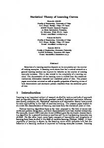
Figure 1. Dependence of wind-wave growth rate on nondimensional frequency ωU10 /g in log- and linear scales given by different experimental parameterizations (see legends).

The basic Kolmogorov constants Cp , Cq determine dependence of spectral levels on spectral flux quite like the case of river flow: the flux is higher – the water level is higher. The stationary solutions (11,12) seem to be unrealistic. First, they provide a transport between two infinities (from infinitely long to infinitely short waves for direct cascading and in an opposite sense for inverse cascading). Secondly, these solutions are isotropic while wind sea is strongly anisotropic. At the same time, the power-law tails of the unrealistic solutions are reproduced fairly well in all observations of wind sea. Further we give an explanation of this fact. 2.2. Wave input. Ocean field experiments give no direct way to discriminate wave generation or dissipation and to quantify experimentally nonlinear transfer term Snl which is co-existing with Sin , Sdiss [29]. To resolve this problem, heuristical models for Sin , Sdiss are widely used [14] as work-pieces for further parameterizing the observed wave input and dissipation. The Cherenkov-like formula is widely used in a majority of the wave input quasi-linear terms Sin [30, 17, 7, 29, 32, 18] (13)

Sin = β(k, Nk )Nk

where growth rate β(k) takes a form (14)

β(k) = ϱω(k)(ς − 1)n at ς > 1

and has an order of small parameter ϱ in (1). The Cherenkov-like factor (15)

ς=s

Uh cos θ Cph

relates a reference wind speed to the phase speed of wave harmonic( s is a coefficient close to 1, angle θ is related to wind direction). Waves moving slower than wind gain energy while waves which are faster than wind do not. Exponent n in (14) usually takes values 1 or 2. Details on parameterizing Sin can be found in [5] cited above. Here we just refer to figure 1 as an illustration of high dispersion of results given by different parametric formulas.

6

SERGEI I. BADULIN

2.3. Wave dissipation. Wave dissipation is the most poorly understood term in the kinetic equation (4). The quasi-linear parameterization of whitecapping mechanism by [14] is still the main model implemented in most of the the windwave forecasting models. Alternative saturation-based whitecapping formulations have been proposed in [1, 34]. Some other essentially nonlinear parameterizations of the term Sdiss [28, 7] are discussed predominantly in the context of research models. Some problems of the original whitecapping parameterization were demonstrated by [21] for the balance of fully developed wind-driven sea. Nowadays, spectral windwave models use this parameterization in the following form [ ( ω )4 ] Cdiss 2p+1 p/2 ( ω )2 F (f, θ) (16) Sdiss (f, θ) = − p ω ¯ m0 δ + (1 − δ) g ω ¯ ω ¯ where mean frequency ω ¯ is defined as (∫ +∞ ∫ (17) ω ¯=E×

(18)

ω

−1

)−1 E(ω, θ)dωdθ

,

−π

0

for total wave energy

π

∫

+∞

∫

π

E=

E(ω, θ)dωdθ. 0

−π

Cdiss = 4.5 and δ = 0.5 are default values in the WAM-cycle 4 model [10, 20] where the exponent p = 4 is usually used. Recent studies [41, 22] rely on much √ sharper, threshold-like dependence of the dissipation on wave steepness µ = ω ¯ E/g, with p > 10. According to [41], the whitecapping dissipation is overestimated in the WAM-cycle 3 and WAM-cycle 4 models. They propose to use the dissipation term (16) with the following parameters: Cdiss = 0.11, δ = 0 and p = 12. The key message of such revision is high exponent p that models threshold-like dependence of dissipation on wave steepness µ. Note a feature of formula (16) that makes it, in a sense, ‘non-physical’: it does not contain explicitly any small physical parameter while, logically, the term Sdiss should be of the same order of value as other terms of the right-hand side of the kinetic equation (4). In our opinion, the dissipation term (16) should be regarded simply as a tuning formula for poorly determined physical term. 3. Self-similarity of wind driven seas In this section we consider a way to resolve the problem of poorly determined terms Sin and Sdiss . The happy chance is in a fact that the term of non-linear transfer Snl appears to be the leading one in the right-hand side of (4). 3.1. On leading role of nonlinear transfer. As mentioned above the nonlinear interaction term Snl can be derived from the first principles. According to [38] it can be written as (19)

Snl = Fk − Γk Nk

where ‘nonlinear forcing’ Fk and ‘nonlinear damping’ Γk Nk ∫ Fk = πg 2 |T0123 |2 N1 N2 N3 δk+k1 −k2 −k3 δωk +ω1 −ω2 −ω3 dk1 dk2 dk3 ∫ Γk = πg 2 |T0123 |2 (N1 N2 + N1 N3 − N2 N3 )δk+k1 −k2 −k3 δωk +ω1 −ω2 −ω3 dk1 dk2 dk3

STATISTICAL THEORY OF WIND-WAVES

7

3 −2

10 2

1 −4

0

γ/ω

S*

nl

10

−1

−6

10

Γnl Γ th γ Snyder γDonelan γHsiaoShemdin

−2

−3 0

−8

0.5

1

1.5 ω/ωp

2

2.5

3

10

10

0

ω/ω

p

Figure 2. a) – Decomposition of the collision integral Snl (solid line) for the case by Komen et al. [21] into nonlinear forcing Fk (dashed) and damping Γk (dotted) terms; b) – Nonlinear damping coefficient Γk given by theoretical estimate (20) and by the numerical simulation (dashed and solid bold curves, correspondingly). Conventional dependencies of wind growth increments [30, 7, 17] are shown by thin curves with authors’ names in legend. Kernel Tk,k1 ,k2 ,k3 = Tk1 ,k,k2 ,k3 = Tk,k1 ,k3 ,k2 = Tk2 ,k3 ,k,k1 is a homogeneous function of order 3, invariant with respect to rotation. Collection of its explicit (and very complicated) expressions can be found in [3]. In the most real simulations Fk ≫ |Snl | and |Γk Nk | ≫ |Snl |. These two great components of Snl almost compensate each other. The Hasselmann equation in the form (19) shows a strong relaxation due to four-wave interactions ‘by itself’ in absence of any external forcing. Thus, one should compare input and dissipation terms not with the total Snl but with its separate components. In particular, one has to compare the total source growth rate γk = γin − γdiss with the decrement of nonlinear dissipation Γk generated by four-wave nonlinear interactions. For infinitely narrow spectrum one can obtain very simple estimate (20)

3

Γk = 36πω (ω/ωp ) µ4 cos2 Θ

that includes a huge enhancing factor: 36π ≈ 113.1. A representative estimate of wind input increment by Plant [29] gives ( )2 ( )2 U10 ωp ω −5 (21) γin = 5.1 · 10 ω g ωp where U10 – wind speed at standard height 10 meters above the sea surface. Two independent parameters – steepness µp and wind speed U10 determine the answer on relative balance of wave generation and nonlinear transfer. For the ratio of the linear input and nonlinear damping one gets from (20) (22)

−2

Γk /γin ≈ 2.26 · 105 (ω/ωp ) µ4p (U10 ωp /g)

Let for estimates in (22) the formally minimal value ω/ωp = 1 and U10 ωp /g = 2. Even for the most aggressive wave input by Plant [29] and rather young wind sea the nonlinear damping appears to be stronger than wind input for rather quiet sea (µp > 0.0365).

8

SERGEI I. BADULIN

3.2. Split balance model and weakly turbulent laws of wind wave growth. The fact of leading role of nonlinear transfer allows for constructing quite consistent asymptotic theory of wind-wave growth – the so-called split balance model [3]. In the lowest order of the theory the wave evolution is governed by the nonlinear transfer only dNk (23) = Snl dt The conservative kinetic equation (23) requires a boundary condition to determine a unique solution. The formally small terms of external forcing (wave input and dissipation) allows for formulating such condition in the form of balance of integral quantities d⟨Nk ⟩ = ⟨Sin + Sdiss ⟩ dt For deep water waves when the collision integral Snl is homogeneous function of wave vector one can construct a family of self-similar solutions. These solutions can be found for two particular cases: duration-limited (spatially homogeneous growth) and fetch-limited (stationary spatial growth) when total input ⟨Sin +Sdiss ⟩ is a power-law function of duration or fetch. These solutions have forms of selfsimilarity of the second type when spectral shape is determined by an ‘internal’ self-similar variable – non-dimensional frequency ω/ωp and ‘external’ dependence is specified by a power-law dependence on fetch or duration. Note, that it is consistent with conventional parameterizations of wind wave spectra, e.g. JONSWAP spectrum [15] and its modifications [6]. While in these widely used experimental parameterizations the second self-similar argument is wave age Cp /Uh , i.e. (24)

(25)

E(ω) = (Cp /Uh )κ Φ(ω/ωp )

the self-similar solutions of the split balance model (23, 24) do not contain wind speed explicitly. The key ‘external’ self-similar argument of these solutions is determined by total wave input ⟨Sin +Sdiss ⟩ – spectral flux at infinitely high frequencies. The relationship between the spectral magnitude (total energy) and the the total input appears to be similar to the links for the stationary Kolmogorov-Zakharov solutions (11,12. Thus, the split balance model allows to propose weakly turbulent law of wind-wave growth in the following form )1/3 ( Eωp4 ωp3 dE/dt (26) = αss g2 g2 Self-similarity parameter αss in (26) – an evident analogue of the Kolmogorov constants Cp , Cq in (11,12) depends slightly on exponents of self-similar solutions. Its numerical estimates are close to αss = 0.67 ± 0.1 [8]. Formally, the law (26) is valid for cases with power-law dependence of total input ⟨Sin + Sdiss ⟩ on duration or fetch. This validity has been demonstrated for more than 20 experimantal dependencies of wind wave growth [2]. It can be used as well in general case as an adiabatical relationship. 3.3. Reference cases of wind-wave growth. The split balance model in the form (23,24) does not consider explicitly wind-wave coupling operating with a total net wave input only. At the same time, important results on the coupling can be obtained using the weakly turbulent law of wave growth (26). Analysis of self-similar

STATISTICAL THEORY OF WIND-WAVES

9

solutions of the split balance model predicts a family of power-law dependencies for total energy and peak frequency on non-dimensional fetch χ (27a)

˜ = E0 χpχ ; E

ω ˜ p = ω0 χ−qχ

or non-dimensional duration τ (27b)

˜ = E 0 τ pτ ; E

ω ˜ p = ω0 τ −qτ

Three sets of exponents pχ(τ ) , qχ(τ ) in (27) play special role. These exponents correspond to one-parametric dependencies of wave height on wave period H ∼ Tz with exponents z = 5/3 [16], z = 3/2 [33], z = 4/3 [43]. The most known Toba’s 3/2 law [33] being treated within the weakly turbulent law (26) shows stationarity of net energy input dE/dt = const. Using the Toba law in the form (28)

Hs = B(gu∗ )1/2 Ts3/2

one can have from (26) immediately the energy rate (29)

dE π 9 B 6 u3∗ ρa u3∗ = = 0.16 . 3 g 3 g dt 8αss ρw αss

where B = 0.062 is the Toba constant [33]. Similarly, two other laws are consistent with weakly turbulent law of wind wave growth (26). It is easy to show that these cases correspond to stationarity of wave input of wave momentum [16, law 5/3] and wave action [43, law 4/3]. Estimates of energy input give the following parameterizations: (30)

dE ρa Cp u2∗ = 7.7 × 10−3 3 g dt ρw αss

for regime of constant in time production of wave momentum. Note, that the wave momentum can be associated quite naturally with turbulent wind stress τw = ⟨u′ w′ ⟩. The evolution of relatively old wind waves is provided by constant production of wave action an is decaying with wave age. (31)

dE ρa Cp−1 u4∗ = 1.6 3 g dt ρw αss

Summarizing results of the section emphasize one more fruitfulness of general approach to the problem. Further we consider two particular cases of wave evolution where the general analysis leads to interesting results. 4. The theory of wave turbulence and wind-wave forecasting The theory and forecasting of waves develop, to a considerable degree, independently. In addition to theoretical basics the wave forecasting uses extensively advanced technologies of data assimilation, remote and in situ measurements. In many cases, these technologies forced out the physically consistent modeling. Two cases given below show how a correct theoretical vision of wave growth can help in physical analysis and in improvement the wind wave forecasting.

10

SERGEI I. BADULIN 90 90

5

5

90

60

120 60

120

2.5

150

2.5

k

180

210

210

240 300

0

330

330

270

30

0

0

240

2.5

150

180

180

210

60

30

30

y

150

5

120

330

300 270 k x

240

300 270

Figure 3. Evolution of spatial spectrum of mixed wave field. Left – initial state at t = 0 with two peaks at periods about 10 (swell) and 5 (locally generated wind waves) seconds. Swell propagates at angle 30◦ to the wind direction. Center – wave spectrum at t = 522 sec. (approximately 100 periods of wind waves. Right – t = 2000 sec., wind waves are almost completely absorbed by swell. 4.1. Example 1: anomalously strong relaxation in the mixed sea. Usually wave field in the ocean is a superposition of waves generated by local wind and of remotely generated swell. This case, the so-called mixed sea, is of special theoretical and practical interest. Special methods are developed for discriminating the observed wave field into two components: wind waves and swell. Theoretical description of the state is also not trivial as far swell and wind waves evolve at essentially different spatio-temporal scales and the physical mechanisms of their coupling with wind are also quite different. Very interesting effects can be associated with the mixed sea state [25]. Some of these effects described in [36, 19, 27] can be treated adequately within the presented statistical approach and the concept of dominating nonlinear transfer. In figures 3 results of numerical simulation of the mixed wind sea are presented. Initial two-mode spectrum consists of a strong swell with period about 10 seconds and relatively weak wind component with period 5 seconds. Anomalously fast relaxation of wind-driven components is clearly seen at timescale of first hundreds of wave periods. This timescale can be estimated adequately by formula (20): The effect of low frequency swell enhances relaxation by non-dimensional factor ω/ωp , while steep young wind waves gives additional effect by factor µ4p . As a result, the anomalously fast absorption of wind waves by swell occurs. These effects were reported in [27, 19] for Baltic Sea where wind waves follow preferential directions associated with propagation of swell. 4.2. Example 2: wind waves in Tallinn Bay. As the second example of adequate use of the statistical approach consider the regional wave model developed for Tallinn Bay in Tallinn University of Technology [31]. This model was created on the basis of an international standard of wave forecasting models – WAM (Wave) [20]. The construction of any wave model for such small basin as Tallinn Bay is accompanied by a number of question. The first one is on adequacy of the statistical approach itself for the case when spatial scales numbers a few hundred of wavelengths. Fortunately, it works in a majority of cases quite well. Two assumptions accepted in [31] take into account specific physics of wind wave field. First, Wind

STATISTICAL THEORY OF WIND-WAVES

11

field is considered as homogeneous in the bay and is not affected by remote wave field. The second one is not so evident but it allows to predict wave field quite good at reasonable computational efforts: the wave field is considered as independent on previous history, as a sort of saturated state. The model showed its ability for analysis of long-term and climatic features in the closed basin of Tallin Bay. Implicitly, the success of this modelling justify our above conclusions: the relaxation of wave field due to nonlinear wave-wave interactions is quite strong. The details of wave input and dissipation appear to be of secondary importance. 5. Concluding remarks In this lecture we presented ideas rather than ready-to-use recipes and recommendations for modeling wave field in near-shore zone. At the same time asymptotic split balance model has been given as a tool of transparent physical analysis. Basing on hypothesis of dominating nonlinear transfer we obtained explicit formulas for the rate of nonlinear damping (20) and estimates of wave input due to wind (29,30,31). Examples of the last section show adequacy of these simple relationships. The list of references is essential part of this lecture and should be used for further progress in wave studies. Our lecture shows that in the near-shore dynamics in not a collection of a great number of methods, physical factors etc. It can contain, as in case of wave studies, surprisingly transparent physics and, thus, is very attractive for young researchers.

References [1] J. H. G. M. Alves and M. L. Banner, Performance of a saturation-based dissipation-rate source term in modeling the fetch-limited evolution of wind waves, JPO 33 (2003), 1274– 1298. [2] S. I. Badulin, A. V. Babanin, D. Resio, and V. Zakharov, Weakly turbulent laws of wind-wave growth, J. Fluid Mech. 591 (2007), 339–378. [3] S. I. Badulin, A. N. Pushkarev, D. Resio, and V. E. Zakharov, Self-similarity of wind-driven seas, Nonl. Proc. Geophys. 12 (2005), 891–946. [4] B. B.Kadomtsev, Collective phenomena in plasma, Nauka, Moscow,, 1976, 238 p. [5] L. Cavaleri, J.-H. G. M. Alves, F. Ardhuin, A. Babanin, M. Banner, K. Belibassakis, M. Benoit, M. Donelan, J. Groeneweg, T. H. C. Herbers, P. Hwang, P. A. E. M. Janssen, T. Janssen, I. V. Lavrenov, R. Magne, J. Monbaliu, M. Onorato, V. Polnikov, D. Resio, W. E. Rogers, A. Sheremet, J. McKee Smith, H. L. Tolman, G. van Vledder, J. Wolf, and I. Young, Wave modelling – the state of the art, Progr. Ocean. 75 (2007). [6] M. Donelan, M. Skafel, H. Graber, P. Liu, D. Schwab, and S. Venkatesh, On the growth rate of wind-generated waves, Atmosphere Ocean 30 (1992), no. 3, 457–478. [7] M. A. Donelan and W. J. Pierson-jr., Radar scattering and equilibrium ranges in windgenerated waves with application to scatterometry, J. Geophys. Res. 92 (1987), no. C5, 4971– 5029. [8] E. Gagnaire-Renou, M. Benoit, and S. I. Badulin, On weakly turbulent scaling of wind sea, JFM (2010), submitted. [9] E. Gagnaire-Renou, M. Benoit, and P. Forget, Ocean wave spectrum properties as derived from quasi-exact computations of nonlinear wave-wave interactions, JGR (2010), no. doi:10.1029/2009JC005665. unther, K. Hasselmann, and P. A. E. M. Janssen, The WAM model Cycle 4 (revised [10] H. G¨ version), Tech. Rep. 4. Deutsch. Klimatol. Rechenzentrum, Hamburg, Germany (1992), no. 4 (English). [11] K. Hasselmann, On the nonlinear energy transfer in a gravity wave spectrum. Part 1. General theory, J. Fluid Mech. 12 (1962), 481–500 (English).

12

[12]

[13] [14] [15]

[16] [17] [18] [19] [20] [21] [22]

[23] [24] [25]

[26] [27] [28] [29] [30] [31] [32] [33] [34] [35] [36] [37]

SERGEI I. BADULIN

, On the nonlinear energy transfer in a gravity wave spectrum. evaluation of the energy flux and swell-sea interaction for a neumann spectrumP. 3, J. Fluid Mech. 15 (1963), 385–398 (English). , On the nonlinear energy transfer in a gravity wave spectrum. Part 2 Conservation theorems; wave-particle analogy; irreversibility., J. Fluid Mech. 15 (1963), 273–281 (English). , On the spectral dissipation of ocean waves due to white capping, Boundary-Layer Meteorol. 6 (1974), 107–127 (English). K. Hasselmann, T. P. Barnett, E. Bouws, H. Carlson, D. E. Cartwright, K. Enke, J. A. Ewing, H. Gienapp, D. E. Hasselmann, P. Kruseman, A. Meerburg, P. Muller, D. J. Olbers, K. Richter, W. Sell, and H. Walden, Measurements of wind-wave growth and swell decay during the Joint North Sea Wave Project (JONSWAP), Dtsch. Hydrogh. Zeitschr. Suppl. 12 (1973), no. A8. K. Hasselmann, D. B. Ross, P. M¨ uller, and W. Sell, A parametric wave prediction model, J. Phys. Oceanogr. 6 (1976), 200–228. S. V. Hsiao and O. H. Shemdin, Measurements of wind velocity and pressure with a wave follower during MARSEN, J. Geophys. Res. 88 (1983), no. C14, 9841–9849. P. A. E. M. Janssen, Wave-induced stress and the drag of air flow over sea waves, J. Phys. Oceanogr. 19 (1989), 745–754 (English). K. K. Kahma and H. Pettersson, Wave growth in a narrow fetch geometry, Global Atmos. Ocean Syst. 2 (1994), 253–263. G. J. Komen, L. Cavaleri, M. Donelan, K. Hasselmann, S. Hasselmann, and P. A. E. M. Janssen, Dynamics and modelling of ocean waves, Cambridge University Press, 1995. G. J. Komen, S. Hasselmann, and K. Hasselmann, On the existence of a fully developed wind-sea spectrum, J. Phys. Oceanogr. 14 (1984), 1271–1285 (English). A. O. Korotkevich, A. N. Pushkarev, D. Resio, and V. E. Zakharov, Numerical verification of the weak turbulent model for swell evolution, Eur. J. Mech. B/Fluids 27 (2008), no. 361, doi:10.1016/j.euromechflu.2007.08.004. V. P. Krasitskii, On reduced Hamiltonian equations in the nonlinear theory of water surface waves, J. Fluid Mech. 272 (1994), 1–20 (English). J. Lighthill, Waves in fluids, Cambridge University Press, Cambridge, United Kingdom, 1978, 504 p. Dung Nguy, Observations on the directional on the directional development of wind-waves in mixed seas, Master of science in mechanical engineering, University of Washington, 1998, Technical report APL-UW-TR9802. L. W. Nordheim, On the kinetic method in the new statistics and its applications in the electron theory of conductivity, Proc. Roy. Soc. Lond. A 119 (1928), 689–698 (English). Heidi Pettersson, Wave growth in a narrow bay, Ph.D. thesis, University of Helsinki, 2004, [ISBN 951-53-2589-7 (Paperback) ISBN 952-10-1767-8 (PDF)]. O. M. Phillips, Spectral and statistical properties of the equilibrium range in wind-generated gravity waves, J. Fluid Mech. 156 (1985), 505–531 (English). W. J. Plant, A relationship between wind stress and wave slope, J. Geophys. Res. 87 (1982), no. C3, 1961–1967. R. L. Snyder, F. W. Dobson, J. A. Elliot, and R. B. Long, Array measurements of atmospheric pressure fluctuations above surface gravity waves, J. Fluid Mech. 102 (1981), 1–59 (English). T. Soomere, Wind wave statistics in Tallinn Bay, Boreal Env. Res. 10 (2005), 103–118 (English). R. W. Stewart, The air-sea momentum exchange, Boundary-Layer Meteorol. 6 (1974), 151– 167 (English). Y. Toba, Local balance in the air-sea boundary processes. I. on the growth process of wind waves, J. Oceanogr. Soc. Japan 28 (1972), 109–121. A. J. Van der Westhuysen, M. Zijlema, and J. A. Battjes, Nonlinear saturation-based whitecapping dissipation in swan for deep and shallow water, CE 454 (2007), 151–170. G. B. Whitham, Linear and nonlinear waves, Wiley, New York, 1974, 636 p. I. R. Young, Directional spectra of hurricane wind waves, J. Geophys. Res. 111 (2006), doi:10.1029/2006JC003540. V. E. Zakharov, Problems of the theory of nonlinear surface waves, Ph.D. thesis, Budker Institute for Nuclear Physics, Novosibirsk, USSR, 1966.

STATISTICAL THEORY OF WIND-WAVES

[38] [39] [40] [41] [42]

[43]

13

, Statistical theory of gravity and capillary waves on the surface of a finite-depth fluid, Eur. J. Mech. B/Fluids 18 (1999), 327–344 (English). V. E. Zakharov, G. Falkovich, and V. Lvov, Kolmogorov spectra of turbulence. part I, Springer, Berlin, 1992 (English). V. E. Zakharov and N. N. Filonenko, Energy spectrum for stochastic oscillations of the surface of a fluid, Soviet Phys. Dokl. 160 (1966), 1292–1295 (English). V. E. Zakharov, A. O. Korotkevich, A. N. Pushkarev, and D. Resio, Coexistence of weak and strong wave turbulence in a swell propagation, Phys. Rev. Lett. 99 (2007), no. 164501. V. E. Zakharov and M. M. Zaslavsky, The kinetic equation and Kolmogorov spectra in the weak-turbulence theory of wind waves, Izv. Atmos. Ocean. Phys. 18 (1982), 747–753 (English). , Dependence of wave parameters on the wind velocity, duration of its action and fetch in the weak-turbulence theory of water waves, Izv. Atmos. Ocean. Phys. 19 (1983), no. 4, 300–306 (English).

P.P. Shirshov Institute of Oceanology, Moscow, Russia E-mail address: [email protected]