analytical chemistry, quantitative analysis, and introductory statistics. We'll
discuss and highlight statistical concepts most important to a forensic chemist on
a ...
Bell_Ch02v2.qxd 3/23/05 7:43 PM Page 13
CHAPTER
Statistics, Sampling, and Data Quality
2
2.1 Significant Figures, Rounding, and Uncertainty 2.2 Statistics for Forensic and Analytical Chemistry
O VER VIEW
AND
O RIENTATION
Data quality lies at the core of what forensic chemistry is and how forensic data are used. The goal of quality assurance and quality control (QA/QC) is to generate trustworthy laboratory data. There is an imperishable link between data quality, reliability, and admissibility. Courts should admit only trustworthy scientific evidence; ultimately, the courts have to rely on the scientific community for such evaluations. Rule 702 of the Federal Rules of Evidence states that an expert in a field such as chemistry or toxicology may testify about their results, “if (1) the testimony is based upon scientific facts or data, (2) the testimony is the product of reliable principles and methods, and (3) the witness has applied the principles and methods reliably to the facts of the case.” Quality assurance practices are designed to define reliability in a concrete and quantitative way. The quantitative connection is found in statistics, the subject of this chapter. By design and necessity, this is a brief treatment of statistics. It is meant as a review and supplement to your existing knowledge, not as a substitute for material presented in courses such as analytical chemistry, quantitative analysis, and introductory statistics. We’ll discuss and highlight statistical concepts most important to a forensic chemist on a daily basis. Quality assurance is dynamic, is evolving, and requires daily care and maintenance to remain viable. It is also a layered structure, as shown in Figure 2.1. At every level in the triangle, statistics provides the means for evaluating and judging data and methods. Without fundamental statistical understanding, there can be no quality management or assurance. Accordingly, we 13
Bell_Ch02v2.qxd 3/23/05 7:43 PM Page 14
14
Chapter 2 Statistics, Sampling, and Data Quality
• Continuing education • Reference materials • Standard methods • Quality standards • Peer review
External scientific organizations
• Laboratory accreditation • Continuing education • Analyst certification • Proficiency testing • Peer review • Audits
Professional organizations
Forensic laboratory
▲
Figure 2.1 The layered structure of quality assurance. Statistics underlies each level and stage.
• Training and continuing education • Equipment calibration • Standard procedures • Method validation • Internal QA/QC • Instrument logs • Control charts • Peer review
Reliable analytical data
• Analysis • Controls • Documentation • Data analysis • Reporting
will begin our exploration of quality assurance (QA) and statistics with a review of fundamental concepts dealing with uncertainty and significant figures. You may recall working problems in which you were asked to determine the number of significant figures in a calculation. Forensic and analytical chemistry gives us a context for those exercises and makes them real. We will start there and quickly make the link between significant figures and uncertainty. The idea of the inherent uncertainty of measurement and random errors will lead us into a review of the statistical concepts that are fundamental to forensic chemistry. The last part of the chapter centers on sampling statistics, something that forensic chemists must constantly be aware of. The information presented in this chapter will take us into a discussion of calibration, multivariate statistics, and general quality assurance and quality control in the next chapter.
2.1 S IGNIFICANT F IGURES , R OUNDING , AND U NCER TAINTY Significant figures become tangible in analytical chemistry. The concept of significant figures arises from the use of measuring devices and equipment and their associated uncertainty. How that uncertainty is accounted for dictates how to round numbers resulting from what may be a complicated series of laboratory procedures. The rules and practices of significant figures and rounding
Bell_Ch02v2.qxd 3/23/05 7:43 PM Page 15
2.1 Significant Figures, Rounding, and Uncertainty 15 must be applied properly to ensure that the data presented are not misleading, either because there is too much precision implied by including extra unreliable digits or too little by eliminating valid ones.1
Exhibit A: Why Significant Figures Matter In most states, a blood alcohol level of 0.08% is the cutoff for intoxication. How would a value of 0.0815 be interpreted? What about 0.07999? 0.0751? Are these values rounded off or are they truncated? If they are rounded, to how many significant digits? Of course, this is an artificial, but still telling, example. How numerical data are rounded depends on the instrumentation and devices used to obtain the data. Incorrect rounding might have consequences.
In any measurement, the number of significant digits is defined as the number of digits that are certain, plus one. The last digit is uncertain (Figure 2.2), meaning that it is an estimate, but a reasonable one. With the bathroom scale example, one person might interpret the value as 125.4 and another as 125.6, but it is certain that the value is greater than 125 pounds and less than 126. The same situation arises when you use rulers or other devices with calibrated marks. Digital readouts of many instruments may cloud the issue a bit, but unless you are given a defensible reason to know otherwise, assume that the last decimal on a digital readout is uncertain as well. Recall that zeros have special rules and may require a contextual interpretation. As a starting point, a number may be converted to scientific notation. If the zeros can be removed by this operation, then they were merely placeholders representing a multiplication or division by 10. For example, suppose an instrument produces a result of 0.001023 that can be expressed as 1.023 * 10-3. Then the leading zeros are not significant, but the embedded zero is. Trailing zeros can be troublesome. In analytical chemistry, the rule should be that if a zero is meant to be significant, it is listed, and conversely, if a zero is omitted, it was not significant. Thus, a value of 1.2300 grams for a weight means that the balance actually displayed two trailing zeros. It would be incorrect to record a balance reading of 1.23 as 1.2300. Recording that weight as 1.2300 is conjuring numbers that are useless at best and are very likely deceptive. If this weight were embedded in a series of calculations, the error would propagate, with potentially disastrous consequences. “Zero” does not imply “inconsequential,” nor does it imply “nothing.” In recording a weight of 1.23 g, no one would arbitrarily write 1.236, so why should writing 1.230 be any less onerous? In combining numeric operations, rounding should always be done at the end of the calculation.1 The only time that rounding intermediate values may be appropriate is in addition and subtraction operations, although caution must still be exercised. In such operations, the result is rounded to the same
▲
124 125 126 123
127 Uncertain 125.4 lbs 4 significant digits
Figure 2.2 Reading the scale results in four significant digits, the last being an educated guess or an approximation that, by definition, will have uncertainty associated with it.
Bell_Ch02v2.qxd 3/23/05 7:43 PM Page 16
16
Chapter 2 Statistics, Sampling, and Data Quality number of significant digits as there are in the contributing number with the fewest digits, with one extra digit included to avoid rounding error. For example, assume that a calculation requires the formula weight of PbCl2: Pb = 207.2 g/mole Cl = 35.4527 g/mole
207.2ƒ 2135.4272 = 70.8ƒ54 278.0ƒ54 g/mole
The correct way to round or report an intermediate value would be 278.05 rather than 278.1. The subscript indicates that one additional digit is retained to avoid rounding error. The additional digit does not change the count of significant digits: The value 278.05 still has four significant digits. The subscript notation is designed to make this clear. The formula weight should rarely, if ever, limit the number of significant digits in a combined laboratory operation. In most cases, it is possible to calculate a formula weight to enough significant figures such that the formula weight does not control rounding. Lead, selected purposely for the example, is one of the few elements that may limit significant-figure calculations. By definition, the last significant digit obtained from an instrument or a calculation has an associated uncertainty. Rounding leads to a nominal value, but it does not allow for expression of the inherent uncertainty. To do this, the uncertainties of each contributing factor, device, or instrument must be known and accounted for. For measuring devices such as analytical balances, Eppendorf pipets, and flasks, that value is either displayed on the device, supplied by the manufacturer, or determined empirically. Because these values are known, it is also possible to estimate the uncertainty (i.e., potential error) in any combined calculation. The only caveat is that the units must be the same. On an analytical balance, the uncertainty would be listed as ;0.0001 g, whereas the uncertainty on a volumetric flask would be reported as ;0.12 mL. These are absolute uncertainties that cannot be combined, as is because the units do not match. To combine uncertainties, relative uncertainties must be used. These can be expressed as “1 part per Á ” or as a percentage. That way, the units cancel and a relative uncertainty results, which may then be combined with other uncertainties expressed the same way (i.e., as unitless value). Consider the simple example in Figure 2.3, in which readings from two devices are utilized to obtain a measurement in miles per gallon. The absolute uncertainty of each device is known, so the first step in combining them is to express them as “1 part per Á ” While not essential, such notation shows at a glance which uncertainty (if any) will dominate. It is possible to estimate the uncertainty of the mpg calculation by assuming that the odometer uncertainty of 0.11% (the relative uncertainty) will dominate. In many cases, one uncertainty is much larger (two or more orders of magnitude) than the other and hence will control the final uncertainty. Better in this case is accounting for both uncertainties, because they are within an order of magnitude of each other (0.07% vs. 0.11%). Relative uncertainties are combined with the use of the formula et = 21e 21 + e 22 + e 23 + Á + e 2n2
(2.1)
For the example provided in Figure 2.3, the results differ only slightly when uncertainties are combined, because both were close to 0.1%, so neither overwhelms
Bell_Ch02v2.qxd 3/23/05 7:43 PM Page 17
2.2 Statistics for Forensic and Analytical Chemistry 17 Odometer (+/– 0.2 miles) 183.4 miles Absolute uncertainty Feul pump indicator 6.683 gallons (+/– 0.005 gallons) Absolute uncertainty MPG:
183.4 miles
=
27.44mpg
6.683 gallons Uncertanties: relative Odometer =
2 miles
=
183.4 miles Pump =
0.005 gal 6.683 gal
1 917
=
1 1337
% uncertainty ⫻ 100 = 0.11%*
⫻ 100 = 0.07%
Estimated: 0.11% of 27.44 mpg = 0.0302 = 0.30 Range = 27.44 +/– 0.030 = 27.41 — 27.47mpg
Propogated:
Range = 27.40 — 27.48mpg
the other. (Incidentally, the value e as given here is equivalent to a variance (v), a topic to be discussed shortly in Section 2.2.1.) Equation 2.1 represents the propagation of uncertainty. It is useful for estimating the contribution of instrumentation and measuring devices to the overall potential error. It cannot take other types of determinate errors into account, however. Suppose some amount of gasoline in the preceding example overflowed the tank and spilled on the ground. The resulting calculation is correct but not reliable. Spilling gasoline is the type of procedural error that is detected and addressed by quality assurance, the topic of the next chapter. In turn, quality assurance requires an understanding of the mathematics of multiple measurements, or statistics.
2.2 S TATISTICS FOR F ORENSIC AND A NALYTICAL C HEMISTRY 2.2.1 OVERVIEW AND DEFINITIONS The application of statistics requires replicate measurements. A replicate measurement is defined as a measurement of a criterion or value under the same experimental conditions for the same sample used for the previous measurement.
▲
C T = √(0.0011)2 + 0.0007)2 = 0.0013 = 0.13% 0.13% of 27.44 = 0.0357 = 0.036
Figure 2.3 Calculation of mpg based on two instrumental readings.
Bell_Ch02v2.qxd 3/23/05 7:43 PM Page 18
18
Chapter 2 Statistics, Sampling, and Data Quality
Example Problem 2.1 A drug analysis is performed with gas chromatography/mass spectrometry (GCMS) and requires the use of reliable standards. The lab purchases a 1.0-mL commercial standard that is certified to contain the drug of interest at a concentration of 1.00 mg/mL with an uncertainty of ;1.0%. To prepare the stock solution for the calibration, an analyst uses a syringe with an uncertainty of ;0.5% to transfer 250.0 mL of the commercial standard to a Class-A 250-mL volumetric flask with an uncertainty of ;0.08 mL. What is the final concentration and uncertainty of the diluted calibration stock solution?
Answer:
Commercial standard 1.00 mg + /– 1.07% mL
Syringe
Volumetric flask
Relative uncertainty
Relative uncertainty
= 0.5
Relative uncertainty = 0.010
0.08 mL
= 0.005
100
250.0 mL
To calculate the concentration: Concentrated C1V1
Diluted =
C2V2
1.00 mg 0.250 mL mL
C2 =
C2 =
?
(100mLmg ) ( 0.250 mL) 250.0 mL 1.00 mg mL
=
1000 mg L
=
250.0 mL
0.00100 mg mL
= 1000 ppb
et = √(0.010)2 + 0.005)2 + 0.0003)2 = 0.01 Stock concentration = 10.00 ppb +/– 10 ppb
= 0.0003
Bell_Ch02v2.qxd 3/23/05 7:43 PM Page 19
2.2 Statistics for Forensic and Analytical Chemistry 19 0.4
0.3
0.1
0
Figure 2.4 A Gaussian distribution. Most measurements cluster around the central value (the mean) and decrease in occurrence the farther from the mean. “Frequency” refers to how often a measurement occurs; 40% of the replicate measurements were the mean value, with frequency 0.4.
▲
0.2
–
0 Deviation from mean
+
That measurement may be numerical and continuous, as in determining the concentration of cocaine, or categorical (yes/no; green/orange/blue, and so on). We will focus attention on continuous numerical data. If the error associated with determining the cocaine concentration of a white powder is due only to small random errors, the results obtained are expected to cluster about a central value (the mean), with a decreasing occurrence of values farther away from it. The most common graphical expression of this type of distribution is a Gaussian curve. It is also called the normal error curve, since the distribution expresses the range of expected results and the likely error. It is important to note that the statistics to be discussed in the sections that follow assume a Gaussian distribution and are not valid if this condition is not met. The absence of a Gaussian distribution does not mean that statistics cannot be used, but it does require a different group of statistical techniques. In a large population of measurements (or parent population), the average is defined as the population mean m. In most measurements of that population, only a subset of the parent population (n) is sampled. The average value for that subset (the sample mean, or x) is an estimate of m. As the number of measurements of the population increases, the average value approaches the true value. The goal of any sampling plan is twofold: first, to ensure that n is sufficiently large to appropriately represent characteristics of the parent population; and second, to assign quantitative, realistic, and reliable estimates of the uncertainty that is inevitable when only a portion of the parent population is studied. Consider the following example (see Figure 2.5), which will be revisited several times throughout the chapter: As part of an apprenticeship, a trainee in a forensic chemistry laboratory is tasked with determining the concentration of cocaine in a white powder. The powder was prepared by the QA section of the laboratory, but the concentration of cocaine is not known to the trainee (who has a blind sample). The trainee’s supervisor is given the same sample with the same constraints. Figure 2.5 shows the result of 10 replicate analyses 1n = 102 made by the two chemists. The supervisor has been performing such analyses for years, while this is the trainee’s first attempt. This bit of information is important for interpreting the results, which will be based on the following quantities now formally defined: The sample mean 1x2: The sample mean is the sum of the individual measurements, divided by n. Most often, the result is rounded to the same
Bell_Ch02v2.qxd 3/23/05 7:43 PM Page 20
20
Chapter 2 Statistics, Sampling, and Data Quality True value
▲
Figure 2.5 Hypothetical data for two analysts analyzing the same sample 10 times each, working independently. The chemists tested a white powder to determine the percent cocaine it contained. The true value is 13.2%. In a small data set 1n = 102, the 95% CI would be the best choice, for reasons to be discussed shortly. The absolute error for each analyst was the difference between the mean that analyst obtained and the true value.
Sample 1 2 3 4 5 6 7 8 9 10
% Error Mean Standard error Standard deviation (sample) %RSD (CV) (sample) Standard deviation (population) %RSD (CV) (population) Sample variance Range Confidence level (95.0%) 95% Cl range
13.2% +/– 0.1% Trainee 12.7 13.0 12.0 12.9 12.6 13.3 13.2 11.5 15.0 12.5
Forensic chemist 13.5 13.1 13.1 13.2 13.4 13.1 13.2 13.7 13.2 13.2
Trainee –2.5 12.9 0.29 0.93 7.2 0.88 6.8 0.86 3.5 0.66 12.2–13.6
Forensic chemist 0.5 13.3 0.06 0.20 1.5 0.19 1.4 0.04 0.6 0.14 13.2–13.4
number of significant digits as in the replicate measurements.1 However, occasionally an extra digit is kept, to avoid rounding errors. Consider two numbers: 10. and 11. What is the sample mean? 10.5, but rounding would give 10, not a terribly helpful calculation. In such cases, the mean can be expressed as 10.5, with the subscript indicating that this digit is being kept to avoid or address rounding error. The 5 is not significant and does not count as a significant digit, but keeping it will reduce rounding error.1 Having said that, in many forensic analyses rounding to the same significance as the replicates is acceptable and would be reported as shown in Figure 2.5. The context dictates the rounding procedures. In this example, rounding was to three significant figures, given that the known has a true value with three significant figures. The rules pertaining to significant figures may have allowed for more digits to be kept, but there is no point to doing so on the basis of the known true value and how it is reported. Absolute error: This quantity measures the difference between the true value and the experimentally observed value with the sign retained to indicate how the results differ. For the trainee, the absolute error is calculated as 12.9 - 13.2, or -0.3% cocaine. The negative sign indicates that the trainee’s calculated mean was less than the true value, and this information is useful in diagnosis and troubleshooting. For the forensic chemist, the absolute error is 0.1 with the positive indicating that the experimentally determined value was greater than the true value. % Error: While the absolute error is a useful quantity, it is difficult to compare across data sets. An error of -0.3% would be much less of a concern if the true value of the sample was 99.5% and much more of a concern if the true value was 0.5%. If the true value of the sample was indeed 0.5%, an absolute error of 0.3% translates to an error of 60%. To address this limitation of absolute error, the % error is employed. This quantity normalizes the absolute error to the true value: % error = [1experimentally determined value - true value2/true value]*100
(2.2)
Bell_Ch02v2.qxd 3/23/05 7:43 PM Page 21
2.2 Statistics for Forensic and Analytical Chemistry 21
Exhibit B: Statistics “Cheat Sheet” Population
Sample
N Population mean, m Population standard deviation, s
n Sample mean, x Sample standard deviation, s
Relative frequency (probability) of occurance of measurement
0.4
0.3 Equation of a Gaussian Curve 0.2
(x – ) z/2
y=
0.1
e /√2
0
Magnitude of measurement, x
–
0
+
Error of measurement, x –
–3
–2
–1
0
1
2
3
Standardized variable, z = (x – )/
68.27% of measurement in this range
95.45% of measurement in this range
Only 0.27% of measurement outside this range
For the trainee, the % error is -2.5% whereas for the forensic chemist, it is 0.5%. The percent error is commonly used to express the accuracy of an analysis when the true value is known. The technique of normalizing a value and presenting it as a percentage will be used again for expressing precision (reproducibility), to be described next. The limitation of % error is that this quantity does not take into account the spread or range of the data. A separate quantity
Bell_Ch02v2.qxd 3/23/05 7:43 PM Page 22
22
Chapter 2 Statistics, Sampling, and Data Quality
Relative frequency
0.4
–A
A
+A
B
B
B
0.3 0.2 0.1 0
–2B
–2A +2A
+2B
– + 0 Deviation from mean, x –
▲ Figure 2.6 Two Gaussian distributions centered about the same mean, but with a different spread (standard deviation). This approximates the situation with the forensic chemist and the trainee.
is used to characterize the reproducibility (spread) and to incorporate it into the evaluation of experimental results. Standard deviation: The standard deviation is the average deviation from the mean and measures the spread of the data. (See Figure 2.6.) The standard deviation is typically rounded to two significant figures.1 A small standard deviation means that the replicate measurements are close to each other; a large standard deviation means that they are spread out over a larger range of values. In terms of the normal distribution, ;1 standard deviation from the mean includes approximately 68% of the observations, ;2 standard deviations includes about 95%, and ;3 standard deviations includes around 99%. A large value for the standard deviation means that the distribution is wide; a small value for the standard deviation means that the distribution is narrow. The smaller the standard deviation, the closer is the grouping and the smaller is the spread. In other words, the standard deviation measures reproducibility of the measurements. The experienced supervisor produced data with more precision (less of a spread) than that produced by the trainee, as would be expected based on their skill levels. In Figure 2.5, two values are reported for the standard deviation: that of the population 1s2 and that of the sample (s). The population standard deviation is calculated as N
s =
2 a 1xi - m2
i=1
S
n
(2.3)
where i is the number of replicates, 10 in this case.† Ten replicates is a relatively small number compared with 100, 1000, or an infinite number, as would be required to obtain the true value m. The value s is the standard deviation of the parent population. The use of s with small sample sets underestimates the true standard deviation s.2 A statistically better estimate of s is given by: n
s =
a axi - xb
i=1
S
n - 1
2
(2.4)
The value of s is the standard deviation of the selected subset of the parent population. Some calculators and spreadsheet programs differentiate between s and s, so it is important to make sure that the correct formula is applied. The sample standard deviation(s) provides an empirical measure of uncertainty (i.e., expected error) and is frequently used for that purpose. If a distribution is normal, 68.3% of the values will fall between ;1 standard deviation 1;1s2, 95.4% within 2s, and 99.7% within ;3s from the mean. This concept is shown in Figure 2.7. This spread provides a range of measurements as well as a probability of occurrence. Most often, the uncertainty is cited as ;2 standard deviations, since approximately 95% of the area under the normal distribution curve is contained within these boundaries. Sometimes ;3 standard deviations are used, to account for more than 99% of the area under the curve. Thus, if the †
Although s is based on sampling the entire population, it is sometimes used in forensic and analytical chemistry. One rule of thumb is that if n 7 15, population statistics may be used. Similarly, if all samples in a population are analyzed, population statistics are appropriate. For example, to determine the average value of coins in a jar full of change, every coin could be included in the sampling and population statistics would be appropriate.
Bell_Ch02v2.qxd 3/23/05 7:43 PM Page 23
2.2 Statistics for Forensic and Analytical Chemistry 23 a.
0.5 0.4 0.3 y 0.2
0.683
0.1 0 –4 b.
–3
–2
–1
0 x
1
2
3
4
0.5
0.4
0.3 y 0.2
0.954
0.1
0 –4
c.
–3
–2
–1
0 x
1
2
3
4
0.5
0.4
▲
0.3 y 0.2
0.997
0.1
0 –4
–3
–2
–1
0 x
1
2
3
4
distribution of replicate measurements is normal and a representative sample of the larger population has been selected, the standard deviation can be used to reliably estimate an uncertainty. As shown in Table 2.1, the supervisor and the trainee both obtained a mean value within ;0.3% of the true value. When uncertainties associated with the standard deviation and the analyses are considered, it becomes clear that both obtained an acceptable result. This is also seen graphically in Figure 2.8. However, the trainee would likely be asked to practice and try again, not because of
Figure 2.7 Area under the Gaussian curve as a function of standard deviations from the mean. Within one standard deviation (a), 68.3% of the measurements are found; 95.4% (b) are found within two standard deviations, and (c) 99.7% are found within three standard deviations.
Bell_Ch02v2.qxd 3/23/05 7:43 PM Page 24
24
Chapter 2 Statistics, Sampling, and Data Quality Table 2.1 Comparison of Ranges for Determination of Percent Cocaine in QA Sample, m = 13.2% Calculation Method
Trainee, x = 12.9
Min–Max ;1s ;2s ;3s 95% CI
11.5–15.0 12.0–13.8 11.0–14.8 10.1–15.7 12.2–13.6
Forensic Chemist, x = 13.3 13.1–13.7 13.1–13.4 12.9–13.7 12.7–13.9 13.2–13.4
the poor accuracy, but because of the poor reproducibility. In any laboratory analysis, two criteria must be considered: accuracy (how close the result is to the true value) and precision (how reproducible the result is). One without the other is an incomplete description. Variance (v): The sample variance (v) of a set of replicates is simply s2, which, like the standard deviation, gauges the spread, expected error, or variance within that data set. Forensic chemists favor standard deviation as their primary measure of reproducibility, but variance is used in analysis-of-variance (ANOVA) procedures as well as in multivariate statistics. Variances are additive and are the basis of error propagation, as seen in equation (2.1), where the variance was represented by e 2. %RSD of coefficient of variation (CV or %CV): The standard deviation alone means little and doesn’t reflect the relative or comparative spread of the data. This situation is analogous to that seen with the quantity of absolute error. To compare the spread (reproducibility) of one data set with another, the mean must be taken into account. If the mean of the data is 500 and the standard deviation is 100, that’s a relatively large standard deviation. By contrast, if the mean of the data is 1,000,000, a standard deviation of 100 is relatively tiny. The significance
+/– 3S +/– 2S Trainee
95% CI +/– 1S
Absolute error = – –x
11.0 Sample
12.0
12.8 13.0
13.4 13.6
14.0
+/– 3S
▲
Figure 2.8 Results of the cocaine analysis presented graphically with uncertainty reported several ways.
95% CI
Supervisor 1S
15.0 Absolute error = – –x
Bell_Ch02v2.qxd 3/23/05 7:43 PM Page 25
2.2 Statistics for Forensic and Analytical Chemistry 25 of a standard deviation is expressed by the percent relative standard deviation (%RSD), also called the coefficient of variation (CV) or the percent CV: %RSD = 1standard deviation/mean2 * 100
(2.5)
In the first example, %RSD = 1100/5002 * 100, or 20%; in the second, %RSD = 1100/1,000,0002 * 100, or 0.01%. Thus, the spread of the data in the first example is much greater than that in the second, even though the values of the standard deviation are the same. The %RSD is usually reported to one or at most two decimal places, even though the rules of rounding may allow more to be kept. This is because %RSD is used comparatively and the value is not the basis of any further calculation. The amount of useful information provided by reporting a %RSD of 4.521% can usually be expressed just as well by 4.5%.
Example Problem 2.2 As part of a method-validation study, three forensic chemists each made 10 replicate injections in a GCMS experiment and obtained the following data for area counts of a reference peak: Injection No.
A
B
C
1 2 3 4 5 6 7 8 9 10
9995 10035 10968 10035 10376 10845 10044 9914 9948 10316
10640 10118 10267 10873 10204 10593 10019 10372 10035 10959
9814 10958 10285 10915 10219 10442 10752 10211 10676 10057
Which chemist had the most reproducible injection technique?
Answer: This problem provides an opportunity to discuss the use of spreadsheets— specifically, Microsoft Excel®. The calculation could be done by hand or on a calculator, but a spreadsheet method provides more flexibility and less tedium. Reproducibility can be gauged by the %RSD for each data set. The data were entered into a spreadsheet, and built-in functions were used for the mean and standard deviation (sample). The formula for %RSD was created by dividing the quantity in the standard deviation cell by the quantity in the mean cell and multiplying by 100. Injection #
A
B
C
1 2 3 4 5 6 7 8 9 10
9995 10035 10968 10035 10376 10845 10044 9914 9948 10316
10640 10118 10267 10873 10204 10593 10019 10372 10035 10959
9814 10958 10285 10915 10219 10442 10752 10211 10676 10057
Mean 10247.6 10408.0 Standard deviation 379.14 340.79 %RSD 3.70 3.27
10432.9 381.57 3.66
Function used: = average() Function used: = stdev() mean/stdev*100
Bell_Ch02v2.qxd 3/23/05 7:43 PM Page 26
26
Chapter 2 Statistics, Sampling, and Data Quality Analyst B produced data with the lowest %RSD and had the best reproducibility. Note that significant-figure conventions must be addressed when a spreadsheet is used just as surely as they must be addressed with a calculator.
95% Confidence interval (95%CI): In most forensic analyses, there will be three or fewer replicates per sample, not enough for standard deviation to be a reliable expression of uncertainty. Even the 10 samples used in the foregoing examples represent a tiny subset of the population of measurements that could have been taken. One way to account for a small number of samples is to apply a multiplier called the Student’s t-value as follows: confidence interval = x ;
s * t
(2.6)
2n
where t is obtained from a table such as Table 2.2. Here, the quantity
s
is the 2n measure of uncertainty as an average over n measurements.The value for t is selected on the basis of the number of degrees of freedom and the level of confidence desired. In forensic and analytical applications, 95% is often chosen and the result is reported as a range about the mean:
X ;
s*t
(2.7)
2n
For the trainee’s data in the cocaine analysis example, results are best reported as 12.9 ; 0.7, or 12.2– 13.6195%CI2. Rephrased, the results can be expressed as the statement that the trainee can be 95% confident that the true value 1m2 lies within the reported range. Note that both the trainee and the supervisor obtained a range that includes the true value for the percent cocaine in the test sample. Higher confidence intervals can be selected, but not without due consideration. As certainty increases, so does the size of the range. Analytical and forensic chemists generally use 95% because it is a reasonable compromise between certainty and range size.3 The percentage is not a measure of quality, only of certainty. Increasing the certainty actually decreases the utility of the data, a point that cannot be overemphasized.
Table 2.2 n - 1 1 2 3 4 5 10
Student’s t-Values (Abbreviated); See Appendix 10 for Complete Table 90% confidence level 6.314 2.920 2.353 2.132 2.015 1.812
95%
99%
12.706 4.303 3.182 2.776 2.571 2.228
63.657 9.925 5.841 4.604 4.032 3.169
Bell_Ch02v2.qxd 3/23/05 7:43 PM Page 27
2.2 Statistics for Forensic and Analytical Chemistry 27
Exhibit C: Is Bigger Better? Suppose a forensic chemist is needed in court immediately and must be located. To be 50% confident, the “range” of locations could be stated as the forensic laboratory complex. To be more confident of finding the chemist, the range could be extended to include the laboratory, a courtroom, a crime scene, or anywhere between any of these points. To bump the probability to 95%, the chemist’s home, commuting route, and favorite lunch spot could be added. To make the chemist’s location even more likely, the chemist is in the state, perhaps with 98% confidence. Finally, there is a 99% chance that the chemist is in the United States and a 99.999999999% certainty that he or she is on planet Earth. Having a high degree of confidence doesn’t make the data “better”: Knowing that the chemist is on planet Earth makes such a large range useless.
2.2.2 OUTLIERS AND STATISTICAL TESTS The identification and removal of outliers is dangerous, given that the only basis for rejecting one is often a hunch.3 A suspected outlier has a value that “looks wrong” or “seems wrong,” to use the wording heard in laboratories. Because analytical chemists have an intuitive idea of what an outlier is, the subject presents an opportunity to discuss statistical hypothesis testing, one of the most valuable and often-overlooked tools available to the forensic practitioner. The outlier issue can be phrased as a question: Is the data point that “looks funny” a true outlier? The question can also be phrased as a hypothesis: The point is (is not) an outlier. When the hypothesis form is used, hypothesis testing can be applied and a “hunch” becomes quantitative. Suppose the supervisor and the trainee in the cocaine example both ran one extra analysis independently under the same conditions and obtained a concentration of 11.0% cocaine. Is that datum suspect for either of them, neither of them, or both of them? Should they include it in a recalculation of their means and ranges? This question can be tested by assuming a normal distribution of the data. As shown in Figure 2.9, the trainee’s data has a much larger spread than that of the supervising chemist, but is the spread wide enough to accommodate the value 11.0%? Or is this value too far out of the normally expected distribution? Recall that 5% of the data in any normally distributed population will be on the outer edges far removed from the mean—that is expected. Just because an occurrence is rare does not mean that it is unexpected. After all, people do win the lottery. These are the considerations the chemists must balance in deciding whether the 11.0% value is a true outlier or a rare, but not unexpected, result. To apply a significance test, a hypothesis must be clearly stated and must have a quantity with a calculated probability associated with it. This is the fundamental difference between a hunch† and a hypothesis test—a quantity and a probability. The hypothesis will be accepted or rejected on the basis of a comparison of the calculated quantity with a table of values relating to a normal distribution. As with the confidence interval, the analyst selects an associated level of certainty, typically 95%.3 The starting hypothesis takes the form of the null hypothesis H 0. “Null” means “none,” and the null hypothesis is stated in such a way as to say that there is no difference between the calculated quantity and the expected quantity, save that attributable to normal random error. As regards to the outlier in question, the null hypothesis for the chemist and the trainee states that the 11.0% value is not an outlier and that any difference †
Remove the sugarcoating and a hunch is a guess. It may hold up under quantitative scrutiny, but until it does, it should not be glamorized.
Bell_Ch02v2.qxd 3/23/05 7:43 PM Page 28
28
Chapter 2 Statistics, Sampling, and Data Quality a.
+/– 3S +/– 2S Trainee
95% CI +/– 1S Trainee
Outlier ?
11.0
12.0
12.8 13.0
13.4 13.6
14.0
Outlier ?
Supervisor +/– 3S
95% CI
Supervisor 1S b. Supervisor
Outlier ?
11.0
13.3 Trainee
▲
Figure 2.9 On the basis of the spread seen for each analyst, is 11.0% a reasonable value for the concentration of cocaine?
15.0
Outlier ?
Bell_Ch02v2.qxd 3/23/05 7:43 PM Page 29
2.2 Statistics for Forensic and Analytical Chemistry 29 Table 2.3 Outlier Tests for 11.0% Analytical Results Test Q test Qtable = 0.444 Grubbs test Critical Z = 2.34
Trainee
Qcalc =
Z =
Chemist
[11.5 - 11.0] = 0.217 [13.3 - 11.0]
� 12.9
- 11.0 � 0.93
Qcalc =
= 2.04
Z =
[13.1 - 11.0] = 0.778 [13.7 - 11.0]
� 13.3
- 11.0 � 0.20
= 11.5
between the calculated and expected value can be attributed to normal random error. Both want to be 95% certain that retention or rejection of the data is justifiable. Another way to state this is to say that the result is or is not significant at the 0.05 (p = 0.05 or a = 0.05), or 5% level. If the calculated value exceeds the value in the table, there is only a 1 in 20 chance that rejecting the point is incorrect and that it really was legitimate based on the spread of the data. With the hypothesis and confidence level selected, the next step is to apply the chosen test. For outliers, one test used (perhaps even abused) in analytical chemistry is the Q or Dixon test:3 Qcalc = ƒgap/rangeƒ
(2.8)
To apply the test, the analysts would organize their results in ascending order, including the point in question. The gap is the difference between that point and the next closest one, and the range is the spread from low to high, also including the data point in question. The table used (see Appendix 10) is that for the Dixon’s Q parameter, two tailed.3,† If Qcalc 7 Qtable, the data point can be rejected with 95% confidence. The Qtable for this calculation with n = 11 is 0.444. The calculations for each tester are shown in Table 2.3. The results are not surprising, given the spread of the chemist’s data relative to that of the trainee. The trainee would have to include the value 11.0 and recalculate the mean, standard deviation, and other quantities associated with the analysis. In the realm of statistical significance testing, there are typically several tests for each type of hypothesis.4 The Grubbs test, recommended by the International Standards Organization (ISO) and the American Society for Testing and Materials (ASTM),2,5,6 is another approach to the identification of outliers: G = ƒquestioned - xƒ/s
(2.9)
Analogously to obtaining Dixon’s Q parameter, one defines H 0, calculates G, and compares it with an entry in a table. (See Appendix 10.) The quantity G is the ratio Z that is used to normalize data sets in units of variation from the mean.
†
Many significance tests have two associated tables: one with one-tailed values, the other with two-tailed values. Two-tailed values are used unless there is reason to expect deviation in only one direction. For example, if a new method is developed to quantitate cocaine, and a significance test is used to evaluate that method, then two-tailed values are needed because the new test could produce higher or lower values. One-tailed values would be appropriate if the method were always going to produce, for example, higher concentrations.
Bell_Ch02v2.qxd 3/23/05 7:43 PM Page 30
30
Chapter 2 Statistics, Sampling, and Data Quality
Example Problem 2.3 A forensic chemist performed a blind-test sample with high-performance liquid chromatography (HPLC) to determine the concentration of the explosive RDX in a performance test mix. Her results are as follows: Laboratory data 56.8 57.0 57.0 57.1 57.2
57.2 57.2 57.8 58.4 59.6
Are there any outliers in these data at the 5% level (95% confidence)? Take any such outliers into account if necessary, and report the mean, %RSD, and 95% confidence interval for the results.
Answer: For outlier testing, the data are sorted in order such that the identifier is easily located. Here, the questionable value is the last one: 59.6 ppb. It seems far removed from the others, but can it be removed from the results? The first step is to determine the mean and standard deviation and then to apply the two outlier tests mentioned thus far in the text: the Dixon and Grubbs approaches. Mean = 57.53
Standard deviation 1s2 = 0.8642
n = 10
Dixon Test (eq. 2.8) Q=
gap range
=
(59.6 – 58.4) = 0.429 (59.6 – 56.8) Table value = 0.477 Qcalc < Qtable = keep
Grubbs Test (eq. 2.9) G=
(59.6 – 57.53) = 2.39 0.8642 Table value (5%) = 2.176 Gcalc > Gtable = reject
This is an example of contradictory results, and in such cases, ASTM recommends that the Grubbs test take precedence. Accordingly, the point is retained and the statistical quantities remain as is. The 95% confidence interval is then calculated: 95% confidence interval 0.8642 –x +/– ts √n 10 by Appendix 10 2.26 –x +/– (2.26)(0.8642) = 0.618 √10 57.5 +/– 0.6 or 56.9 – 58.1
Bell_Ch02v2.qxd 3/23/05 7:43 PM Page 31
2.2 Statistics for Forensic and Analytical Chemistry 31 For example, one of the data points obtained by the trainee for the percent cocaine was 15.0. To express this as the normalized z value, we have z = 115.0 - 12.92/0.93 = 2.26
(2.10)
This value is 2.26s, or 2.26 standard deviations higher than the mean. A value less than the mean would have a negative z, or negative displacement. By comparison, the largest percentage obtained by the experienced forensic chemist, 13.7%, is 2.00s greater than the mean. The Grubbs test is based on the knowledge that, in a normal distribution, only 5% of the values are found more than 1.96 standard deviations from the mean.† For the 11.0% value obtained by the trainee and the chemist, the results agree with the Q test; the trainee keeps that value and the forensic chemist discards it. However, different significance tests often produce different results, with one indicating that a certain value is an outlier and another indicating that it is not. When in doubt, a good practice is to use the more conservative test. Absent other information, if one says to keep the value and one says to discard it, the value should be kept. Finally, note that these tests are designed for the evaluation of a single outlier. When more than one outlier is suspected, other tests are used but this situation is not common in forensic chemistry.6 There is a cliché that “statistics lie” or that they can be manipulated to support any position desired. Like any tool, statistics can be applied inappropriately, but that is not the fault of the tool. The previous example, in which both analysts obtained the same value on independent replicates, was carefully stated. However, having both obtain the exact same concentration should at least raise a question concerning the coincidence. Perhaps the calibration curve has deteriorated or the sample has degraded. The point is that the use of a statistical test to eliminate data does not, and should not, take the place of laboratory common sense and analyst judgment. A data point that “looks funny” warrants investigation and evaluation before anything else—chemistry before statistics. One additional analysis might reveal evidence of new problems, particularly if a systematic problem is suspected. A more serious situation is diagnosed if the new replicate shows no predictable behavior. If the new replicate falls within the expected range, rejection of the suspicious data point was justified both analytically and statistically.
2.2.3 COMPARISON OF DATA SETS Another hypothesis test used in forensic chemistry is one that compares the means of two data sets. In the supervisor–trainee example, the two chemists are analyzing the same unknown, but obtain different means. The t-test of means can be used to determine whether the difference of the means is significant. The t-value is the same as that used in equation 2-6 for determining confidence intervals. This makes sense; the goal of the t-test of means is to determine whether the spread of two sets of data overlap sufficiently for one to conclude that they are or are not representative of the same population. In the supervisor–trainee example, the null hypothesis could be stated as “H 0: The mean obtained by the trainee is not significantly different than the mean obtained by the supervisor at the 95% confidence level 1p = 0.052.” Stated another way, the means are the same and any difference between them is due to small random errors. †
The value ;2 standard deviations used previously is a common approximation of 1.96s.
Bell_Ch02v2.qxd 3/23/05 7:43 PM Page 32
32
Chapter 2 Statistics, Sampling, and Data Quality
Example Problem 2.4 A toxicologist is tasked with testing two blood samples in a case of possible chronic arsenic poisoning. The first sample was taken a week before the second. The toxicologist analyzed each sample five times and obtained the data shown in the accompanying figure. Is there a statistically significant increase in the blood arsenic concentration? Use a 95% confidence level.
Week 1 16.9 17.1 16.8 17.2 17.1
Possible arsenic poisoning Q: Has there been a statistically significant increase in the arsenic concentration? Excel
Use Tools → Data analysis → t test unequal variance p = 0.05, hypothesized mean = 0 Output:
Week 2 17.4 17.3 [As] ppb in blood 17.3 17.5 17.4 t table: 2.365
Mean Variance Observations Hypothesized mean difference df t Stat P(T