This paper presents an application of neural networks in solving jobshop scheduling, ... architecture based on a stochastic Hopfield neural network model. First ...
Stochastic Neural Networks for Solving JobShop Scheduling: Part 1. Problem Representation Yoon-Pin Simon Foo and Yoshiyaau Takejujt Department of Electrical and Computer Engineering University of ,South Carolina Columbia, SC 29208 (803)777-5099
ABSTRACT This paper presents an application of neural networks in solving jobshop scheduling, an npcomplete optimization problem with constraint satisfaction. In particular, we introduce a neural computation architecture based on a stochastic Hopfield neural network model. First, the job-shop problem is mapped into a 2-dimensional matrix representation of neurons similar to those for solving the traveling salesman problem (TSP). Constant positive and negative current biases are applied to specific neurons as excitations and inhibitions, respectively, to enforce the operation precedence relationships. A t the convergence of neural network, the solution to the jobshop problem is represented by a set of cost function trees encoded in the matrix of stable states. Each node in the set of trees represents a job, and each link represents the interdependency between jobs. The cost attached to each link is a function of the processing time of a particular job. The starting time of each job can be determined by traversing the paths leading to the root node of the tree. A computation circuit computes the total completion times (costs) of all jobs, and the cost difference is added to the energy function of the stochastic neural network. Using a simulated annealing algorithm, the temperature of the system is slowly decreased according to an annealing schedule until the energy of the system is at a local or global minimum. By choasing an appropriate annealing schedule, nearoptimal and optimal solutions to job-shop problems can be found. 1. Introduction
Neural network models for computing mimic the function of a biological neuron. In general, each neural network has massive communication links among all processing elements (PE) to perform collective computation. Another unique characteristic of neural networks is the use of simple nonlinear thresholding PE’s, each with a gain and a global feedback. Neural network models have been successfully applied to solve a variety of problems. In particular, Hopfield neural networks have provided acceptable solutions to optimization problems such as A/D conversion, linear programming, and the traveling salesperson problem (TSP)SS. Other applications which utilize the associative recall capability of neural networks include pattern recognition, error correction, contentaddressable memories (CAM), and voice recognition. The speed and robustness of neural networks has made them very attractive in solving constraint satisfaction and optimization problems. Existing methods for solving constraint satisfaction problems have relied on backtracking search algorithms. Recently, neural methods to solve constraint satisfaction problems such as the non-attacking queens problem and the detection of graph isomorphism6 have been presented. Poliac, et. al.ll, investigated a parallel distributed processing (PDP) approach to solving the crew scheduling problem. Poliac’s approach involves an iterative algorithm consisting of matching, searching, and assignmPnt phases until a satisfactory solution is obtained. Kirkpatrick et. al.a presented a stochastic method called simulated annealing for optimizing placement and routing of integrated circuits (IC) boards. 2. Job-Shop Scheduling
Job-shop scheduling is a resource allocation problem subject to allocation and sequencing constraints. The resources are called machines, and the basic tasks are called jobs. Each job may consist of several subtasks referred to as operations which are interrelated by precedence restrictions. Jobshop scheduling
11-275
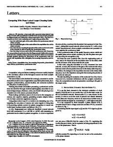
belongs to the large class of npcomplete (nondeterministic polynomial time complete) problems, just a~ the traveling salesperson problem (TSP). The complexity of job-shop scheduling is characteristics of many other real-life situations, albeit in a different context: the scheduling of classes to classrooms, courses to professors, hospital patients to beds, and so forth. In a job-shop problem, each operation is described by a triplet (i,j,k),i.e., operation i of job i is to be executed on machine k. Assuming there are m machines, then each job has exactly m operations with exactly one operation on each machine. If there are n jobs, then each machine must perform n operations. The number of possible scquences is therefore n! for each machine. If the sequences on each machine are independent, there are (n !)" schedules. However, since each job consists of several operations with a linear precedence structure, some these schedules are invalid solutions. An example &job bmachine job-shop problem is shown in Table I. Table l(a) shows the machine assignment for each operation, while Table l(b) lists the corresponding processing time. Figure 1 shows a set of dependency trees describing the operation precedence relationships for the 4-job bmachine problem. A feasible schedule is one where all operations of each job can be placed on one time axis in precedence order and without overlap. One of the simplest and most widely used model for representing jobshop schedule relationships is the Gantt chart. The Gantt chart is a graph of resource allocation over time. Figure 2(a) shows a Gantt chart for a job-shop schedule described in Table 1. Each job-operation-machine triplet is represented by a block; the length of block is equal to the (i,j,k) processing time, i.e., tijk. In principle, there are infinite number of feasible schedules for a given job-shop problem because an arbitrary amount of idle time can be inserted at any machine between pairs of operations. Superfluous idle time exists in a schedule if some operation can be processed earlier in time without altering the operation sequences on any machine. An adjustment called local lejt-shift can be made by moving an operation block to the left on the Gantt chart while preserving the operation sequence. The set of all schedules in which no more local leftshift can be made is called the set of aemiactivc schedules and they do not contain any superfluous idle time. Figure 2(a) shows an example semiactive schedule. In a semiactive schedule, the start time of a particular operation is constrained either by the processing of a different job on the same machine or by the processing of the directly preceding operation on a different machine. As observed in Figure 2(a), there is room for improvements. For instance, operation (3,1,1) can be started at time 0 without delaying any other operation. On the Gantt chart, shifting operation (3,1,1) to the left without delaying any other operation is called a global kft-shift. The set of all schedules in- which no more global leftrshifts can be made is called the sct of active schedules. Figure 2(b) shows an active s i e d u l e . In a nondelay schedule, no machine is kept idle at a time when it could begin processing some operation. In Figure 2(b), note that machine 3 remains idle at time i when it could start on either operation (4,2,3) or (3,2,3). If the job order on machine 3 is changed to 2-3-41, the result would be a nondelay schedule, Figure 2(c). All nondelay schedules are subsets of active schedules. Nondelay schedules can usually be expected to provide a very good solution, although there is no guarantee that a nondelay schedule is the optimum solution. A job-shop problem is completely solved if the starting times of all jobs are determined, and the precedence relationships between the operations are not violated. In general, the optimality criteria for machine scheduling can be classified into various groups. These measures of performance include criteria based on completion-dates (the time at which the last operation of job is completed), flow-times (the amount of time the job spends in the shop), and makespan. Mean flowtime is defined as the average flowtime of a job in the processing sequence. It is computed by summing the completion times on the last machine for each of n jobs and dividing the sum by n. Makespan is the total elapsed time required to process all of a given set of jobs. In many cases, previous researchers have used minimization of makespan as the objective function. 2.1. Deterministic and Heuristic Approaches
As discussed earlier, the number of feasible solutions for sequencing n jobs on m machines for a general job-shop problem is (n!)". By enumerating all possible sequences of jobs (i.e., exhaustive search), optimal solutions are guaranteed. However, for large problems, this is a prohibitively expensive method based on the huge computational time involved. Current procedures for solving job-shop scheduling problems' can be classified into three main categories: deterministic approaches such as branch and bound search technique, heuristic procedures such as
11-276
priority dispatching rules, sampling procedures, probabilistic dispatching procedures, and integer linear programming. Branch and bound approach is a tree-structured procedure for finding an optimal solution. In this approach, the nodes in the tree correspond to partial schedules. As the number of jobs, n, increases, the number of branches grows exponentially by a factor of 2". The effectiveness of branch and bound approach depends on whether good lower bounds can be computed for partial schedules, as studied by Brooks and WhiteD, and Greenbere. For large problems, computational requirements make the branch and bound approach prohibitively expensive to find the optimal solution from the tree of semiactive schedules. This technique is limited to solving relatively small-sized problems. The branch-and-bound algorithm with backtracking guarantees an optimum solution. This technique becomes a heuristic approach when backtracking is not employed. A number of heuristic search techniques have been developed for generating jobshop schedules with optimal solutions. For example, swapping jobs on a machine without violating the precedence order of processing could result in an optimum solution. Since jobshop problems are np-complete, it is apparent that an optimum solution to a large scheduling problem is difficult to find. In most cases, what is truly desired is a very g o o d solution. Heuristic methods produce suboptimal solutions, although they do not guarantee the finding of an optimum solution. Experiments by Jeremiah et. a l l 0 have demonstrated that schedule generation based on priority dispatching rules is a practical method of obtaining suboptimal solutions to jobshop problems. Integer linear programming is a mathematical approach to solving sequencing problems. In this approach, a job-shop problem is formulated as a set of linear constraint equations. Often, optimal solutions are guaranteed in both small and large problems. However, as the size of problem increases, there is a polynomial growth in the number of constraints and variables. Foo and Takefujil presented a mixed integer linear programming (MILP) network for solving jobshop problems. This MEP approach involves an iterative linear optimization technique with integer adjustments to solve a set of integer linear equations. Depending on the requirements and constraints (e.g., computation costs, and problem size), an appropriate technique for solving jobshop problems can be selected from the classes of approaches. In general, a branch and bound approach is practical for small problems, while for large problems, stochastic and mathematical approaches are suggested. The complete report of our stochastic approach to solving jobshop problems is organized into 2 papers. This first paper (Part 1) provides an informal definition of jobshop scheduling, and then formulates the problem based on Hopfield neural network model. The second paper (Part 2) details the architecture of a stochastic neural computation network for solving job-shop problems. The simulated annealing algorithm is also presented, and the software simulation results analyzed. 3. Hopfield Neural Network Model
Hopfield and Tank2 introduced a deterministic neural network model with a symmetrically interconnected network. Figure 3 shows the basic architecture of a Hopfield neural circuit. Each biological neurons is simulated by an operational amplifier that has a sigmoid input/output function defined as:
V;
1 2
= g ( u ; ) = - (1
+ tanh Xu;)
(3.1)
where U ; and are input and output voltages, respectively, of the i-th operational amplifier, and X is the gain factor. If X >> 1 (i.e., amplifier in high-gain mode), then the relation (3.1) becomes approximately a step function. Synapses are represented as resistive connections between neurons. The strength of each synapse is determined by conductance G;j which connects one of the two outputs of 5 t h amplifier to the input of A h amplifier. This interconnection is made possible with a resistor Rij, where Rij = 1/Gij. An externally supplied input. current I; for each neuron is used to set the level of excitability of the network through constant biases. The input bias currents can be used to shift the input-output relation along the U ; ayis, and to turn on specific neurons ("clamping") by introducing a constant bias voltage. It can be easily shown that the equation of motion describing the time evolution of the analog circuit is: (3.2)
11-277
where time constant ri of the i-th operational amplifier is determined by ri = R,-Ci, and Ci is the total input capacitance. The total input resistance Ri is the parallel combination of all input resistances given by:
where pi is the input resistance at the i-th operational amplifier. In order to have the same time constant 7 for all neurons, it is desired to have the total resistance R matched. Hopfield' has shown that the equations of motion for a network with symmetric connections (Gij = Gji) alwvays lead to a convergence of stable states, i.e., the outputs of all neurons remain constant. Furthermore, when the amplifiers are in a high-gain mode, the stable states of a network comprising Nneurons are the local minima of the energy
E
=
- 1/'L
N N
Gij vi Vj -
i-1 j-1
N
vih.
(3.4)
i-1
The state space over which the circuit operates is the interior of the N-dimensional hypercube defined by V,. = 0 or 1. By choosing appropriate values for the synapse strengths, input currenb, and gains of amplifiers, the system can be programmed to find optimum solutions to a wide variety of optimization and constraint satisfaction problems. 4. Problem Formulation
Solving an optimization problem with constraints satisfaction requires selecting an appropriate representation of the problem, and choosing the appropriate weights for the connections and input biases. We chose the Hopfield neural network model to represent the jobshop problem because of its simplicity and proven success in providing good solutions to many optimization problems. In our approach, the familiar matrix representation of neurons for solving the TSP is wed. This Hopfield TSP-type network is organized as a matrix of neurons with (mn + 1) rows and mn columns, where n and m are the number of jobs and the number of machines, respectively. Figure 4 shows the organization of neurons for solving a &job bmachine problem described in Table 1. As shown in Figure 4, each operation ( i , j , k ) of the jobshop problem is a variable on both axes. Each entry in the matrix represents a hypothesis that node ( i , j , k )is dependent on node (p,q,r).
A set of these hypotheses is used to construct a cost function tree. With reference to Figure 4, if amplifier
816
is turned on, then the hypothesis operation (1,2,2) is dependent on operation ( l , l , l )
is true. A column of null's (0's) is inserted to provide the hypothesis that an operation (i,j,k) does not depend on any other operation, i.e., it can start at time 0. Based on this scheme, the total number of neurons needed to represent the jobshop problem is N = mn(mn + I). The corresponding weight matrix G consists of [mn (mn + 1))' interconnections. There are three basic constraints to be encoded in the neural network. These conditions are: (1) no more than m number of jobs are allowed to start at time 0, (2) self-dependency on each operation is not allowed, and (3) precedence relationships between operations must be obeyed.
If there are n jobs and m machines available, then at most m jobs can start independently at time 0. Constraint of type (1) arises when n > m. In this situation, it may be necessary to randomly choose m out of n unique jobs to start at time 0. Hence a mechanism to randomly trigger m neurons out of n choices is required.
11-278
Constraint of type (?) is necessary to avoid self-recurring dependency paths. This condition is enforced by placing strong inhibitions (negative bias) at appropriate neurons such these neurons will not trigger. Constraint (3) is important such that the precedence order of processing each operation is not violated. For example, the hypothesis that operation (i, 2,k) is dependent on operation (i, 1 , p ) should never be true. Again, strong inhihitory (negative) currents are applied at appropriate neurons to enforce the operation precedence relationships. Figure 5 shows a neuron matrix encoded with constraints for the Cjob bmachine problem through assigning appropriate input bias currents ~ ~ o w , c o , . Strong inhibitions are represented by a negative current of an arbitrary value (e.g., - 0.10).For example, since operation ( I , I , I ) is not allowed to depend on are assigned the value - 0.10. Strong itself and operations (1,?,2) and (1,3,3), bias currents 11,3and inhibitions are also placed a t 12,1and 13,1since operations (1,2,2) and (1,3,3) are not allowed to start at time 0. For problems requiring associative recall such as pattern recognition, learning rules are used to establish the connection weight (or conductance) Gij between node i and j. For npcomplete problems characterized by combinatorial complexity, the weights are usually established in a priori manner. Since each operation is only allowed to depend on one other operation, only one neuron is expected to turn on a t any row. Another requirement is that exactly mn number of neurons must "fire". Hence the row and global inhibitions. However, due to constraint (3), there is no column inhibitions, but rather m number of neurons must "fire". Based on our problem formulation, the global energy function which contains the constraints of a jobshop problem is defined as:
r
i
where V i and I, axe the output voltage and input bias current of neuron in position ( z , i ) of matrix, respectively. Constant A is a connection coefficient corresponding to the row inhibition, while B is the global inhibition term to enforce the requirement that exactly mn neurons are in the "firing" state. Both coefficients are arbitrary positive constants since they are problem dependent. The first term of equation (4.1) is zero if and only if each row in the matrix of neurons do not contain more than one "firing" neuron (i.e., turned on), the rest of the neurons in that particular row being turned ofl The second term is zero if and only if there are z neurons being turned on in the whole matrix of neurons. Equating the terms in equation (3.4) and equation (4.1), each entry in the conductance G matrix is the sum of appropriate row and global inhibitions, i.e., G ~ , , ,= j - A &(I - Sij) "inhibitory connections within each row" -B "global inhibition"
si.
=1
if i = j, and is 0 otherwise.
(4.2)
where each entry Gn;vj denotes the connection of neuron in row z and column i of the connection array with the neuron in row y and column j. From equations (3.3) and (4.?), the linear differential equation of motion describing the behavior of the Hopfield network with Nneurons is
where T is the time constant of circuit, and U, is the input voltage to neuron. For simplicity, 7 can be set to 1 . The solution is obtained when the network is stable, and each neuron is either o n ( V 2 .5V) or of( V < .5V). The construction of the cost function trees from the matrix representation is rather straightforward as explained earlier. The cost of path connecting operation ( i , j . k ) to operation ( p , q , r ) is the value of timing information Iijk. A collection of the dependency paths interpreted from the matrix representation will form t n number of trees. The nodes of the trees represent operations, and the links represent the interdependency between jobs. Each top node (root) represents a null operation with zero processing time. The cost attached to each link is a function of the processing time of a particular operation. The total completion times of all jobs
11-279
can be determined by traversing each leaf node leading to the root, node of a tree. T h r starting time za of operation ( i , j , k ) is the sum of the processing times added from the paths iinecting the node to its root minus the cost of the first immediate path. Figure 6 shows an example jobshop problem and its transformation process from the matrix output (solution) to the Gantt chart. The sequel to this paper (Part 2) will discuss the architecture of the neural computation algorithm, and provide a summary of the simulation results. 5. Conclusion
We have introduced a neural network computation scheme for solving job-shop problems. Based on a set of constraints programmed into the neural network, solutions to job-shop problems can be found. A jobshop schedule is determined by evaluating the cost function trees encoded on a neuron matrix of stable states. Since job-shop problems are npcomplete, it is apparent that an optimum solution to a larcy problem is difficult to find. However, in most cases, what is truly desired is a very good solution. Tliis stochastic approach produce near-optimal solutions, although it does not guarantee the finding of an optimum solution. The drawback of our approach is that N = m n ( m n + 1) number of neurons and A@ interconnrctions are needed to solve an n-job m-machine problem. Obviously, for large size problems, this approach is not very feasible. Other alternatives include an integer linear programming network approach presented by Foo and Takefuji'l, which show significant savings in hardware requirement and computations. 6. References
[I] J.J. Hopfield and D.W. Tank, "Computing with Neural Circuits: A Model," Science Vol. 233, Aug. 1986. [2] J.J. Hopfield and D.W. Tank, "Neural Computation of Decisions in Optimization Problems," Biological Cybernetics, Vol. 55, pp. 141-152, 1985. [3] D.W. Tank and J.J. Hopfield, "Simple Neural Optimization Networks: An A/D Converter, Signal Decision Circuit and Linear Programming Circuit," E E E Trans. on Circuits and Systems, Vol. CAS33, NO. 5, pp. 533-541, 198G. [4] J. J. Hopfield, "Neurons with graded response have collective computational properties like those of t w e state neurons," Proc. Natl. A c a d . Sei. USA, Vol. 81, 1984, pp. 30883092. [5] G A . Tagliarini and E.W. Page, "Solving Constraint Satisfaction Problems with Neural Networks", IEEE 1 s t Int. Conf. on Neural Networks, San Diego, CA, June 1987. [6] S. Kirkpatrick, C.D. Gelatt Jr., and M.P. Vecchi, "Optimization by Simulated Annealing," Science, Vol. 220, No. 4598, May 1983. [7] K.R. Baker, "Introduction to Sequencing and Scheduling," John Wiley & Sons, 1974. [8] H. Greenberg, "A Branch and Bound Solution to the General Scheduling Problem," Operations Research, Vol. 16, No. 2, March 19G8. 191 G.H. Brooks, and C.R. White, "An Algorithm for Finding Optimal and Near-optimal Solutions to the Production Scheduling Problem," Journal of Industrial Engineering, Vol. 16, No. 1, January 1985. [lo] B. Jeremiah, A. Lalchandani, L. Schrage, "Heuristic Rules toward Optimal Scheduling," Research Report, Dept. of Industrial Engineering, Cornel1 University, 1984. 1111 M. 0. Poliac, E. B. Lee, J. R. Slagle, M. R. Wick, "A Crew Scheduling Problem," IEEE 1st Int. Conf. on Neural Networks, San Diego, CA, June 1987. [12] Y. P . S. Foo and Y. Takefuji, "Neural Optimization of JobShop Scheduling: A Mixed Integer Linear Programming (MILP) Network", submitted to IEEE Transactions on Computers.
11-280
Machine Assignment
1
4
I
2
3
i J
Figure 1. Operation precedence relationships for +job $machine problem.
Processing time
11 Ii
,r
lki
M3
M1
M2
M3
4.1.2
2.1.3
M2
1.2.2
4.1.2
4.3.1
2.3.2
3.3.2
1 7
1.1,l
4.2.3
.2.1
1.1,:I
0
M1
3.2.3
2.1.3
13 15
26
2.2.1
1.2.2
33
4.3.1
2.3.2
3.3.2
Figure 2. Gantt charts of (a) semiactive, (b) active, and (c) . nondelay schedules.
1111
=5
tu2
=8
tpl = 5
tla = 6 (1)
0
212
111
122 212
0
221
0
0
0
0
(b)
v1
"2
vl
v2
Figure 3. Architecture of Hopfield neural circuit. Each neuron is represented by a set of non-inverting and inverting operational amplifiers The output of a neuron can be connected to the input of any other neuron. Dark squares at intersections represent resistive connections, G,l's. Connections between inverted outputs and inputs to the operational amplifiers represent inhibitory synapses.
8 221
ml
w
d
1.1.1
1.1.1
g1
g2
1.2.2
gum42
%"U3
1.23
0 0 0
0.0
gX-l)
Figure 6. An example 2-job &machine problem showing the (a)timing information, (b) matrix representation of solution, (c) cost function trees, and (d) Gantt chart.
1.3.3 0 0 0
0 0 0
0 0 0
0 0 0
4.2.3 4.3.1
'bd2 g(d%l
gN
Figure 4. Organization of neurons based on mn-by-mn(mn+l) matrix representation. 0.0 -0.1 -0.1 -0.1 -0.1
-0.1 0.0
-0.1 -0.1
0.0 -0.1
-0.1 0.0
-0.1 -0.1
0.0
0.0 0.0 0.0 0.0 0.0 0.0 0.0 0.0 0.0 0.0 0.0 0.0 0.0 0.0 0.0 0.0 0.0 0.0 0.0 0.0 0.0 0.0 -0.1 -0.1 0.0 0.0 0.0 0.0 0.0 -0.1 -0.1 0.0 0.0 0.0 0.0 0.0 0.0 -0.1 0.0 0.0 0.0 0.0 0.0 0.0 0.0 -0.1 -0.1 -0.1 0.0 0.0 0.0 0.0 0.0 -0.1 -0.1 0.0 0.0 0.0 0.0 0.0 0.0 -0.1 0.0 0.0 0.0 0.0 0.0 0.0 0.0 -0.1 -0.1 0.0 0.0 0.0 0.0 0.0 0.0 -0.1 0.0 0.0 0.0 0.0 0.0 0.0 0.0
-0.1 -0.1 0.0 0.0 0.0 -0.1 0.0 0.0 0.0 0.0 -0.1 0.0 0.0 0.0 0.0 0.0 0.0 0.0 0.0 0.0 0.0 0.0 0.0 0.0 0.0 0.0 0.0 0.0 0.0 0.0 0.0 0.0 0.0 0.0 0.0 0.0 0.0 0.0 0.0 0.0 0.0 0.0 0.0
l 2 2 l l
g-1
.L4
0 0 0
111
4.3.1
k
2
. I I
0.0 0.0 0.0 0.0 0.0 0.0 0.0 0.0
0.0 -0.1 -0.1 -0.1
Figure 5. Matrix representation of bias currents to neural network.
11-282