Stochastic Solution for Uncertainty Propagation in Nonlinear Shallow-Water Equations Liang Ge1; Kwok Fai Cheung2; and Marcelo H. Kobayashi3 Abstract: This paper presents a stochastic approach to describe input uncertainties and their propagation through the nonlinear shallowwater equations. The formulation builds on a finite-volume model with a Godunov-type scheme for its shock capturing capabilities. Orthogonal polynomials from the Askey scheme provide expansion of the variables in terms of a finite number of modes from which the mean and higher-order moments of the distribution can be derived. The orthogonal property of the polynomials allows the use of a Galerkin projection to derive separate equations for the individual modes. Implementation of the polynomial chaos expansion and its nonintrusive counterpart determines the modal contributions from the resulting system of equations. Examples of long-wave transformation over a submerged hump illustrate the stochastic approach with uncertainties represented by Gaussian distribution. Additional results demonstrate the applicability of the approach with other distributions as well. The stochastic solution agrees well with the results from the Monte Carlo method, but at a small fraction of its computing cost. DOI: 10.1061/共ASCE兲0733-9429共2008兲134:12共1732兲 CE Database subject headings: Long waves; Monte Carlo method; Polynomials; Shallow water; Stochastic models; Wave propagation.
Introduction The nonlinear shallow-water equations have a wide variety of applications in modeling flood hazards associated with openchannel and dam-break flows, tides and storm surge, and tsunamis. Such events may develop large amplitudes and inundate lowlying areas causing casualties and property damage. The input environmental conditions of these events involve a certain degree of uncertainty, and in most cases follow some form of statistical distributions. Apart from being able to model these extreme flood events, the capability of accounting for the variability of the input parameters is important to flood hazard assessments. Recent advances in shallow-water models based on Godunovtype schemes provide accurate descriptions of extreme flood events involving discontinuous flows. The finite-volume method has the advantage of solving the integral form of the nonlinear shallow-water equations as a fully conservative scheme. Dodd 共1998兲 and Hu et al. 共2000兲, respectively, used a Roe-type and a Harten–Lax–van Leer 共HLL兲 approximate Riemann solver in onedimensional long-wave runup and overtopping models. Hubbard and Dodd 共2002兲, Bradford and Sanders 共2002兲, and George 共2008兲 implemented long-wave propagation and runup models in 1 Graduate Research Assistant, Dept. of Ocean and Resources Engineering, Univ. of Hawaii, Honolulu, Hawaii 96822. 2 Professor, Dept. of Ocean and Resources Engineering, Univ. of Hawaii, Honolulu, Hawaii 96822 共corresponding author兲. E-mail:
[email protected] 3 Associate Professor, Dept. of Mechanical Engineering, Univ. of Hawaii, Honolulu, Hawaii 96822. Note. Discussion open until May 1, 2009. Separate discussions must be submitted for individual papers. The manuscript for this paper was submitted for review and possible publication on August 24, 2007; approved on June 10, 2008. This paper is part of the Journal of Hydraulic Engineering, Vol. 134, No. 12, December 1, 2008. ©ASCE, ISSN 07339429/2008/12-1732–1743/$25.00.
two dimensions using approximate Riemann solvers, while Brocchini et al. 共2001兲, Wei et al. 共2006兲, and Pan et al. 共2007兲 used the exact 共iterative兲 Riemann solver instead. The finite-volume method also has applications in modeling open-channel and dambreak flows and provides accurate results 共e.g., Zhou et al. 2001; Wu and Cheung 2008兲. Most of the recent research efforts in shallow-water models focus on the numerical schemes with deterministic input conditions and precisely defined topography. With the models becoming mature and the computational capability improving, it is timely to seek a method that can handle propagation of uncertainties through the modeling process to provide a risk-based approach for flood hazard assessments. The probabilistic approach, which simulates random events from statistical distributions or recorded data, is by far the most common 共e.g., Scheffner et al. 1996; Geist and Parsons 2006兲. The Monte Carlo simulation techniques, however, have low convergence rates and become computationally prohibitive for large computational problems. A more efficient approach proposed by Ghanem and Spanos 共1991兲 in the context of solid mechanics uses spectral representations of input uncertainties and their propagation through the modeling process. The method, which is based on the theory of Wiener 共1938兲 on homogeneous chaos, provides a high-order representation of the uncertainty and has the promise of a substantial speed up compared to the Monte Carlo approach. Polynomial chaos, which is a generalization of the homogeneous chaos, has recently received attention in computational fluid dynamics. Debusschere et al. 共2004兲 provided a comprehensive review of the method and discussed its numerical challenges. The original polynomial chaos expansion of Wiener 共1938兲 employs the Hermite basis to represent Gaussian processes. Maitre et al. 共2001兲 implemented this approach to model propagation of input Gaussian uncertainties through Navier–Stokes simulations. Xiu and Karniadakis 共2003兲 extended the method to most commonly known statistical distributions using the 13 hypergeometric
1732 / JOURNAL OF HYDRAULIC ENGINEERING © ASCE / DECEMBER 2008
Downloaded 17 Nov 2008 to 128.171.57.189. Redistribution subject to ASCE license or copyright; see http://pubs.asce.org/copyright
orthogonal polynomials in the Askey scheme and provided encouraging results for non-Gaussian processes in viscous flows. The polynomial chaos expansion has also provided stochastic solutions to other flow problems involving the diffusion equation by Xiu and Karniadakis 共2002兲 and the Euler equations by Perez and Walters 共2005兲. In this paper, we examine the implementation of the polynomial chaos method to describe input uncertainties and their propagation through the nonlinear shallow-water equations. This represents an important first step in developing an efficient approach to incorporate long- and short-term variability of environmental forcing in flood hazard modeling. The following section provides a summary of the finite-volume formulation of the nonlinear shallow-water equations and the Godunov-type scheme with a Roe-type approximate Riemann solver. This is followed by the formulation of the stochastic shallow-water equations using the polynomial chaos expansion. The use of an approximate Riemann solver allows the solution to be obtained by the conventional as well as the recently proposed nonintrusive polynomial chaos scheme of Hosder et al. 共2006兲. Two one-dimensional numerical examples involving long-wave propagation over a hump illustrate the implementation of the two schemes and the propagation of uncertainties. The results are compared with Monte Carlo simulations to provide a general indication on the effectiveness and efficiency of the two polynomial chaos schemes.
⌬t ˜ − ˆ k+1 = Qk+1/2 − ⌬t 关A+⌬Q Q 关Fi+1/2 − ˜Fi−1/2兴 i−1/2 − A ⌬Qi+1/2兴 − i i ⌬x ⌬x 共8兲 where A = F / Q denotes the Jacobian matrix of the flux; ⌬Q represents the jump discontinuities; and ˜Fi⫾1/2 provides secondorder flux corrections. In Eq. 共8兲, the term A+⌬Qi−1/2 measures the flux fluctuation due to all right-propagating waves from the interface at xi−1/2; and A−⌬Qi+1/2 measures the net effect of all left-propagating waves from xi+1/2. Since the Roe-type approximate Riemann solution for the one-dimensional shallow-water equations consists of two waves, the flux fluctuation at the cell interface 共i − 1 / 2兲 is given by A ⌬Qi−1/2 =
共1兲
冋
H Hu
Hu F= 2 Hu + gH2/2
共2兲
册
冤 冥
0 h S= gH x
共3兲
⌬t k S 2 i
m m ,0兲Wi−1/2 兺 max共s¯i−1/2
共9兲
m=1
m m = eigenvalues of A; and Wi−1/2 = mth wave of the Riewhere ¯si−1/2 mann solution. The eigenvalues can be defined as
冑
1 ¯ ¯si−1/2 = ¯ui−1/2 − gH i−1/2
冑
2 ¯ and ¯si−1/2 = ¯ui−1/2 + gH i−1/2
共10兲 ¯ in which ¯ui−1/2 and H i−1/2 indicate averages of the flow velocity and depth given by Roe 共1981兲 as ¯ui−1/2 =
ui−1冑gHi−1 + ui冑gHi
冑gHi−1 + 冑gHi
and
Hi + Hi−1 ¯ H 共11兲 i−1/2 = 2
m m m m ¯ri−1/2 = ¯␣i−1/2 with ¯␣i−1/2 from the vector The mth wave Wi−1/2 −1 ¯ i−1/2 = R ⌬Qi−1/2, where R denotes the matrix of eigenvectors ␣ 1 ¯ri−1/2 =
冋 册 1
1 ¯si−1/2
,
2 ¯ri−1/2 =
冋 册 1
2 ¯si−1/2
共12兲
The second-order flux correction term is given by M
共4兲
where h⫽water depth; g = gravitational acceleration; H⫽flow depth; and u=flow velocity. The nonlinear shallow-water equations are hyperbolic and can admit discontinuous solutions. A Godunov-type scheme based on the solution of a local Riemann problem provides an effective approach to capture the pertinent flow characteristics. With Qki denoting the average value of the solution at grid cell i and time step k, the fractional-step method update the solution as = Qki + Qk+1/2 i
共7兲
2
where t denotes time and x the horizontal axis. The vector of conserved variables Q, the flux vector F, and the source vector S are given, respectively, by
冋 册
ˆ k+1 + ⌬t Sˆ k+1 =Q Qk+1 i i 2 i
+
The governing equations for long-wave propagation can be derived in many methods via depth integration under the assumption that the flow is hydrostatic or the vertical velocity component is negligible. The resulting nonlinear shallow-water equations, which include a continuity equation and a momentum equation, can be written in the conservative form as
Q=
共6兲
where 共ˆ 兲 indicates an intermediate solution at a given time step; and ⌬x and ⌬t represent the cell and time-step sizes, respectively. Instead of directly calculating the flux Fi⫾1/2 in Eq. 共6兲, one efficient way is to calculate the flux fluctuations through the approximate Roe-type Riemann solver as
Nonlinear Shallow-Water Equations
Q F + =S t x
ˆ k+1 = Qk+1/2 − ⌬t 关Fk+1/2 − Fk+1/2兴 Q i i i−1/2 ⌬x i+1/2
共5兲
冉
冊
1 ⌬t m m ˜F ˜m ¯i−1/2 ¯ 兩s 兩s 兩 1− 兩 W i−1/2 = i−1/2 2 m=1 ⌬x i−1/2
兺
共13兲
˜ m denotes the limited version of the mth wave given where W i−1/2 by LeVeque 共1998兲. A similar set of expressions can be derived at the interface 共i + 1 / 2兲 and is not repeated here.
Polynomial Chaos Method The polynomial chaos expansion introduces a new dimension to the physical problem to account for the uncertainty. The variables in the governing differential equations can be represented by a series of orthogonal polynomials, which for computational pur-
JOURNAL OF HYDRAULIC ENGINEERING © ASCE / DECEMBER 2008 / 1733
Downloaded 17 Nov 2008 to 128.171.57.189. Redistribution subject to ASCE license or copyright; see http://pubs.asce.org/copyright
poses, is truncated after a finite number of modes. In the present study, the vector of conserved variables in the nonlinear shallowwater equations is expanded to include a random variable as P
Q共x,t,兲 =
Qn共x,t兲⌽n共兲 兺 n=0
共14兲
where n denotes the mode; P = order of the expansion; Qn共x , t兲 = polynomial coefficient; and ⌽n共兲 = polynomial chaos basis representing the uncertainty in random space. This expression separates the evolution of the stochastic variable Q共x , t , 兲 into a deterministic part, given by the coefficient Qn共x , t兲, and a random component modeled by the polynomial chaos basis ⌽n共兲. Xiu and Karniadakis 共2003兲 showed that there are specific polynomials in the Askey scheme for the best convergence of 13 common statistical distributions in the polynomial chaos expansion. As an illustration, the present study considers the propagation of input uncertainties described by Gaussian and beta distributions. The Hermite polynomial provides the best convergence rate for Gaussian distribution. The multidimensional Hermite polynomial of order n is expressed in terms of Gaussian variables =共i1 , . . . , in兲 with zero mean and unit variance as
⌽n共;␣,兲 =
冦
n T e−1/2 i1 . . . in
⌽n =
冦
1
for n = 0 for n = 1 for n = 2 2 − 1 3 for n = 3 − 3 4 − 62 + 3 for n = 4
冧
⌽n共;␣,兲 =
共− 1兲n dn −␣ − 共1 − 兲 共1 + 兲 关共1 − 兲n+␣共1 + 兲n+兴 dn 2nn! 共17兲
where −1 ⬍ ⬍ 1; and ␣ and  ⬎ −1. As an illustration, the zeroth and the first two orders of the Jacobi polynomial are
冧
共18兲
⌫共␣ + 1兲⌫共 + 1兲 ⌫共␣ +  + 2兲
共22兲
for n = 0
共19兲
where W共兲 = weight function. For the Hermite polynomial, Gaussian distribution provides the weight function
W共兲 =
B共␣ + 1, + 1兲 =
The orthogonal property of the polynomial chaos basis gives rise to 具⌽i⌽ j典 = 具⌽2i 典␦ij
⌽i共兲⌽ j共兲W共兲d
1
冑2 e
−2/2
共20兲
The weight function for beta distribution is derived from the Jacobi polynomial chaos basis as 共1 − 兲␣共1 + 兲 W共兲 = B共␣ + 1, + 1兲 in which the beta function is given by
共16兲
which may be readily used in Eq. 共14兲 to represent Gaussian uncertainties. For beta distribution, the one-dimensional nth-order Jacobi polynomial is defined as
␣− 2+␣+ for n = 1 − 2 2 1 1 1 共3 + ␣ + 兲共4 + ␣ + 兲共 − 1兲2 + 共2 + ␣兲共3 + ␣ + 兲共 − 1兲 + 共1 + ␣兲共2 + ␣兲 for n = 2 8 2 2
冕
共15兲
where the subscript i relates to the dimension of the polynomial. For example, the zeroth and the first four orders of the Hermite polynomial in one dimension are
1
There are 11 other hypergeometric orthogonal polynomials for specific statistical distributions. The use of a different polynomial may result in unstable solutions or low convergence rates, requiring more modes to approximate the statistical distribution. The polynomial chaos forms a complete orthogonal basis in the Hilbert space. The ensemble average of the basis functions in the Hilbert space is defined as
具⌽i共兲⌽ j共兲典 =
T
⌽n共兲 = e1/2 共− 1兲n
共23兲
where ␦ij = Kronecker delta. The relation is valid for any of the hypergeometric orthogonal polynomials in the Askey scheme. In the present study, we utilize the conventional and the nonintrusive approaches for the implementation of the polynomial chaos expansion. Both approaches utilize the orthogonal property of the basis functions in Eq. 共23兲 to derive separate equations for the individual modes. The resulting system of equations defines the modal contributions in the stochastic processes. Once the polynomial coefficients are determined, the mth moment of the stochastic solution is given by
m关Q共x,t,兲兴 =
共21兲
冕
⬁
Qm共x,t,兲W共兲d
共24兲
−⬁
The mean solution is simply given by the zeroth-order coefficient Q0共x , t兲 and the variance by
1734 / JOURNAL OF HYDRAULIC ENGINEERING © ASCE / DECEMBER 2008
Downloaded 17 Nov 2008 to 128.171.57.189. Redistribution subject to ASCE license or copyright; see http://pubs.asce.org/copyright
P
var关Q共x,t,兲兴 ⬇
兺 n=1
Q2n共x,t兲具⌽2n共兲典
共25兲
by the polynomial chaos explicitly. These terms, however, can be determined by numerical integration as J
Higher-order statistical parameters such as the skewness and kurtosis of the stochastic solution likewise can be derived from Eq. 共24兲.
具A ⌬Qi−1/2⌽l典 ⬇ +
冉
p
p jA 兺 Qn⌽n,j 兺 j=1 n=0 +
冊
冉兺 冊 冊冏 兺 兺 冏 冉兺 冉 冏 冉 兺 冊冏冊 冉 兺 冊 p
⫻ ⌬Qi−1/2
Qn⌽n,j ⌽lW j
共33兲
n=0
Stochastic Shallow-Water Equations
J
The conventional polynomial chaos approach transforms the governing equations to a stochastic form, and time integration of the resulting equations provides the polynomial coefficient Qn共x , t兲. Representing the conserved variables in Eq. 共1兲 by the polynomial chaos expansion from Eq. 共14兲 gives a stochastic form of the nonlinear shallow-water equation as P
F =S Q n⌽ n + t n=0 x
兺
共26兲
The equation can be rearranged in the Godunov-type formulation with the Roe-type approximate Riemann solver as P
p
k Qk+1/2 兺 i,n ⌽n = 兺 Qi,n⌽n + n=0 n=0
⌬t k S 2 i
共27兲
˜ 具F i−1/2⌽l典 ⬇
M
pj
j=1
⫻ 1−
1 ¯sm 2 m=1 i−1/2
p
⌬t
ˆ k+1⌽ = 关A+⌬Qi−1/2 − A−⌬Qi+1/2兴 Q Qk+1/2 n 兺 兺 i,n i,n ⌽n − ⌬x n=0 n=0 − P
⌬t ˜ 关Fi+1/2 − ˜Fi−1/2兴 ⌬x P
ˆ k+1 Qk+1 兺 i,n ⌽n = 兺 Qi,n ⌽n + n=0 n=0
p
n=0
where J = number of collocation points; subscript j = collocation point index; and p j = weight of the Gaussian quadrature in random space. The source terms in Eqs. 共30兲 and 共32兲 account for the variation of the topography in space. The topography may contain errors or uncertainties and may be described similarly by the polynomial chaos expansion as P
S=
ˆ k+1 = Qk+1/2 − Q i,l i,l −
⌬t 具Ski ⌽l典 2具⌽2l 典
共29兲
共30兲
⌬t 兵具A+⌬Qi−1/2⌽l典 − 具A−⌬Qi+1/2⌽l典其 ⌬x具⌽2l 典
⌬t ˜ ˜ 兵具F i+1/2⌽l典 − 具Fi−1/2⌽l典其 ⌬x具⌽2l 典 ˆ k+1 Qk+1 i,l = Qi,l +
⌬t ˆ k+1 具Si ⌽l典 2具⌽2l 典
Qn⌽n,j ⌽lW j
n=0
hn共x兲⌽n共兲 兺 n=0
共35兲
Substituting Eq. 共35兲 into Eq. 共4兲, we have the stochastic form of the source term
where Si, A⫾⌬Qi⫿1/2, and ˜Fi⫾1/2 are calculated from the polynomial chaos expansion in terms of Qn and ⌽n. Projecting Eqs. 共27兲–共29兲 onto an arbitrary basis ⌽l with l = 0 , . . . , P, and invoking the ensemble average from Eq. 共23兲, we derive a set of uncoupled equations with the inner products of polynomial chaos bases as coefficients Qk+1/2 = Qki,l + i,l
˜m W i−1/2
Qn⌽n,j
共34兲
共28兲 ⌬t ˆ k+1 S 2 i
Qn⌽n,j
n=0
p
⌬t m ¯s ⌬x i−1/2
h共x,兲 = p
p
冤
0 P
H m⌽ m g x m=0
兺
冉兺 冊 冥 P
共36兲
h n⌽ n
n=0
where Hm denotes the polynomial coefficient of the flow depth and is given by the vector Q. The ensemble average with the polynomial chaos basis becomes 具Ski ⌽l典 =
冤
0 P
P
g Hk 共hi+1/2,n − hi−1/2,n兲具⌽l⌽m⌽n典 ⌬x m=0 n=0 i,m
兺兺
冥
共37兲
With the boundary condition of each mode specified by the corresponding polynomial coefficient, Eqs. 共33兲 and 共34兲 provide the flux terms and Eq. 共37兲 provides the source term for the integration of the 共P + 1兲 modes to the next time step.
Nonintrusive Polynomial Chaos Method 共31兲
共32兲
Eqs. 共30兲–共32兲 represent a set of 共P + 1兲 equations for the solution of the respective modes. The structure of the stochastic shallowwater equations is similar to the deterministic equations 关Eqs. 共5兲–共7兲兴, except for the denominator 具⌽2l 典 and the ensemble averages of the flux and source terms with the polynomial. The ensemble averages of the first- and second-order flux terms in Eq. 共31兲 contain nonpolynomial functions, which cannot be expanded
The so-called nonintrusive polynomial chaos method determines the polynomial coefficients through sampling of the deterministic solution without modifying the governing equations. The core code works as a “black box” with only slight modifications to provide deterministic solutions at predetermined sampling points in random space. This approach is preferred when dealing with lengthy and complex computer codes, which are expensive and time consuming for adaptation. There are several nonintrusive approaches with subtle differences in the sampling scheme. The present study considers the numerical quadrature approach of Hosder et al. 共2006兲, which has provided encouraging results in computational fluid dynamics fields.
JOURNAL OF HYDRAULIC ENGINEERING © ASCE / DECEMBER 2008 / 1735
Downloaded 17 Nov 2008 to 128.171.57.189. Redistribution subject to ASCE license or copyright; see http://pubs.asce.org/copyright
The central idea of the nonintrusive approach is to invert the polynomial chaos expansion in Eq. 共14兲 for the solution of the polynomial coefficients in terms of the deterministic solution. The method utilizes the Galerkin approach to project the stochastic variable Q共x , t , 兲 on to the polynomial chaos basis ⌽l with l =0, ... ,P P
Q共x,t,兲⌽l共兲 =
Qn共x,t兲⌽n共兲⌽l共兲 兺 n=0
共38兲
Taking the ensemble average and invoking the orthogonal properties, Eq. 共38兲 is decomposed into 共1 + P兲 equations for the respective modes 具Q共x,t,兲⌽l共兲典 = Ql共x,t兲具⌽2l 共兲典
共39兲
u共0,t兲 = A冑g/共d + A兲 sech2
冑
3A 共ct − X0兲 4d3
共44兲
in which the celerity is given by c = 冑g共d + A兲
共45兲
where A = wave height; d = water depth 共1 m兲; and X0 = initial position of the input wave 共−35 m兲. The first numerical example deals with the effects of uncertain water depth on wave transformation and the second example examines the evolution in time and space of the uncertainty introduced by the input wave conditions. We perform the stochastic analysis primarily for Gaussian random variables and provide additional results in the second example for beta distribution as a demonstration. The simplicity of the numerical examples allows the stochastic properties of the solution to stand up to a thorough examination.
which leads to 具Q共x,t,兲⌽l共兲典
Ql共x,t兲 =
具⌽2l 共兲典
Uncertainty in Topography 共40兲
Eq. 共40兲 provides an expression to compute the 共1 + P兲 polynomial coefficients from the ensemble average of the random events and polynomial chaos basis. The denominator of Eq. 共40兲 can be precomputed since it is independent of the solution and only depends on the polynomial chaos basis. The ensemble average in the numerator may be determined through numerical integration in stochastic space. A series of random events, Q共x , t , j兲, can be computed at the Gauss– Hermite quadrature points j using the deterministic code. This allows numerical integration of the ensemble average as N
具Q共x,t,兲⌽l共兲典 ⬇
p jQ共x,t, j兲⌽l共 j兲W共 j兲 兺 j=1
共41兲
where N = number of random events used in the integration. This approach uses systematic sampling of random events to determine the polynomial coefficients, which in turn provide the stochastic properties of the events.
Wave propagation over uncertain topography is an interesting topic with many practical applications in open channel flows and coastal hydraulics. Very often, the topography is not precisely defined due to the lack of data or instrumentation errors. In addition, riverbeds and seabeds vary with time and season due to erosion and sedimentation. Some tidal inlets exhibit morphologic processes associated with fluctuation of sediment supplies in a decadal time scale 共e.g., Cheung et al. 2007兲. The capability of incorporating data errors or morphological changes in the prediction of normal or extreme flow conditions is important. In this example, we examine the propagation and transformation of deterministic input wave conditions over a depth profile with Gaussian uncertainties. Both the conventional and nonintrusive polynomial chaos schemes use the Hermite polynomial for the best convergence characteristics. The depth profile defined by Eq. 共42兲 provides a simple test case to illustrate the effect of uncertain topography on free surface flows. The height of the hump is expressed in terms of its mean ¯a and standard deviation a as a共兲 = ¯a + a⌽1共兲
共46兲
The variance of the depth profile is give by 2h = E关h2兴 − E2关h兴
Results and Discussion This study is the first step to examine the feasibility of stochastic shallow-water modeling through the polynomial chaos method. Two simple numerical examples involving long-wave transformation over a hump demonstrate the implementation of the polynomial chaos method and its capability to describe effects of input uncertainties. The examples correspond to a 100-m long and 1-m deep channel with a hump at the center. The depth profile is given by h共x兲 = 1 − a sech2
冑
3a 共x − 50兲 4
共0,t兲 = A sech2
冑
3A 共ct − X0兲 4d3
An approximation of the depth profile by a Taylor series expansion gives 2h ⬇ h2兩¯a +
共43兲
冋冉 冊 h a
2
+h
2h a2
册 冋
2a − h +
¯a
2h 2a a2 2
册
2
共48兲 ¯a
Since a is a small number, we retain terms up to the second order and obtain the variance of the depth profile in terms of ¯a and a as 2h ⬇
共42兲
where a = height of the hump. The input wave conditions are applied at x = 0 and an open boundary condition at x = 100 m. The solitary wave theory provides the input surface elevation and velocity as
共47兲
冏 冏
h 2 2 a ¯a a
共49兲
The Gaussian depth profile is defined by the zeroth mode h0共x兲 computed from ¯a and the first mode h1共x兲 given directly by h共x兲. In the nonintrusive approach, Eq. 共46兲 provides the heights of the hump at the Gauss–Hermite quadrature points for a series of deterministic computations to reconstruct the polynomial coefficients according to Eq. 共40兲. The number of quadrature points is chosen to achieve stability and accuracy with minimum computational costs.
1736 / JOURNAL OF HYDRAULIC ENGINEERING © ASCE / DECEMBER 2008
Downloaded 17 Nov 2008 to 128.171.57.189. Redistribution subject to ASCE license or copyright; see http://pubs.asce.org/copyright
Fig. 1. 共Color兲 Channel profile with ⫾25% error bars
The test conditions correspond to ¯a = 0.4 m, a = 0.08 m, and A = 0.05 m. Fig. 1 plots the mean depth profile with ⫾25% error bars. The profile shows an approximately 10-m-wide hump with an increasing level of uncertainty toward the center. The wave is deterministic at the input boundary and becomes stochastic as it propagates over the uncertain depth profile. Fig. 2 gives the zeroth, first, and second modes of the surface profile along the chan-
Fig. 2. 共Color兲 Polynomial coefficients along the channel. Conventional polynomial chaos approach: black line denotes zeroth mode; blue line denotes first mode; and red line denotes second mode. Nonintrusive polynomial chaos approach: black dots denote zeroth mode; blue dots denote first mode; and red dots denote second mode. 共Note that the first and second modes are exaggerated by two times兲.
nel. The nonintrusive polynomial chaos approach uses 30 quadrature points and provides a converging solution almost identical to that obtained by the conventional expansion, thereby verifying both approaches. The zeroth mode corresponds to the mean surface profile. Since the incident wave is deterministic, the first and second modes are zero before the wave reaches the hump. The uncertainty of the hump profile begins to affect the transformation of the incident waves and generate higher-order modes at t = 25 s. The first and second modes are negative at the narrow wave front, indicating that an increase of the height of the hump would increase the steepness of the wave front. The magnitude of the first and second modes increases as the wave propagates over the hump around t = 30 s. In the limiting case, a bore with a vertical front face develops to mimic the formation of a breaking wave. The polynomial chaos expansion correctly describes the properties of the discontinuous flow. The first and second modes, however, are relatively small at the crest and in the back of the wave. This indicates that changes in the height of the hump only have moderate effects on the transmitted wave height. This result is consistent with that provided by Horritt 共2002兲 using a secondorder perturbation approach. The second mode of the reflection is close to zero, indicating that the reflected wave height follows the Gaussian distribution of the depth profile. Since exact solutions for such a problem are not available, we use the Monte Carlo method to validate the stochastic solution. The results from the Monte Carlo method converge to the exact stochastic solution in a finite number of realizations and provide a baseline for comparison of model accuracy and efficiency. In the Monte Carlo approach, we generate a series of deterministic simulations with the incident wave height A = 0.05 m and randomly selected heights of the hump based on the input statistical parameters ¯a = 0.4 m and a = 0.08 m. This provides a sample of deterministic wave profiles in the channel from which statistics of the output distribution, such as the mean and the variance, can be determined. Fig. 3 compares the mean surface profiles obtained by the Monte Carlo method and the conventional and nonintrusive polynomial chaos approaches. The Monte Carlo solution converges at 1,000 realizations and provides almost identical results as the polynomial chaos method. This confirms the implementation of the polynomial chaos method and its validity in describing propagation of input uncertainties in the nonlinear modeling processes. The probability density function of the stochastic variables can be reconstructed from the polynomial coefficients through a sampling scheme. The required order of expansion for convergence of the probability density function depends on the distribution of the uncertainty and the nonlinearity of the processes. In the present example, the polynomial chaos expansion requires the zeroth and the first four modes to obtain converging results. This requirement is similar to the stochastic quasi-one-dimensional nozzle flow described by Mathelin et al. 共2005兲. The Monte Carlo method, on the other hand, requires 10,000 realizations for convergence of the probability density function. Fig. 4 shows that the polynomial chaos and Monte Carlo methods converge to very similar results. The distribution, in general, is close to Gaussian as indicated by a small second mode in the stochastic solution. There is no uncertainty in the surface profile before the wave reaches the hump. At t = 30 s, most of the wave has propagated over the hump and the uncertainty begins to show effects on the surface wave. Fig. 4共a兲 compares the probability density functions of the surface elevation at x = 35 m, where the reflected wave has its peak, while Fig. 4共b兲 shows the results at the front face of the transmitted wave at x = 65 m. At these two locations, the uncertainty from the depth
JOURNAL OF HYDRAULIC ENGINEERING © ASCE / DECEMBER 2008 / 1737
Downloaded 17 Nov 2008 to 128.171.57.189. Redistribution subject to ASCE license or copyright; see http://pubs.asce.org/copyright
Fig. 3. 共Color兲 Comparison of mean surface profiles: —, conventional polynomial chaos method; -----, nonintrusive polynomial chaos method; and ¯¯, Monte Carlo approach with 1,000 realizations
profile is entrained into the free surface and propagates with the reflected and transmitted waves. Figs. 4共c and d兲 show the respective probability density functions of the reflected and transmitted waves at t = 35 s. The distribution of the reflected wave maintains a small variance, indicating that its amplitude is not very sensitive to changes in the height of the hump. In comparison, the transmitted wave is affected to a greater extent by the uncertainty as indicated by the wider range of surface elevation in the probability distribution function. Uncertainty in Input Wave Conditions The input environmental forcing for modeling of riverine and coastal flood hazards involves a certain degree of uncertainty or error. The capability of determining an error bar for the model prediction based on the input uncertainty is important for quality assurance as well as implementation of the results. Furthermore, occurrence of storms and tsunamis might follow some form of statistical distributions that can be inferred from historical events 共e.g., Scheffner et al. 1996; Geist and Parsons 2006兲. The inverse algorithm of Wei et al. 共2003兲 is capable of providing the mean and standard deviation of far-field tsunami forecasts based on water-level data near the seismic source. The proposed stochastic approach has the potential of providing an efficient description for
Fig. 4. 共Color兲 Probability density function of surface elevation: 共a兲 t = 30 s and x = 35 m; 共b兲 t = 30 s and x = 65 m; 共c兲 t = 35 s and x = 18 m; and 共d兲 t = 35 s and x = 82 m. —, conventional polynomial chaos approach; -----, nonintrusive polynomial chaos approach; and 䊏, Monte Carlo simulation with 10,000 realizations 共note different horizontal scales兲
the propagation of these input statistical distributions through the nonlinear shallow-water equations for flood hazard assessment and warning. In this example, we fix the depth profile along the channel and introduce Gaussian uncertainties into the solution through the input wave conditions. The input wave height is expressed in terms of its mean ¯A and standard deviation A as A共兲 = ¯A + A⌽1共兲
共50兲
Since the water depth h共x兲 is deterministic, the flow depth, H共0 , t兲 = h共0兲 + 共0 , t兲, at the boundary is defined by Eq. 共43兲. The variance of the flow depth is expressed in terms of ¯A and A as H2 ⬇
冏 冏 H A
2 ¯A
2A
共51兲
With a first-order Taylor series expansion, we have the standard deviation of the flux in terms of the mean quantities and H as
1738 / JOURNAL OF HYDRAULIC ENGINEERING © ASCE / DECEMBER 2008
Downloaded 17 Nov 2008 to 128.171.57.189. Redistribution subject to ASCE license or copyright; see http://pubs.asce.org/copyright
Fig. 5. 共Color兲 Input wave profile at boundary: —, mean; and - - - -, first mode
冉
冊
1 ¯ f = ¯c + g H 2 ¯c
共52兲
The mean flow depth and velocity provide the zeroth mode coefficients for the polynomial chaos expansion at the input boundary Q0共0,t兲 =
冋
¯ 共0,t兲 H ¯ 共0,t兲u ¯ 共0,t兲 H
册
共53兲
The standard deviations of the flow depth and flux provide the boundary conditions for the polynomial coefficient of the first mode as Q1共0,t兲 =
冋
H共0,t兲 f 共0,t兲
册
共54兲
This completes the boundary conditions for the polynomial chaos method. In the nonintrusive approach, Eq. 共50兲 provides the wave heights at the Gauss–Hermite quadrature points at which Eqs. 共43兲 and 共44兲 define the boundary conditions for a series of deterministic computations to reconstruct the polynomial coefficients in stochastic space. We demonstrate the stochastic properties of the solution for a = 0.4 m, ¯A = 0.05 m, and A = 0.01 m and employ the Hermite polynomial for optimal convergence. Fig. 5 plots the mean and the first mode of the surface elevation imposed at the boundary. The first mode is negative at the two tails of the wave to account for the profile variation in accordance with the solitary wave theory. The absolute value of the first mode corresponds to the standard deviation of the Gaussian input. The mean surface profile and its standard deviation transform and higher-order modes develop as the wave propagates into the domain. Fig. 6 shows the zeroth, first, and second modes of the stochastic solution along the channel. The nonintrusive approach with 30 quadrature points gives identical results as the conventional polynomial chaos approach. In addition to describing the uncertainty propagation, the stochastic solution provides insights into the wave transformation processes. By t = 15 s, most of the input wave has entered the domain. Both the mean and the first mode of the solution are similar to the input signal. Since the second mode is zero, the wave retains its Gaussian characteristics at this position. As the wave reaches the hump at t = 25 s, both the mean and the first mode become asymmetric and the second mode begins to develop. By t = 35 s, the wave has already passed the hump. The increase in amplitude of the first and second modes results in an overall profile that has a higher and steeper surface and nonGaussian characteristics at the wave front.
Fig. 6. 共Color兲 Polynomial coefficients along the channel. Conventional polynomial chaos approach: black line denotes zeroth mode; blue line denotes first mode; and red line denotes second mode. Nonintrusive polynomial chaos approach: black dots denote zeroth mode; blue dots denote first mode; and red dots denote second mode.
Fig. 7 compares the mean wave profiles from the stochastic solution with the deterministic wave profiles computed from the mean wave height. Error bars covering the 25 and 75 percentiles of the surface profile provide additional information on the stochastic solution. The mean and deterministic wave profiles are identical during the initial propagation as the input Gaussian distribution remains unchanged. When the wave reaches the hump, nonlinear effects associated with the rapid change of water depth become important. A discrepancy between the two solutions begins to develop and the error bars of the stochastic solution widens at the wave front. The deterministic model produces a slightly steeper wave profile. By solving a local Riemann problem, Godunov-type schemes approximate a breaking wave as a bore or hydraulic jump 共e.g., Wei et al. 2006; Wu and Cheung 2008兲. In the stochastic solution, the wave front of the larger waves in the distribution becomes near vertical and a shock condition develops over the hump. This feature places a limit on the wave height increase and skews the distribution. In addition, the stochastic method propagates a family of solutions with different likelihoods of reaching the shock condition, and the shock wave depends on the local conditions of the conservative variables. When compared to the deterministic solution, the expected value of the wave front is diffused as it approaches the shock condition. The Monte Carlo method, which uses deterministic simula-
JOURNAL OF HYDRAULIC ENGINEERING © ASCE / DECEMBER 2008 / 1739
Downloaded 17 Nov 2008 to 128.171.57.189. Redistribution subject to ASCE license or copyright; see http://pubs.asce.org/copyright
Fig. 7. 共Color兲 Comparison of deterministic and stochastic solutions: —, mean surface profile from polynomial chaos method; and -----, deterministic surface profile with mean input wave height. Error bars cover the 25 and 75 percentiles of the surface profile from the polynomial chaos method.
Fig. 8. 共Color兲 Comparison of mean surface profiles: —, conventional polynomial chaos method; -----, nonintrusive polynomial chaos method; and ¯¯, Monte Carlo approach with 1,000 realizations
tions from randomly selected wave heights, provides a baseline for validation of the stochastic solution. Fig. 8 shows identical mean surface profiles obtained from the polynomial chaos method and the Monte Carlo simulation with 1,000 realizations. Fig. 9 also shows good agreement of the probability density functions of the surface elevation from the fourth-order polynomial chaos expansion and the Monte Carlo method with 10,000 realizations. Fig. 9共a兲 shows the results at the mean crest location after the wave propagated 15 s and 14 m from the boundary. The probability density function is close to the input Gaussian distribution inferring that the wave maintains most of its original information at this location. Fig. 9共b兲 shows the probability density function at the crest 48 m from the boundary and 25 s into the calculation. The distribution is no longer perfectly Gaussian, but the change is minor because it is located just behind the wave front, where the second mode, as shown in Fig. 6, is nearly zero. The wave just propagated over the hump at t = 30 s with the crest located at x = 64 m. Fig. 9共c兲 shows the probability density function begins to skew to the right due to breaking of the larger waves in the input Gaussian distribution. The waves continue to break after propagating over the hump, curtailing the maximum wave height and further skewing the distribution as shown in Fig. 9共d兲. Even with
Gaussian input, the subsequent probability distribution through a nonlinear process can become highly skewed and non-Gaussian 共e.g., Mathelin et al. 2005兲. The proposed stochastic analysis is applicable to the 13 commonly used statistical distributions described in Xiu and Karniadakis 共2003兲. As a demonstration, the above calculation was repeated with the input uncertainty defined by beta distribution. The analysis uses the same mean and standard deviation of the wave height at the input boundary for comparison. This gives rise to ␣ = 4,737.65 and  = 5,236.35 in Eq. 共21兲. The input probability density function of the beta distribution is almost identical to that of the Gaussian distribution for these parameters. Both the conventional and nonintrusive polynomial chaos schemes use the Jacobi polynomial for best convergence characteristics. Fig. 10 shows good agreement between the probability density functions obtained from the conventional and nonintrusive polynomial chaos expansions at the fifth order and the Monte Carlo approach with 10,000 realizations. Since we are dealing with the same input uncertainty, the computed probability density functions from the Gaussian and beta random variables, as shown in Figs. 9 and 10, are almost identical. The convergence requirements remain similar as well, thereby verifying the implementation of the proposed stochastic approach for different statistical distributions.
1740 / JOURNAL OF HYDRAULIC ENGINEERING © ASCE / DECEMBER 2008
Downloaded 17 Nov 2008 to 128.171.57.189. Redistribution subject to ASCE license or copyright; see http://pubs.asce.org/copyright
Fig. 9. 共Color兲 Probability density function of surface elevation: 共a兲 t = 15 s and x = 14 m; 共b兲 t = 25 s and x = 48 m; 共c兲 t = 30 s and x = 64 m; and 共d兲 t = 35 s and x = 80 m. —, conventional polynomial chaos approach; -----, nonintrusive polynomial chaos approach; and 䊏, Monte Carlo simulation with 10,000 realizations.
Fig. 10. 共Color兲 Probability density function of surface elevation with Beta input uncertainties: 共a兲 t = 15 s and x = 14 m; 共b兲 t = 25 s and x = 48 m; 共c兲 t = 30 s and x = 64 m; and 共d兲 t = 35 s and x = 80 m. —, conventional polynomial chaos approach; -----, nonintrusive polynomial chaos approach; and 䊏, Monte Carlo simulation with 10,000 realizations.
Computing Time The two numerical examples have shown that both the conventional polynomial chaos method and its nonintrusive counterpart can provide accurate stochastic solutions. For the characteristics of the solution analyzed here, the Monte Carlo method requires 1,000 realizations to match the computed mean surface profiles and as many as 10,000 realizations to capture the skewness of the probability density function. Each realization is a deterministic calculation for given heights of the incident wave and the hump. Since the Monte Carlo method is commonly used in uncertainty analysis, it provides a benchmark for comparison with the two polynomial chaos approaches in this study. The computing time required by the conventional polynomial chaos method to achieve convergence of the probability density function is about 200 times that of a deterministic calculation. This is 50 times more efficient than a Monte Carlo approach. Most of the computing time is spent on the numerical integration of the Reimann solver in Eqs. 共33兲 and 共34兲. Because the solver gives a discontinuous surface profile for a breaking wave, a sufficient number of quadrature points are needed to capture the solution near the discontinuity. The number of quadrature points
is determined by the order of the polynomial chaos in the numerical integration. The computing requirement should be much less in other formulations of the nonlinear shallow-water equations or when wave breaking is not considered. The nonintrusive polynomial chaos method simply comprises a series of deterministic calculations at the Gauss–Hermite quadrature points to cover the distribution in random space. In the present application, the method provides a converging probability density function with about 30 deterministic calculations. These events provide the input for reconstruction of the polynomial coefficients from which statistics of the solution are determined. The computing time for the numerical integration of the ensemble average in Eq. 共41兲 is negligible. The method is about 1,700 times more efficient than the Monte Carlo method in terms of computing time. This illustrates the advantage of a systematic sampling approach in random space versus the use of a much larger sample of randomly selected events. Because of the inherently independent evolution of each mode in the fractional step method used in the finite-volume model, the turnaround time in running both the conventional and nonintru-
JOURNAL OF HYDRAULIC ENGINEERING © ASCE / DECEMBER 2008 / 1741
Downloaded 17 Nov 2008 to 128.171.57.189. Redistribution subject to ASCE license or copyright; see http://pubs.asce.org/copyright
sive polynomial chaos schemes could be sizably reduced using parallel computing. Furthermore, the deterministic calculations for the nonintrusive polynomial chaos method can be performed on separate sets of processors. This allows completion of an uncertainty analysis in a comparable time frame as a deterministic calculation. Thus, the method has the potential of providing uncertainty assessment in real-time flood forecasts associated with storm surge and tsunamis 共e.g., Cheung et al. 2003; Yamazaki et al. 2006; Sánchez and Cheung 2007兲.
Conclusions In this paper, we applied the conventional polynomial chaos method and its nonintrusive counterpart to determine the stochastic solution of the nonlinear shallow-water equations in the conservative form. The method expands the conserved variables as products of polynomial coefficients and orthogonal chaos bases and uses the Galerkin projection to generate a system of equations for the polynomial coefficients. The conventional method requires transformation of the governing equations to the stochastic form and modification of the deterministic code, while the nonintrusive approach determines the polynomial coefficients through sampling of the deterministic code at a number of quadrature points in random space. Numerical examples of long-wave transformation over a submerged hump illustrate the implementation of the polynomial chaos method in nonlinear shallow-water flows. The uncertainty is introduced as the mean and standard deviation of the heights of the input wave and the hump, respectively. The polynomial chaos method can effectively describe the input uncertainties and their propagation and transformation through the modeling processes. Both the conventional and nonintrusive polynomial chaos approaches produce results almost identical to the Monte Carlo method, but at small fractions of its computing cost. The nonintrusive approach, which is highly efficient and does not require modification of the deterministic code, has demonstrated its advantages over the conventional approach in the present application. In addition to uncertainty analysis, the polynomial chaos method is a useful tool for gaining insight into the deterministic solution. The method is capable of resolving stochastic properties across discontinuities in highly nonlinear processes. Analysis of the stochastic solution demonstrates the potential use of the polynomial chaos expansion as a framework to quantify the sensitivity of complex modeling systems to input variables. Although the present study mainly considers Gaussian descriptions of random variables, the same approach is adaptable to most commonly used statistical distributions by selecting the appropriate polynomials from the Askey scheme.
Acknowledgments The research work described in this paper is supported by the Office of Naval Research through Grant No. N00014-02-1-0903. The writers are appreciative of the three anonymous reviewers for their comments and suggestions and to Dr. David L. George for providing the finite-volume source code used in the present study. This is SOEST Contribution 7467.
References Bradford, S. F., and Sanders, B. F. 共2002兲. “Finite-volume model for shallow-water flooding of arbitrary topography.” J. Hydraul. Eng., 128共3兲, 289–298. Brocchini, M., Bernetti, R., Mancinelli, A., and Albertini, G. 共2001兲. “An efficient solver for nearshore flows based on the WAF method.” Coastal Eng., 43共2兲, 105–129. Cheung, K. F., et al. 共2003兲. “Modeling of storm-induced coastal flooding for emergency management.” Ocean Eng., 30共11兲, 1353–1386. Cheung, K. F., Gerritsen, F., and Cleveringa, J. 共2007兲. “Morphodynamics and sand bypassing at Ameland Inlet, The Netherlands.” J. Coastal Res., 23共1兲, 106–118. Debusschere, B. J., Najm, H. N., Pebay, P. P., Knio, O. M., Ghanem, R. G., and Maitre, O. P. L. 共2004兲. “Numerical challenges in the use of polynomial chaos representations for stochastic processes.” SIAM J. Sci. Comput. (USA), 26共2兲, 698–719. Dodd, N. 共1998兲. “Numerical model of wave run-up, overtopping, and regeneration.” J. Waterway, Port, Coastal, Ocean Eng., 124共2兲, 73– 81. Geist, E. L., and Parsons, T. 共2006兲. “Probabilistic analysis of tsunami hazards.” Natural Hazards, 37共3兲, 277–314. George, D. L. 共2008兲. “Augmented Riemann solvers for the shallow water equations over variable topography with steady states and inundation.” J. Comput. Phys., 227共6兲, 3089–3113. Ghanem, R. G., and Spanos, P. 共1991兲. Stochastic finite elements: A spectral approach, Springer, New York. Horritt, M. S. 共2002兲. “Stochastic modelling of 1D shallow water flows over uncertain Topography.” J. Comput. Phys., 180共1兲, 327–338. Hosder, S., Walters, R., and Perez, R. 共2006兲. “A nonintrusive polynomial chaos method for uncertainty propagation in CFD simulations.” Proc., 44th AIAA Aerospace Sciences Meeting and Exhibit, 1–19. Hu, K., Mingham, C. G., and Causon, D. M. 共2000兲. “Numerical simulation of wave overtopping of coastal structures using the nonlinear shallow water equations.” Coastal Eng., 41共4兲, 433–465. Hubbard, M. E., and Dodd, N. 共2002兲. “A 2D numerical model of wave runup and overtopping.” Coastal Eng., 47共1兲, 1–26. LeVeque, R. J. 共1998兲. “Balancing source terms and flux gradients in high-resolution Godunov methods: The quasisteady wave-propagation algorithm.” J. Comput. Phys., 146共1兲, 346–365. Mathelin, L., Hussaini, M. Y., and Zang, T. 共2005兲. “Stochastic approaches to uncertainty quantification in CFD simulations.” Numer. Algorithms, 38共1兲, 209–236. Maitre, O. P. L., Knio, O. M., Hajm, H. N., and Ghanem, R. G. 共2001兲. “A stochastic projection method for fluid flow. I: Basic formulation.” J. Comput. Phys., 173共2兲, 481–511. Pan, C., Lin, B., and Mao, X. Z. 共2007兲. “Case study: Numerical modeling of the tidal bore on the Qiantang River, China.” J. Hydraul. Eng., 133共2兲, 130–138. Perez, R., and Walters, R. 共2005兲. “An implicit compact polynomial chaos formulation for the Euler equation.” Proc., 43rd AIAA Aerospace Sciences Meeting and Exhibit, Paper No. 2005-1406, Reno, Nev. Roe, P. L. 共1981兲. “Approximate Riemann solvers, parameter vectors, and difference schemes.” J. Comput. Phys., 43共2兲, 357–372. Sánchez, A., and Cheung, K. F. 共2007兲. “Tsunami forecast using an adaptive inverse algorithm for the Peru–Chile subduction zone.” Geophys. Res. Lett., 34共13兲, L13605. Scheffner, N. W., Borgman, L. E., and Mark, D. J. 共1996兲. “Empirical simulation technique based storm surge frequency analyses.” J. Waterway, Port, Coastal, Ocean Eng., 122共2兲, 93–101. Wei, Y., Cheung, K. F., Curtis, G. D., and McCreery, C. S. 共2003兲. “Inverse algorithm for tsunami forecasts.” J. Waterway, Port, Coastal, Ocean Eng., 129共2兲, 60–69. Wei, Y., Mao, X. Z., and Cheung, K. F. 共2006兲. “Well-balanced finitevolume model for long-wave runup.” J. Waterway, Port, Coastal, Ocean Eng., 132共2兲, 114–124.
1742 / JOURNAL OF HYDRAULIC ENGINEERING © ASCE / DECEMBER 2008
Downloaded 17 Nov 2008 to 128.171.57.189. Redistribution subject to ASCE license or copyright; see http://pubs.asce.org/copyright
Wiener, N. 共1938兲. “The homogeneous chaos.” Am. J. Math., 60共4兲, 897– 936. Wu, Y. Y., and Cheung, K. F. 共2008兲. “Explicit solution to the exact Riemann problem for the shallow-water equations.” Int. J. Numer. Methods Fluids, 57共11兲, 1649–1668. Xiu, D., and Karniadakis, G. E. 共2002兲. “Modeling uncertainty in steadystate diffusion problems via generalized polynomial chaos.” Comput. Methods Appl. Mech. Eng., 191共43兲, 4927–4948. Xiu, D., and Karniadakis, G. E. 共2003兲. “Modeling uncertainty in flow
simulations via generalized polynomial chaos.” J. Comput. Phys., 187共1兲, 137–167. Yamazaki, Y., Wei, Y., Cheung, K. F., and Curtis, G. D. 共2006兲. “Forecast of tsunamis generated at the Japan–Kuril–Kamchatka source region.” Natural Hazards, 38共3兲, 411–435. Zhou, J. G., Causon, D. M., Mingham, C. G., and Ingram, D. M. 共2001兲. “The surface gradient method for the treatment of source terms in the shallow-water equations.” J. Comput. Phys., 168共1兲, 1–25.
JOURNAL OF HYDRAULIC ENGINEERING © ASCE / DECEMBER 2008 / 1743
Downloaded 17 Nov 2008 to 128.171.57.189. Redistribution subject to ASCE license or copyright; see http://pubs.asce.org/copyright