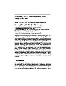
Stock Price Prediction Using K-Nearest Neighbor (kNN) Algorithm

International Journal of Business, Humanities and Technology

Vol. 3 No. 3; March 2013

Stock Price Prediction Using K-Nearest Neighbor (kNN) Algorithm Khalid Alkhatib1 Hassan Najadat2 Ismail Hmeidi 3 Mohammed K. Ali Shatnawi 4 Abstract Stock prices prediction is interesting and challenging research topic. Developed countries' economies are measured according to their power economy. Currently, stock markets are considered to be an illustrious trading field because in many cases it gives easy profits with low risk rate of return. Stock market with its huge and dynamic information sources is considered as a suitable environment for data mining and business researchers. In this paper, we applied k-nearest neighbor algorithm and non-linear regression approach in order to predict stock prices for a sample of six major companies listed on the Jordanian stock exchange to assist investors, management, decision makers, and users in making correct and informed investments decisions. According to the results, the kNN algorithm is robust with small error ratio; consequently the results were rational and also reasonable. In addition, depending on the actual stock prices data; the prediction results were close and almost parallel to actual stock prices.

Keywords: stock price prediction, listed companies, data mining, k-nearest neighbor, non-linear regression. 1. Introduction Recent business research interests concentrated on areas of future predictions of stock prices movements which make it challenging and demanding. Researchers, business communities, and interested users who assume that future occurrence depends on present and past data, are keen to identify the stock price prediction of movements in stock markets (Kim, 2003). However, financial data is considered as complex data to forecast and or predict. Predicting market prices are seen as problematical, and as explained in the efficient market hypotheses (EMH) that was put forward by Fama (1990). The EMH is considered as bridging the gap between financial information and the financial market; it also affirms that the fluctuations in prices are only a result of newly available information; and that all available information reflected in market prices. The EMH assert that stocks are at all times in equilibrium and are difficult for inventors to speculate. Furthermore, it has been affirmed that stock prices do not pursue a random walk and stock prediction needs more evidence (Gallagher and Taylor, 2002; Walczack, 2001; Kavusssanos and Dockery, 2001; Lakonishok et.al, 1994; O'Connor et. al., 1997; Lo and MacKinlay, 1997; Kirt and Malaikah, 1992; Lo and MacKinlay, 1988). Moreover, various studies were performed to determine stock price predictions (Subha and Nambi, 2012; Qian and Rasheed, 2007; Fama and French, 1992; Cochrane, 1988; Campbell, 1987; Chen, et al. 1986; Basu, 1977). In addition to purchasing and selling stocks and shares in stock markets, each stock is not only characterized by its price, but also by other variables such as closing price which represents the most important variable for predicting next day price for a specific stock. There is a relationship and specific behavior exists between all variables that effect stock movements overtime. Different economic factors, such as political stability, and other unforeseeable circumstances are variables that have been considered for stock price predictions (Ou, P. and Wang, H., 2009; Fama and French, 1993; Cochrane, 1988; Campel, 1987; Chen. et.al.1986). Table 1 summarizes the main variables that affect stock movements used in this article. _________________ 1, 3, 4

Department of Computer Information Systems, Jordan University of Science and Technology, Irbid, Jordan Department of Computer Science, College of Computers and Information Technology, Taif University Taif, KSA, and currently on sabbatical leave from Jordan University of science and Technology, Jordan 32 2

© Centre for Promoting Ideas, USA

www.ijbhtnet.com

Data mining technology is used in analyzing large volume of business and financial data, and it is applied in order to determine stock movements. Mining temporal stock markets is required to provide additional capabilities required in cases where the existing data and their interactions need to be observed through time dimension. In stock predictions, a set of pure technical data, fundamental data, and derived data are used in prediction of future values of stocks. The pure technical data is based on previous stock data while the fundamental data represents the companies’ activity and the situation of market. Combining data mining classification approaches in stock prediction yields a future value for each unknown entities of companies’ stocks values based on historical data. This prediction uses various methods of classification approaches such as neural networks, regression, genetic algorithm, decision tree induction, and k-Nearest Neighbors (kNN). In classification approaches, a data set is divided into training data set and testing set. kNN uses similarity metrics to compare a given test entity with the training data set. Each data entity represents a record with n features. In order to predict a class label for unknown record, kNN selects k recodes of training data set that are closest to the unknown records. The rest of the article will be structured as follows; section 2 will exemplify the review of the relevant literature, while section 3 describes the research methodology used and analysis. Section 4 shows the data description, results and analysis. The Non-linear regression results are included in section 5. Finally the conclusion is seen in section 6.

2. Literature Review Financial services companies are developing their products to serve future prediction. There are a large amount of financial information sources in the world that can be valuable research areas, one of these areas is stock prediction and also called stock market mining. Stock prediction becomes increasingly important especially if number of rules could be created to help making better investment decisions in different stock markets. The genetic algorithm had been adopted by Shin et al. (2005); the number of trading rules was generated for Korea Stock Price Index 200 (KOSPI 200), in Sweden Hellestrom and Homlstrom (1998) used a statistical analysis based on a modified kNN to determine where correlated areas fall in the input space to improve the performance of prediction for the period 1987-1996. Both models mentioned were provided in the Zimbabwe stock exchange to predict the stock prices which included Weightless Neural Network (WNN) model and single exponential smoothing (SES) model Mpofu (2004). Clustering stocks approach was provided by Gavrilov et al. (2004) to group 500 stocks from the Standard & Poor. The data represented a series of 252 numbers including the opening stock price. A fuzzy genetic algorithm was presented by Cao (1977) to discover pair relationship in stock data based on user preferences. The study developed potential guidelines to mine pairs of stocks, stock-trading rules, and markets; it also showed that such approach is useful for real trading. Moreover, other studies adopted kNN as prediction techniques such as (Subha et al., 2012; Liao et al. 2010; Tsai and Hsiao 2010; Qian and Rasheed, 2007)

3. Research Methodology And Analysis The kNN algorithm method is used on the stock data. Also, mathematical calculations and visualization models are provided and discussed below. 3.1 k-Nearest Neighbor Classifier (kNN) K-nearest neighbor technique is a machine learning algorithm that is considered as simple to implement (Aha et al. 1991). The stock prediction problem can be mapped into a similarity based classification. The historical stock data and the test data is mapped into a set of vectors. Each vector represents N dimension for each stock features. Then, a similarity metric such as Euclidean distance is computed to take a decision. In this section, a description of kNN is provided. kNN is considered a lazy learning that does not build a model or function previously, but yields the closest k records of the training data set that have the highest similarity to the test (i.e. query record). Then, a majority vote is performed among the selected k records to determine the class label and then assigned it to the query record. The prediction of stock market closing price is computed using kNN as follows: a) Determine the number of nearest neighbors, k. b) Compute the distance between the training samples and the query record. 33



c) Sort all training records according to the distance values. d) Use a majority vote for the class labels of k nearest neighbors, and assign it as a prediction value of the query record. 3.2 Mathematical Calculations and Visualizations Models This represents an overview of equations that were applied in this article for predicting next day price. The calculations includes error estimation, total sum of squared error, average error, cumulative closing price when sorted using predicted values, k-values and training Root Mean Square (RMS) errors. a) Root Mean Square Deviation (RMSD) is accuracy metric that computes the differences between the estimated values, Y, and the actual values, X. The total of RMSD is aggregated into a single value measure. RMSD = SQRT(Y-X)2. b) Explained Sum of Squares (ESS) is computed as follows: ESS = Where yi: is the predicted variable, and y is the actual value. c) Average Estimated Error (AEE) AEE is the total sum of RMS errors for all variables in stock records divided by the total number of the records. AEE = 3.3 Visualization Graph To evaluate the performance of kNN learning model, lift graph is applied and drawn for different companies’ stock values. The lift chart symbolizes the enhancement that a data mining model offers when distinguished against a random estimation, and the change is expressed in terms of lift score. Through contrasting the lift scores for a variety of parts of the data set and for different models, it can then be decided which model is supreme and which percentage of the cases within the data set would gain from employing the predictions model. Furthermore, using the lift chart assist in distinguishing how accurate predictions are for various models with identical predictable characteristic. The lift graph also shows the ratio between the results obtained using the predictive model or not. The other graph applied is the plot curves to show the relation between the actual and predicted stock price.

4. Data Description, Results, And Analysis In this article, data from the Jordanian stock exchange was analyzed and a brief data analysis is presented to provide the reader with the fundamental concepts of data attributes. Also, the obtained results of prediction of the Jordanian stock exchange are provided. 4.1 Data Description

The sample data was extracted from the Jordanian stock exchange. The study sample included stock data of five randomly selected companies listed on the Jordanian stock exchange as a sample training dataset from the period June 4, 2009 to December 24, 2009 as shown in table 2. Each of these companies has approximately 200 records with three attributes including closing price, low price, and high price as shown in table 3. A brief data analysis is presented with the fundamental concepts of data attributes. The attributes for each company are included in the data analysis. Closing price is the main factor that affects the prediction process for a specific stock based on kNN algorithm. The kNN algorithm is applied on a 1000 records to estimate predicted values for each stock. 4.2 Analysis And Results The results of the predicted stock price for each individual company used in the sample with graphs for the actual and predicted prices are presented. The results as seen in tables 4.1 to 4.5 and in figures 1 to 11 are those after applying kNN algorithm for each company's closing prices with the residual values which indicates how far away is the predicted values from the actual values; the negative residual value indicates that the predicted value is larger than the actual one. 34


www.ijbhtnet.com

Section 4.3 summarizes the five companies’ prediction performance. Tables 4.1 to 4.5 respectively represent the results after applying kNN algorithm of the Arab international for education and investment (AIEI), Jordan steel company (JOST), Arab financial investment (AFIN), Irbid district electricity (IREL), and the Arab potash company (APOT). As depicted in the figures (1-10) below, the line chart of the actual and predicted values for the companies in the sample and after adopting the kNN prediction model, the results show that the predictive value and the actual value were moving in similar manner as seen in figure 2,4,6,8, and 10. Moreover, the lift chart also applied to evaluate the performance of kNN learning model used and proved that the model used is performing well; this can also be seen in figures 1,3,5,7, and 9 representing the lift charts (company's dataset). 4.3 Prediction Performance Evaluations Table 6 represents a summary of the total squared errors, RMS errors and the average errors for the five companies. The residuals offer the differences between the predicted values and actual the values in the sample data. The table also shows that the values of errors are very small which indicate that the actual value and predicted value are close. This yields a high accuracy of using the kNN algorithm in predicting stock values.

5. Non-Linear Regression Results Non-linear regression is a data analysis technique in which the observed data is incorporated into a model presented in a mathematical non-linear function combining the model parameters that relies on independent variables used. GraphPad Prism v5.02 software was used to apply centered second order polynomial (quadratic) non-linear regression which has the following formula: Price = B0 + B1 (day – mean (day)) + B2 (day – mean (day))2 Where: B0, B1 and B2: Day: Price:

Constants. Actual day in which we will predict the price. Predicted price depending on the day.

Figure 11 provides a graphical representation of non-linear regression. Also, the figure shows a computed regression equation for each company. These companies are AIEI, JOST, APOT, AFIN, and IREL. Based on these equations, investors can compute the future values of stock prices for each company.

6. Conclusion In this paper, a prediction process for five listed companies on the Jordanian Stock Market was carried out, and is considered to be the first of its type implemented in Jordan as a case study using real data and market circumstances. Consequently, a robust model was constructed for the purpose set out. The data was extracted from five major listed companies on the Jordanian stock exchange, the sample data was used to be our training data set (about 200 records for each company) upon the criteria previously mentioned to apply our model. We adopted an efficient prediction algorithm tool of kNN with k=5 to perform such tests on the training data sets we had. According to the results, kNN algorithm was stable and robust with small error ratio, so the results were rational and reasonable. In addition, depending on the actual stock prices data; the prediction results were close to actual prices. Having such rational results for predictions in specific, and for using data mining techniques in real life; this presents a good indication that the use of data mining techniques could help decision makers at various levels when using kNN for data analysis. So, we consider that employing this prediction model, kNN is real and viable for stock predictions. Nevertheless, the implementation and the full make use of information systems technology and due to the lack of knowledge of financial econometrics in Jordan, there is still long way to utilize advanced predicting models to help the financial markets and brokerage houses and to move forward and be part of the developed international financial markets. Furthermore, this may weakens the attractiveness of investments in the Jordanian market which eventually weakens the market return. The study also shows that contemporary data mining techniques offer the world of finance useful stock market movements' prediction analysis.

35



References Aha, D., Kibler, D.W., Albert, M.K. (1991). Instance-based learning algorithms. Mach Learn, 6, 37–66 Alexander, S.S. (1961). Price movements in speculative markets: Trends or random walks. Ind Manage Rev, 7–26 Breiman, L. (1996). Bagging predictors. Mach Learn 24(2), 123–140 Breiman, L. Friedman, J. Stone, C.J. Olshen, R.A. (1984). Classification and regression trees. Chapman & Hall (Wadsworth, Inc.). NewYork Cao, L. (1997). Practical method for determining the minimum embedding dimension of a scalar time series. Physica D 110, 43–50 Cootner, P.H. (1964.) The random character of stock market prices. MIT Press, MA Corazza, M. Malliaris, A.G. (2002). Multi-fractality in foreign currency markets. Multinat Fin J 6(2), 65–98 Dietterich, T.G. (1997). Machine-learning research: Four current direction. AI Magazine 18(4), 97–136 Dietterich, T.G. (2000). Ensemble methods in machine learning. First International Workshop on Multiple Classifier Systems. New York Fama, E.F. (1965). The behaviour of stock market prices. J. Bus 38, 34–105 Fama, E.F. (1991). Efficient capital markets. II J. Fin. 46(5), 1575–1617 Fama, E.F., Fisher, L., Jensen, M., Roll, R. (1969). The adjustment of stock price to new information. Int. Eco Rev 10(1), 1–21 Frank, R.J., Davey, N. Hunt, S.P. (2000). Input window size and neural network predictors. IEEE-INNS-ENNS Int Joint Conf Neural Netw (IJCNN’00). 2, 2237–2242 Gallagher, L. Taylor, M. (2002). Permanent and temporary components of stock prices: Evidence from assessing macroeconomic stocks. Southern Eco J 69, 245–262 Gately, E. (1996). Neural networks for financial forecasting. Wiley, New York Grech, D. Mazur, Z. (2004). Can one make any crash prediction in finance using the local Hurst exponent idea? Physica A. Statistical Mech Appl. 336, 133–145 Hagan, M.T., Demuth, H.B., Beale, M.H. (1996). Neural network design. PWS Publishing, Boston, MA Hagan, M.T., Menhaj, M. (1994). Training feedforward networks with the Marquardt algorithm. IEEE Trans Neural Netw. 5(6), 989–993 Hansen, L. Salamon, P. (1990). Neural network ensembles. IEEE Trans Patt Analy Mach Intell. 12, 993–1001 Hellstrom, T., Holmstrom, K. (1998). Predicting the stock market. Technical report series IMa-TOM-1997-07. Center of Mathematical Modeling, Malardalen University Hornik, K., Stinchcombe, M., White,H. (1989). Multilayer feed forward networks are universal approximators. Neural Net 2(5), 259–366 Hsieh, D.A. (1991). Chaos and nonlinear dynamics: application to financial markets. J Fin 46, 1839–1877 Hurst, H.E. (1951). Long-term storage of reservoirs: an experimental study. Trans Amer Soc Civil Engi 116, 770–799 Jensen, M.C. (1978). Some anomalous evidence regarding market efficiency. J Fin Eco 6, 95–102 Kavussanos, M.G., Dockery, E. (2001). A multivariate test for stock market efficiency: The case of ASE Applied Financial Economics. 11(5), 573–579(7) Kirt, C.B., Malaikah, S.J. (1992). Efficiency and inefficiency in thinly traded stock markets: Kuwait and Saudi Arabia. J Bank & Fin 16 (1), 197–210 Lo, A.W., MacKinlay, A.C. (1997). Stock market prices do not follow random walks. Market Efficiency: Stock Market Behavior in Theory and Practice 1, 363–389 Mandelbrot, B. (1982). The fractal geometry of nature. W.H.Freeman. New York Mandelbrot, B.B., Ness, J.V. (1968). Fractional brownian motions, fractional noises and applications. SIAM Rev 10, 422–437 May, C.T. (1999). Nonlinear pricing: theory & applications. Wiley, New York Peters, E.E. (1991). Chaos and order in the capital markets: a new view of cycles, prices, and market volatility. Wiley, New York Peters, E.E. (1994). Fractal market analysis: applying chaos theory to investment and economics. Wiley, New York Qian, B., Rasheed, K. (2004). Hurst exponent and financial market predictability. Proceedings of the 2nd IASTED international conference on financial engineering and applications. Cambridge, MA, USA, 203–209 Soofi, A.S., Cao, L. (2002). Modelling and forecasting financial data: techniques of nonlinear dynamics. Kluwer Academic Publishers: Norwell, Massachusetts Walczak, S. (2001). An empirical analysis of data requirements for financial forecasting with neural networks. J Manag Infor Syst 17,4, 203–222

36


www.ijbhtnet.com

Table 1: Stock market variables that affect investor decisions in buy/sell transactions Variable Price Opening Price Closing price High Low

Description Current price Opening price for a specific trading day Closing price for a specific trading day Highest price in a specific day Lowest price in a specific day

Table 2: Companies listed on the Jordanian stock market used in the sample Company Symbol AIEI JOST AFIN IREL APOT

Description The Arab International For Education & Investment. Jordan Steel company Arab Financial Investment Irbid District Electricity The Arab Potash

Number of records 200 200 181 189 200

Table 3: Variables used Variable Name Closing price Low price High price

Description Current price for a stock Lowest price in a specific day for a stock Highest price in a specific day for a stock

Table 4.1: The results after applying kNN algorithm for the (AIEI) Predicted Value 2.85 2.825 2.825 2.9 2.9 2.993333 3 2.91 2.703333 2.703333 2.576364 2.6 2.505 2.555 2.555 2.576364 2.61 2.624 2.61

Actual Value 2.9 2.8 2.85 2.9 2.9 3.03 3 2.91 2.78 2.65 2.67 2.6 2.5 2.55 2.6 2.59 2.61 2.6 2.61

Residual 0.05 -0.025 0.025 0 0 0.036667 0 0 0.076667 -0.053333 0.093636 0 -0.005 -0.005 0.045 0.013636 0 -0.024 0

Predicted Value 2.624 2.64 2.69 2.703333 2.568 2.505 2.443333 2.32 2.42 2.45 2.568 2.443333 2.45 2.443333 2.505 2.568 2.568 2.51 2.42

Actual Value 2.63 2.64 2.69 2.68 2.62 2.5 2.4 2.32 2.42 2.45 2.54 2.48 2.45 2.45 2.5 2.54 2.54 2.51 2.42

Predicted Value 0.006 2.505 0 2.505 0 2.505 -0.023333 2.505 0.052 2.505 -0.005 2.505 -0.043333 2.505 0 2.576364 0 2.505 0 2.576364 -0.028 2.576364 0.036667 2.593333 0 2.576364 0.006667 2.505 -0.005 2.576364 -0.028 2.505 -0.028 2.576364 0 2.56 0 2.505 Residual

Actual Value 2.55 2.5 2.5 2.5 2.5 2.5 2.5 2.55 2.5 2.55 2.55 2.59 2.55 2.5 2.56 2.55 2.55 2.56 2.5

Residual 0.045 -0.005 -0.005 -0.005 -0.005 -0.005 -0.005 -0.026364 -0.005 -0.026364 -0.026364 -0.003333 -0.026364 -0.005 -0.016364 0.045 -0.026364 0 -0.005

Note: AIEI predicted closing prices after applying kNN algorithm. 200 records from the period Jan 4, 2009 to Dec 24, 2009 are selected as the training dataset and only 57 records are shown in the table. Total squared RMS error is 0.263, RMS error is 0.0378 and the average error is -5.434E-09

37



Table 4.2: The results after applying kNN algorithm for Jordan steel company (JOST) Predicted Value 2.47 2.473333 2.47 2.5325 2.615 2.64 2.64 2.64 2.63 2.63 2.63 2.645 2.615 2.64 2.64 2.64 2.675 2.645

Actual Value 2.47 2.47 2.47 2.52 2.58 2.61 2.61 2.65 2.62 2.64 2.62 2.65 2.65 2.63 2.7 2.6 2.67 2.6

Residual 0 -0.003333 0 -0.0125 -0.035 -0.03 -0.03 0.01 -0.01 0.01 -0.01 0.005 0.035 -0.01 0.06 -0.04 -0.005 -0.045

Predicted Value 2.706667 2.69 2.703333 2.672 2.703333 2.69 2.72 2.672 2.63 2.706667 2.79 2.672 2.516667 2.473333 2.516667 2.516667 2.5325 2.5325

Actual Value 2.73 2.69 2.73 2.68 2.66 2.69 2.76 2.65 2.64 2.69 2.79 2.71 2.59 2.47 2.47 2.49 2.51 2.51

Residual 0.023333 0 0.026667 0.008 -0.043333 0 0.04 -0.022 0.01 -0.016667 0 0.038 0.073333 -0.003333 -0.046667 -0.026667 -0.0225 -0.0225

Predicted Value 2.64 2.59 2.672 2.703333 2.755 2.82 2.82 2.962 2.9275 2.923333 2.83 2.8725 2.95 2.9275 2.896667 2.8725 2.923333 2.98

Actual Value 2.68 2.59 2.65 2.72 2.7 2.82 2.83 2.9 2.9 2.92 2.83 2.85 2.94 2.95 2.9 2.93 2.88 2.95

Residual 0.04 0 -0.022 0.016667 -0.055 0 0.01 -0.062 -0.0275 -0.003333 0 -0.0225 -0.01 0.0225 0.003333 0.0575 -0.043333 -0.03

Note: 200 records from the period Jan 4, 2009 to Dec 24, 2009 are chosen as the training dataset and only 57 records are shown in the table. Total squared RMS error is 0.263, RMS error is 0.0378and the average error is 5.4347E-09 Table 4.3: The results after applying kNN algorithm for Arab financial investment (AFIN) Predicted Value 3.396667 3.338 3.431667 3.396667 3.431667 3.413333 3.431667 3.431667 3.49 3.49 3.49 3.338 3.24 3.245 3.24 3.31

Actual Value 3.39 3.39 3.4 3.4 3.4 3.4 3.4 3.4 3.46 3.46 3.46 3.4 3.24 3.24 3.24 3.3

Residual -0.006667 0.052 -0.031667 0.003333 -0.031667 -0.013333 -0.031667 -0.031667 -0.03 -0.03 -0.03 0.062 0 -0.005 0 -0.01

Predicted Value 3.31 3.31 3.24 3.23 3.28 3.356667 3.32 3.245 3.33 3.338 3.295 3.356667 3.338 3.33 3.338 3.295

Actual Value 3.25 3.25 3.24 3.23 3.28 3.36 3.32 3.25 3.27 3.3 3.31 3.31 3.3 3.39 3.3 3.28

Residual -0.06 -0.06 0 0 0 0.003333 0 0.005 -0.06 -0.038 0.015 -0.046667 -0.038 0.06 -0.038 -0.015

Predicted Value 3.36 3.384286 3.36 3.37 3.386667 3.384286 3.4 3.413333 3.396667 3.384286 3.384286 3.413333 3.465 3.384286 3.44 3.465

Actual Value 3.4 3.39 3.32 3.43 3.44 3.33 3.4 3.4 3.4 3.4 3.35 3.44 3.45 3.4 3.44 3.48

Residual 0.04 0.005714 -0.04 0.06 0.053333 -0.054286 0 -0.013333 0.003333 0.015714 -0.034286 0.026667 -0.015 0.015714 0 0.015

Note: AFIN predicted closing prices after applying kNN algorithm. 181 records from the period Jan 4, 2009 to Dec 24, 2009 are chosen as the training dataset and only 54 records are shown in the table. Total squared RMS error is 0.263, RMS error is 0.036 and the average error is -1.005E-08

38


www.ijbhtnet.com

Table 4.4 The results after applying kNN algorithm for Irbid district electricity (IREL) Predicted Value 9.15 8.72 8.803333 9.026667 9.28 9.2 9.026667 8.803333 8.803333 9.026667 9.24 9.1 9.4 8.87 8.87 8.51 8.56 8.56

Actual Value 9.15 8.72 8.81 9 9.28 9.2 9.08 8.8 8.8 9 9.24 9.1 9.4 8.99 8.75 8.51 8.55 8.57

Residual 0 0 0.006667 -0.026667 0 0 0.053333 -0.003333 -0.003333 -0.026667 0 0 0 0.12 -0.12 0 -0.01 0.01

Predicted Value 8.35 8.45 8.1 8.17 8.6 8.45 7.995 8.4 8.29 8.095 8.095 7.825 7.8 7.574615 7.87 7.574615 7.574615 7.8

Actual Value 8.35 8.5 8.1 8.17 8.6 8.4 8.01 8.4 8.29 7.9 8.29 7.95 7.8 7.6 7.87 7.5 7.5 7.8

Residual 0 0.05 0 0 0 -0.05 0.015 0 0 -0.195 0.195 0.125 0 0.025385 0 -0.074615 -0.074615 0

Predicted Value 7.58 7.444 7.574615 7.444 7.41 7.8 7.792 7.8 7.792 8 7.574615 7.346667 7.03 7.433333 7.71 7.574615 7.42 7.07

Actual Value 7.58 7.22 7.5 7.78 7.41 7.8 7.6 7.8 7.6 8 7.74 7.38 7.03 7.4 7.71 7.5 7.42 7.07

Residual 0 -0.224 -0.074615 0.336 0 0 -0.192 0 -0.192 0 0.165385 0.033333 0 -0.033333 0 -0.074615 0 0

Note: AFIN predicted closing prices after applying kNN algorithm. 189 records from the period Jan 4, 2009 to Dec 24, 2009 are chosen as the training dataset and only 54 records are shown in the table. Total squared RMS error is 1.282, RMS error is 0.1046 and the average error is 4.2735E-08 Table 4.5: The results after applying kNN algorithm for The Arab potash (APOT) Predicted Value 33.145 33.82 33.77 34 34.49 34.98 35.166667 34.75 34.99 34.6 34.29 34.825 34.39 34.29 34.533333 34.3 34.435

Actual Value 34.18 33.51 34 34 34.49 34.98 34.87 34.75 34.99 34.6 34.1 34.45 34.39 34.29 34.4 34.3 33.97

Residual 1.035 -0.31 0.23 0 0 0 -0.296667 0 0 0 -0.19 -0.375 0 0 -0.133333 0 -0.465

Predicted Value 32.76 34.29 34.533333 34.01 33.82 33.77 34.833333 34.4 33.525 33.525 33.145 33 33.12 31.6 30.88 29.9 30.4

Actual Value 32.76 34.48 34.05 34.01 33.95 33.54 34.25 34.4 33.51 33 33 33 33.12 31.6 30.88 29.9 30.4

Residual 0 0.19 -0.483333 0 0.13 -0.23 -0.583333 0 -0.015 -0.525 -0.145 0 0 0 0 0 0

Predicted Value 29.97 30.69 30.34 30.36 31.945 32.25 33.145 33.65 32.85 33.11 34.61 34.84 33.525 32.9 31.91 31.945 32.9

Actual Value 29.97 30.69 30.34 30.36 31.9 31.5 32.7 33.3 32.85 33.11 34.61 34.84 33.6 32.9 31.91 31.99 32.9

Residual 0 0 0 0 -0.045 -0.75 -0.445 -0.35 0 0 0 0 0.075 0 0 0.045 0

Note: APOT predicted closing prices after applying kNN algorithm. 200 records from the period Jan 4, 2009 to Dec 24, 2009 are chosen as the training dataset and only 51 records are shown in the table. Total squared RMS error is 22.7453, RMS error is 0.337 and the average error is 2.49E-08

39



Table 6: Prediction performance evaluations for the whole sample companies (five companies) after applying kNN algorithm for k=5 Company AIEI AFIN APOT IREL JOST

Total squared RMS error 0.263151 0.2629177 22.74533 1.2823397 0.17963

kNN algorithm for K = 5 RMS error 0.0378176 0.0363482 0.3372338 0.1046908 0.0300444

Average error -5.43E-09 -1.01E-08 2.50E-08 4.27E-08 1.508E-08

Figure 1 Lift chart for AIEI training dataset

Note: The area between the baseline and the curve is an indicator of the goodness of the model. Figure 2 : Plot graph shows the relationship between AIEI’s predicted/actual closing price for 1 year period 3.2

3

2.8

Predicted Value Actual Value

2.6

2.4

2.2

2 1

40

4

7

10 13 16 19 22 25 28 31 34 37 40 43 46 49 52 55


www.ijbhtnet.com

Figure 3: Lift chart for JOST training data set

Note: The area between the baseline and the curve is an indicator of the goodness of the model. Figure 4: Plot graph shows the relationship between JOST’s predicted/actual closing price for 1 year period 3.2

3

2.8


2.6

2.4

2.2

2 1

4

7

10 13 16 19 22 25 28 31 34 37 40 43 46 49 52 55

Figure 5: Lift chart for AFIN company training data set

Note: The area between the baseline and the curve is an indicator of the goodness of the model.

41



Figure 6: Plot graph shows the relationship between AFIN’s predicted/actual closing price for 1 year period 3.6

3.4


3.2

3 1

4

7

10 13 16 19 22 25 28 31 34 37 40 43 46 49 52 55

Figure 7: Lift chart for IREL company training data set

Note: The area between the baseline and the curve is an indicator of the goodness of the model. Figure 8: Plot graph shows the relationship between IREL’s predicted/actual closing price for 1 year period


9.8 9.6 9.4 9.2 9 8.8 8.6 8.4 8.2 8 7.8 7.6 7.4 7.2 7 6.8 6.6 6.4 6.2 6 5.8 5.6 5.4 5.2 5 1

42

4

7

10 13

16 19

22 25

28 31

34 37

40 43

46 49

52 55


www.ijbhtnet.com

Figure 9 : Lift chart for APOT company training data set

Note: The area between the baseline and the curve is an indicator of the goodness of the model. Figure 10: Plot graph shows the relationship between APOT’s predicted/actual closing price for 1 year period. 35.5 35 34.5 34 33.5 33 Predicted Value Actual Value

32.5 32 31.5 31 30.5 30 29.5 29 1

4

7

10 13 16 19 22 25 28 31 34 37 40 43 46 49 52 55

43

International Journal of Business, Humanities and Technology Figure 11: Regression distributions for the sample companies AIEI, JOST, APOT, AFIN, and IREL.

44
