Structural Observations on Neural Networks for Hierarchically Derived

Structural Observations on Neural Networks for Hierarchically Derived Reproducing Kernels Maia Fraser November 7, 2011

2

Contents 1 Introduction

5

2 Neural Networks for Visual Detection 2.1 Early milestones . . . . . . . . . . . . . . . . 2.2 Recent models for visual selection/detection: 2.3 Focus of this thesis . . . . . . . . . . . . . . . 2.3.1 Reproducing Kernels . . . . . . . . . .

. . . .

. . . .

. . . .

. . . .

. . . .

. . . .

9 . 9 . 10 . 11 . 12

3 CBCL Model 3.1 Background . . . . . . . . . . . . . . . . . . . . . . . . . . . . . . 3.2 The original framework . . . . . . . . . . . . . . . . . . . . . . . 3.2.1 Image patches and transformations . . . . . . . . . . . . . 3.2.2 Neural responses . . . . . . . . . . . . . . . . . . . . . . . 3.3 The CBCL framework . . . . . . . . . . . . . . . . . . . . . . . . 3.4 More detail on the mathematics of this framework . . . . . . . . 3.4.1 Reproducing kernel Hilbert spaces . . . . . . . . . . . . . 3.4.2 L2 -spaces . . . . . . . . . . . . . . . . . . . . . . . . . . . 3.4.3 Abstract derived kernels . . . . . . . . . . . . . . . . . . . 3.4.4 Normalization . . . . . . . . . . . . . . . . . . . . . . . . . 3.4.5 Non-degenerate kernels . . . . . . . . . . . . . . . . . . . 3.5 Universal Axiom for Neural Responses . . . . . . . . . . . . . . . 3.5.1 Aside on Linearity . . . . . . . . . . . . . . . . . . . . . . 3.5.2 Base neural responses . . . . . . . . . . . . . . . . . . . . 3.6 The extended CBCL Framework . . . . . . . . . . . . . . . . . . 3.7 Convolution neural networks and the extended CBCL framework 3.8 Example of convolution neural net to CBCL conversion . . . . . 3.9 Lifting an abstract neural map . . . . . . . . . . . . . . . . . . . e` . . . . . . . . . . . . . . . . . . . . . . . 3.9.1 Injectivity of N 3.10 Templates of the first and second kind . . . . . . . . . . . . . . .

. . . . . . . . . . . . . . . . . . . .

. . . . . . . . . . . . . . . . . . . .

. . . . . . . . . . . . . . . . . . . .

. . . . . . . . . . . . . . . . . . . .

. . . . . . . . . . . . . . . . . . . .

. . . . . . . . . . . . . . . . . . . .

3

. . . .

. . . .

. . . .

. . . .

. . . .

. . . .

. . . .

. . . .

. . . .

. . . .

13 13 13 14 14 14 16 16 18 19 20 21 22 24 26 27 28 33 36 38 38

4

CONTENTS 3.10.1 Using templates of the second kind with linear neural responses . . 3.10.2 Caution regarding templates of the second kind for non-linear neural responses . . . . . . . . . . . . . . . . . . . . . . . . . . . . . . . . 3.11 Closer look at the average neural response . . . . . . . . . . . . . . . . . . 3.11.1 Skipping a layer . . . . . . . . . . . . . . . . . . . . . . . . . . . . 3.12 Underlying neural network . . . . . . . . . . . . . . . . . . . . . . . . . . . 3.12.1 Convolution Neural Networks . . . . . . . . . . . . . . . . . . . . . 3.12.2 General t-filters . . . . . . . . . . . . . . . . . . . . . . . . . . . . .

4 Decomposing and Simplifying 4.1 Initial structural results . . . . . . . . . . . . . . . . . 4.1.1 Assumed architecture . . . . . . . . . . . . . . 4.1.2 Propositions . . . . . . . . . . . . . . . . . . . 4.2 Preliminaries . . . . . . . . . . . . . . . . . . . . . . . 4.2.1 Change of bases . . . . . . . . . . . . . . . . . 4.2.2 Rank . . . . . . . . . . . . . . . . . . . . . . . . 4.2.3 Formal linear dependencies . . . . . . . . . . . 4.2.4 Convenient view of L2 (T ) for finite T . . . . . 4.3 Proof of the Propositions . . . . . . . . . . . . . . . . 4.4 Examples . . . . . . . . . . . . . . . . . . . . . . . . . 4.4.1 Vision example . . . . . . . . . . . . . . . . . . 4.5 Collapsing: general case . . . . . . . . . . . . . . . . . 4.6 Collapsing of the NN’s . . . . . . . . . . . . . . . . . . 4.6.1 Changing kernels vs. changing neural responses 4.6.2 Proof of the Theorem . . . . . . . . . . . . . .

. 39 . . . . . .

39 40 40 43 46 46

. . . . . . . . . . . . . . .

. . . . . . . . . . . . . . .

. . . . . . . . . . . . . . .

. . . . . . . . . . . . . . .

. . . . . . . . . . . . . . .

. . . . . . . . . . . . . . .

. . . . . . . . . . . . . . .

. . . . . . . . . . . . . . .

. . . . . . . . . . . . . . .

. . . . . . . . . . . . . . .

. . . . . . . . . . . . . . .

49 49 49 50 53 53 54 55 56 57 61 66 69 73 73 74

5 Appendix: Distinguishing Ability 5.1 Assumed architecture and matrix notation . . . . . . . . . 5.1.1 Average neural responses . . . . . . . . . . . . . . 5.2 Derived kernels in matrix notation . . . . . . . . . . . . . 5.3 Distinguishing ability of the average neural response . . . 5.3.1 Relationship between W and distinguishing ability

. . . . .

. . . . .

. . . . .

. . . . .

. . . . .

. . . . .

. . . . .

. . . . .

. . . . .

. . . . .

77 77 78 79 79 80

. . . . . . . . . . . . . . .

Chapter 1

Introduction Artificial neural networks have occupied an important place in the field of artificial intelligence (AI) since its early days. As with many tools developed in AI, the motivation has been two-fold: both to achieve capabilities observed in living organisms by emulating (abstracting) the seemingly responsible underlying mechanisms and to understand or validate the role of these mechanisms by observing the success of the tool. An artificial neural network (NN) – an abstraction of a network of biological neurons – is essentially a directed graph, where each node is a computational gate computing a particular function for each of its outgoing arcs (outputs), based on its incoming arcs (inputs). Additionally, however, there are assumed to be some arcs leading into the digraph (representing global input to the NN) and other arcs leading out of the digraph (representing global output of the NN). In general, if there are directed cycles in the graph, the order and tact of computation can be complex to specify. Such NN’s are said to be recurrent. In this thesis, however, we restrict ourselves to feedforward NN’s, where no directed cycles are present. In these NN’s it is understood that the global input values are fed into the feedforward NN at the start, each computational gate waits until all of its inputs have been computed before itself computing, and so on, until finally the global output is obtained. We will allow the values carried by arcs to be real numbers. We will, moreover, assume that each node computes a single output value and that there is only one global output value (i.e. a single top node). Such a feedforward NN may therefore equivalently be viewed as an encoding of a mapping from Rn to R, where n is the number of global input arcs, and the mapping is specified in the form of a circuit (as just described). In other contexts (e.g. the multiclass perceptron) multiple global outputs may be allowed; such feedforward NN’s are equivalent to maps from Rn to Rm . More precisely, this thesis will be concerned with feedforward NN’s used to compute so-called reproducing kernels (which are real-valued). Chapter 2 gives a brief overview of 5

6

CHAPTER 1. INTRODUCTION

the development of such NN models. By NN model is meant a class of NN’s, e.g. those with gates and/or circuits of a prescribed type. Example 1.0.1. [Σ networks] (see [9]). Given a (Borel) measurable function G : R → R and a positive integer r, let Σr (G) denote the class of all maps f : Rr → R, defined (and computed) as p X f (x) = αi G(Ai (x)), ∀x ∈ Rr , i=0

where p ∈ N and for each i, αi ∈ R and Ai : Rr → R is an affine function. By viewing each of the affine functions Ai and the summation procedure as single computational operations, we are also implicitly specifying above how each function in the class Σr (G) is computed. This class may therefore also be seen as an NN model, i.e. class of NN’s: the associated networks are laid out with p gates in the lower layer, each of which has the same r inputs (the coordinates of x), and which compute A1 (x), . . . , Ap (x) respectively, plus a single gate at the top layer which pools the outputs of the lower layer to produce the global output f (x). In this example, Σr (G) represents an NN model, where the circuit topology is fixed and the types of gates is restricted to affine transformations on the lower layer, and summation on the top. Some NN models do not fix the circuit topology absolutely, though they may restrict it. In particular, in some models – for example those discussed in Chapter 2 – the depth of the circuit may be unbounded. Because of the strict sequential order of computation (determined by distance from the global input), it is common to speak of layers in feedforward NN’s; the bottom being the layer where global input arrives and the top being a single node computing the global output (in our case). In general all layers except for the top and bottom are referred to as hidden layers. Networks with few hidden layers (zero or one, typically) are said to be shallow and those with more layers, deep(er). The design issue of shallow vs. deep NN’s has been considered in various cases, going back as far as 1969, when Minsky and Papert showed, in their book Percetrons [13], that a perceptron without hidden layers (the so-called single layer perceptron) cannot compute the XOR function. Several recent papers of Bengio and LeCun, as well as Hinton and some of his students, make the claim that deep NN’s are superior to shallow NN’s in a fundamental way and that shallow NN’s are in this sense inadequate. This claim is sometimes promoted by appealing to H˚ astad’s seminal result in circuit complexity which states that depth-k circuits with only AND, OR or NOT gates must be of exponential size in order to compute the parity function [8]. These are not the gates used in typical NN’s. And there is in fact no existing result in circuit complexity for such general gates and very little work on real circuits at all (what there is usually assumes global input/ouput that is Boolean, allowing only intermediate variables to be possibly real-valued). In order to

7 prove a meaningful result like Haastad’s for the NN setting, one would first need to clearly define the class of real circuits to be considered (specifying the types of computational gates and their computational power) and also define the function to be computed. In this step, the definition of the function must be independent of the design of the circuit. Herein lies the central weakness in the mentioned claims: the function to be computed is defined by an NN and one wishes to consider only NN’s very much like this one - so much like it, in fact, that it seems plausible it is the only one. Such a result would not be a fair analog of Haastad’s. Moreover, H˚ astad’s result is asymptotic while biological circuits have size bounded above by many other natural factors. This is not to say, there is no justification for deep NN’s. Indeed there are likely compelling reasons for nature to form deep circuits, since they are so prevalent. This thesis seeks to understand the role of depth in some NN’s, by showing - at least for a particular class of NN’s - what it does not accomplish. In particular, we show that for the very general model of NN considered here – an extension of the CBCL model – shallow networks produce the same class of mappings as deep networks (see Theorem 4.6.1). Interestingly, our argument against a H˚ astad-like result for that model fails if one strongly restricts the type of transformations from one level to the next of the hierarchy (this will be defined in Chapter 3). Such a restriction is presumably at the core of the pro-deep claims mentioned above and illustrates how sensitive such mathematical results may be to changes in hypotheses. One may in fact regard this thesis as a step towards enunciating and possibly proving the superiority of deep circuits within a certain framework. Indeed, in this thesis we show how to reduce any deep circuit to a shallow one, while making explicit the transformation sets (between levels) which this would imply. If one can rule out such transformation sets then the performed collapsing would be impossible. One crucial issue regarding NN’s that has not been mentioned so far is that of choosing, i.e. learning, a particular instance of an NN model based on known input/output pairs that are in some sense typical of what the NN should produce. This is generally posed as an optimization problem, where one seeks the values of parameters that minimize a cost function (resp. maximize an objective function). More specifically, it is a statistical estimation problem. In any case, the optimization is then solved by a training algorithm. In nature, however, it would necessarily be handled by some form of feedback - growing neurons or losing connections in response to information fed back to the structure. Because the NN’s we have discussed so far have all been feedforward, they can only be tuned in this way by imposing feedback from the outside; backpropagation is a widespread supervised method of this kind. It is worth noting that depth is not usually posed as one of the parameters to learn; typically one learns only the parameters that determine the operations of the gates. But this then forces the designer to make a priori heuristic choices of layers and depth, rather

8

CHAPTER 1. INTRODUCTION

than letting the data determine them. Clearly in nature the entire design - including choice of layers - evolves by a natural process. The resulting development of layers may well be closely related to naturally occurring transformations and the quantities which they leave invariant. Iterative explanations seem most natural: for example, a two layer unit (which will become a building block in larger structures) may only form to detect specific quantities if these quatities exhibit a great deal of invariance to common transformations. Once such sub-units exist, their output may then exhibit invariances which lead to the next level and so on. On the other hand, sub-units which are never used by higher structures may be less likely to persist. Both of these hypothetical development mechanisms involve a form of feedback about topology, but on a different time scale from the feedforward operation of the NN as a mapping. While still remaining within the category of feedforward NN’s this feedback may be incorporated at least into the training of the NN (as with backpropagation): by first learning the layers in an unsupervised way, so as to determine the topology of the NN, and then within that restricted model using labeled data to learn the parameters of gates, by standard supervised methods. In the case of vision, one has fairly strong prior knowledge about what the layers and sub-units should be (based on experimental data), but in more general applications this is no longer the case and flexibility concerning the layers/transformations could be an interesting option to pursue.

Chapter 2

Neural Networks for Visual Detection 2.1

Early milestones

Commonly regarded as a first step in the development of artificial neural networks, the Threshold Logic Unit (TLU) was proposed by McCulloch and Pitts in 1943 [14]. It models a neuron as a computational gate: it takes r inputs (i.e. an r-vector), computes a linear real-valued function (i.e. weighted sum) of the input and then follows this with a thresholding operation (originally a Heaviside function). The inputs and output are assumed to be Boolean. By combining these artificial neurons into networks, it was observed that one may accomplish Boolean AND and OR operations and thus compute any Boolean function. A subsequent milestone was the Perceptron, proposed in 1957 by Rosenblatt [18]. This was essentially a network of TLU’s but with the specification of a particular rule for learning the weights from a training data set, consisting of binary labeled vectors in Rr . Novikov [15] (see also Rosenblatt[19]) proved that this training algorithm will in a finite number of steps find weights for the Perceptron such that it outputs the correct classification for all training data - if such weights exist (i.e. the data is linearly separable). Soon after this result, however, in 1969, came Minsky and Papert’s book on Perceptrons [13]. Among other things, it showed that a Perceptron without hidden layers cannot implement XOR, a result which is widely credited with dampening enthusiasm for NN’s for years afterwards. In 1989, however, Cybenko [4] proved that a multilayer perceptron with one hidden layer can in fact approximate all continuous, real-valued functions to any desired degree of accuracy. The problem with perceptrons however is their fully-connectedness. This means that training for a 32x32 grid, for example, requires learning over 1,000 parameters for 9

10

CHAPTER 2. NEURAL NETWORKS FOR VISUAL DETECTION

each neuron of the hidden layer. Also, invariance to motion – a key feature of biological visual systems – is not built into the perceptron design. In 1980, Fukushima proposed the Neocognitron. This model is very similar to those we will consider in this thesis; it is inspired - as they are - specifically by the pathways of the visual system and addresses the two shortcomings of perceptrons just identified. Its computational gates are of two kinds: S-cells and C-cells. These were intended as models respectively of the simple and complex cells of the visual cortex, which had been identified by Hubel and Wiesel in 1959 [10]. They had observed that the simple cells evolved to detect specific features, such as edges, in restricted parts of the visual field while the complex cells pooled signals from the simple cells to provide position invariant detection, and also additional features such as direction of motion. In the Neocognitron the layers consist alternately of S- and C-cells - a hierarchical architecture originally proposed by Hubel and Wiesel themselves. Only the parameters of the S-cells are learned. The C-cells are always OR gates, whose input is S-cells from various parts of the visual field. These operations - of filtering followed by pooling - are repeated in hierarchical fashion until the entire visual field has been sensed and processed.

2.2

Recent models for visual selection/detection:

One of the key properties of the visual system, which Neocognitron sought to reproduce/explain was translation invariance in object recognition. More general transformationinvariance was also subsequently studied in the neuroscience community [16, 22]. Several computational NN models, aimed at addressing this more general transformation invariance began to appear around 2000. The proposed architectures are similar to Neocognitron but more flexible. They differ slightly but one common ingredient is the idea, introduced in [16], that transformation-invariance could be obtained by pooling over various transformed versions of an object. These models – which are the focus of this thesis – can largely be grouped into two schools. • Poggio and Riesenhuber [17] proposed in 1999 an NN for visual detection in which S-cells and C-cells alternate, but the C-cells perform a max operation (instead of the fixed OR of Neocognitron); this was modified and refined in various papers (for example [20] from 2007) and then Smale et al proposed a mathematical framework which underlies these NN’s in [21] and does not prescribe which type of pooling is done at which layers. We will loosely call such NN’s CBCL Networks. • Bengio and LeCun [11] proposed in 1998 an NN, building on the ideas of LeCun’s earlier NN models [12] from the late 80’s and leading to many variations (in architecture and training) described in subsequent papers. These are generally referred to as Convolution Neural Networks. They alternate linear pooling (“convolution” plus

2.3. FOCUS OF THIS THESIS

11

a bias), and sub-sampling (or max) operations - but in each case these operations are followed by a non-linear activation function (e.g sigmoid) which “squashes” the output before passing it on as input to the next layer. The layers at the end (fully connected without max operations) form essentially a multi-layer Perceptron. As with classic multi-layer Perceptrons (see [3] for a discussion), the learning of these weights is equivalent to logistic regression. Both of these NN models will be considered in more detail in the next Chapter. Similar networks also appeared in the statistical literature around the same time [1, 2]. Amit [2] proposes a depth-limited NN similar to the above but differing in how learning is done. Learning is done separately at the different scales: local features are learned from local image patches, object models are learned from larger image patches. Another related body of work is that on Auto-encoders (Hinton). The underlying network is essentially the same as what we have considered so far; the focus is on training methods for dealing with NN’s with many hidden layers.

2.3

Focus of this thesis

We will not concern ourselves with learning/training algorithms for NN’s in this thesis. Rather we seek to understand purely what can be computed by NN’s of the above two models as a function of different design choices, e.g. depth. NN’s of both models produce similarity measures, so that one obtains an output K(x, y), where y is hard-coded and x is the input. This value should represent how similar the images x and y are. This is sometimes used for classification into n classes c1 , . . . , cn if one has objects y1 , . . . , yn that are known to be “typical” of the respective classes: the class ci which maximizes K(x, yi ) over all i is chosen. Ideally, to support such a procedure there should be a statistical interpretation which allows one to relate K(x, yi ) to a probability that x is in class ci . This statistical aspect is not addressed in the work on CBCL or Convolution Networks, but receives explicit treatment in some statistical approaches [2]. We will not discuss it in this thesis, although a possible conclusion of the present work is that such statistical and learning considerations may be more suited than computability to explain the role of depth. As mentioned, the output of the NN’s we will discuss is typically of the form K(x, y), where x and y are images. In fact, in both Convolution NN’s and CBCL NN’s this output has the structure of a reproducing kernel on the space of images. This observation was first made by Smale et al [21] with regards to CBCL networks. This thesis makes essential use of reproducing kernels to decompose NN’s of the above two models.

12

2.3.1

CHAPTER 2. NEURAL NETWORKS FOR VISUAL DETECTION

Reproducing Kernels

A reproducing kernel is a generalization of an inner product to sets which are not necessarily vector spaces. Definition 2.3.1. Given an arbitrary set X, a map K : X × X → R is said to be a (real-valued) positive definite kernel on X if for any n ∈ N, x1 , . . . , xn ∈ X and a1 , . . . , an ∈ R, n X ai aj K(xi , xj ) ≥ 0. (2.3.1) i,j=1

If in addition the kernel is symmetric, i.e. K(x, x0 ) = K(x0 , x), ∀x, x0 ∈ X, then we call it a reproducing kernel on X. The condition expressed in (2.3.1) is known as Mercer’s condition. Remark 2.3.2. If X is a topological space and K is continuous then K is said to be a Mercer kernel. The nomenclature is somewhat misleading: it is not the Mercer condition which sets a Mercer kernel apart from a reproducing kernel but the added continuity hypothesis. Remark 2.3.3. If X is a real vector space, then a reproducing kernel K(·, ·) on X is an inner product if and only if it is non-degenerate and linear in the first coordinate (hence bilinear), where non-degeneracy means that K(x, y) = 0, ∀y ∈ X if and only if x = 0.

Chapter 3

CBCL Model 3.1

Background

The hierarchical model for deriving reproducing kernels proposed by Poggio and Smale in [21] is based on nested patches of the visual plane v1 ⊂ · · · ⊂ v`−1 ⊂ v` ⊂ · · · ⊂ vd . It generalizes, as well providing a mathematical framework in which to understand, the basic feedforward archictecture for visual processing proposed by Poggio and Riesenhuber several years earlier (in [17]). The term CBCL model is loosely applied to either. This thesis takes advantage of the mathematical structure introduced in [21] to answer certain design questions about the underlying NN’s: specifically it addresses the issues of deep vs. shallow and linear vs. nonlinear neural responses using the geometry of Hilbert spaces and linear algebra.

3.2

The original framework

One assumes a space of images at each layer, denoted Im(v` ), and also spaces H`−1 of transformations between successive layers, where h ∈ H`−1 is a map h : v`−1 → v` . Then, given a reproducing kernel K = K1 at the bottom layer Im(v1 ), kernels are produced in inductive fashion on layers all the way up, till a kernel is obtained on Im(vd ). The recursive step, which computes the kernel on Im(v` ) from the kernel on Im(v`−1 ), is determined by the neural response map. This is a map N` : Im(v` ) → L2 (T`−1 , ν`−1 ), 13

14

CHAPTER 3. CBCL MODEL

which associates to each large-sized image f ∈ Im(v` ) a functional N` (f ) on certain special smaller sized images t ∈ T`−1 ⊂ Im(v`−1 ), called the templates. Then the recurrence is given by: K` (f, g) = hN` (f ), N` (g)iL2 (T`−1 ,ν`−1 ) , ∀f, g ∈ Im(v` ) (3.2.1) where ν` is a measure on T` that has been fixed in advance (for each ` = 1, . . . , d − 1). Definition 3.2.1 (Derived kernel, induced kernel). A reproducing kernel that is obtained by the recurrence (3.2.1) is said to be derived or induced by N .

3.2.1

Image patches and transformations

Certain axioms on the relationship of the Im(v` ) and H` are required as part of the construction: f ◦ h ∈ Im(v`−1 ) if f ∈ Im(v` ) and h ∈ H`−1 . (3.2.2) Moreover, each H` is assumed to be finite and a measure µH ` is fixed on H` .

3.2.2

Neural responses

Two examples of neural responses are considered: Nmax (f )(u) = max K`−1 (f ◦ h, u) h∈H

and Navg (f )(u) =

X

µH `−1 (h)K`−1 (f ◦ h, u)

h∈H

where u is an arbitrary element of Im(v`−1 ), or of a finite template set T`−1 ⊂ Im(v`−1 ). Navg is referred to as a weighted average. Note that it makes use of the postulated measures µH ` on the sets H` .

3.3

The CBCL framework

While the description of the mathematical framework given above and in [21] is tied to visual processing, the framework is applicable much more widely. In the original paper, besides visual processing, text processing is also considered (the model is used to produce reproducing kernels on character strings). Moreover, the work in this thesis began during a visit to Smale in Hong Kong in the summer of 2010, as preparation for an application in bioinformatics. The goal was to use the same framework to develop a reproducing kernel on strings of amino acids, which would predict pairs of peptides likely to provoke similar immune responses. In all these applications there are certain commonalities.

3.3. THE CBCL FRAMEWORK

15

We therefore present here a slightly more abstract version of the framework of [21] which applies to all these settings and which we will use throughout the remainder of the thesis. We refer to this as the “CBCL framework” from now on. It is a mathematical framework, as in [21], for hierarchically deriving a reproducing kernel. This may be viewed as a computation performed by an NN. We will use the term “CBCL model” to refer to the underlying NN model. Definition 3.3.1 (CBCL Framework). Instead of using visual patches and image spaces which consist of functions (denoted f, g etc..) on these patches, we start with simpler and more general data: • sets Xd , . . . , X2 , X1 (whose elements we denote for example x), • for each ` = 2, . . . , d a finite set H` of maps from X` to X`−1 , called transformations and a probability measure µH` on H` , • for each ` = 1, . . . , d − 1 a finite set T` ⊂ X` of templates and a probability measure ν` on T` , • a reproducing kernel K1 on X1 . We then use the same recursion as before, given by (3.2.1), and the same neural responses, Nmax or Navg , though from time to time it will also be useful to consider arbitrary neural responses N` : X` → L2ν`−1 (T`−1 ). Using the new notation, the standard neural responses (from the `’th layer to the (` − 1)’th) are as follows: Nmax (x)(t) = max K`−1 (h(x), t) h∈H

and Navg (x)(t) =

X

µH `−1 (h)K`−1 (h(x), t),

h∈H

for x an arbitrary element of X` and t an arbitrary element of X`−1 (or of a finite template set T`−1 ⊂ X`−1 ). Warning: The sets X` correspond to the sets Im(v` ) of the orginal framework. However, H` in the original framework was a subset of Maps(Im(v`−1 ) → Im(v` )). These maps were used only to convert elements of Im(v` ) to elements of Im(v`−1 ). This was done by precomposition (i.e. pull-back): x ∈ Im(v` )

x ◦ h ∈ Im(v`−1 ),

16


which amounts to picking out a particular small image from within a large one. We are now retaining only this conversion aspect, and taking H` to be a set of maps from X` to X`−1 , i.e. now H` is a subset of Maps(X` → X`−1 ).

3.4

More detail on the mathematics of this framework

Before we go further, we look in more detail at the mathematical objects and constructions in this framework. First we look at the two types of Hilbert spaces used: reproducing kernel Hilbert spaces and L2 spaces. Then we look at how they are used.

3.4.1

Reproducing kernel Hilbert spaces

We refer to Cucker and Smale’s paper [5] Chapter III, for a more detailed discussion of relevant results on reproducing kernel Hilbert spaces. The essential ingredients we will use are given in their Theorem 2 in that Chapter. Paraphrased, it is as follows. Given a set X with a reproducing (i.e. symmetric and positive definite) kernel K : X × X → R (see Definition 2.3.1), there is a unique Hilbert space HK of functions on X such that • span{Kx | x ∈ X} is a dense subset of HK , and • f (x) = hKx , f iHK for all f ∈ HK , where for all x ∈ X, Kx is defined to be the function K(x, ·). The space HK is said to be a reproducing kernel Hilbert space (RKHS). Suppose we associate to each x ∈ X the map Fx (f ) := f (x). Then Fx (f ) = hKx , f iHK and so Fx is necessarily a continuous linear functional on HK (by the properties of the inner product and its induced metric). Conversely, an arbitrary Hilbert space H of functions on a space X is called a reproducing kernel Hilbert space if for each x ∈ X, the so-called evaluation map Fx defined by Fx (f ) = f (x) is continuous (i.e. if for each x ∈ X there exists Mx > 0 such that |Fx (f )| = |f (x)| ≤ Mx ||f ||H for all f ∈ H). In this case, the Riesz representation theorem produces for each x ∈ X the unique Kx such that Fx (f ) = hKx , f iH for all f ∈ H. One may then define K(x, y) to be hKx , Ky iH and verify that this is a reproducing kernel on X. Moreover, H is then exactly the HK defined above. We remark that the construction in [5] also deals with the continuity of the elements of HK as functions on X and it assumes both that X is a compact topological space and that K is a Mercer kernel (i.e. continuous, in addition to being symmetric and positive definite). However, the well-definedness of the Hilbert space HK and the continuity of Fx as a linear functional on HK do not require either of these additional properties.

3.4. MORE DETAIL ON THE MATHEMATICS OF THIS FRAMEWORK

17

Indeed, if a Hilbert space of real-valued functions on X satisfies the above conditions then it is the completion of the inner product space span{Kx | x ∈ X} whose inner product is defined by linearly extending hKx , Ky i = K(x, y). We refer to HK as the reproducing kernel Hilbert space associated to K and denote by h·, ·iHK its inner product (obtained as just mentioned). The feature map Φ Given a space X with reproducing kernel K(·, ·) and associated Hilbert space HK , define a map Φ : X → HK by Φ : x 7→ Kx . This is called the feature map for the kernel K (and Hilbert space HK ). When we have several spaces Xi , each with a kernel Ki (·, ·), as is the case when using the CBCL framework, we will denote by Φi the feature map for Ki (·, ·). Note on positive definiteness vs. positive semidefiniteness Recall the definition of a reproducing kernel as a symmetric, positive definite kernel (see Definition 2.3.1), where positive definiteness means: for all n ∈ N, for all x1 , . . . , xn ∈ X and for all a1 , . . . , an ∈ R, n X

ai aj K(xi , xj ) ≥ 0.

(3.4.1)

i,j=1

While this condition is equivalent to the matrix M = (K(xi , xj )) being positive semidefinite for any choices of m ∈ N and x1 , . . . , xm ∈ X, it in fact results in a positive definite bilinear form on the appropriate vector space of functions on X (see Lemma 3.4.1 below). Essentially this happens because the feature map Φ : x 7→ Kx from X to span{Kx | x ∈ X} sends all x such that K(x, x) = 0 to the zero function. More precisely, if we define a bilinear form h·, ·i on span{Kx | x ∈ X} by setting hKx , Ky i := K(x, y) and extending bilinearly, the Lemma says this form is positive definite.1 This makes h·, ·i an inner product (as its symmetry and linearity are immediate). 1

Note that we may view HK as R/R0 where R ⊂ RX consists of vectors which have only finitely many nonzero entries and R0 consists P of such vectors which represent the zero function on X via K (i.e. via Φ), namely R0 = {(αx )x∈X | x∈X αx Kx = 0}. The Lemma is a general fact about bilinear forms b(·, ·) defined using a semi-definite matrix. A priori we have such a bilinear form on R (corresponding to the form h·, ·i defined above). The Lemma says that all vectors ze ∈ Zb = {z | b(z, z) = 0} are automatically in the kernel of b (recall ker b consists of those vectors z for which b(z, y) = 0, ∀y ∈ X) and thus these two sets are equal. This means that when we quotient by R0 , which is ker b, then we are in fact quotienting by Zb and thus we obtain a nondegenerate bilinear form on the quotient space.

18


Lemma Pm 3.4.1. Given a reproducing kernel K on the space X and an arbitrary element z = i=1 βi Kxi in span{Kx | x ∈ X} such that hz, zi = 0, it follows that z(y) = 0 for all y ∈ X, i.e. z is the zero function on X. P Pm Pm Proof. Suppose h m i=1 βi Kxi , j=1 βj Kxj i = 0, i.e. that i,j=1 βi βj K(xi , xj ) = 0. If there exists y ∈ X such that z(y) = R 6= 0, then write xm+1 = y, αm+1 = 1, and αi = αβi for 1 ≤ i ≤ m, where α < −

K(y, y) 2R

if R > 0,

α > −

K(y, y) 2R

if R < 0.

or

Note that R = z(y) = m+1 X

Pm

i=1 βi K(xi , y).

αi αj K(xi , xj ) = α

2

i,j=1

= 2α

m X

We have

βi βj K(xi , xj ) + 2α

i,j=1 m X

m X

βi K(xi , y) + K(y, y)

i=1

βi K(xi , y) + K(y, y)

i=1

= 2αR + K(y, y) < −K(y, y) + K(y, y) = 0, which contradicts (3.4.1).

3.4.2

L2 -spaces

Given a measure space (T, µ), we denote by L2 (T, µ) or L2µ (T ) the Hilbert space of “square integrable functions” on T . This is the completion of the standard inner product space obtained by defining  1 2 Z   hf, gi := f gdµ T

for all f, g in the normed vector space of “square integrable functions” on T. The elements of this vector space are equivalence classes of functions on T for the relation f ∼ g ⇔ ||f − g||2 = 0,

3.4. MORE DETAIL ON THE MATHEMATICS OF THIS FRAMEWORK where

19

 1 2 Z 2   . ||f ||2 := |f | dµ X

In this quotient space || · ||2 then defines a norm. We remark that there is a natural embedding of HK` in L2 (Im(v` )). See Cucker and Smale [5] for a discussion of this. Actually, in our framework T will be a finite set of templates, so we may replace the above integrals with weighted sums. Remark 3.4.2. We may sometimes omit mention of the measure µ when this is clear from the context or irrelevant; then we simply write L2 (T ).

3.4.3

Abstract derived kernels

We make the following abstract observation. Let X and Y be two sets and φ : X → Y . Suppose that Y is equipped with a reproducing kernel K (see Definition 2.3.1). For example, if Y is a Hilbert space, then the inner product on Y is a reproducing kernel. Then we can define a reproducing kernel on X by pulling K back: Proposition 3.4.3. The map φ∗ K : X × X → R defined by φ∗ K(x1 , x2 ) = K(φ(x1 ), φ(x2 )) is a reproducing kernel on X. Suppose X and Y are in fact vector spaces and K is an inner product on Y . Then if the map φ is linear and injective, the form φ∗ K will be an inner product on X. On the other hand, linearity of φ and non-degeneracy of φ∗ K together will imply injectivity of φ, while surjectivity of φ and bilinearity of φ∗ K will imply linearity of φ. Proof of Proposition 3.4.3. The symmetry and positive definiteness of φ∗ K follow immediately from the symmetry and positive definiteness of K. In the case where Y is a vector space with inner product K, then linearity of φ implies bilinearity of φ∗ K and injectivity of φ implies nondegeneracy of φ∗ K thus making it an inner product on X. Suppose φ is linear but not injective and let x1 , x2 be two distinct elements of X such that φ(x1 ) = φ(x2 ). Then φ∗ K(x1 − x2 , x1 − x2 ) = K(0, 0) = 0 and yet x1 − x2 6= 0. Suppose φ is surjective and φ∗ K is bilinear. Then for any x1 , x2 , z ∈ X, φ∗ K(x1 + x2 , z) = φ∗ K(x1 , z) + φ∗ K(x2 , z) = K(φ(x1 ), φ(z)) + K(φ(x2 ), φ(z)) = K(φ(x1 ) + φ(x2 ), φ(z)) while φ∗ K(x1 + x2 , z) = K(φ(x1 + x2 ), φ(z)) by definition. Thus, K(φ(x1 + x2 ), φ(z)) = K(φ(x1 )+φ(x2 ), φ(z)). Since this holds for all φ(z) and φ is surjective, we have φ(x1 +x2 ) = φ(x1 ) + φ(x2 ) by the non-degeneracy of K.

20


The above construction of pullback kernel is exactly that used in the recurrence (3.2.1). Proposition 3.4.3 shows this indeed yields a reproducing kernel.

3.4.4

Normalization

In practise, one may wish to use normalized neural responses, so that the derived kernel has values between −1 and 1 and K2 (x, x) = 1 for all x ∈ X2 . We remark that the latter condition implies the former. Lemma 3.4.4. If K is a reproducing kernel on X such that K(x, x) = 1, ∀x ∈ X, then −1 ≤ K(x, y) ≤ 1, ∀x, y ∈ X. Proof. This is a consequence of the Cauchy-Schwarz inequality for positive definite kernels. To give a direct proof, take x1 , x2 ∈ X arbitrary and α1 = α2 = 1. Then the positive 2 P definite condition implies αi αj K(xi , xj ) ≥ 0. So, i,j=1

K(x1 , x1 ) + K(x2 , x2 ) + 2K(x1 , x2 ) ≥ 0 2 + 2K(x1 , x2 ) ≥ 0 K(x1 , x2 ) ≥ −1. On the other hand, by taking α1 = 1, α2 = −1 we obtain 2 − 2K(x1 , x2 ) ≥ 0 so K(x1 , x2 ) ≤ 1. In order to obtain a normalized version of a neural response N : X2 → L2 (T ), it therefore suffices to multiply, for each x ∈ X2 , the value of N (x) by a scalar α(x) that is chosen so that hα(x)N (x), α(x)N (x)iL2 (T ) = 1. Definition 3.4.5 (Normalized neural response). Specifically, given a neural response N : ˆ is defined by X2 → L2ν (T ), the normalized neural response, denoted N ˆ (x)(t) = α(x)N (x)(t), ∀x ∈ X2 , ∀t ∈ T, N where !1/2 1/α(x) = ||N (x)||L2ν (T ) =

X t∈T

(assuming finite T ).

ν(t)[N (x)(t)]2

3.4. MORE DETAIL ON THE MATHEMATICS OF THIS FRAMEWORK

3.4.5

21

Non-degenerate kernels

Given a finite set X, consider the Hilbert space L2 (X) (defined using the empirical, i.e. uniform, measure on X). L2 (X) consists of all real-valued functions on X and for any two such functions, f and g, we have hf, giL2 (X) :=

X 1 f (x)g(x), N

x∈X

|X| where N = P|X|. Or alternatively, one could consider R 2with the standard dot product u · v := ux vx ; this Hilbert space is isomorphic to L (X). By Section 3.4.1, there x∈X

exists a reproducing kernel K(·, ·) on X such that L2 (X) = HK . This is because L2 (X) is finite dimensional and so the evaluation map Fx defined by Fx (f ) = f (x), being linear, is necessarily continuous. Lemma 3.4.6. The associated feature map Φ : X → L2 (X) is injective and in fact all Φ(x), x ∈ X are linearly independent. The function Φ(x) = KX takes on the value 1 on x, and 0 on all other y ∈ X. We give the proof for L2 (X) as stated, but the proof goes through for any isomorphic Hilbert space (for example R|X| ). Proof. If

M P

ai Kxi = 0 for some M ∈ N, a1 , . . . , aM ∈ R, and distinct x1 , . . . , xM ∈ X

i=1

then h

M P

ai Kxi , f iL2 (X) = 0 for all functions f on X, which, by the reproducing property,

i=1

is equivalent to

M P

ai f (xi ) = 0 for all functions f on X, and therefore implies ai = 0, ∀i

i=1

because we can for example take f such that f (xi ) = ai . Now, given x, x0 ∈ X, let f, f 0 be the functions which are 1 on x, respectively on x0 , and 0 elsewhere, then f = Kx , f 0 = Kx0 and thus K(x, x0 ) = hf, f 0 iL2 (X) . Indeed f (y) = 0 for y 6= x means hf, Ky iL2 (X) = 0 by the reproducing property, so f ∈ span(Kx ) (i.e. f is a multiple of Kx ) and therefore f = Kx because f (x) = hf, Kx iL2 (X) = 1. Definition 3.4.7 (Non-degenerate kernel). We call a kernel K on a finite set X nondegenerate if dim HK = |X|.

22


We have given one example of a non-degenerate kernel K, with L2 (X) as its RKHS. All non-degenerate kernels on a finite X have RKHS of same dimension, i.e. have isomorphic RKHS’s. Lemma 3.4.6 may be applied to any of them. Now given an arbitrary kernel K 0 on X, its reproducing kernel Hilbert space HK 0 is isomorphic to a subspace of L2 (X), since dim HK 0 is at most the dimension of L2 (X), namely |X|, and these are finite-dimensional Hilbert spaces. Let Θ : HK 0 → L2 (X) be such an injective isometry. Then we may define Ψ := Θ ◦ ΦK 0 which is a map Ψ : X → L2 (X). We observe K 0 (x, x0 ) = hΨ(x), Ψ(x0 )iL2 (X) for all x, x0 ∈ X. Indeed: hΨ(x), Ψ(x0 )iL2 (X) = hΘ ◦ ΦK 0 (x), Θ ◦ ΦK 0 (x0 )iL2 (X) = hΦK 0 (x), ΦK 0 (x0 )iHK 0 = K 0 (x, x0 ). So, Lemma 3.4.8. All reproducing kernels on X are pullbacks of the inner product in L2 (X). Alternatively, any reproducing kernel K satisfies: K(x, x0 ) = Θ(x) · Θ(x0 ) where Θ is some map Θ : X → R|X| , and the operation on the right hand side is the Euclidean dot product. Remark 3.4.9. Another related observation is that any Hilbert space H of functions on a finite set X is isomorphic to a subspace of L2 (X) since dim H ≤ dim L2 (X) < ∞.

3.5

Universal Axiom for Neural Responses

The recurrence (3.2.1) and the neural responses of the CBCL framework are similar to the recurrence and neural responses of convolution networks. We formalize this similarity in terms of an axiom which both frameworks satisfy. We then define an extension of the CBCL framework (the “extended CBCL framework”) – in terms of this Axiom. It encompasses convolution neural networks and CBCL networks. In Chapter 4, we show that any hierarchy of the extended CBCL framework can be decomposed into simple pieces and its depth thus reduced.

3.5. UNIVERSAL AXIOM FOR NEURAL RESPONSES

23

Recursion To avoid excess notation we specialize to layers 1 and 2, and drop subscripts. Then in both cases (CBCL and convolution networks - see Section 3.7 for a discussion of the latter) we have a recurrence of the form, K2 (x, x0 ) := hN (x), N (x0 )iL2 (T1 )

(3.5.1)

for x, x0 ∈ X2 with neural response N : X2 → L2 (T1 ). The induced K2 (·, ·) is indeed a reproducing kernel by Proposition 3.4.3. In fact it would still be one if we were to pull back a reproducing kernel defined on an arbitrary space of functions on T1 (instead of the standard inner product on L2 (T1 )); however, we will not need this generality. See also the comment in Section 3.5.3. In both models, the neural responses N and kernels K1 satisfy the following axiom2 : Axiom 3.5.1. All the functions in N (X2 ) ⊂ L2 (T1 ) are of a special form, namely for each x2 ∈ X2 there exists Nbase (x2 ) ∈ Maps(X1 → HK1 ) such that, N (x2 )(t) = hNbase (x2 )(t), K1,t iK1 = Nbase (x2 )(t)(t), ∀t ∈ T1 .

(3.5.2)

This means that evaluation of the elements of N (X2 ) ⊂ L2 (T1 ) on points of T1 is done using the inner product of HK1 and equation (3.5.2) specifies exactly how. This formula will be essential to what we do in the remainder. Remark 3.5.2. In fact the axiom also provides a way to define the values of N (x2 ) on all elements of X1 (not just the particular subset T1 ⊂ X1 ). Remark 3.5.3 (Generality of the Axiom and the space of functions on T1 ). The above Axiom is quite weak. Let N be an arbitrary map N : X2 → L2 (T1 ) and assume that for each t ∈ T1 , K1,t is not the zero function on X1 . Then we claim that N satisfies Axiom 3.5.1. In practice, most neural responses are defined directly in terms of elements of HK1 so the Axiom is immediately verified. In this sense it serves mainly as a comment on the means of definition. Its use as an axiom is in allowing us to formalize the notion of linearity of neural responses. We do this is Section 3.5.1. We now prove the claim. Let N be given and assume the stated nondegeneracy hypothesis on K1,t for each t ∈ T1 . Define Nbase ∈ Maps(X1 → HK1 ) as follows. For each t ∈ T1 , let y(t) ∈ X1 such that K1 (t, y(t)) 6= 0. For each x2 ∈ X2 and t ∈ T1 , set, Nbase (x2 )(t) :=

N (x2 )(t) K ∈ HK1 . K1 (t, y(t)) 1,y(t)

2 The reader may easily verify this for the CBCL model; we show it for convolution neural networks in Section 3.7.

24


0 And for x1 ∈ X1 \ T1 define Nbase (x2 )(x1 ) ∈ HK1 arbitrarily. Then, for all x2 ∈ X2 and t ∈ T1 we have,

Nbase (x2 )(t)(t) =

N (x2 )(t) N (x2 )(t) K1,y(t) (t) = K1 (t, y(t)) K1 (t, y(t)) K1 (t, y(t)) = N (x2 )(t),

so N indeed satisfies Axiom 3.5.1. A second consequence of the above construction is the following. Assume T1 is finite. Had we postulated an arbitrary Hilbert space of functions F(T1 ) on T1 in the recursion and Axiom, we could replace F(T1 ) by L2 (T1 ) and replace N : X2 → F(T1 ) by N 0 : X2 → L2 (T1 ) where N 0 (x2 ) = Θ(N (x2 )) for all x2 ∈ X2 with Θ : F(T1 ) → L2 (T1 ) being an isometry that embeds the Hilbert space F(T1 ) in L2 (T1 ) (such an isometry must exist since dim F(T1 ) ≤ |T1 | = dim L2 (T1 ) < ∞). Then, using the above construction, one sees that the new N 0 would still satisfy Axiom 3.5.1. Its derived kernel would be the same as that derived by N since Θ is an isometry. Thus, we have lost no generality in restricting ourselves to F(T1 ) = L2 (T1 ).

Axiom 3.5.1 can be re-expressed by saying, N factors through Maps(X1 → HK1 ): N

X2

- F(T1 ) -

N

al ev

ba se

-

Maps(X1 → HK1 ) Here the map “eval” is evaluation using the inner product of HK1 . Specifically given f ∈ Maps(X1 → HK1 ) and x1 ∈ X1 , it is defined by (eval f )(x1 ) = hf (x1 ), K1,x1 iK1 .

3.5.1

Aside on Linearity

Definition 3.5.4 (Linear Neural Responses). When for each x2 ∈ X2 , Nbase (x2 )(x1 ) ∈ HK1 is constant as a function of x1 ∈ X1 , then we say the neural response N is linear. In the alternate terminology given above, this corresponds to N factoring through

3.5. UNIVERSAL AXIOM FOR NEURAL RESPONSES

25

constant maps, CMaps(X1 → HK1 ) ∼ = HK1 : X2

N

- F(T1 ) -

N

al ev

ba

se

-

CMaps(X1 → HK1 ) ∼ = HK1 Remark 3.5.5. This definition is consistent with the common CBCL usage of linear neural response; the average neural response is linear by this definition and the max is not. Moreover, as we will see, the neural responses of convolution neural networks which use a non-linear activation function (i.e.squashing function) are in general non-linear. The justification for this terminology is that upon applying “eval” to a constant map, the element of L2 (T1 , ν1 ) that one obtains is actually just the restriction to T1 of an element of the Hilbert space HK1 (i.e., it is a linear functional on Φ1 (T1 )): f ∈ CMaps(X1 → HK1 ) s. t. (∀x1 ∈ X1 )f (x1 ) = F ∈ HK1 ⇒ (eval f )(x1 ) = hF, K1,x1 iK1 = F (x1 ) where the last equality follows from the reproducing property of HK1 . Note that in fact the element obtained is exactly F itself. Remark 3.5.6. By abuse of notation, in the case of linear neural responses we will consider Nbase to be a map into HK1 itself (not the isomorphic space CMaps(X1 → HK1 )): given x2 ∈ X2 , Nbase (x2 ) ∈ HK1 is just the element F mentioned above (i. e. the constant value in HK1 to which the true Nbase (x2 ) is equal for all x1 ∈ X1 ). Example 3.5.1. To give two concrete examples, max Nbase (x)(t) = max K1,ht (x) , h∈H

where ht is the element of H for which K1 (h(x), t) is maximized, and avg Nbase (x)(t) =

X

µH `−1 (h)K1,h(x) .

h∈H max (x)(t) corresponds depends on t. In In the first case, the element of HK1 to which Nbase max the second case, it does not. Nbase is therefore not linear, whereas N avg is linear.

26


Example 3.5.2. For a simple (toy) example of a linear neural response, not a priori expressed as a weighted average, consider the kernel K on the set X1 = {a, b} given by ( K(i, j) =

1 if i = j, 0 otherwise

Let X2 = [0, 1], the closed unit interval, and define a neural response Nbase by Nbase (x) = xKa + (1 − x)Kb for each x ∈ X2 . Then Nbase defines a linear neural response since for each x ∈ X2 , Nbase (x) is an element of HK .

3.5.2

Base neural responses

We now look at Axiom 3.5.1 more closely. Proposition 3.5.7. Assume Axiom 3.5.1. Nbase and T1 uniquely determine N . As a partial converse, if span of {K1,t : t ∈ T } is equal to all of HK1 and N is linear, then Nbase is uniquely determined. Proof. The first direction is trivial: suppose we are given Nbase and T1 , then Axiom 3.5.1 defines N (x2 )(t) = hNbase (x2 )(t), K1,t iK1 . 0 Now suppose N linear satisfies the axiom and there are Nbase and Nbase such that 0 hNbase (x2 ), K1,t iK1 = N (x2 )(t) = hNbase (x2 ), K1,t iK1 0 (x2 ) by the nondegeneracy of the inner product and for all t ∈ T1 . Then Nbase (x2 ) = Nbase the fact that the K1,t span HK1 .

Definition 3.5.8. Given N and Nbase satisfying Axiom 3.5.1, we call Nbase a base neural response for N . Given a base neural response Nbase and a choice of template set T1 we call N the neural response associated to Nbase and T1 . and denote it ρT1 (Nbase ): ρT1 (Nbase ) : X2 → L2 (T1 ). We have ρT1 (Nbase )(x2 )(t) = Nbase (x2 )(t)(t) for all x2 ∈ X2 , t ∈ T1 . Note that ρT1 is thus a functional which takes a map Nbase : X2 → Maps(X1 → HK1 ) to a map N = ρT1 (Nbase ) : X2 → L2 (T1 ). When the dependence of L2 (T1 ) = L2 (T1 , ν1 ) on ν1 needs to be made explicit, we will write ρT1 ,ν1 .

3.6. THE EXTENDED CBCL FRAMEWORK

3.6

27

The extended CBCL Framework

Definition 3.6.1 (Extended CBCL Framework). The extended CBCL framework is exactly as the CBCL framework, with spaces X1 , . . . , Xd (see Definition 3.3.1), except that: • a given layer may have several kernels, K`1 , . . . , K`s , (all on X` ) and corresponding 1 , ν 1 ), . . . , L2 (T s , ν s ), neural responses N`1 , . . . , N`s into Hilbert spaces L2 (T`−1 `−1 `−1 `−1 and • each Kì satisfies a recursion of the form Kì (x, x0 ) = hN`1i (x), N`1i (x0 )iL2 (T 1i ,ν 1i ) + . . . `

`

. . . + hN`ri (x), N`ri (x0 )iL2 (T ri ,ν ri ) , `

`

1i , . . . , K ri are the kernels on level ` − 1 and each neural for x, x0 ∈ X` , where K`−1 `−1 ji . response N`ji satisfies Axiom 3.5.1 for lower kernel K`−1

Notation: The number r = ri of lower layer kernels may also depend on i, but we have reduced the notation. Moreover, when dealing with a single kernel Kì with i fixed, we will omit the superscript i in the names of neural responses, and lower level templates and kernels which are used to construct Kì . Note that, given s kernels K`1 , . . . , K`s at the layer i `, such that Ps the i’th kernel K` depends on ri kernels at the layer ` − 1, there will in total be S = i=1 ri kernels at layer ` − 1 (and this S will play the role of s when we recurse again). We call the underlying model of NN the extended CBCL model. It is described, along with the CBCL model, in Section 3.12. Remark 3.6.2. We note that N`ji is not restricted in any other way in this framework (besides satisfying Axiom 3.5.1). One may for example define N`ji as a weighted average using an arbitrary transformation set H ji and/or weights µji (h) ∈ R. This is technically allowed in the CBCL model as well, though usually the transformations and weights there are viewed as having some physical meaning. As mentioned in Section 3.5.1, for a linear neural response N2 which satisfies Axiom 3.5.1, one may always assume that N (x2 ) – as a set of functions on T1 – is given by linear functionals on HK1 . Their Riesz representatives then span a vector subspace of HK1 . It will be convenient to view this subspace as carrying a different inner product, namely, the one inherited from L2 (T1 ), instead of the standard inner product on HK1 .

28


3.7

Convolution neural networks and the extended CBCL framework

We abbreviate these CNN’s. As remarked in Chapter 2, their lower (not fully-connected) layers alternate so-called convolution layers and max or sub-sampling layers. In each of those layers, the named operation (convolution, max, sub-sampling) is typically followed by an additional function before the output of the layer is produced and may serve as input for the next layer. The additional function is either a “squashing” function (a.k.a. “activation function”) - typically a sigmoid - or addition of a bias term (constant) followed by a squashing function. We will consider it to be the identity function if no such additional function is present. We claim each of the named operations (convolution, max, sub-sampling) is in fact a weighted average or max as defined above for the CBCL model but that when it is followed by the additional function (squashing or addition of bias and then squashing) we may handle this with a neural response which still satisfies Axiom 3.5.1. Thus the lower (non fully-connected) part of a CNN may be viewed as an extended CBCL NN. The remainder of this Section explains this conversion. CNN’s We look first at convolutions. Given an input image x whose pixels are labeled by the square grid [−m, m] × [−m, m], a convolution (in LeNet, for example) produces as output several feature vectors y k , k ∈ K for each of which the i’th pixel, i ∈ [−p, p] × [−p, p], is X yik = Whk · [subi (x)]h . h∈H

Here the set H = [−n, n] × [−n, n] is specifically a grid, subi (x) denotes a subimage of x centered at the i’th pixel, and [subi (x)]h denotes the h’th pixel of subi (x). We are assuming that m > n is sufficiently large that all the subimages subi (x) of x, for i ∈ [−p, p] × [−p, p], are well-defined3 . Each of the feature vectors y k uses the same input x (and same “receptive field’) and each is followed by addition of a bias term and application of a sigmoid function. The pixels of each feature vector are said to form a “plane”. LeNet learns the weights Wh and also the bias term b which will be added before a sigmoid function is applied. In the above, we have taken x as the bottom-layer input of a CNN and so the h’th pixel of subi (x) is/has in fact a 1 × 1 receptive region, subi (x) is a [−n, n] × [−n, n] receptive region, and x is the full [−m, m] × [−m, m] receptive region. However, the above 3

i.e. p + n ≤ m.

3.7. CONVOLUTION NEURAL NETWORKS AND THE EXTENDED CBCL FRAMEWORK29 convolution formula may also be applied at higher layers. In that case, x would be a feature map with receptive region larger than [−m, m] × [−m, m]. This feature map would still have (2m + 1)2 pixels, labeled by [−m, m] × [−m, m], but each of these would correspond to more than a single pixel of the bottom-layer input of the CNN. For example, the h’th pixel of subi (x) might have a 5 × 5 receptive region. We remark that when applying the above convolution formula at higher levels (where h(x) is a pixel of a feature map and so corresponds to a receptive field larger than 1×1), the convolution operation, may involve several lower-level feature maps for the same receptive field. The i’th pixel of the output feature map y will then be given by yik =

X

Whjk · [subi (x)]h,j ,

(3.7.1)

h∈H,j∈J

where J indexes the feature maps (i.e. planes) of the lower level, and [subi (x)]h,j is the h’th pixel in the j’th plane for receptive field subi (x). Note: we write Whjk for the h’th entry of the weights matrix W jk which comes from the 4-tensor of weights W (recall that jk ). h = (a, b) ∈ [−n, n] × [−n, n] is usually written ab in the CNN literature, so one sees Wab CBCL NN’s Now, consider a CBCL model for vision where the over-all input is an image z ∈ Xd (i.e. this is the full-sized image that feeds into the full d-layer architecture). Using the notation established so far for CBCL frameworks, suppose T1 = {s} consists of a single template, such that K1,s is not the zero function. As long as K1 is not trivial (constantly equal to 0), such an s must exist. Consider the following neural response N : X2 → L2 (T1 ), defined by N (x)(s) = ψ(N avg (x)(s)) for each x ∈ X2 and s ∈ T1 . It satisfies Axiom 3.5.1, by Remark 3.5.3 for any map ψ. We will let ψ : R → R be defined by ψ(r) = Aσ(r + B) where B is the bias term we added after the convolution in the CNN above, σ is the squashing function used there, and A is a constant we will determine in a moment. Using the simple version of the extended CBCL recursion (with only a single lower kernel), see (3.5.1), we have K2 (x, x0 ) = hN (x), N (x0 )iL2 (T1 ) . We assume for simplicity the uniform measure (always 1) on T1 when defining L2 (T1 ) (there is only one element in T1 anyway). To make the CNN → extended CBCL correspondence, let X2 consist of images x0 of the size of subi (x) in the previous CNN example. We will denote by H the set of transformations - still to be determined - which are used by N avg . For all x0 ∈ X2 and

30


t ∈ T2 : ! 0

K2 (x , t) = ψ

X

0

µ(h)K1 (h(x ), s)

! ψ

h∈H

X

µ(h)K1 (h(t), s)

h∈H

! X

= A2 σ

µ(h)K1 (h(x0 ), s) + B

! σ

X

µ(h)K1 (h(t), s) + B

h∈H

h∈H

For a fixed t ∈ T2 , this becomes, ! 0

2

K2 (x , t) = A c(s, t) σ

X

0

µ(h)K1 (h(x ), s) + B

,

h∈H

where c(s, t) = σ[

P

µ(h)K1 (h(t), s) + B] is a constant depending on s, t, B. Assuming

h∈H

σ p> 0 as is the case with the logistic function, we have 1/c(s, t) > 0, so we may define A = 1/c(s, t). For other squashing functions, such as the hyperbolic tangent or arctangent, which are odd, there are special circumstances where it is also easy to guarantee c(s, t) > 0. We consider only the simple case of the logistic for now. With the above value of A, we obtain, ! X 0 0 K2 (x , t) = σ µ(h)K1 (h(x ), s) + B . h∈H

This has the same general form as the output yi of the earlier CNN, keeping in mind that x0 stands for subi (x). There is however a problem. Problem In general, we need to produce output which is a linear combination of pixels of several feature maps from the lower layer. To preserve the spatial significance of pixels in the CNN, we will want the h’th pixel of the j’th plane to represent the degree of presence of the j’th feature in the subimage centred at the location determined by h (in the global input x). We try to have it represent K`−1 (h(y), s) for y ∈ X` where y ∈ X` is the portion of x handled by the `’th level gate that the current pixel feeds into. Such linear combinations of kernel values can be accomplished by the extended CBCL model in one of two ways: • by pooling over a set H of transformations in a weighted average, or, 1 , . . . , Kr • by summing distinct kernels K`−1 `−1 (see Section 3.6).

If we use the first method, then (assuming r = 8 features on the lower layer) we must ˜ `−1 := X`−1 × {1, . . . , 8} where X`−1 is a usual define artificial image spaces of the type X space of 2D-images, so that a set of transformations H from higher- to lower-level images

3.7. CONVOLUTION NEURAL NETWORKS AND THE EXTENDED CBCL FRAMEWORK31 can map variously into one of the lower planes, and the lower kernel K`−1 can take on different S values for the same 2D-image in different planes. We could do this by defining H = j∈J H j where J indexes the planes, i.e. feature maps, at the lower layer of the CNN, H j = [−n, n] × [−n, n], ∀j ∈ J and for each j ∈ J, x0 ∈ X` and h ∈ H j , h(x0 ) is an appropriately sized sub-image centred on the h’th pixel in the j’th plane of x0 . In that case, we would define µ(hj ) := Whj so that pooling over H gives the desired linear combination, with the h’th pixel of the j’th plane in the lower layer representing K`−1 (hj (x0 ), s) for x0 ∈ X` . However, when we also have several features on the higher level this no longer works: we would need to handle different weight matrices W jk for each pair jk where k is the upper plane and j the lower one. We are left with the second option: summing distinct kernels. Here, the problem is that we must use the activation function on the sum of the kernels, but there is no place in the extended CBCL model to squash after summing the kernels; it must be done by a neural response. Therefore, we are forced to introduce an extra layer to perform the squashing. This can easily be done - by using the method described above (with ψ and A, assuming the logistic, possibly preceded by addition of a bias). We take X`−1 = X` and a set of transformations H : X` → X`−1 which contains only the identity transformation. We assume all weights are 1 and B = 0. Then, letting s = t be a fixed element of X` , we obtain, K` (x, t) = σ(K`−1 (x, t) + B), for all x ∈ X` . We now continue the discussion, assuming there is no squashing function and that we can choose our bias B arbitrarily (since we will handle both of these at once with an extra layer as just described). Suppose we have r feature maps on the lower layer and p feature maps on the upper layer. Fix one of these upper feature maps, the k’th. To simplify notation, let us assume X1 and X2 are the sets of possible input to the lower and upper gates respectively4 . We seek to define K2 (·, ·) appropriately. In fact, there should properly be an index on this kernel to indicate its dependence on k, but we will omit it to avoid cumbersome notation, and instead keep k fixed from now on. We consider an extended CBCL recursion with several component kernels: K2 (x, x0 ) = K21 (x, x0 ) + . . . + K2r (x, x0 ).

(3.7.2)

For consistency with earlier notation, we write J := {1, . . . , r}. Let Aj , Bj , j ∈ J be integers, to be determined. We assume that for each j ∈ J we have K2j (x, x0 ) = hN j (x), N j (x0 )iL2 (T j ) 1

which makes use of a lower kernel K1j , with T1j = {sj } as before (fixed, i.e. chosen j already at a previous step) and we define each N j = Aj (Navg + Bj ) (as in the earlier 4

To make multiple planes possible at this lower level, one could imagine another layer X0 further below.

32


j disussion, but without sigmoid), where Navg is a weighted average with transformation set j H = [−n, n] × [−n, n] and measure

µj (h) = Whjk (the Whjk being those of the earlier CNN). Fix the notation [x0 ]h,j = K1j (h(x0 ), sj ) for any x0 ∈ X2 . We will assume the h’th pixel of the j’th plane at the lower layer of our original CNN is the same as [x0 ]h,j = K1j (h(x0 ), sj ), and then show that in the extended CBCL model we are setting up, this correspondence holds at the next higher layer as well. Namely, the h’th pixel of the k’th plane at the next layer up of the CNN will agree with K2k (x0 , t) of that CBCL NN. This implies, by induction, that the two NN’s produce the same global output given the same global input. We now choose any t ∈ X2 as the template at the higher level. This can depend on k but we do not burden the notation, since k is kept fixed. For each j ∈ J, let X cj (t, sj ) := µj (h) · [t]h,j , h∈H j

and let Bj be such that cj (t, sj ) + Bj > 0. Then, 

 K2j (x0 , t) = A2j (cj (sj , t) + Bj 

X

Whjk · [x0 ]h,j + Bj  .

h∈H j

Since cj (t, sj ) + Bj > 0, we let A =

p

1/cj (t, sj ) so that

K2j (x0 , t) =

X

Whjk · [x0 ]h,j + Bj .

h∈H j

Now, applying (3.7.2) we obtain X

K2 (x0 , t) =

j∈J,h∈H j

By assuming the CNN bias was B =

P

Whjk · [x0 ]h,j +

X

Bj .

j∈J

Bj we have that K2 (x0 , t) is in fact the h’th pixel

j∈J

of the k’th plane of the CNN (recall we could choose B arbitrarily since it can be corrected at the next level, when the squashing function is also applied). The convolution operation in a CNN (before activation) is therefore a weighted average (as in the CBCL model) which is then composed with the activation function. The bottom

3.8. EXAMPLE OF CONVOLUTION NEURAL NET TO CBCL CONVERSION

33

layers of a CNN using convolution, thus fit the extended CBCL framework (see Section 3.6). This correspondence and the fact that particular pixels of a feature map correspond to values of a kernel K` on certain sub-images and templates will be addressed again on the level of NN’s in Section 3.12, where the underlying neural networks are discussed. The argument for max and sub-sampling5 operations is similar. Summary We have seen that templates are not explicit in CNN’s, but are bundled into the definition of a particular feature map. More precisely, the i’th pixel of the j’th feature j map evaluated on x0 encodes K`−1 (h(subi x), s). Moreover, while the CBCL model uses multiple templates for a single transformation set, CNN’s do not: they essentially use a single template per feature map. Different feature maps of a CNN meanwhile correspond to different kernels in the extended CBCL model. The activation function of a CNN amounts to an additional layer in a CBCL.

3.8

Example of convolution neural net to CBCL conversion

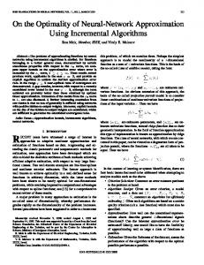
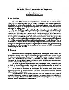
Example 3.8.1. As an example of the above conversion, suppose we are given a CNN which takes as input 13 × 13 grayscale images and outputs to its top fully connected layers 10 different (single pixel) features. We look at each feature separately and show that it may be computed by an extended CBCL NN. Note that CBCL NN’s (extended or not) compute a single global (top gate) output, so we need6 10 of these NN’s to produce these 10 features. We will do the conversion for the first feature. Suppose there are 3 lower layers (before the fully connected part): • each gate of the bottom layer computes 8 convolution-based feature maps (with weight matrices W 1 , . . . , W 8 ) on 3 × 3 patches and squashes each with a logistic function. • each gate of the hidden layer computes a max over a 5 × 5 grid of the bottom layer output and thus handles a 7 × 7 receptive field. • the single “top” gate (of the lower part of the CNN, for one feature) computes a convolution-based feature map (with weight tensor U ) and squashes it with a logistic function; it thus handles a 13 × 13 receptive field. Figure 3.1 illustrates how the size of these receptive fields was determined. Let the over-all input to the CNN be x, the output of the next layer (i.e. input to the hidden layer) be 5

This is a special case of convolution with many weights 0 and others 1. Actually, one could use a portion of a single CBCL NN (with multiple outputs upwards) but technically this would not be a CBCL NN; extended or not, these require a single top gate. 6

34


y, the output of the hidden layer (i.e. input to the top layer) be z, and the output of the top layer w. Then, in the convolution + squashing operations we compute ! X k k yi = σ Wh · [subi (x)]h + B , for k = 1, . . . , 8 and i ∈ [−5, 5] × [−5, 5], h∈H

and  w = σ

 X

Uhj1 · [sub(0,0) (z j )]h + B 00  .

h∈H 00 ,j∈J

Here H = [−1] × [1] (a centred 3 × 3 grid) and H 00 = [−3] × [3] (a centred 7 × 7 grid). In each case the transformation h = (a, b) ∈ [−n] × [n] picks out the pixel which lies a units to the right of the center and b units above the center (a and b may be negative) of whatever image it is acting on. In the case of the top layer computation, there is only one 7 × 7 sub-image of the 13 × 13 global image which gets used. This is the one centred at (0, 0). There is also just one pixel of output (for the first feature, which we have chosen to work with). In the computation of yik we let i range across a central 11 × 11 subimage of x; thus, each of the planes, y 1 , . . . , y 8 , is of size 11 × 11. For consistency with the standard notation (used for weight tensors of a CNN), j1 appears in superscript on U in the above formula. The 1 indicates that we are computing the first feature and the j indicates the plane to which weights will be applied (by the matrix U j1 ). The hidden layer, on the other hand, computes, zik = σ max0 [subi (y k )]h + B 0 , for i ∈ [−3, 3] × [−3, 3], h∈H

where H 0 = [−2, 2] × [−2, 2] (a centred 5 × 5 grid). Remark 3.8.1 (Size of sub-images). Note that subi is not the same in each context in which it is used. The size of the sub-image that it produces varies and is not noted explicitly. It should however be clear from the context. When we see K3 (subi x, t0 ) we know that subi must produce 7 × 7 images because K3 is defined on X3 . Remark 3.8.2 (Variable names). As mentioned, the top layer convolution operation uses z as input, and the hidden layer uses y as input. This is a deviation from the variable names used at the beginning of this section, where y named an intermediate output which still needed to be squashed before being sent on to serve as input for the next layer. Now (to avoid excess notation) these variables denote outputs after squashing.

3.8. EXAMPLE OF CONVOLUTION NEURAL NET TO CBCL CONVERSION

35

Figure 3.1: The three patches of sizes 3 × 3, 5 × 5 and 7 × 7, with their centers shaded. They correspond to the patches used by y, z and w respectively. They are placed with the center of each patch at the corner of the next one to illustrate the maximum receptive field that will be covered (in this example, patch size happens to increase with the layer of the CNN). By labeling the pixels of the patches respectively with coordinates [−1, 1] × [−1, 1], [−2, 2] × [−2, 2] and [−3, 3] × [−3, 3] it is clear that the maximum over-all receptive field can be labeled with [−6, 6] × [−6, −6] (because 1 + 2 + 3 = 6), i.e. it is of size 13 × 13. Similarly, one works out that the lower layer gates handle receptive fields of size 7 × 7 (hidden layer) and 3 × 3 (bottom layer). The bottom and top convolution layers are linear filters followed by squashing functions. In fact, this example is inspired by the lower layers of the NN in Amit [1] (where a discrete thresholding function is used instead of the sigmoid), but can equally well be cast as a CNN example, as we do here. To implement the above CNN with a CBCL NN, we use the following spaces: X0 = 1 × 1 images X1 = 3 × 3 images X2 = X1 X3 = 7 × 7 images X4 = 13 × 13 images X5 = X4 . We start with a simple inner product K0 on X0 (computing the product of single pixel values) and then build up kernels recursively until obtaining K5 (x, t) defined for x, t ∈ X5 with t fixed and x arbitrary. There are no bias terms in this example. The general scheme is as follows:

36


First, there will be 8 kernels derived on X2 = X1 corresponding to the 8 feature vectors on the second layer of the CNN. This is done in two steps: first deriving kernels K11 , . . . , K18 on X1 from K0 by weighted averages (with weights given by W ) and then using the method explained in “Problems” to (respectively) derive kernels K21 = σ(K11 ), . . . , K28 = σ(K18 ) on X2 = X1 from these. Then, we derive 8 kernels on X3 from the previous ones, using a max neural response (with set of transformations [−2, 2] × [−2, 2]). There is no cross-interaction: for each j = 1, . . . , 8 the kernel K3j is derived from K2j . Next, we derive a single kernel K4 on X4 as a sum of 8 different kernels K41 , . . . , K48 , each derived via a weighted average (with weights for the j’th one given by U j1 ). Finally, we use the method in “Problems” to derive a kernel K5 = σ(K4 ) on X5 = X4 from K4 .

3.9

Lifting an abstract neural map

Suppose one has a neural response (i.e. map, in general) N` : X` → F`−1 which maps into some Hilbert space F`−1 of functions on X` and the inner product of F`−1 is then pulled back via N` to obtain a kernel K` on X` : K` (·, ·) = hN` (·), N` (·)iF`−1 . In the CBCL model F`−1 = L2 (T`−1 ). Then N` may in fact be lifted to a map e` : HK → F`−1 N ` so the diagram below commutes. This observation was made in joint work with A. Wibisono for the case F`−1 = HK`−1 . The argument for that case goes through in the general case and is reproduced below. Here Φ` : X` → HK` is the feature map that sends x ∈ X` to K`,x ∈ HK` . e` N -

F`−1

-

HK`

N

Φ`

`

6

X` e` (K`,x ) = N` (x) for each x ∈ X` , then extending by This is accomplished by setting N e` is welllinearity and continuity. The following lemma shows that this construction of N defined. To see this construction more concretely, suppose N` is a max neural response: N` (x)(t) = hK`−1,ht (x) , K`−1,t iHK`−1 ,

3.9. LIFTING AN ABSTRACT NEURAL MAP

37

where ∀t ∈ T`−1 , ht is the element h ∈ H` which maximizes hK`−1,ht (x) , K`−1,t iHK`−1 . Then, e` (K`,x )(t) = hK`−1,h (x) , K`−1,t iH N , ∀t ∈ T`−1 . K`−1 t Lemma 3.9.1 (Fraser, Wibisono). Given N` as above, it follows that m X

ai K`,xi = 0 =⇒

i=1

m X

ai N` (xi ) = 0

i=1

e` on the K`,x ’s by linearity to a map and hence one may extend the basic definition of N e 0 : span{K`,x | x ∈ X` } → F`−1 . N ` e 0 is in fact a linear isometry and hence may be extended by continuity to a Moreover, N ` map e` : HK → F`−1 . N ` Proof. We have m m P P ai K` (xi , x) = 0, ai K`,xi = 0 ⇒ i=1 m P

i=1

⇒

ai hN` (xi ), N` (x)iF`−1 = 0, E ⇒ ai N` (xi ), y = 0, F`−1 E D i=1 m P ai N` (xi ), y = 0, ⇒ i=1 D m P

F`−1

i=1

which implies that

m X

∀x ∈ X` ∀x ∈ X` ∀y ∈ N` (X` ) ∀y ∈ spanN` (X` ),

⊥ ai N` (xi ) ∈ spanN` (X` ) .

i=1

Pm

P Since clearly i=1 ai N` (xi ) lies in the span of N` (X` ), we conclude that m i=1 ai N` (xi ) = 0, e 0 by linearity to a well-defined map as desired. This allows us to extend N ` e 0 : span{K`,x | x ∈ X` } → F`−1 . N ` e 0 is linear and the inner product defined on the pre-Hilbertian space By definition, N ` e 0 of span{K`,x | x ∈ X` } within HK` is the same as that obtained by pullback via N ` e 0 is therefore an isometry. Indeed, given α, β ∈ span{K`,x | x ∈ X` }, we have h·, ·iF`−1 . N ` kα − βk2HK

`

= hα − β, α − βiHK` e 0 (α − β), N e 0 (α − β)iF = hN ` ` `−1 0 0 0 e e e e 0 (β)iF = hN (α) − N (β), N (α) − N =

` e 0 (α) kN `

−

` ` 0 2 e (β)|| N F`−1 , `

`

`−1

38


e 0 takes Cauchy sequences to Cauchy sequences. In particular, if two sequences conso N ` e 0 will also converge and share verge to the same limit in HK` then their images under N ` ∞ a limit. Therefore, given α ∈ HK` we may take any (αn )n=1 ⊂ span{K`,x | x ∈ X` } such e` (α) = limn→∞ N e 0 (n ). that α = limn→∞ αn in HK` , and define N ` In the above proof we also proved the following. e` implies that N` = N e` ◦ Φ` , and hence that the Lemma 3.9.2. Such a definition of N e inner product on HK` is a pullback of that on F`−1 via N` .

3.9.1

e` Injectivity of N

e` is injective (by the last statement in ProposiWe remark that this in fact implies N e` as above, irrespective of whether N` is tion 3.4.3). This occurs once we can define N injective. It is a consequence of the way in which the feature map kills off the degenerate part of a kernel in lifting to the Hilbert space (see the discussion in Section 3.4.1). e` is an isomorphism of Hilbert spaces between HK and N e` (HK ) = Therefore, N ` ` spanN` (X` ), and we have the following commutative diagram. e` N

- F`−1 -

HK`

-

⊂

∼=

spanN` (X` )

3.10

Templates of the first and second kind

Poggio et al sometimes refer to templates of the second kind. We define this notion below. To distinguish it from the notion of templates we have discussed up to now, they use the term templates of the first kind for the latter. Definition 3.10.1 (Templates of the Second Kind). A set of templates of the second kind is a set T` ⊂ HK` . It implies some modifications to the basic framework described so far. Namely, for ` = 2, . . . , d the neural responses are taken to be of the form N` : X` → L2 (T`−1 , ν`−1 ) and the recurrence is K` (x, x0 ) = hN` (x), N` (x0 )iL2 (T`−1 ,ν`−1 ) , where ν`−1 is a measure on T`−1 .

3.10. TEMPLATES OF THE FIRST AND SECOND KIND

39

Remark 3.10.2. To distinguish the two kinds of templates, we will always use calligraphic letters, such as T , for templates of the second kind, and roman letters, such as T for templates of the first kind. Note that both Nmax and Navg can be viewed as neural responses of this type as follows: Nmax (x)(τ ) = maxhK`−1,h(x) , τ iK`−1 h∈H

and X

Navg (x)(τ ) =

µH `−1 (h)hK`−1,h(x) , τ iK`−1

h∈H

where τ ∈ T ⊂ HK`−1 is a template of the second kind and x ∈ X` . This is compatible with the usual definition of these neural responses since in general we have K(y, z) = hKy , Kz iK (see Section 3.4.1).

3.10.1

Using templates of the second kind with linear neural responses

Consider now an arbitrary neural response N : X2 → L2 (T, ν) which satisfies Axiom 3.5.1 and is linear (so the linear base neural response Nbase : X2 → HK1 is well-defined) we can then define N 0 : X2 → L2 (T 0 , ν 0 ), for any set of templates of the second kind, T 0 ⊂ HK1 with measure ν 0 , as follows: N 0 (x)(τ ) = hNbase (x), τ iK1 , ∀τ ∈ T 0 . This is an extension - to templates of the second kind - of the formula in Axiom 3.5.1; that formula says how to evaluate neural responses in terms of base neural responses, in the case of templates of the first kind. In particular, if T 0 = {Φ1 (t) : t ∈ T } and we let ν 0 denote the pushforward of ν via Φ (defined on T 0 by ν 0 (Φ1 (t)) := ν(t), ∀t ∈ T ), then: hN (·), N (·)iL2 (T,ν) = hN 0 (·), N 0 (·)iL2 (T 0 ,ν 0 )

3.10.2

(3.10.1)

Caution regarding templates of the second kind for non-linear neural responses

Suppose N : X2 → L2 (T, ν) satisfying Axiom 3.5.1 is possibly non-linear. We would like to define evaluation of N for templates of the second kind in a compatible manner, i.e., by a formula which reduces to (3.10.1) when N is linear. Specifically, ρT (Nbase )(x2 ) (as a m P functional on T ) should map τ = ai K1,xi ∈ T to i=1 m X i=1

ai hNbase (x2 )(xi ), K1,xi iK1 ,

40


where x1 , . . . , xm ∈ X1 are chosen so K1,x1 , . . . , Km,xm form a basis for HK1 . However this in general will depend on the choice of x1 , . . . , xm ∈ X1 if N is nonlinear and so is not well-defined. Therefore, either one must restrict oneself to using templates of the second kind only with linear neural responses or one must specify a particular maximally independent subset of Φ1 (X1 ), i.e. specify x1 , . . . , xm ∈ X1 such that K1,x1 , . . . , Km,xm form a basis for HK1 (then the above calculation will be well-defined with respect to that subset). Alternatively, if one considers T = Φ1 (T ) for some template set T of the first kind then this issue does not arise; one defines ρT (Nbase )(x2 )(Φ1 (t)) := ρT (Nbase )(x2 )(t) = hNbase (x2 )(t), K1,t iK1 .

3.11

Closer look at the average neural response

We now take a closer look at the CBCL model in the special case of the average neural response.

3.11.1

Skipping a layer

Let N` be an average neural response. It turns out that the composed map e`−1 ◦ · · · ◦ N e1 N` ◦ N is again an average neural response, with the natural transformation set, and that it produces the same kernel on the top layer if one allows templates of the second kind. This is therefore not a true collapsing of the layers within the original CBCL model. It was first observed in joint work of the author with A. Wibisono, and the exposition given here follows that work. One of the main results of this thesis (Proposition 4.5.1) is a strengthening of that initial result (allowing us to choose the templates), which does produce true collapsing within the CBCL model – in fact for arbitrary linear neural responses. We perform the computation for a 3-layer architecture; the general case will then follow by induction. Assume the standard setting and notation, so we have the following diagram. HK3

e3 N

- HK 2 - 6

6

Φ3 X3

N3

Φ2 X2

e2 N

- HK 1 - 6

N2

Φ1 X1

3.11. CLOSER LOOK AT THE AVERAGE NEURAL RESPONSE

41

Let H = {h ◦ h0 | h ∈ H2 , h0 ∈ H3 } (which are transformations from X3 to X1 ) and define H the measure µH on H to be the pushforward measure of µH 2 × µ3 on H2 × H3 under the 0 0 map (h, h ) 7→ h ◦ h . Consider the following diagram e† N

HK3

- HK 1 - 6

6

N†

Φ3

N1 X1

X3

where N† is the average neural response defined by the transformations in H. Given x ∈ X3 , we can compute X 0 e2 ◦ N3 )(x) = N e2 (N K2,h0 (x) µH (h ) 3 h0 ∈H3

=

X

0 e2 (K2,h0 (x) )µH N 3 (h )

h0 ∈H3

=

X

0 N2 (h0 (x))µH 3 (h )

h0 ∈H3

=

X X

H 0 K1,h◦h0 (x) µH 2 (h)µ3 (h )

h0 ∈H3 h∈H2

=

X

K1,g(x) µH (g)

g∈H

= N† (x). We now wish to compare the kernel K3 = N3∗ h·, ·iL2 (T2 ) with the kernel one would obtain via N† , K30 := N†∗ h·, ·iL2 (T1 ) . However, we will at this point need to allow template sets of the second kind: T ⊂ HK . (see Section 3.10). Specifically, we will be comparing kernels derived by the following two architectures: Architecture 1. Three-layers: i.e. spaces X1 , X2 , X3 , transformation sets (H1 , µ1 ) and (H2 , µ2 ), initial kernel K1 , template sets of the second kind (T1 , ν1 ), (T2 , ν2 ), average neural responses N2 , N3 , and derived kernels K2 , K3 .

42


Architecture 2. Two-layers: space X1 as the bottom layer and X3 as the top layer (no hidden layer). The transformation set is given by H = {h2 ◦ h3 | h2 ∈ H2 , h3 ∈ H3 }, and the measure µ on H is given by the pushforward measure from H2 × H3 via the map (h2 , h3 ) 7→ h2 ◦ h3 . The initial kernel on X1 is K1 . The template set is T = F (T2 ) ⊂ HK1 , where F : HK2 → HK1 is given by F (τ ) =

X τ 0 ∈T

e2 (τ )(τ 0 ) τ 0 ν1 (τ 0 ), N

(3.11.1)

1

with the measure ν = F∗ ν2 . The neural response N† : X3 → L2ν (T ) is the average neural response X N† (x)(τ ) = hK1,g(x) , τ iHK1 µ(g), g∈H

for x ∈ X3 , τ ∈ T and the derived kernel K† : X3 × X3 → R is given by K† (x, x0 ) = hN† (x), N† (x0 )iL2ν (T ) , for x, x0 ∈ X3 . Remark 3.11.1. Note that T = F (T2 ) ⊂ spanT1 .

We now prove:

Proposition 3.11.2 (Fraser and Wibisono). For any x ∈ X3 and τ ∈ T2 , we have N3 (x)(τ ) = N† (x)(F (τ )), and therefore, K3 (x, x0 ) = K† (x, x0 )

for all x, x ∈ X3 .

3.12. UNDERLYING NEURAL NETWORK

43

Proof. Let x ∈ X3 and τ ∈ T2 . We compute X hK2,h3 (x) , τ iHK2 µ3 (h3 ) N3 (x)(τ ) =

(3.11.1)

h3 ∈H3

=

X

e2 (τ )iL2 hN2 (h3 (x)), N ν

1

(T1 )

µ3 (h3 )

(3.11.2)

h3 ∈H3

=

X X h3 ∈H3

=

τ 0 ∈T

e2 (τ )(τ 0 ) ν1 (τ 0 ) µ3 (h3 ) N2 (h3 (x))(τ 0 ) N

(3.11.3)

1

X X X

e2 (τ )(τ 0 ) µ2 (h2 ) ν1 (τ 0 ) µ3 (h3 ) hK1,h2 ◦h3 (x) , τ 0 iHK1 N

h3 ∈H3 τ 0 ∈T1 h2 ∈H2

=

X X

e2 (τ )(τ 0 ) µ(g) ν1 (τ 0 ) hK1,g(x) , τ 0 iHK1 N

(3.11.4)

g∈H τ 0 ∈T1

=

E X XD e2 (τ )(τ 0 ) τ 0 ν1 (τ 0 ) K1,g(x) , N τ 0 ∈T1

g∈H

|

{z

=F (τ )

HK1

µ(g)

(3.11.5)

}

= N† (x)(F (τ )).

(3.11.6)

Therefore, for any x, x0 ∈ X3 , K3 (x, x0 ) = hN3 (x), N3 (x0 )iL2ν (T2 ) 2 X = N3 (x)(τ ) N3 (x0 )(τ ) ν2 (τ ) τ ∈T2

=

X

N† (x)(F (τ )) N† (x0 )(F (τ )) ν2 (τ )

τ ∈T2

=

X

N† (x)(b τ ) N† (x0 )(b τ ) ν(b τ)

τb∈T

= hN† (x), N† (x0 )iL2ν (T ) = K† (x, x0 ).

3.12

Underlying neural network

The framework just described can be computed by the neural network defined in the Figures below. We refer to this NN model as the CBCL model or extended CBCL model - the distinction will be made clear below. Together, Figure 3.2 and Figure 3.3 show the recursive step of the computation, namely, how K` is obtained from K`−1 . Figure 3.3 is a close-up of the workings of a t-filter, which

44


Figure 3.2: The neural network computing K` (x, y), for x, y ∈ X` . Each rounded rectangle represents a ti -filter of the kind depicted in the Figure 3.3. More details are given in Remark 3.12.1. is a subnetwork of the neural network in Figure 3.2. The entire neural network is obtained by substituting a network analogous to that of Figure 3.2 (which computed K` ) to perform each of the calculations of K`−1 appearing in Figure 3.3 and so on... until reaching K1 which is assumed to be computed atomically (either by a single computational gate, or a fixed network with all known components). Remark 3.12.1 (on the Figures). We have used rounded rectangles to represent tfilters, sharp-cornered rectangles, i.e. boxes, to represent nodes computing a kernel (K` or K`−1 ) and finally, ovals/circles for all other computational nodes. In Figure 3.2, the gate marked IP computes the inner product in L2 (T`−1 , ν`−1 ): ((z1 , . . . , zr ), (w1 , . . . , wr )) 7→

r X

zi wi ν(ti ),

i=1

where T`−1 = {t1 , . . . , tr ). In Figure 3.3, the gate marked µ-sum over all h is a weighted average. Supposing H`−1 = {h1 , . . . , hN }, this gate computes (z1 , . . . , zN ) 7→

N X

µH `−1 (hi )(zi ).

i=1

If the t-filter were based on a different pooling, namely the max operation, then we would


45

Figure 3.3: A t-filter, as used in the above neural network; this one pools by weighted average, pooling by max would be analogous, or alternatively any other neural response could be used. More details are given in Remark 3.12.1. Here we assume t ∈ X`−1 is a template and µ is the measure on H = {h1 , . . . , hN } ⊂ Maps(X2 , X1 ). For each i ∈ [N ] the input x ∈ X` is converted into hi (x) ∈ X`−1 before being input into a box computing K`−1 (t, ). This box is of the same type as that of Figure 3.2 which computed K` (·, ·). Note: a t-filter is thus defined by the pooling function (with H) and the kernel K`−1 . have, instead of this gate, one marked max over all h, which computes (z1 , . . . , zN ) 7→ max zi . i∈[N ]

In order to implement an arbitrary neural response, the subnetworks which compute K`−1 (h(x), ·) in Figure 3.3 would be possibly indexed by some set other than H. See Section 3.12.2. Definition 3.12.2 (Extended CBCL model vs. CBCL model). These are distinguished by two aspects. 1. The extended CBCL model allows ti - and tj -filters to be different, i.e. to use different kernels K`−1 and pooling functions (i.e. neural responses) for i 6= j. The CBCL model requires that all filters on a given level use the same kernel. In either model, a given ti -filter (which appears twice) must be the same in both its occurrences.

46

CHAPTER 3. CBCL MODEL 2. The extended CBCL model allows arbitrary neural responses satisfying Axiom 3.5.1. The CBCL model restricts the neural responses to be either N max or N avg .

3.12.1

Convolution Neural Networks

The lower layers of a convolution neural network alternate pooling by weighted average and sub-sampling (which amounts to pooling with some weights zero) or sometimes max’ing. The final, upper layers are fully connected, using linear neural responses. The discussion in Section 3.7 shows that a convolution neural network may be viewed as a special case of an extended CBCL network.

3.12.2

General t-filters

Suppose t ∈ X`−1 is a template. Then a t-filter of the CBCL or extended CBCL model (there is no difference as far as individual t-filters are concerned) computes, for any x ∈ X` , hNbase (x)(t), K`−1,t iHK`−1 where Nbase : X` → Maps(X`−1 → HK`−1 ) is a particular base neural response and K`−1 a kernel on X`−1 , both of which have been fixed in advance to define that t-filter. Standard t-filters – those with N avg or N max – make use of a transformation set H to index computations of the type K`−1 (h(x), t) which are then pooled. A similar principle can be used to construct a general t-filter, since HK`−1 is finite-dimensional (X`−1 is finite in all NN applications). Let x1 , . . . , xn ∈ X`−1 be such that K`−1,x1 , . . . , K`−1,xn form a basis for HK`−1 . Then to each x ∈ X` we may associate a1 (x), . . . , an (x) such that X Nbase (x)(t) = ai (x)K`−1,xi . i∈[n]

The ai (x) of course depend on t as well, but this is fixed for the given filter. Define n computational gates, where the i’th one computes ai (x)K`−1 (xi , t). Pool the outputs of these n gates at a higher level gate by summing them. This produces X X ai (x)K`−1 (xi , t) = ai (x)hK`−1,xi , K`−1,t iHK`−1 i∈[n]

i∈[n]

= hNbase (x)(t), K`−1,t iHK`−1 which is exactly what this t-filter should compute. Thus every Nbase – not just N avg or N max – is in fact a pooling.


47

Caveat. This is not meant as a practical solution. Rather, its purpose is to allow us to formally define a class of NN’s which correspond to the architectures of the (extended) CBCL model. The algebraic complexity of computing the functions ai (·) (and also hi (·) in the definition below) must be addressed before comparing instances of this class. Note that computing h(x) is usually free in nature, as neurons are hardwired to collect data from the appropriate sub-patch of the visual field. Definition 3.12.3 (General t-filter). We define a general t-filter as an NN whose top (global output) gate pools by sum or by max the outputs of n lower gates, each of which computes ai (x)K`−1 (hi (x), t) for an i ∈ [n], where ∀x ∈ X` , ∀i ∈ [n] ai (x) ∈ R and hi (x) ∈ X`−1 . The computation above shows that by allowing Figure 3.3 to be a general t-filter, the resulting class of extended CBCL NN’s is broad enough to include an instance for each extended CBCL architecture. In other words, for each mathematicval hierarchy in the framework there is an NN which computes it. Definition 3.12.4. Given an NN of the CBCL or extended CBCL model, we refer to the gates which appear explicitly in Figure 3.2 together with those in Figure 3.3 as forming a stage. One stage thus corresponds to a transition between spaces X` and X`−1 in the mathematical framework. Therefore a d − 1-stage NN corresponds to a d-layer architecture of the framework.

48


Chapter 4

Decomposing and Simplifying the Hierarchy We begin, in Section 4.1, by stating four Propositions which show the inter-relation between design aspects of neural networks used for deriving reproducing kernels. Specifically we look at how choice of neural response, choice of transformations and choice of templates are related. These results also reveal on a Hilbert space level the mechanics of this kernel construction and show that there is an inherent formal linearity in the kernels thus obtained. This observation allows us in Section 4.5 to collapse hierarchies where we have sufficient freedom of choice in the mentioned design aspects. For such hierarchies, and purely in terms of the class of kernels which the underlying NN’s compute, shallow networks are equivalent to deep ones. In nature such freedom of choice is most likely not present. Even for abstract neural networks, learning considerations may well restrict this freedom.

4.1

Initial structural results

The four propositions below all assume the same two-layer CBCL architecture, with some additional assumptions. We will however, allow neural responses other than N avg and N max when indicated. We now describe the assumptions and fix the notation.

4.1.1

Assumed architecture

Start with a two-layer CBCL architecture (see Definition 3.3.1): spaces X1 and X2 , a reproducing kernel K1 on X1 , a finite set of templates T1 = {t1 , . . . , tm } ⊂ X1 equipped with measure ν1 and a neural response S : X2 → L2 (T1 , ν1 ), 49

50

CHAPTER 4. DECOMPOSING AND SIMPLIFYING

such that the reproducing kernel K2 on X2 is derived via S (as given by Equation 3.2.1): K2 (·, ·) := hS(·), S(·)iL2 (T1 ,ν1 ) . We assume that S satisfies Axiom 3.5.1 but for the time being, do not restrict S further. Note that convolution networks are special cases of extended CBCL networks and we will see how these may be handled in Section 4.6. We assume further that T1 = {Φ1 (ti ) : i ∈ [m]} is linearly independent and for each i ∈ [m], let τi = Φ1 (ti ). We let n = dim HK2 , so n ≤ m ≤ dim HK1 1 . Additional Notation: We use πY to denote projection onto the linear span of Y , when Y is a subset of a Hilbert space.

4.1.2

Propositions

First, we address replacing an arbitrary neural response by a linear one (or several linear ones - see the Corollary). Proposition 4.1.1. Assume the architecture specified in Section 4.1.1. There exists a linear neural response S 0 : X2 → L2 (T1 , ν1 ) such that K2 can be derived via S 0 : K2 (·, ·) := hS 0 (·), S 0 (·)iL2 (T1 ,ν1 ) . 0 (x), tiHK1 agree for all x ∈ X2 and t ∈ T1 . In particular, hSbase (x), tiHK1 and hSbase

Corollary 4.1.2. Given an arbitrary neural response S : X2 → L2 (T ) satisfying Axiom 3.5.1, and a partitioning of T as T = T1 ∪ . . . ∪ Tr where each Ti = Φ1 (Ti ) is a linearly independent set in HK1 , the derived kernel K2 induced by S on X2 can be written as K2 (·, ·) = K 1 (·, ·) + . . . + K r (·, ·) where each K i is a kernel on X2 induced by a linear base neural response i Nbase : X2 → HK1 .

Proof of the Corollary. This is a consequence of the fact that L2 (T, ν) can be expressed as a direct sum L2 (T, ν) = L2 (T1 , ν1 ) ⊕ · · · ⊕ L2 (Tr , νr ), where νi is the restriction of the measure ν to the subset Ti ⊂ T . Thus, K2 (x, x0 ) = hS(x), S(x0 )iL2 (T ) = hπY1 ◦ S(x), πY1 ◦ S(x0 )iL2 (T1 ) + · · · + hπYr ◦ S(x), πYr ◦ S(x0 )iL2 (Tr ) 1

If m = dim HK1 then πT1 is the identity, so πT1 ◦ Sbase = Sbase .

4.1. INITIAL STRUCTURAL RESULTS

51

for any x, x0 ∈ X2 , where Yi denotes the elements of L2 (T, ν) which are zero on t ∈ T \ Ti . We then obtain the desired fact by applying Proposition 4.1.1 to each of the neural responses πTi ◦ S : X2 → L2 (Ti ), i = 1, . . . , r. Before proceeding with the next Proposition, we clarify one of the hypotheses we will be using. Lemma 4.1.3. Suppose S : X → F(T ), a Hilbert space, and K2 (·, ·) = S ∗ h·, ·iF (T ) . Let Φ2 : X2 → HK2 be the associated feature map. Then k X

ai Φ2 (xi ) = 0 ⇔

i=1

k X

ai S(xi ) = 0

i=1

holds for any k ∈ N, a1 , . . . , ak ∈ R, x1 , . . . , xk ∈ X2 . Proof. X

X ai K2,xi = 0 ⇒ (∀y ∈ X2 )h ai K2,xi , K2,y iHK2 = 0 X ⇒ (∀y ∈ X2 ) ai K2 (xi , y) = 0 X ⇒ (∀y ∈ X2 )h ai S(xi ), S(y)iF (T ) = 0 X ai S(xi ), wi = 0 ⇒ (∀w ∈ spanS(X2 ))h X ⇒ ai S(xi ) = 0

P since spanS(X2 ) is a Hilbert space to which ai S(xi ) belongs. The reverse implications are mostly trivial; the top one uses the fact that HK2 = span{K2,y : y ∈ X2 }. We now show that a neural response can be changed on points x1 , . . . , xk ∈ X2 for which {Φ2 (x1 ), . . . , Φ2 (xk )} are linearly independent, while still retaining the same derived kernel K2 (on those points) provided we have the freedom to change the templates to arbitrary templates of the second kind. Proposition 4.1.4. Assume the architecture specified in Section 4.1.1. By the pevious proposition, assume without loss of generality that Sbase is linear. Let Nbase : X2 → HK1 be any specific linear base neural response. Suppose x1 , . . . , xk ∈ X2 such that S(x1 ), . . . , S(xk ) ∈ L2ν (T1 ) are linearly independent. Then Nbase (x1 ), . . . , Nbase (xk ) ∈ HK1

52


are linearly independent if and only if there exists a set of templates of the second kind, T ⊂ HK1 , contained in the span of the Nbase (xi ), and a measure ν on T such that: K2 (xi , xj ) = hN (xi ), N (xj )iL2ν (T ) , ∀i, j ∈ [k]

(4.1.1)

where N = ρT (Nbase ) is the neural response into L2ν (T ) induced by Nbase . Moreover, if k is maximal, i.e. k = dim HK2 , then such T , when it exists, is unique. That (4.1.2) implies the N (xi ) are linearly independent is an immediate consequence of Lemma 4.1.3. Using N (x) = πT ◦ Nbase (x), ∀x ∈ X2 , this then implies the Nbase (xi ) are linearly independent. The other direction, i.e. the existence of suitable T , ν, remains to be proved, as does uniqueness. Remark 4.1.5. More generally, by Lemma 4.1.3, having K2 (x, x0 ) = hN (x), N (x0 )iL2ν (T1 ) for all x, x0 ∈ U for some subset U ⊂ X2 , implies the linear dependencies induced by S within U coincide with those induced by N . We will return to this discussion in Section 4.2.3. Remark 4.1.6. The non-existence or uniqueness of templates of the second kind making (4.1.2) hold applies to templates of either first or second kind, since h·, ·iL2 (T,ν) = h·, ·iL2 (T 0 ,ν 0 ) for T 0 = {Φ1 (t) : t ∈ T } and ν 0 = (Φ1 )∗ ν; see Section 3.10 and in particular equation (3.10.1) for details. We emphasize, as a Corollary, a particular case of the final statement of the Proposition. Corollary 4.1.7. In particular, in the previous Proposition, if we are interested in obtaining a given weighted average, i.e. X avg Nbase (x) = Nbase (x) = µ(h)K1,h(x) , ∀x ∈ {x1 , . . . , xk } ⊂ X2 h∈H

(with fixed choice of transformation set H and measure µ on H) then (4.1.2) is possible if and only if x1 , . . . , xk ∈ X2 are such that, X X µ(h)K1,h(x1 ) , . . . , µ(h)K1,h(xk ) ∈ HK1 h∈H

h∈H

are linearly independent. See Section 4.2.3 regarding extension of (4.1.2) to all x, x0 ∈ X2 (not just x, x0 ∈ {x1 , . . . , xk } ⊂ X2 ). Somewhat of a converse to the previous Proposition also holds, allowing us to choose the templates but then forcing the neural response.

4.2. PRELIMINARIES

53

Proposition 4.1.8. Assume the architecture specified in Section 4.1.1. By the Proposition 4.1.1, assume without loss of generality that Sbase is linear. Let T = {si : i ∈ [m]} ⊂ X1 be any specific template set such that Φ1 (s1 ), . . . , Φ1 (sm ) are linearly independent. Suppose x1 , . . . , xn ∈ X2 such that S(x1 ), . . . , S(xn ) ∈ L2ν (T1 ) are linearly independent. Then there exists a linear base neural response Nbase into the span of the Φ1 (si ) such that K2 (xi , xj ) = hN (xi ), N (xj )iL2ν (T ) , ∀i, j ∈ [k]

(4.1.2)

where N = ρT (Nbase ) is the neural response into L2ν (T ) induced by Nbase . Moreover, if k is maximal, i.e. k = n = dim HK2 , then this Nbase is unique. Finally, we show that linear neural responses can always be replaced by weighted averages when H, µ are not fixed in advance. We do this by constructing H, µ which make the conditions of the previous Corollary hold. Proposition 4.1.9. Assume the architecture specified in Section 4.1.1. Suppose m < dim HK1 or there exists y ∈ X1 such that K1,y = 0. Also suppose X2 is finite (as it would be in all practical applications)2 . Then there exists a finite transformation set H ⊂ Maps(X2 → X1 ) and measure µ on H such that the weighted average N avg that H, µ define into L2ν (T1 ) induces a derived kernel that coincides exactly with K2 , the kernel induced by S. In other words, S can be replaced by a weighted average.

4.2

Preliminaries

Before proving the Propositions, we develop some tools. We first observe a general fact about linear independent vectors and inner products.

4.2.1

Change of bases

Lemma 4.2.1. Suppose we are given two sets of k linearly independent vectors: σ1 , . . . , σk and η1 , . . . , ηk in an n-dimensional real Hilbert space with inner product h·, ·i and a basis τ1 , . . . , τm . Then there exists a new basis τ˜1 , . . . , τ˜m such that hσi , τj i = hηi , τ˜j i for all i, j. 2 In fact, as long as there are only finitely many vectors N (x2 ) such that x2 ∈ X2 the same construction can be made to work.

54


Proof. First, assume that k = m, by completing the linearly independent sets to bases (in arbitrary fashion) . Fix j ∈ [m], and for each i ∈ [m] let ci = hσi , τj iK1 . Then Hi := {v : hηi , vi = ci } is an affine hyperplane orthogonal to N (xi ). Specifically, Hi =

ci ηi + span[ηi ]⊥ . ||ηi ||2K1

It can then be shown by induction that

n T

Hi is nonempty. Indeed if the intersection

i=1 k T

Hi is nonempty for some k < m then it is of the form

i=1

w + span[η1 , . . . , ηk ]⊥ and so cannot be parallel to Hk+1 since this would imply ηk+1 ∈ span[η1 , . . . , ηk ]. Therefore

k+1 T

Hi 6= ∅ and by induction,

i=1

m T

Hi 6= ∅. Let τ˜j be an element of this intersection.

i=1

By construction, ∀i ∈ [m], hσi , τj i = hηi , τ˜j i. This P may now be repeated toPconstruct a τ˜j for each j ∈ [m]. P Any linear dependence a τ ˜ = 0 would imply hσ , a τ i = 0 for all i, and hence j j i j j j j j aj τj = 0 because the σi are a basis for the span of τ1 , . . . , τm . Thus the linear independence of the τj forces that of the τ˜j .

4.2.2

Rank

Definition 4.2.2. We define the rank of a neural response as rank (Nbase ) := max dim span(ρT (Nbase )(X2 )) where the maximum is taken over all possible template sets T ⊂ HK1 . Because the elements of ρT (Nbase )(X2 ) are functions on T , rank is bounded above by |X1 | and may in general achieve this. For linear neural responses, however, the functions in ρT (Nbase )(X2 ) are restrictions of elements of HK1 so rank cannot exceed dim HK1 .

4.2. PRELIMINARIES

55

Given finite subsets Y1 ⊂ X1 and Y2 ⊂ X2 , the values of Nbase (y2 )(y1 ) for y1 ∈ Y1 , y2 ∈ Y2 are elements of HK1 and so give rise to functions on Y1 . Let MY1 ,Y2 be the matrix of these values. (MY1 ,Y2 )ij = Nbase (y2 )j (y1 )i (y1 )i , ∀i ∈ [|Y1 |], j ∈ [|Y2 |], where (y1 )i is the i’th element of Y1 and (y2 )j is the j’th element of Y2 . Then the rank of Nbase is just the maximal rank of MY1 ,Y2 over all possible choices of finite subsets Y1 , Y2 .

4.2.3

Formal linear dependencies

Rank is part of a more general phenomemon. We observe that any neural response, as a map from a set X2 to a Hilbert space F(T1 ) induces linear dependencies3 in the set X2 in a formal way. Suppose K2 = N ∗ h·, ·i. Then whenever there are r ∈ N, a1 , . . . , ar ∈ r P R, x1 , . . . , xr ∈ X2 such that ai N (xi ) = 0 we declare the formal linear dependency r P

i=0

ai xi = 0 in the set X2 . Rank is then the maximal cardinality of a set {x1 , . . . , xk } ⊂ X2

i=0

with no nontrivial formal linear dependencies. r r P P Note that ai N (xi ) = 0 if and only if ai K2,xi = 0, by Lemma 4.1.3. Thus, as i=0

i=0

observed in Remark 4.1.5, a necessary condition for a kernel K2 to be derived by the neural response N is that the K2,x satisfy the same linear dependencies as those formally induced among the x ∈ X2 by N . Moroever, if we let x1 , . . . , xn ∈ X2 be such that the K2,xi form a basis for HK2 then the Gram matrix of the K2,xi in the derived Hilbert space HK2 must coincide with the Gram matrix of the N (xi ) w.r.t the inner product in F(T1 ) (this is just a statement of the definition of derived kernel). Conversely, both of these conditions together imply the kernel is derived by N . We have, Lemma 4.2.3. Suppose that two neural responses, N and S, map X2 into F(T ) and F(T 0 ) respectively. Then, the kernels derived via N and S coincide, i.e., hN (x), N (x0 )iF (T ) = hS(x), S(x0 )iF (T 0 ) , ∀x, x0 ∈ X2 if and only if N and S induce the same formal linear dependencies in X2 and Nbase (xi ) = Sbase (xi ), ∀i ∈ [n] for some (hence any) x1 , . . . , xn ∈ X2 such that K2,xi form a basis for HK2 . 3

A motivation of the so-called “kernel trick” is to establish a weaker version of a vector space structure on the space of objects of interest. In fact, it establishes formal linear dependencies as just described, and moreover, a weaker form of an inner product: the derived reproducing kernel.

56


This means that when formal linear dependencies coincide we are able to concern ourselves only with the values of neural responses at elements x1 , . . . , xn such that K2,xi form a basis for HK2 (the formal linear dependencies will take care of all other x ∈ X2 ). On the other hand, when formal linear dependencies do not coincide there is no hope of deriving the same kernel via the two neural responses.

4.2.4

Convenient view of L2 (T ) for finite T

Recall that when a neural response N : X2 → L2 (T ) satisfying Axiom 3.5.1 is linear, we have N (x2 )(t) = hNbase (x2 ), K1,t iHK1 for all x2 ∈ X2 and t ∈ T ⊂ X1 (assuming the usual two-layer notation). Thus, while we pull back the inner product from L2 (T ) (to obtain K2 ), the elements of N (x2 ) are functions on T and are actually obtained by restriction of functions in HK1 to T . They thus correspond to functions in HK1 which are zero on the orthogonal complement of T = Φ1 (T ). Specifically, N (x2 )(t) = hπT ◦ Nbase (x2 ), K1,t iK1 . To make the proofs of the Propositions simpler, we will therefore work within HK1 , using its vector space structure (as a space of functions), and define a non-standard inner product in this vector space which we can pull-back to achieve the same effect obtained by that of L2 (T ). Remark 4.2.4. Warning: We will now have two inner products on the vector space HK1 : one standard, the other not. We will use the notation πT and ⊥ exclusively to mean projection and orthogonal complement according to the standard inner product of HK1 . Suppose we have a finite template set (of second kind) T = {τ1 , . . . , τm } ⊂ HK1 , whose elements are linearly independent. Or if we start with a set of usual templates T ⊂ X1 , then define T = {K1,t : t ∈ T } ⊂ HK1 . Let ν be a total measure on T . Define a non-standard inner product on HK1 by: hu, vi(T ,ν) :=

m X hu, τi iK1 hv, τi iK1 ν(τi ) + hu0 , v 0 iK1 , i=1

u0 , v 0

where are the projections of u, v respectively in span(T )⊥ . This gives the usual inner product on span(T )⊥ but a non-standard one on span(T ). Clearly h·, ·i(T ,ν) is a symmetric bilinear form and it is nondegenerate because only the zero vector v = 0 can belong to span(T ) and at the same time have hu, τi iK1 = 0 for all τi ∈ T . The key property of this inner product is the following. Lemma 4.2.5. Let Nbase be a linear base neural response and N = ρT (Nbase ) the associated neural response into L2ν (T ). Then we have hN (·), N (·)iL2ν (T ) = hπT ◦ Nbase (·), πT ◦ Nbase (·)iT ,ν

(4.2.1)

4.3. PROOF OF THE PROPOSITIONS

57

where πT denotes projection onto the span of T . Proof. Indeed, for x2 , x02 ∈ X2 : hN (x2 ), N (x02 )iL2ν (T ) =

m X

N (x2 )(τi ) · N (x02 )(τi )ν(τi )

i=0

=

m X

hNbase (x2 ), τi iK1 · hNbase (x02 ), τi iK1 ν(τi )

i=0

= hπT ◦ Nbase (x2 ), πT ◦ Nbase (x02 )iT ,ν because πT ◦ Nbase (x2 ) as a linear functional takes on the same values as Nbase (x2 ) on the elements of span(T ) but is zero on their orthogonal complement (i.e. as a vector it belongs to span(T ) ). Note that to each N (x2 ) ∈ L2ν (T ) we have associated πT ◦ Nbase (x2 ) ∈ HK1 .

4.3

Proof of the Propositions

Remark 4.3.1. Let dim HK2 = n. Recall that if K2 is obtained as a pullback via N of an inner product h·, ·iF in a Hilbert space F, then we may lift N to an injective linear e : HK → F (see Section 3.9.1) whose image is the closure of the span of isometry N 2 N (X2 ). This allows us to conclude that N (X2 ) spans an n-dimensional subspace of F (it is closed because finite-dimensional). In our setting, using (4.2.1), this implies that both N (X2 ) ⊂ L2ν1 (T1 ) and πT ◦ Nbase (X2 ) ⊂ HK1 span subspaces of dimension n. Proof of Proposition 4.1.1. Let x1 , . . . , xn ∈ X2 such that Φ2 (x1 ), . . . , Φ2 (xn ) are linearly independent in HK2 . Now, for each i, consider Sbase (xi ) ∈ Maps(X1 → HK1 ). As described in Section 3.10.2, it can be evaluated at each τj ∈ T1 . Since the τj are linearly independent, there exists a linear functional on HK1 which agrees with S(xi ) on T . Let Fi ∈ HK1 be the Riesz representative of this functional. 0 Now let Sbase be the map 0 Sbase : X2 → HK1 defined by 0 Sbase (xi ) := Fi , for each i = 1, . . . , n,

and extended to all of X2 using the formal linear dependencies already induced in X2 (by S). This is a linear base neural response. And, its values on the τj ∈ T1 agree with those of S, therefore, the induced neural response S 0 : X2 → L2 (T1 , ν1 )

58


defines the same derived kernel on X2 as that defined by S. We now prove the Proposition regarding a specific linear neural response Nbase . Proof of Proposition 4.1.4. By the preceding argument we may, without loss of generality, assume that Sbase is linear. Suppose we are given elements x1 , . . . , xn ∈ X2 such that πT1 ◦ Sbase (x1 ), . . . , πT1 ◦ Sbase (xk ) and πT1 ◦ Nbase (x1 ), . . . , πT1 ◦ Nbase (xk ) are both are linearly independent in HK1 . See Remark 4.2.4 regarding the notation πT1 . By Lemma 4.2.1 there exist linearly independent τ˜1 , . . . , τ˜m ∈ HK1 such that (∀i ∈ [n])(∀j ∈ [m]), hπT1 ◦ Sbase (xi ), τj iK1 = hπT1 ◦ Nbase (xi ), τ˜j iK1 . This implies (∀i ∈ [n])(∀j ∈ [m]), hπT1 ◦ Sbase (xi ), πT1 ◦ Sbase (xj )iT1 ,ν1 = hπT1 ◦ Nbase (xi ), πT1 ◦ Nbase (xj )iT ,ν

(4.3.1)

where T = τ˜1 , . . . , τ˜m and ν(˜ τi ) = ν1 (τi ). Given T and ν as above define N = ρT (Nbase ) : X2 → L2ν (T ), the neural response into L2ν (T ) induced by Nbase . We have: K2 (xi , xj ) = S ∗ hxi , xj iL2ν

1

(T1 )

= hS(xi ), S(xj )iL2ν

1

(T1 )

= hπT1 ◦ Sbase (xi ), πT1 ◦ Sbase (xj )iT1 ,ν1 in HK1 = hπT1 ◦ Nbase (xi ), πT1 ◦ Nbase (xj )iT ,ν in HK1 by (4.3.1) = hN (xi ), N (xj )iL2ν (T ) = N ∗ hxi , xj iL2ν (T ) . The final statement of the Proposition follows from Lemma 4.2.3. Remark 4.3.2. In the above proof, if Nbase and Sbase induce the same formal linear dependencies in X2 then so do πT1 ◦ Nbase and πT1 ◦ Sbase so K2 (x, x0 ) and N ∗ hx, x0 iL2ν (T ) coincide for all x, x0 ∈ X2 (extending by linearity the statement proven above for the xi ).

4.3. PROOF OF THE PROPOSITIONS

59

Proof of Proposition 4.1.8. The argument is essentially the same as in the previous proof, except that we use Lemma 4.2.1 instead to get linearly independent τ˜1 , . . . , τñ ∈ HK1 such that (∀i ∈ [n])(∀j ∈ [m]), hπT1 ◦ Sbase (xi ), τj iK1 = hΦ1 (sj ), τ˜i iK1 and then set Nbase (xi ) = τ˜i for each i ∈ [n]. We now prove the final Proposition. Proof of Proposition 4.1.9. We do so by exhibiting a suitable set of transformations H with measure µ. There will be |X2 |d2 transformations, assuming X2 is finite 4 . As before, let T1 = Φ1 (T1 ) and for each i ∈ [m] let τi = Φ1 (ti ). Let y1 , . . . , yd ⊂ X1 be such that K1,y1 , . . . , K1,yd form a basis for HK1 and suppose there is y ∈ X1 such that K1,y is orthogonal to all τi , i ∈ [m]. Such y trivially exists if there is some y with K1,y = 0 and may exist if m < d = dim HK1 . If no such y exists, then at least m < d implies we can find a nontrivial linear comd P bination θ = bi K1,yi which is orthogonal to the span of the τi (because they span an i=1

m-dimensional subspace of the d-dimensional space HK1 ). We will return to this case later, and first deal with the simpler case where a single y exists as described. From now on, write K for K1 to simplify the reading. Let x1 , . . . , xn ∈ X2 be such that πT1 ◦ Sbase (x1 ), . . . , πT1 ◦ Sbase (xn ) are linearly independent. For each j ∈ [d] and for each x, x0 ∈ X2 , let hxj (x0 )

=

yj y

if x = x0 , otherwise.

This makes each hxj into an element of Maps(X2 → X1 ). Now let H = {hxj : j ∈ [d], x ∈ X2 }. It remains to define a measure µ on H. Because the yj were chosen so that Kyj form a basis for HK1 ,P it follows that for each x ∈ X2 , there exist unique coefficients aj (x) such that Sbase (x) = j aj (x)Kyj . For each x ∈ X2 , j ∈ [d] set µ(hxj ) := aj (x). 4 Or, if X2 is infinite but there are only finitely many different vectors N (x2 ) for x2 ∈ X2 , say k of them, then one could alter the proof so that kd or kd2 transformations would suffice.

60


avg Now let Nbase be the (base) weighted average neural response into HK1 . For arbitrary x ∈ X2 , we have avg Nbase (x) =

X X

aj (z)Khzj (x)

j∈[d] z∈X2

=

X

aj (x)Khxj (x) +

X

aj (z)Khzj (x)

j∈[d] z∈X2 z6=x

j∈[d]

=

X X

aj (x)Kyj + R(x)Ky

j∈[d]

= Sbase (x) + R(x)Ky ,

where R(x) =

P P

aj (z) depends only on x. j∈[d] z∈X2 z6=x avg Note that πT1 ◦ Nbase (x) = πT1 ◦ Sbase (x) for each x ∈ X2 so the base neural responses avg have the same associated neural response into T1 . Here we are exploiting Sbase and Nbase the fact that m < d = dim HK1 so base neural responses are not unique (see Proposition 3.5.7). The derived kernel for the given weighted average therefore coincides with K2 . We now address the more complicated case where no single y existed as described, but d P where one does have some nontrivial θ = b` Ky` orthogonal to all τi for i ∈ [m]. We `=1

also require that d X

b` = 1.

`=1

Then construct a set of transformations as above for each ` = 1, . . . , d: H` := {hxj [`] : j ∈ [d], x ∈ X2 }, that are exactly the same as the hxj except that y` should be used instead of y in the case x 6= x0 : hxj [`](x0 ) = y` . Let H 0 =

d S

H` and define a measure ν on H 0 by

`=1

ν(hxj [`]) = b` · µ(hxj ) = b` aj (x)

4.4. EXAMPLES

61

Then for arbitrary x ∈ X2 , we have

avg Nbase (xi )

d X

=

b`

d X

aj (z)Khzj (x)

j∈[d] z∈X2

`=1

=

X X

b` [Sbase (x) + R(x)Ky` ]

`=1

= Sbase (x) + R(x)θ and the rest of the argument is the same.

4.4

Examples

Example 4.4.1. Consider an alphabet Σ = {a, b, c} of 3 letters. Let X1 = T1 = Σ

(4.4.1)

2

X2 = Σ .

(4.4.2)

Let K1 be a kernel on X1 given by the matrix: 

1   M =  q0

0 1 3 4

1 2

q

3 4

1 2

  . 

1

Let S be the max neural response S : X2 → L2 (T1 ) where T1 = {Ka , Kb , Kc } and ν1 is the empirical, i.e. uniform, measure on T1 - from now on when no measure is specified it will be assumed to be uniform. Let K2 be the derived kernel, K2 (·, ·) = S ∗ h·, ·iL2ν

1

(T1 ) .

62

CHAPTER 4. DECOMPOSING AND SIMPLIFYING The following table gives the values of S(x2 )(τ ) for all x2 ∈ X2 , τ ∈ T1 : X2 \T1

Ka

aa

1

ab ac

1 1

ba bb

1 q0

bc ca cb cc

q1

Kb q Kc 3 0 q4 3 1 4 1 1 2 q 1 1

3 4 3

q4 3 4

1

3 4

1 2

1 2

1 1

1

1

1 2

1

This is clearly not a linear neural response since the first three rows, for example, are linearly independent making dim HK2 = 3 (i.e. S(aa), S(ab), S(ac) are L.I. in L2 (T1 )) while dim HK1 = 2. Or to see it more directly, note that Kc is a linear combination of Ka and Kb and yet the third column is not a linear combination of the first two. Let S10 and S20 be the neural responses defined respectively (into L2 (T11 ) and L2 (T12 )) by the tables,

S10

:

X2 \T11 Ka aa 1 ab 1 1 ac ba 1 bb q0 3 bc 4 ca 1 q cb

cc

3

q4 3 4

Kb 0 1 1 2

1 1 1 1 2

1 1 2

S20 :

X2 \T12 q Kc 3 aa q4 3 ab 4 ac 1 q ba bb bc ca cb cc

3 4

1 2

1 1 1 1

where T11 = {Ka , Kb } and T12 = {Kc }. These correspond to base linear neural responses if we extend by linearity to all of HK1 (since Ka , Kb are linearly independent, as is Kc ), and the associated neural responses into L2 (T11 ) and L2 (T12 ) respectively are just given by the same tables. Because these smaller template sets are linearly independent, we can apply Corollary 4.1.2 to obtain that K2 (·, ·) = K21 (·, ·) + K22 (·, ·)

4.4. EXAMPLES

63

where K2i (·, ·) = (Si0 )∗ h·, ·iLi (T11 ) for i = 1, 2. To see this concretely, let the matrices N1 and N2 correspond to the entries of the two tables above and and let N correspond to the table for S, then one computes that N1 N1T + N2 N2T = N N T . The summands are the 9 × 9 matrices giving the kernels K2i (·, ·) respectively; N T N is the 9 × 9 matrix giving the kernel K2 . This is a general fact about inner product matrices. If N1 and N2 are submatrices of N corresponding to a decomposition of N into two vertical blocks (N1 is the first r columns, and N2 the remaining ones), then the following relation holds between their inner product matrices: N N T = N1 N1T + N2 N2T . Now suppose one wants to derive the same kernel K21 from a specific linear neural response Nbase , such that Nbase (aa) is 1 on Ka and 0 on Kb , while Nbase (ab) is 0 on Ka and 5 on Kb , with the same linear dependencies as S on the rest of X2 . Let us moreover assume that Nbase (X2 ) is already contained in T11 so we do not need to compose with πT11 and the notation remains simpler. Note that because K(a, a) = 1 = K(b, b) and K(a, b) = 0, the values that Nbase takes on Ka and Kb are exactly the coefficients of Nbase when expressed as a linear combination of Ka and Kb respectively. Thus Nbase (aa) = Ka and Nbase (ab) = 5Kb . We now need to compute a new template set T = {˜ τ1 , τ˜2 } such that

hNbase (aa), τ˜1 i = hS(aa), Ka i = 1 hNbase (ab), τ˜1 i = hS(ab), Ka i = 1 hNbase (aa), τ˜2 i = hS(aa), Kb i = 0 hNbase (ab), τ˜2 i = hS(ab), Kb i = 1.

This is accomplished by τ˜1 = Ka + .2Kb and τ˜2 = .2Kb . Indeed hNbase (aa), τ˜1 i = hKa , Ka + .2Kb iK1 = 1 hNbase (ab), τ˜1 i = h5Kb , Ka + .2Kb iK1 = 1 hNbase (aa), τ˜2 i = hKa , .2Kb iK1 = 0 hNbase (ab), τ˜2 i = h5Kb , .2Kb iK1 = 1

Because Nbase and S10 have the same linear dependencies, this implies that the kernel on X2 derived by Nbase into L2 (T ) coincides exactly with K21 , the kernel on X2 that is derived by S10 into L2 (T11 ).

64


Example 4.4.2. Now consider X1 = {a, b, c, d} and given by, q  3 1 0 4  1  0 1 2 q M =  3 1  1 4 2 0 0 0

X2 = X12 with the kernel K1 on X1  0  0  .  0  1

This gives dim HK1 = 3. Let S be the max neural response as before, but with T = {Ka , Kb , Kc , Kd }. We have the following values for S: X2 \T1

Ka

aa

1

ab ac

1 1

ad

1

ba bb

1 q0

bc bd ca cb cc cd da db dc dd

0 1 1

3 4

0 q1

3 q4 3

q4 3 4

1 q0 0

Kb q Kc 3 0 q4 3 1 4 1 1 2 q 3 4

1 2

0 0 0 1 0 0

1 1

1

1 2

1

0 1 0

1

1

0

1 2

1

0

1 2

1 q

1

0 1 3 4

3

q4

Kd

1 2

0

1 2

3 4

1 2

1 1

1 0

1 1

Note that S(aa), S(ab), S(ac) are linearly independent in L2 (T1 ), as in the example before, and they are linearly independent from S(dd), so dim HK2 = 4 > dim HK1 , thus S is not linear. Now decompose using the two template sets {Ka , Kb } and {Kc , Kd }; each of these is linearly independent (since 1st and 2nd rows of M are L.I. as are 3rd and 4th). We obtain the linear S10 given by the table below:

4.4. EXAMPLES

65

X2 \T11 Ka aa 1 ab 1 ac 1 ad 1 ba 1 bb q0 3 bc 4 bd 0 ca q1 cb

cc cd da db dc dd

3

q4 3

q4 3 4

1 q0

Kb 0 1 1 2

0 1 1 1 1 1 2

1 1 2 1 2

0 1 3 4

0

1 2

0

This S10 maps into the same L2 (T11 ) as in the previous example (of dimension 2), but now dim HK1 = 3 so we can apply Proposition 4.1.9 (since m = 2 < 3 = dim HK1 ) to show that S10 can be “replaced” by a weighted average neural response (into a different template set) - in the sense that the normalized derived kernels will coincide. We have two templates of the second kind, Ka and Kb (these would be labeled τ1 and τ2 in the Proposition). Take aa and ab as the elements x1 , x2 of the Proposition (so n = 2), and take y1 = a, y2 = b, y3 = d, so the Kyi form a basis for HK1 . Now we are lucky, and see that Kd is orthogonal to both Ka and Kb (τ1 and τ2 ). We therefore let y = d and use the simple version of the construction in the Proposition. We start by setting H = {hxj : 1 ≤ j ≤ 3, x ∈ X2 }, where, hxj (x) = yj and for x 6= x0 , hxj (x0 ) = y. In fact, in this simple example, we could manage with even fewer transformations (since the span of S10 (X2 ) happens to be the span of Ka , Kb ). This will become apparent in the next paragraph but we stick with the original procedure of the Proposition for clarity.

66


We now determine the weights µ(hxj ). These are the coefficients of each (S10 )base (x) in terms of the basis elements Ka , Kb , Kd . Recall, however, that (S10 )base is not uniquely defined in this setting (since the rank of S10 is strictly less than the dimension of HK1 ). This gives us additional freedom. One simply seeks, for each row in the table for S10 , any linear combination of first, second and fourth rows of the matrix M which coincides at least in the first two coordinates with the given row of S10 . By achieving this we will be ensuring that this linear combination takes the same values on Ka , Kb as do (S10 )base (x) and S10 (x). One easily verifies the following linear combinations work: row\L.C. Ka Kb Kd 0 Sbase (aa) 1 0 0 0 Sbase (ab) 1 1 0 1 0 Sbase (ac) 1 0 2 0 (ad) Sbase

1

0

0

0 (ba) Sbase

1

1

0

0 (bb) Sbase

0 ...

1 ...

0

...

(we give only the first part of the table to illustrate the pattern...). For each x ∈ X2 , the row for S(x) gives the coefficients aj (x), j = 1, 2 in the Proposition, and µ(hxj ) = aj (x) for all these x and j. For the elements shown above we thus obtain: N avg (aa) = 1Ka + 0Kb + 0Kd + R(aa)Kd = Ka + R(aa)Kd N avg (ab) = 1Ka + 1Kb + 0Kd + R(ab)Kd = Ka + Kb + R(ab)Kd 1 1 N avg (ac) = 1Ka + Kb + 0Kd + R(ac)Kd = Ka + Kb + R(ac)Kd 2 2 N avg (ad) = 1Ka + 0Kb + 0Kd + R(ad)Kd = Ka + R(ad)Kd N avg (ba) = 1Ka + 1Kb + 0Kd + R(ba)Kd = Ka + Kb + R(ba)Kd N avg (bb) = 0Ka + 1Kb + 0Kd + R(bb)Kd = Kb + R(bb)Kd

After projection into the span of Ka , Kb , this gives us the same table for N avg as we had for S10 (on all of X2 ).

4.4.1

Vision example

The above example can also be re-interpreted to provide a vision example:

4.4. EXAMPLES

67

Example 4.4.3. Suppose that a, b, c, d are single pixels of color yellow, blue, green, red respectively. Let X1 be the set of such 1 × 1 images and suppose we have a heuristic kernel K1 on X1 as given in Example 4.4.2. It says that Ka (the similarity function for yellow) and Kb (blue) are linearly independent, but Kc (green) is a linear combination of these, and all three are orthogonal to Kd (red). This could capture, for example, a situation where pixels classified as green are similar in a certain way to those classified as yellow and blue, but those classified as red are very distinct. Suppose we are interested in the set X2 consisting of all possible 2 × 1 images whose pixels are of colors yellow, blue, green, or red, and that we want to derive a kernel on the set X2 - using the max neural response S and the full set a, b, c, d of templates (with uniform measure). This means that for each pair x, x0 of 2 × 1 images we will take for K2 (x, x) the scalar product of their responses to the four colors: K2 (x, x0 ) = S(x)(a)S(x0 )(a) + S(x)(b)S(x0 )(b) + S(x)(c)S(x0 )(c) + S(x)(d)S(x0 )(d) The results of this Chapter say that this derived kernel K2 can be expressed as a sum K2 (x, x0 ) = K21 (x, x0 ) + K22 (x, x0 ) where each K2i is derived (as above) via a linear neural response Si0 that uses a smaller template set. As in Example 4.4.2, we may suppose S10 takes into account only the colors yellow and blue, as templates. Moreover, S10 can be expressed as a weighted average, where there are three transformations hx1 , hx2 , hx3 for each element x of X2 . |X2 | = 16, so using the method of the earlier example, we would associate to each possible 2 × 1 image x, 48 small images (single pixel size). To give an example, let Y, B, G, R denote the possible single pixels (yellow, blue, green, red) and consider the image x = Y B. We would have: hx1 (x) = Y, hx2 (x) = B, hx3 (x) = R hzj (x) = R for all z 6= x, and for j = 1, 2, 3. For a different image, say y = BR, we would have hy1 (y) = Y, hy2 (y) = B, hy3 (y) = R hzj (x) = R for all z 6= y, and for j = 1, 2, 3, in other words, the same (universal) set of small images, {Y, B, R}, would be obtained via H from of each of the elements of x2 ∈ X2 , but the actual transformation(s) producing each one would change. Not only does this make many small images, but they are not sub-images of x. This is in contrast to the standard weighted average of vision examples, where there would likely be just 2 single pixel subimages for a 2 × 1 image. Let c be the number of values available for each pixel and d the dimension of the RKHS on the layer below. For N × N 2 images we would be looking at dc(N ) small images (transformations) in this nonstandard

68


weighted average that replaces a max, compared with, in general, O(N 2 ) sub-images for the standard weighted average. As in Example 4.4.2, the weight µ(hxj ) associated to each hxj ∈ H is the j’th coefficient of (S10 )base (x) expressed as a linear combination of Ka , Kb , and Kd . In this example, µ(hx3 ) = 0 for all x ∈ X2 and µ(hx1 ) and µ(hx2 ) are the first and second entries of the row for S(x) in the table for S. This means that in practice if one wishes to replace a max neural response for a given, standard set of transformations Hstd by a weighted average as done in the Proposition, then not only would a larger set of transformations be needed but one would have to pre-compute the values that the max would have had, and use these in defining the measure µH for the new transformation set H. One is essentially encoding this data in the measure µH . The over-all computation required would be the same, if one assumes that the new transformations are hard-wired after being determined (just as the determination of h’th pixel is hard-wired in a standard vision NN) and assuming that sums with zero are not performed (one may write a token null image instead of y for every case hxj (x0 ) such that x 6= x0 , and simply not process these further as they will not contribute to the weighted sum).

4.5. COLLAPSING: GENERAL CASE

4.5

69

Collapsing of the mathematical architecture: general case

We saw in Proposition 3.11.2 of Section 3.11.1 how a three layer architecture in the CBCL framework may be replaced by a two layer architecture, with the natural transformation set – in the case that all neural responses were weighted averages; this also involved using templates of the second kind. We now show that the same thing holds in general, for any linear neural responses, and without having to resort to templates of the second kind (in fact, one may specify the templates in advance - to specific templates of the first kind, for example). Proposition 4.5.1. Consider a three-layer CBCL architecture: • spaces X3 , X2 , X1 , • templates sets T2 ⊂ X2 and T1 ⊂ X1 , • neural responses N3 , N2 respectively into L2 (T2 ) and L2 (T1 ). Assume N3 and N2 satisfy Axiom 3.5.1. Let K2 and K3 be the derived kernels on X2 and X3 which result. Suppose N3 is linear (but N2 may be nonlinear) and T ⊂ X1 is any chosen template set in X1 such that {K1,t : t ∈ T } is linearly independent and its span has at least the dimension of the span of {K1,t : t ∈ T1 }. Then there exists a measure ν on T and a linear neural response N‡ : X3 → L2ν (T ) such that K3 (·, ·) = N‡∗ h·, ·iL2ν (T ) . This result also holds in the extended CBCL architecture if K2 (·, ·) = K21 (·, ·) + · · · + K2s (·, ·), for some s where each of the K2i is derived by a different neural response (and templates), albeit with the same kernel K1 on X1 .

This implies: Corollary 4.5.2. Assume an architecture as above, but this time, allow N3 to be nonlinear as well. Let T 1 , . . . , T r be any chosen sets of templates in X1 , such that for each i, {K1,t : t ∈ T i } is linearly independent and its span has at least the dimension of the span of {K1,t : t ∈ T1 }. Then,

70

CHAPTER 4. DECOMPOSING AND SIMPLIFYING 1. the derived kernel K3 (·, ·) on X3 can be written as a sum of kernels, K3 (·, ·) = K31 (·, ·) + · · · + K3r (·, ·), where each K3i is derived by a linear neural response N3i : X3 → L2νi (T i ) with suitable measure νi . 2. there exits a measure ν and a (generally nonlinear) neural response N† : X3 → L2ν (T 1 t · · · t T r ), such that K3 is derived by N† from the inner product on L2ν (T 1 t · · · t T r ); in particular if there are enough elements in X1 then this disjoint union can be chosen to be a usual template set of the first kind, i.e. without repetition: N† : X3 → L2ν (T ) with T = T 1 ∪ · · · ∪ T r .

This means that an arbitrary 3-layer NN of the CBCL model whose neural responses satisfy Axiom 3.5.1 can be replaced by a 2-layer NN of the extended CBCL model. Indeed, by Corollary 4.5.2 part 1, the top output can be expressed as:    X X X K3 (x, y) = ν1 (t)  a1i (x)K1 (xi , t)  a1i (y)K1 (xi , t) + · · · t∈T 1

i∈[n]

i∈[n]

 ··· +

X t∈T r

νr (t) 

 X

ari (x)K1 (xi , t) 

i∈[n]

 X

ari (y)K1 (xi , t) ,

i∈[n]

where x1 , . . . , xn ∈ X1 are such that K1,x1 , . . . , K1,xn form a basis for HK1 and each linear k is given by its coefficients aki in this basis; more specifically, neural base response Nbase for each z ∈ X3 , X k Nbase (z) = aki (z)K1,xi . i∈[n]

This corresponds to a 2-layer extended CBCL NN, where the first group of t-filters (those with t ∈ T 1 ) are defined by the neural response N31 , ..., and the last group of t-filters (with t ∈ T r ) are defined by N3r . In the next section we will strengthen this claim and show that it also holds for NN’s of the extended CBCL model: they too may be replaced by shallow NN’s of the extended CBCL model. Proof of Proposition 4.5.1. Let N3,base be the linear base neural response underlying N3 , N3,base : X3 → HK2 ,

4.5. COLLAPSING: GENERAL CASE

71

and let T = {K2,t1 , . . . , K2,tk } where t1 , . . . , tk ∈ T2 for some k ≤ n such that span{K2,t1 , . . . , K2,tk } = span(Φ2 (T2 )). Since N3 is linear and maps into L2 (T2 ), we may without loss of generality assume5

N3,base (x) =

k X

bi (x)K2,ti ,

i=1

for some real coefficients bi (x). Assume N2 decomposes into linear pieces N20 and N200 which map into L2ν 0 (T10 ) and L2ν 00 (T100 ) respectively; the general case of more linear pieces 1 1 is analogous. The final statement of the Proposition is also handled by this mechanism. Here, T10 = {K1,t : t ∈ T10 } and likewise for T100 with T1 = T10 ∪ T100 . To save space, let us 0 and N 00 . denote the corresponding base neural responses into HK1 by N2,b 2,b Fix j ∈ [k] and let τ = K2,tj . Let x ∈ X3 . We have:

N3,base (x)(τ ) =

X

bi (x)hK2,ti , K2,tj iHK2

(4.5.1)

i∈[k]

=

X

bi (x)hN2 (ti ), N2 (tj )iL2ν

1

(T1 )

i∈[k]

=

X

bi (x)hN20 (ti ), N20 (tj )iL2 0 (T10 ) ν1

i∈[k]

+

X

bi (x)hN200 (ti ), N200 (tj )iL2 00 (T100 )

i∈[k]

=

(4.5.2)

ν1

X X

bi (x) N20 (ti )(τ 0 ) N20 (tj )(τ 0 ) ν10 (τ 0 )

i∈[k] τ 0 ∈T 0 1

+

X X i∈[k]

5

τ 00 ∈T 00

bi (x) N200 (ti )(τ 00 ) N200 (tj )(τ 00 ) ν100 (τ 00 )

(4.5.3)

1

The component of N3,base (x) in the orthogonal complement of span(Φ2 (T2 )) may without loss of generality be assumed to be zero since it will not contribute to the value of K3 . Indeed, N3,base is only evaluated on elements of T2 in determining K3 .

72

CHAPTER 4. DECOMPOSING AND SIMPLIFYING =

X X

0 bi (x) hN2,b (ti ), τ 0 iK1 N20 (tj )(τ 0 ) ν10 (τ 0 )

i∈[k] τ 0 ∈T 0 1

+

X X i∈[k]

=

X

τ 00 ∈T 00

bi (x)

00 bi (x) hN2,b (ti ), τ 00 iK1 N200 (tj )(τ 00 ) ν100 (τ 00 ) 1

X

0 hN2,b (ti ),

N20 (tj )(τ 0 ) ν10 (τ 0 ) τ 0 iK1

τ 0 ∈T 0 1

i∈[k]

| +

X i∈[k]

{z

X

}

=F 0 (τ )

X

00 bi (x) hN2,b (ti ),

N200 (tj )(τ 00 ) ν100 (τ 00 ) τ 00 iK1

(4.5.5)

τ 00 ∈T 00 1

| =

(4.5.4)

{z

=F 00 (τ )

}

¯ 0 (ti ), K1,s iK bi (x) hN 2,b 1 j

i∈[k]

+

X

¯ 00 (ti ), K1,s iK bi (x) hN 2,b 1 j

i∈[k]

= N‡ (x)(K1,sj ). (4.5.6) P ¯ 00 (ti )] ∈ HK is a linear base neural response, ¯ 0 (ti ) + N where N‡,base (x) := i∈[k] bi (x) [N 1 2,b 2,b and sj ∈ T . The lines above are numbered for the purpose of comparing with the calculation of Proposition 3.11.2. The line between lines (4.5.5) and (4.5.6) holds due to the 0 ; it is change of basis lemma, Lemma 4.2.1. The argument is as follows (we give it for N2,b 00 the same for N2,b ). 0 (t ) : i ∈ I} is a maximal linearly independent subset of Let I ⊆ [k] such that {N2,b i 0 (t ), i ∈ [k] and let J ⊆ [k] such that {F 0 (K the N2,b i 2,tj ) : j ∈ J} is a maximal linearly 0 (t ) : i ∈ I} to a basis for independent subset of the F 0 (K2,tj ), j ∈ [k]. Complete {N2,b i HK1 by adding the elements v1 , . . . , vd . Note that all images of F 0 are linear combinations of the τ 0 ∈ T 0 1 = Φ1 (T10 ) so, |J| ≤ dim span(Φ1 (T10 )) ≤ dim span(Φ1 (T1 )) which is at most dim span(Φ1 (T )) = |T | by hypothesis. So |J| ≤ |T |. Pick |J| distinct elements of T and denote them s1 , . . . , s|J| . Since these are all elements of T , the set {Ksj : j ∈ J} is linearly independent. We thus have two sets of |J| linearly independent vectors, the set {Ksj : j ∈ J} and the set {F 0 (K2,tj ) : j ∈ J}, each contained in HK1 . On the other hand, HK1 is spanned 0 (t ) : i ∈ I} ∪ {v , . . . , v }. We may therefore apply by the linearly independent set {N2,b i 1 d ¯ 0 (ti ), i ∈ I (and v¯1 , . . . , v¯d ) such that for Lemma 4.2.1 to obtain new elements, denoted N 2,b all i ∈ I, j ∈ J: 0 ¯ 0 (ti ), sj iK hN2,b (ti ), F 0 (K2,tj )iK1 = hN (4.5.7) 2,b 1

4.6. COLLAPSING OF THE NN’S

73

(and additional conditions on v1 , . . . , vd which we do not need). 0 (t ) is a unique linear combination of the N 0 (t ), i ∈ I so define Now, for p ∈ / I, N2,b p 2,b i 0 ¯ (ti ) to be the corresponding combination of the N ¯ 0 (ti ), i ∈ I. It follows by linearity N 2,b 2,b of the inner product that the equality (4.5.7) then holds for all i ∈ [k] (and for all j ∈ J). Finally, for each p ∈ / J, F 0 (K2,tp ) is a linear combination of the F 0 (K2,tj ), j ∈ J and so the equality (4.5.7) now holds for all i ∈ [k] and all j ∈ [k]. Remark 4.5.3. The reason we are able to get an arbitrary template set - in particular of the first kind - is that we only require that the resulting neural response be linear, not ¯ 0 (ti )’s which are given to us of any more special form, and so we can define it using the N 2 by the Lemma.

4.6

Collapsing of the NN’s

We will prove: Theorem 4.6.1. Any multilayer NN of the extended CBCL model can be replaced by an NN of the extended CBCL model without hidden layers (i.e. by a single-stage extended CBCL NN) which computes the same class of mappings. The templates may be retained. Remark 4.6.2. The over-all computation involved is the same. This is illustrated in Example 4.4.3. We do not give a formal proof, as this would require formalizing a class of circuits to be considered and is beyond the scope of the present thesis. We merely provide the example as a warning against naive extrapolation of Haastad’s result. Before proving the Theorem, we will prove a standardizing result for 2-layer extended CBCL NN’s.

4.6.1

Changing kernels vs. changing neural responses

In the extended CBCL model, we allow different ti -filters on a same level to differ. They may differ by type of neural response and/or choice of lower level kernel (K`−1 in Figure 3.3). In fact, as long as we are dealing with finite sets Xi (as we are when the neural network is viewed as a computational tool), all kernels can be “obtained” from a nondegenerate kernel as seen in Section 3.4.5. We show that this allows one to convert any instance of an extended CBCL NN into another one where the lowest level kernels coincide. Making lower kernels coincide Proposition 4.6.3. Suppose K1 is the kernel and Sbase the neural response used in all tfilters for t ∈ T1 on the lowest level of an extended CBCL NN. Let K be the non-degenerate

74


kernel constructed as above on X1 . Then we may replace each t-filter for t ∈ T1 by a t-filter that uses K instead of K1 . If T1 is partitioned into subsets such that the K1,t are linearly independent in each subset then the new t-filters may be assumed to use a common base neural response for t in each subset. Proof. Without loss of generality assume that the K1,t , t ∈ T1 are linearly independent (if not, then decompose L2ν (T1 ) as a direct sum as done in Corollary 4.5.2 and apply the current discussion to each of the parts - for which we do indeed have linear independence of the kind just hypothesized). Write T1 = t1 , . . . , tn . Let Θ : HK1 → HK be 0 an injective isometry such that Θ : K1,ti 7→ Kti for all i ∈ [n]. Now let Sbase (x)(t) = Θ[Sbase (x)(t)], ∀x ∈ X2 , t ∈ T1 , which is a base neural response into Maps(X1 → HK ). We have, 0 (x)(t), Kti iHK = hΘ[Sbase (x)(t)], Θ[K1,ti ]iHK hSbase

= hSbase (x)(t), K1,ti iHK1 0 so for all t ∈ T1 , a t-filter defined by Sbase and K will compute the same ouput as one defined by Sbase and K1 , for any input x ∈ X2 . We may therefore replace the original t filters by these new ones, all of which use K.

This allows us to replace the various kernels used in the input layer t-filters of an extended CBCL NN by a common kernel K, by changing the base neural responses of these filters - albeit keeping groups of common neural responses common as described above.

4.6.2

Proof of the Theorem

Recall that a three-layer mathematical architecture in the CBCL framework corresponds to a two-stage extended CBCL network (see Section 3.12). Proof of Theorem 4.6.1. Given a general 2-stage extended CBCL NN, the top stage computes a kernel K3 as a sum of kernels K31 + · · · + K3r , each of which may be obtained by a different 1-stage extended CBCL NN. We consider one of these kernels and its subnetwork. This corresponds to a 3-layer architecture which is almost like that in Corollary 4.5.2 except that the kernels at the bottom layer do not necessarily coincide. This can be arranged however by applying Proposition 4.6.3. We then use the Corollary to replace the 3-layer architecture with a 2-layer one. This corresponds to a single stage CBCL NN and so we may replace the 2-stage subnetwork under consideration by a 1-stage subnetwork. We assume this has been done for each of the kernels K3i and its subnetwork. This gives over-all a 1-stage extended CBCL NN which computes the same top kernel as the original 2-stage NN.

4.6. COLLAPSING OF THE NN’S

75

Thus, given an n-stage extended CBCL network, we may perform the above operation on each of its 2-stage lower subnetworks, thereby reducing the over-all depth to (n − 1)stages. By induction, we can therefore reduce to a single-stage extended CBCL NN.

76


Chapter 5

Appendix: Distinguishing Ability We now look more closely at the ability of a derived kernel K` in the CBCL framework to distinguish between elements of X` . This property is more commonly referred to as selectivity or sometimes discrimination and stands in contrast to invariance. We first define it and then show that in the CBCL model it may be conveniently characterized using linear algebra – in the case of average neural responses and finite spaces Xi . Definition 5.0.4 (Basic Distinguishing). Assuming a normalized kernel, so that (∀x) K` (x, x) = 1, we say K` distinguishes x and x0 , if K` (x, x0 ) 6= 1. Non-normalized kernels may be dealt with by first normalizing them so the above definition may be applied.

5.1

Assumed architecture and matrix notation

We assume a CBCL architecture in which X` and X`−1 are subsequent object spaces in the hierarchy. Let, X` = {x1 , . . . , xn } X`−1 = {y1 , . . . , ym } Then there is a natural matrix associated to each kernel, given by (M` )ij (M`−1 )ij

= K` (xi , xj ) = K`−1 (yi , yj ). 77

78

CHAPTER 5. APPENDIX: DISTINGUISHING ABILITY

These are respectively n × n and m × m symmetric positive semidefinite matrices. Each K` is uniquely determined by M` . Let ui be the i’th column of M` , and vi be the i’th column of M`−1 . These are vertical (column) vectors. Their transposes are the rows of the respective matrices (since symmetric).

5.1.1

Average neural responses

In the case of average neural responses, we assume a finite transformation set H and a measure µ on H with X µ(h)K`−1 (f ◦ h, g). Nàvg (f )(g) = h∈H

We have omitted the subscript on H since we only go between these two layers. Remark 5.1.1. The average neural response Nàvg (x)(y) is actually defined for all x ∈ X` and for all y ∈ X`−1 . This general fact about base neural responses was commented on in Remark 3.5.2. This wider definition is also important to bring out the structure of the hierarchy as regards distinguishing power. Given the above definition of Nàvg we define W , the matrix of weights, by X µ(h). Wij = h∈H s.t. xi ◦h=yj

W captures the joint effect of H and the weights used in averaging. Rows of this matrix will be denoted wi (horizontal vector). Using this notation, the following fact is immediate: Nàvg (xi )(yk ) = wi · vk .

(5.1.1)

This implies: Lemma 5.1.2. If we view Nàvg (xi ) as a row vector of length m = |X`−1 |, its k’th coordinate is: W vk i.e. its coordinates are the images under a linear transformation of the columns of M`−1 .

5.2. DERIVED KERNELS IN MATRIX NOTATION

5.2

79

Derived kernels in matrix notation

To define the kernel K` we use the template set T ⊆ X`−1 and retain only those coordinates of N` (xi ) which correspond to the elements of T`−1 . Let N`,T (xi ) denote this new (typically shorter) vector and R`,T the matrix whose rows are the N`,T (xi ). Then, Lemma 5.2.1. For any neural response (not necessarily the average), we have M` = (R`,T )(R`,T )T . Proposition 5.2.2. Suppose K` is normalized, so (∀x) K` (x, x) = 1, and that it is defined by the template set T , then the following are equivalent (and all correspond to “K` does not distinguish xi and xj ”): 1. K` (xi , xj ) = 1 2. N` (xi )(y) = N` (xj )(y) for all y ∈ T ⊆ Im(v`−1 ) 3. the 2×2 submatrix of M` corresponding the i, j’th rows/columns has all entries equal to 1 4. the 2 × 2 submatrix of M` corresponding the i, j’th rows/columns is singular 5. (in the case of the average neural response) wi · v = wj · v for all vectors v in the span of the columns of M`−1 corresponding to the elements of T . Proof. The first two points are equivalent since M` is an inner product matrix of the vectors N`,T (xk ) for k = 1, . . . , n (by Lemma 5.2.1) with ones on the diagonal (by normalization) and thus K` (xi , xj ) = 1 implies N`,T (xi ) = N`,T (xj ) by Cauchy-Schwarz. This viewpoint also shows equivalence with point 3 and 4. The 2nd and 5th point are equivalent by Lemma 5.1.2.

5.3

Distinguishing ability of the average neural response

The second and fifth points of Lemma 5.2.2 immediately imply Corollary 5.3.1. Assuming a weight matrix W , and assuming a fixed kernel K`−1 , the truth value of avg Nàvg (xi ) = N`,T (xj ) depends only on span{vi | yi ∈ T }.

80

CHAPTER 5. APPENDIX: DISTINGUISHING ABILITY

Therefore, the maximum distinguishing ability of K` is achieved by choosing a template set T ⊆ Im(v`−1 ) such that span{K`−1,t | t ∈ T } = HK`−1 . Choosing more vectors does not help. One may then ask what can be accomplished by changing W .

5.3.1

Relationship between W and distinguishing ability

Given our notation and the fact the sets Xi are finite, each set T of r elements in X`−1 corresponds uniquely to a subset IT of [m] consisting of the indices of the elements x1 , . . . , xm of X`−1 which occur in T . And the vectors K`−1,t , t ∈ T are linearly independent in HK`−1 if and only if the columns vi , i ∈ IT are linearly independent. Proposition 5.3.2. Assume T corresponds to a maximal linearly independent set of columns of M`−1 . Then xi and xj are indistinguishable by K` iff (wT,i − wT,j )T is not in the span of columns of M`−1 . Note this condition does not depend on which maximal linearly independent T we take. Proof. wi (v) = wj (v) ∀v columns of M`−1 corresponding to elements of T ⇔ wi (v) = wj (v) ∀v columns of M`−1 ⇔ M`−1 (wi )T = M`−1 (wj )T ⇔ M`−1 ((wi − wj )T = 0 ⇔ (wi − wj )T ∈ / span of columns of M`−1 where the last line follows from the fact that a symmetric matrix is diagonalizable and so its nullspace and range can only intersect in {0}.

Bibliography [1] Y. Amit, A neural network architecture for visual selection. Neural Computation (2000). [2] E. Bernstein, Y. Amit, Statistical Models for Object Classification and Detection. Computer Vision and Pattern Recognition (CVPR), 734-740, (2005). [3] C. Bishop, Neural Networks for Pattern Recognition. Oxford University Press, 1995. [4] G. Cybenko, Approximation by superpositions of a sigmoidal function. In Mathematics of Control, Signals, and Systems, 2(4):303314, (1989). [5] F. Cucker and S. Smale, On the Mathematical Foundations of Learning. Bulletin of the American Mathematical Society, 39:1-49, (2002). [6] K. Fukushima, Neocognitron: A self-organizing neural network model for a mechanism of pattern recognition unaffected by shift in position. Biological Cybernetics, 36(4):193202, (1980). [7] K. Fukushima, S. Miyake, and T. Ito. Neocognitron: a neural network model for a mechanism of visual pattern recognition. IEEE Transactions on Systems, Man, and Cybernetics, Vol. SMC-13, 3:826834, (1983). [8] J. H˚ astad, Computational limitations of small depth circuits, PhD thesis, MIT, 1987. [9] K. Hornik, M. Stinchcombe and H. White, Multilayer Feedforward Networks are Universal Approximators. Neural Networks, 2:359-366, (1989). [10] D. H. Hubel and T. N. Wiesel, Receptive Fields Of Single Neurones In The Cat’s Striate Cortex. In Journal of Physiology, 48:574-59I, (1959). [11] Y. LeCun, L. Bottou, Y. Bengio, and P. Haffner, Gradient-based learning applied to document recognition. Proceedings of the IEEE, 86(11), 22782324, (1998). 81

82

BIBLIOGRAPHY

[12] Y. LeCun, B. Boser, J. Denker, D. Henderson, R. Howard, W. Hubbard, and L. Jackel, Backpropagation applied to handwritten zip code recognition. In Neural Computation, 1(4):541551, (1989). [13] M.L. Minsky and S.A. Papert, Perceptrons. Cambridge, MA, MIT Press, 1969. [14] W. McCulloch and W. Pitts, A logical calculus of the ideas immanent in nervous activity. In Bulletin of Mathematical Biophysics, 7:115 - 133, (1943). [15] A. B. Novikoff, On convergence proofs on perceptrons. Symposium on the Mathematical Theory of Automata, 12:615-622, Polytechnic Institute of Brooklyn, (1962). [16] D. Perrett, M. Oram, Neurophysiology of shape processing. Imaging Vis. Comput. 11:317333, (1993). [17] M. Riesenhuber and T. Poggio, Hierarchical models of object recognition in cortex. Nature Neuroscience, 2(11):1019-1025, (1999). [18] F. Rosenblatt, The Perceptron: A Probabilistic Model for Information Storage and Organization in the Brain. Cornell Aeronautical Laboratory, Psychological Review, 65(6):386408, (1958). [19] F. Rosenblatt, Principles of Neurodynamics. Washington, DC, Spartan Books, 1962. [20] T. Serre, L. Wolf, S. Bileschi, M. Riesenhuber, T. Poggio, Robust object recognition with cortex-like mechanisms. IEEE Trans. Pattern Anal. Mach. Intell., 29(3):411426, (2007). [21] S. Smale, L. Rosasco, J. Bouvrie, A. Caponnetto, and T. Poggio, Mathematics of the Neural Response. Foundations of Computational Mathematics, 10(1):67-91, (2010). [22] G. Wallis, E. Rolls, A model of invariant object recognition in the visual system. Prog. Neurobiol. 51:167194, (1997).

Structural Observations on Neural Networks for Hierarchically Derived

Structural Observations on Neural Networks for Hierarchically Derived

Suggest Documents

Functional Interactions in Hierarchically Organized Neural Networks

Cellulose-derived nitrogen-doped hierarchically

Hierarchically ordered networks comprising

Structural Sensitivity of Neural and Genetic Networks

Effects of Symmetry on the Structural Controllability of Neural Networks

Metal-organic framework derived hierarchically ...

A New Wavelet Back Propagation Neural Networks for Structural ...

Structural Attention Neural Networks for improved sentiment analysis

Exploring Recurrent Neural Networks for On-Line

Neural Networks, IEEE Transactions on

Neural Networks, IEEE Transactions on

Notes on Convolutional Neural Networks

Neural Networks, IEEE Transactions on

A Neural Net Model for Mapping Hierarchically ... - Semantic Scholar

Navigating Hierarchically Clustered Networks Through ... - CiteSeerX

Distributed Fault Localization in Hierarchically Routed Networks

Dynamic interaction networks in a hierarchically ... - BioMedSearch

Neural networks applications for multimedia processing - Neural

Symbolic Neural Networks Derived from Stochastic Grammar Domain

Neural networks

Neural Networks

Neural Networks

Artificial Neural Networks for Beginners

Deep Convolutional Neural Networks for