Symbolic Neural Networks Derived from Stochastic Grammar Domain

To appear in: Connectionist Symbolic Integration, eds. R. Sun and F. Alexandre, Lawrence Erlbaum Associates.

Symbolic Neural Networks Derived from Stochastic Grammar Domain Models Eric Mjolsness Institute for Neural Computation, and Department of Computer Science and Engineering University of California, San Diego La Jolla, CA 92093-0114

Abstract Starting with a statistical domain model in the form of a stochastic grammar, one can derive neural network architectures with some of the expressive power of a semantic network and also some of the pattern recognition and learning capabilities of more conventional neural networks. For example in this paper a version of the “Frameville” architecture, and in particular its objective function and constraints, is derived from a stochastic grammar schema. Possible optimization dynamics for this architecture, and relationships to other recent architectures such as Bayesian networks and variable-binding networks, are also discussed.

1.0 Introduction This paper outlines a statistical approach to unifying certain symbolic and neural net architectures, by deriving them from a stochastic domain model with sufficient structure. The domain model is a stochastic L-system grammar, whose rules for generating objects and their parts each include a Boltzmann probability distribution. Using such a domain model in high-level vision, it is possible to formulate object recognition and visual learning problems as constrained optimization problems [16] of a restricted form which can be locally optimized by suitable neural network architectures. In ths way, one can semi-automatically produce neural nets for object recognition with some of the representational properties of semantic nets. In technical content, this paper generalizes the method in several ways: it includes a fairly general recursive grammar in which derivations may have a large but bounded depth; it allows the compositional hierarchy of object and part models or types to be a general graph; it subsumes a specialization hierarchy of object models within the compositional hierarchy; it adds learning as another constrained optimization problem; it introduces a general way to reformulate the optimization problems by “changing variables”. However, many restrictions on the expressiveness and functionality of the combined architecture remain. The most important issue not addressed in this paper is the neural network dynamics by which the nonlinear global optimization problem is to be solved, for large systems. There has been substantial progress on this subject for related, less difficult combinatorial optimization problems [9][20][26] and their application to pattern recognition and learning in high-level vision [6][5] derived from somewhat simpler stochastic grammars [16]. Deriving the unified architecture from a statistical model has several advantages, including the integration of suitable “distance” or “similarity” measures for pattern recognition and learning on structured objects, and the specification of a broad class of domain models for which the symbolic neural network architecture is applicable. In Section 2 we will describe the grammar domain model and how it incorporates compositional and specialization hierarchies (as present in semantic nets) within a parameterized grammar schema. In Section 3 we summarize some of the technical manipulations by which probabilistic parsing and grammatical inference problems can be cast as constrained optimization problems with various cost characteristics, including the derivation of a semantic net-like formulation with instantiation links, and solved by neural networks. Section 4 compares the present approach to symbolic/neural net unification with several related architectures, and concludes.

Symbolic Neural Networks Derived from Stochastic Grammar Domain Models

1

2.0 The Grammar Our basic modeling tool is neither a neural net nor a symbol processor, but rather a type of stochastic grammar which permits quantitative, probabilistic modeling as well as considerable expressive power. The grammar is “parameterized” because each term carries numerical parameters whose values are determined when the right rule fires. Each rule has a conditional probability distribution on these parameters which could be any Boltzmann distribution; such a distribution by itself is an expressive language for many domains. The presence of multiple rules serves to integrate qualitatively different processes into one model. As is common in high-level languages, we first design for appropriate expressiveness (now including learning and pattern recognition) and then worry about program transformations which can obtain high performance on a useful class of examples. Here the program transformations include different ways of translating inference problems on grammars to constrained optimization problems and thence to neural architectures which seek good local minima at low cost, as well as transformations within each of these stages. Such transformations [16][12][13] can be much more quantitative than conventional program transformations, and introduce great flexibility in the neural “wiring diagrams” that correspond to a given grammar model. They may also include outright approximations, such as our use of deterministic annealing in place of global optimization. This transformational approach gives us new methods with which to explore the inevitable trade-offs between expressiveness and efficiency. In a parameterized L-system grammar [23], rules can fire in parallel and terms can carry parameters which are altered by the rules. Our stochastic grammar rules will be of the form: term(params): l-condition(params)! {term1(params1), term2(params2), ... | r-condition(choice-params)}; // comments E = E ( {paramsi}, choice-params; params) #

constraints({paramsi})

// comments

// comments

In this rule schema, E is the energy function in a Boltzmann probability distribution on the parameters {paramsi} of the new terms termi, given the fixed parent term and its fixed params. The constraint introduction symbol “ # ” is read “such that”, and the constraints are predicates (usually conjunctions of equalities or inequalities) which restrict the space of allowed parameter values for the new terms. The optional left and right conditions are predicates, depending on the parent and choice parameters respectively, which must be satisfied for the rule to fire; they are introduced by symbols “:” and “|” which can be read as “for which” and “such that”. The optional choice parameters are used to parameterize all the alternative sets of terms, {termi}, which could result from the same left hand side, to determine their relative probabilities in the relevant Boltzmann distributions, and to record numerically the choice made. The set of new terms could have just one element, in which case we’ll omit the braces, and it is unordered except for any implicit order encoded in the parameters. This form of rule is contextfree, but we will also use one context-sensitive rule in which the left hand side is a set of terms rather than a single term. We now introduce a particular grammar for generating images consisting of sparse point-like features that represent hierarchical objects. A “scene” generates a single scene “object”, which recursively generates other “objects” each of which can be randomly deleted, through L generations of a part-whole hierarchy. A generation-L object generates a “point”, and the context-sensitive final rule randomly relabels all the points. The “object” terms will be of the form object(, , , ), where is an integer level number l, constrained to increase with each rule firing and to not exceed a maximal derivation depth L; is the object type or model number !; is a record of the path to this node in the compositional (part-whole) hierarchy, in the form of a unique sequence # s 1 s 2 "s l $ of slot or sibling numbers; and are possibly analog parameters specifying, for example, the spatial coordinates and orientation of the object. Each object has an ordered set of slots to be filled by its children in the compositional hierarchy. The children are pre-objects which, if they are not randomly deleted, survive to become objects. The child of an object of type !, whose path index is # s 1 s 2 "s l $ , must choose some type! "; the choice is constrained by the constant 0/1 array of allowed component types l" INA !s " , and recorded in the 0/1-valued choice variables C s1 "sl . In detail, the grammar is: l

0

0

! object(l=0, !=‘‘scene’’, ( ), x ); E = H # x 0 $

scene l–1 ' 1 "s l – 1 %

object &$ l – 1% !% # s 1 "s l – 1 $ % x s

: l&L

Symbolic Neural Networks Derived from Stochastic Grammar Domain Models

2

l

!{preobject &$ l% "% # s 1 "s l $ % x s E # C% x $ =

l "

+ + C s "s 1

l

1 "s l

H

' 1 * s * s ) C l" s 1 "s l l %

# !s l " $ &

l

= 1}

l–1

$ x s1 "sl% x s1 "sl – 1 % u

# !s l " $ '

%

sl "

l " s 1 "s l

# C l

preobject &$ l% "% # s 1 "s l $ % x s

* INA !s " ) l

! object &$ l% "% # s 1 "s l $ % x s

1

l

*1

# sl "$ ' ( # s$ = 1 ; E = –'

l

'

1 "s l %

l "

+" C s "s

1 "s l %

! nothing ( # s $ = 0 ; E = 0 // ( is a choice param for one object // So

E # ($ = –'

&

# sl "$

(s

1 "s l

'

! point $ x sL1 "sL % ; E = 0

& L% "% # s "s $ % x ' 1 l s 1 "s L % $ & ' {point $ x sL1 "sL % }

object

! {imagepoint &$ x k = + # s $ P # s $ k x # s $ '% }; E = 0 L

+ # s$ P # s$ k = 1

#

)

+k P # s $ k

=

L

l

,l = 1 ( s "s 1

l

*1

// P is a permutation of k max elements The object-part recursion proceeds according to a fixed part-whole hierarchy between models (or types, or frames) ! and ", if they are related by the constant matrix INA, and will result in a kind of semantic network we call “Frameville” [18][17]. The other variables may be explained as follows: l is the level number, bounded by L; ! is the object type or “frame” index; (s) is a derivation path index consisting of a string of slot indices s l ; x is a set of analog parameters for an object, such as the position vector of its centroid; u is a set of constant analog parameters for a model, such as the expected displacement vector from the parent object’s centroid to that of a child object; H is the penalty function (e.g. a quadratic) for deviations from the expected relations between parent and child parameters; C are the 0/1-valued choice parameters recording which frame " was chosen as the type of each preobject child of a given object; ( is the 0/1-valued choice parameter recording whether a preobject was deleted, or survived to become an object; and P is the random permutation that renumbers the level-L objects (now points) as “imagepoints” in an uninformative order. An example two-level derivation is shown below, in which transitions according to the level-1 object rule, the level-2 object rule (in two steps: part generation and point jitter), and the final point renumbering rule are shown: 1

1,2

1,1

1,2

6

5

1,4

1,3

1,4

7

4

3,1 3,2 3,3

2,1 2,2 2,3

3

2

1,1 1,3

3,1 3,2 3,3

2,1 2,2 2,3

3 2 1

8 9 10

Figure 1: Generating a hierarchical object image Because the model or “frame” indices!! and " are term parameters in the grammar, the two mutually recursive object"preobject rules are able to subsume many parameterized L-system rules of the form ! # x $ - ( " # x $ ) , in which the allowed transitions are given by the INA array. (If several different rules start with the same ! # x $ , we introduce intermediate models ! r # x $ to select among them in two steps, ! # x $ - ! r # x $ - ( " # x $ ) . This is still encoded in INA, using its ability in this grammar to simulate ISA links.) In this way, the single six-rule grammar above is actually a grammar schema for any number of much larger grammars whose transitions can be tabulated by INA arrays. Considered as a graph on models or “frames”, INA is not restricted to being a tree or a directed acyclic graph (DAG). We can compute the joint probability distribution on all the possible parameterized terms which could arise in a derivation of this grammar; it is another Boltzmann distribution [16]. The problem of finding the most probable derivation giving rise to a given set of level-L final terms is the constrained optimization problem of minimizing the resulting energy function. The objective may be straightforwardly calculated as: & 0' E # C% (% x $ = H 0 $ x % + 1

+ (s

1

1! 1 &

+ Cs

!1 s1

1

$H

2! 2 &

+ Cs

!2 s2

2

$H

L–1 1 "s L – 1

+ " + (s

# scenes 1 ! 1 $ & 1 0 $ x s1% x %

u

# !1 s2 !2$ & 2 1 $ x s1 s2% x s1%

u

L! L

&

+ C s "s $ H 1

L

# scenes 1 ! 1 $ '

% –'

# !1 s1 !2$ '

% –'

# !L – 1 sL !L$ & L $ x s1 "sL%

!L sL

Symbolic Neural Networks Derived from Stochastic Grammar Domain Models

x

# s1 !1$

# s2 !2$

1

(s

1

2

(s

L–1 s 1 "s L – 1

2

%u

# !L – 1 sL !L$ '

% –'

# sL !L$

L

(s

1 "s L

' ' ' %" % % 3

i.e. & 0' E # C% (% x $ = H 0 $ x % +

L

+

+ +C

l " s 1 "s l

& . $

l – 1!

Cs1 "sl

l = 1 # s $ !"

l

'

k

, ( s "s /% 1

l

H

# !s l " $ &

l

l–1

$ x s1 "sl% x s1 "sl – 1 % u

# !s l " $ '

% –'

# sl "$

l

( # s$

(1)

k=1

and the constraints are: C% (% P% INA 0 ( 0% 1 ) l

( # s1 "sl $ * + C

l " s 1 "s l

l–1

*

"

k

, ( s "s 1

l

k=1

L

xk =

+ # s$ P # s$ k x # s$ C

+ # s$ P # s$ k = 1

)

l " s 1 "s l

*+ !

l ( # s$

l " # s$

)

+k P # s $ k =

(2)

k

, ( s "s * 1 1

l

k=1

l – 1! INA !s " Cs "s l 1 l–1

k l–1 ( # s$ k=1

* +" C *, Note that the constraint has been used to simplify the objective in equation (1), by removing a product over C’s from earlier levels. Note also that the object!{preobject} grammar rule could be restricted so that it l – 1! l – 1 couldn’t delete preobjects (and only the preobject deletion rule could do so), e.g. C ( = 1 1 l" C = max INA . But the extra condition would later be eliminated along with the auxiliary variables of section +" # s2$ " !2" below.

The mapping from such constrained optimization problems to neural nets is discussed in section 3.2. This particular problem formulation (1),(2) is difficult to work with because it has high polynomial degree (L+4 or more depending on H), making circuit implementations and global optimization difficult, and because there are several sets of variables indexed by the possible derivation paths # s $ = # s 1 "s l $ , of which there are exponentially many as the maximum depth L increases. If the probability of preobject deletion is not very low, this leads to polynomial or even exponential discrepancies between the number of image points (which is the size of the input data to a recognition problem) and the number of possible intermediate terms which have to be represented to parse, explain or recognize a given scene. So the cost of storing an arbitrary configuration, let alone computing the optimal one, is prohibitive. Reformulating the constrained optimization problem to remove these obstacles is addressed in the next section.

3.0 Problem Reformulations The cost and polynomial degree of the constrained optimization problem (1), (2) may be improved by repeatedly changing to a better set of variables. In this section we introduce the conditions that must be verified for a change of variables to produce an equivalent Boltzmann probability distribution and optimization problem. Given a free energy objective, F 1 # x ;T $ , depending on some set of variables x and on a fixed global temperature parameter T, and given a constraint predicate on x, C 1 # x $ , we can change variables to another set of variables y, free energy F 2 # y ;T $ and constraint predicate C 2 # y $ by finding two change-of-variable predicates, # 3 F # Y% X $ % 3 B # X% Y $ $ (for the forwards and backwards directions respectively), usually expressed as conjunctions of equality and inequality constraints between supersets X and Y of x and y, such that: C1 ) 3F 4 C2 ) 3B

and

C 1 ) 3 F ) C 2 ) 3 B 1 F 1 # x $ – TS 1 # X\x $ = F 2 # y $ – TS 2 # Y\y $ – TlogJ # x% y $

(3)

The first condition says that the constraint space on X and Y is the same, whether it is described by a set of boolean constraints on x and a forward change of variables, or by a set of constraints on y and a backwards change of variables. The second condition says that in this common constraint space, the free energies differ only by entropy terms S 1 and S 2 which account for the logarithm of the volume of the allowed space of auxiliary variables X\x and Y\y (where \ is the set difference), and the logarithmic ratio of volume elements of any continuous variables among x and y. The entropy and Jacobian terms arise from the partition function in the statistical mechanics treatment of Boltzmann probability distributions, and may be ignored at zero temperature (T=0). For simplicity we’ll ignore these terms and just verify the equality of objective functions E before and after the change of variables, but it is easy to reinstate the temperature-dependent terms.

Symbolic Neural Networks Derived from Stochastic Grammar Domain Models

4

3.1 Degree Reduction l "

If we change to the object “aliveness” variables As1 "sl [15] which are 1 or 0 depending on whether an object with path index l " l (s) and type ! is in the derivation or not, rather than the “rule choice” variables Cs1 "sl and ( # s $ , we can reduce the objective l " l " l and constraints to low polynomial degree. To this end, we use change of variable equations like A # s $ = C# s $ ( # s $ , which says that an object is live with type " if and only if it was a preobject with type " and it survived to become an object. For deleted objects, however, we retain the choice variables C˜ . In detail, the change of variables is: 3F :

A

0% !

l "

A # s$ 3B :

l "

C# s $

0 Aˆ = 1

= 5 !% scene ) l "

= C# s $

l "

= A# s $

l

( # s$

)

˜ # sl$ " +C

// (5

is the Kronecker delta function)

l Aˆ # s $

= ( # s$

)

l l ( # s $ = Aˆ # s $

l

˜ # sl$ " C

)

l "

= C# s $

& l ' $ 1 – ( # s$ %

(4)

# l 6 1$

# l 6 1$

The new objective function is: & 0' E # A% x $ = H 0 $ x % +

L

l "

+ + + A s "s 1

l – 1!

As1 "sl – 1

l

H

# !s l " $ &

l

$ x s1 "sl % x

l–1 s 1 "s l – 1

%u

# !s l " $ '

% –'

# sl "$

(5)

l = 1 # s $ !"

which is a sum of low-degree monomial interaction terms. (In a Hopfield neural network, a quadratic monomial becomes two regular synapses and a cubic monomial becomes three multiplicative synapses.) The H functions may be interpreted as conl text-dependent “distance” or “similarity” measures between a model " and the set of instantiation parameters x s1 "sl ultimately constrained by data x k . The associated constraints for the (A, P, x) variables are: ˜ % P% INA 0 ( 0% 1 ) A% Aˆ % C A

0% !

= 5 !% root

l Aˆ # s $

=

l "

+" A# s$

l ˜ Aˆ s1 "sl + +" C

A xk =

l " s 1 "s l

˜ +C

l " s 1 "s l

+ # s$ P # s$ k x # s$

l " s 1 "s l

(6)

l–1

* Aˆ s1 "sl – 1 l – 1! 1 "s l – 1

* +! INA !s " A s l

)

+ # s$ P # s$ k = 1

)

+k P # s$ k

L = Aˆ # s $

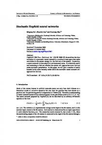
For these objectives, constraints, and forward and backward changes of variable, the change of variable conditions () are proven to hold in Appendix I. The advantage of the new system is that all polynomial degrees are low (3 or 4 rather than L). However, the overly numerous (s)-indexed variables remain. The objective and constraints of (5) and (6) may be diagrammed as shown below, in which the small open circles are variables, the ovals represent the models (which store constant database infor mation like u, ', H, and INA), and the squares are possible terms in a derivation. Each diagram below shows only a representative clique of related variables which interact in one constraint in a conjunction thereof or one summand of the objective function. Links connect variables which share an index. The objective function and the inequality constraint are shown in these two diagrams, with object types on the left and instances (grammatical “object” terms and their associated parameters, x) on the right of each diagram: !

l-1 !

A(s)

(s1 ...sl-1)

(!!) !

l-1 x(s)

l-1 !

A(s)

(s1 ...sl-1)

prefix

prefix 789

l x(s)

"

" Al(s)

2 !!!"

(s1 ...sl ) (s1 ...sl )

"

" Al(s) +C(s)l "

Figure 2: Aliveness variables in objective and constraint.

Symbolic Neural Networks Derived from Stochastic Grammar Domain Models

5

3.1.1 Specialization to Point-Matching We can make contact with previous experiments on nonhierarchical point-matching by specializing the aliveness variable formulation of the constrained optimization problem. If there is only one model accessible after L levels of derivation, say the L L" L “point” model, then A # s $ = 5 "% point Aˆ # s $ and we can substitute x # s $ = + # s $ P # s $ k x k into the l=L summand of the objective and simplify. By specializing H to include translational an rotational degrees of freedom at every node in the hierarchy, we arrive at the objective & 0' E # A% x $ = H 0 $ x % +

L–1

l "

+ + + A s "s 1

l

A

!s l " l l–1 l–1 1 --------- x s1 "sl – x s1 "sl – 1 – :s1 "sl – 1 ; y 2 22 l

l – 1! s 1 "s l – 1

l = 1 # s $ !"

+ +++

L – 1! A s1 "sl – 1

P # s$ k

k # s$ !

1 --------- x 2 22 L

L k

–

L–1 x s1 "sl – 1

–

L–1 :s1 "sl – 1

;y

!s l point 2

2

# sl "$ & l–1 ' + G $ :s1 "sl – 1 % 2 l% 2 l – 1 % – '

(7) # s l point $ & L–1 ' + G $ :s1 "sl – 1 % 2 L% 2 L – 1 % – '

and the constraints A% Aˆ % P% INA 0 ( 0% 1 ) A

0% !

l Aˆ # s $

A

l " s 1 "s l

= 5 !% root =

l "

+" A# s$

(8)

l – 1! 1 "s l – 1

* +! INA !s " A s l

+" INA!2" * 1 1

1

+ # s$ P # s$ k = < &$ k + --2- '% < &$ kmax – k + --2- '%

+k P # s$ k

)

L = Aˆ # s $

(Here < is the 0/1-valued Heaviside function, used to constrain k to be between 1 and its maximum.) This constrained optimization problem is a hierarchical generalization of a previous nonhierarchical (L=1 or 2) point-matching architecture implemented in [6]: 1 E # m% A% t% '% = $ = --------2- +ij m ij x i – t – Ay j 22

2

– ! +ij m ij – g # A $

with constraints m 0 ( 0% 1 ) ) +i m ij * 1 ) +j m ij * 1 . Here g is a regularizer on the affine transformation matrix A, and G is a similar regularizer for the affine transformation : between levels in the hierarchical object grammar, parameterized by the noise parameters 2. In particular if : is regularized to favor rotations, then we obtain a mobile-like hierarchical object model.

3.2 Mapping to Neural Networks An objective function such as equation (5), and its associated constraints (e.g. that each A is zero or one), can be mapped into an analog neural network by a variety of techniques [8][9] which require that we expand H into a polynomial, and allocate multi-way synapses for each monomial in the resultant polynomial expression for E. The constraints can be treated similarly. Monomials of degree two such as 3xy are mapped to a pair of conventional synapses from neuron x to neuron y and back. If the polynomials have a regular structure, the synapse count may be considerably reduced by introducing intermediate variables as in [12]. Convergence can often be greatly accelerated by introducing clocked dynamics as in [14]. The resulting networks will have a localist encoding because of the 0/1-valued A and P variables, which is an inefficient use of space since at least the permutation matrix P is sparse. It is possible that new mappings to localist [12] or distributed [22] representations will eventually allow the same model to run with much less circuitry. Effective use of deterministic annealing methods can also improve the quality of the local minima to which such algorithms converge, for both recognition and learning [6][5].

Symbolic Neural Networks Derived from Stochastic Grammar Domain Models

6

3.3 Eliminate Derivation Indices The (s) indices still introduce a rapidly, perhaps exponentially growing number of variables, corresponding to all the possible derivations in the grammar. Two further changes of variable can eliminate the excess variables. First, we introduce auxiliary variables P and x at all levels, not just l=L, and we eliminate the remaining choice variables C˜ . This step introduces trivial dependent “frame instances” in correspondence with the derivation objects. Second, we eliminate the derivation objects and their aliveness variables A in favor of the frame instances and relationships between them and between frames (models) and their instances. These changes are diagrammed in figure 3, using triangles to represent frame instances and showing all relevant variables in two neighboring cliques at levels (L-2, L-1) and (L-1, L). The dotted lines show the introduction of the new A

A

prefix

789

A

x

prefix

789

x

A

P alloc

prefix

789

x

A

x

alloc

P

alloc

x

P

A

x

x

M

A

alloc

P x

alloc

prefix

x

prefix

789

x

P

x

x

ina

789

789 A

P

x

alloc

prefix 789 A

alloc

M

ina

789

x

P

x

x

alloc

alloc

M

x

Figure 3: Change of variables to Frameville architecture. link types: the match or instantiation variables “M” between frame models and instances, and the Part-of variables “ina” between instances.

3.3.1 1st Change: Add Instances The change of variables is: A=A

Aˆ = Aˆ

) l

x

l j =

+

l P # s$ # s$ j

l x # s$

A=A

)

)

L

x = x

)

L

l

auxiliary variables: x j 0 >

3F :

L

P = P

)

l

) P# s $ j 0 ( 0% 1 ) # l & L $ % alloc j 0 ( 0% 1 )

+

l P # s$ # s$ j

= alloc

l j

+

)

l P j # s$ j

=

(9)

l Aˆ # s $

and inversely Aˆ = Aˆ l

x # s$ = 3B :

C˜ auxiliary variables:

l " # s$

P = P

)

l

+j P# s$ j

0 ( 0% 1 ) ) ˜ C

l " # s$

L

)

L

x = x

l

xj

˜ C

+"

l " # s$

l–1 l * Aˆ # s $ – Aˆ # s $

l – 1!

* +! INA !s " A # s $

Symbolic Neural Networks Derived from Stochastic Grammar Domain Models

L

l

(10)

l"

– A # s$

7

The new objective function is: & 0' E # A% x $ = H 0 $ x % +

L

l "

+ + + + INA!s " A s "s l

l = 1 s !" ij

1

l – 1!

l

l–1

A s1 "sl Ps1 "sl% j P s1 "sl – 1% i

l

H

# !s l " $ &

l

$ x j% x

l–1 i %

u

# !s l " $ '

% –'

# sl "$

(11)

The constraints for the (A, P, alloc, x) variables are: A% Aˆ % P% alloc% INA 0 ( 0% 1 ) A

0% !

l Aˆ # s $

A

l " s 1 "s l l

+ # s$ P# s$ j

= 5 !% root =

L

x k = xk

) l "

+" A# s$

L 1 1 alloc k = < &$ k + --- '% < &$ k max – k + --- '% 2 2

)

l l–1 Aˆ # s $ * Aˆ # s $

)

(12)

l – 1! 1 "s l – 1

* +! INA !s " As l

l

= alloc j

l = Aˆ s

l

+j P# s$ j

)

The validity of this change of variables is proven in Appendix II.

3.3.2 2nd Change: Eliminate Path Indices Now we eliminate all the exponentially growing derivation path indices (s) by eliminating A and P. The change of variables is: (13) l

x =x

l

l

l

l

inaisl j = l

x =x A 3B :

l " # s$

=

l

+s "s 1

P# s $ j

l–1

l–1

l

P s1 "sl – 1% i l

P s1 "sl% j l

alloc j = alloc j

)

l

l

+j M"j P# s$ j P l

l

l "

+ # s$ A# s$

M"j =

3F :

l

alloc j = alloc j

)

P s1 "sl% j =

0

# $i

l Aˆ # s $ =

)

+" A

l " # s$

0

= M rooti l–1

l

+i inais j P s "s l

1

l – 1%

i

This is quadratic in the link variables A, P, M, and ina.

3.4 Frameville with Slots The resulting objective function and clique diagrams are shown below:

Symbolic Neural Networks Derived from Stochastic Grammar Domain Models

8

& 0' E # A% x $ = H 0 $ x % +

L

l

l– 1

+ + + INA!2" inai2j M !i

l

M "j H

# !2" $ &

$ x j% x

l

l–1 i %

xi

i

u

# !2" $ '

% –'

# 2" $

(14)

l = 1 !2" ij

M! i !

789

inai 2 j

2 !!!"

xj

"

j

M"j

Figure 4: Frameville objective. This objective is of polynomial degree five or a little more depending on H. Further reduction down to degree three is possible as in [12]. The constraints for the (M, ina, alloc, x) variables are: M% ina% alloc% INA 0 ( 0% 1 ) 0

+i M !i = l

5 !% root

)

L

x k = xk

)

L 1 1 alloc k = < &$ k + --- '% < &$ k max – k + --- '% 2 2

l

+" M "j

= alloc j

l

(15)

l

+i2inai2j

= alloc j

l

l– 1

+j ina i2j * alloc i l

l

l– 1

+j inai2j M "j * +! INA!2" M !i

The four constraint cliques relating different kinds of variables are diagrammed as before, in Figure 5. Again, the validity of

(!!) "

M "j j

allocj (!!) !

alloci

(!!) i

M! i i

inai 2j

i

inai 2j

inai2 j 789 !!!" 2 (!!) j

" M" j

j

allocj

(!!) j

Figure 5: Frameville constraints l

this change of variables is proven in Appendix II. Note that the +j ina i2j inequalities reflect the possibility of object deletions in the original grammar, which has not been hidden in this particular problem formulation. An earlier version of Frameville [18], [16], which did not have the slot index 2 on INA or ina and which specialized INA by restricting it to be a tree, can be derived (for tree INA’s) from this version by a further change of variables which we omit. A version including slot indices was related to predicate calculus in [1]. Related symbolic optimization architectures include [11], [21],[25].

3.4.1 Learning in Frameville Important aspects of the model base such as the constant parameters u and ' which tune the consistency function H, or the INA matrix which specifies the equivalent detailed grammar, may be learned by starting off the recursive object-generation grammar with extra “metagrammar” or “compound grammar” rules which first choose u and/or INA from a prior probability Symbolic Neural Networks Derived from Stochastic Grammar Domain Models

9

distribution, and then generate a number of scenes (rather than just one as above) which can be used as input to a learning algorithm. The resulting constrained optimization problem for learning the model base parameters u could for example be: E learn # u% '% ( M% ina% x% alloc ) ;INA $ =

&

p

p

p

+ Erecog $ M % ina % x % alloc

p

' ;u% '% INA %

p

!2" 1 + ------------ + u 2 22 u !2"

2

2" 1 + -----------2- + ' 22 u 2"

2

+ '˜ + INA !2"

(16)

!2"

if the prior on u and ' is taken to be Gaussian and that on INA is taken to be independent on each two-valued matrix entry, subject to the INA constraint. This type of learning problem has been solved efficiently with neural networks for the simpler point-matching problems that arise in nonhierarchical generative grammar models [5].

4.0 Discussion In this version of the Frameville architecture, by comparison with earlier versions [18][17], we can see several advantages and limitations. The depth of a derivation is bounded by the arbitrary integer L. Any number of “distractor” or noise objects can be modelled as parts of a level-one “background” object. The model-side compositional hierarchy INA !" = +2 INA !2" is a general graph, rather than being limited to a tree or a DAG. The stochastic grammar can be extended to define modellearning as another constrained optimization problem, in which the bias of the learning algorithm is explicitly given by a prior probability distribution on model bases in the compound grammar rather than implicitly given by a neural net wiring diagram. And as before, the number of required variables grows as a low power of the size of the data, and the architecture can be diagrammed with a 3D embedding that suggests control flow strategies. On the other hand, the Frameville architecture presented here is missing several crucial link types (such as explicit ISA, EQU for equality of frame instances, SIB for siblings in the composition hierarchy, and so on); the data-side dynamic ina links are restricted to form a tree (a restriction removed by EQU for translating predicates in [1]; see also [15]); the remaining slot indices 2 are inconvenient for large collection objects; all variables remain indexed by their level numbers in the grammar derivation; and we have not exhibited a neural dynamics, or other global constrained optimization algorithm, which can solve the Frameville optimization problems in a scalable way as has been done for less difficult optimization problems.

4.1 Comparison with Other Integration Schemes Bayesian networks [19] are analogous to derivations of our grammar, in that they have conditionally independent probability distributions forming an underlying stochastic domain model, they can be learned, and they provide a high-level language for integrating multiple process models. They have the important expressive advantage that they are DAGs, rather than trees as our derivations are; so they are “multiple cause models” [24]. We have formulated context-sensitive deterministic L-system grammars whose derivations are DAGs, for use in biology [15], and a similar generalization may be possible here. But in a Bayesian net each node’s probability distribution tends to be much less powerful than our Boltzmann distributions, and there is no grammar inducing structure or regularity on the derivation tree. Also there is no analog of the “correspondence” or “variable-binding” problem introduced by relabelling the data according to the random permutation matrix P, which speeds up the computations but limits the expressive power of the Bayesian networks.A related trend in machine learning is the introduction A related trend in machine learning is the introduction and formalization of appropriate “structure” in a model class by model-generation procedures. A Minimum Description Length approach to neural net learning [7] and Hidden Markov Model-generating neural networks [2] are recent examples. Our grammar schemata may be viewed as procedures for generating models, with appropriate structure, in the following model classes: (1) larger parameterized L-system grammars; (2) simplified semantic networks; (3) Bayesian net-like grammar derivations; (4) constrained optimization problem formulations; and (5) relaxation-based neural networks. A stochastic grammar formalism may be especially expressive in this role. There are a number of neural network architectures which do variable-binding [4][10][21][25], some of which are relaxationbased networks which pose constrained optimization problems. Some of our work on transformations from optimization problems to neural networks could be applied to those systems as well. The stochastic grammar approach avoids the common problem of creating slightly extended implementations of symbolic processing in neural networks, rather than true integration of the advantages of each, by starting with an underlying statistical domain model. From this model emerge domain-specific “distance” or “similarity” measures for pattern recognition and learning on structured objects. If a statistical domain model is Symbolic Neural Networks Derived from Stochastic Grammar Domain Models

10

simple enough one may derive algorithms close to ordinary neural networks, including learning [3]. Otherwise, we find mixed logical and numerical processing in a more elaborate architecture. The grammar and therefore the network architecture can be tuned to specific domains (such as high-level vision) by including domain-specific grammar rules (such as the geometric invariances of objects [16]) which get hard-wired into the resulting neural networks. For highly expressive architectures one generally cannot claim more or less complete expressiveness, only more or less appropriate expressiveness. Further work on the stochastic grammar approach will determine whether such claims should be made about it. Acknowledgment. Gary Cottrell provided many useful comments in the preparation of this paper.

References 1. P. Anandan, S. Letovsky, and E. Mjolsness. Connectionist variable-binding by optimization. Proceedings of the Cognitive Science conference, August 1989. 2. P. Baldi and Y. Chauvin. Hybrid modeling, HMM/NN architectures, and protein applications. Neural Computation, in press. 3. B. Cheng and D. M. Titterington. Neural networks: A review from a statistical perspective. Statistical Sciences, v. 9 n. 1, pp. 2-54, 1994. 4.

M. Derthick. Mundane Reasoning by Parallel Constraint Satisfaction. Morgan-Kaufmann 1990.

5. S. Gold, A. Rangarajan, and E. Mjolsness. Learning with preknowledge: Clustering with point and graph matching distance measures. Neural Computation, in press. Preliminary version in: Neural Information Processing Systems 7, MIT Press 1995. 6. S. Gold, C. P. Lu, A. Rangarajan, S. Pappu, and E. Mjolsness. New algorithms for 2D and 3D point matching: Pose estimation and correspondence. In: Neural Information Processing Systems 7, MIT Press 1995. 7. G. Hinton and R. Zemel. Autoencoders, minimum description length and Helmholtz free energy. Advances in Neural Information Processing Systems 6, eds. J. Cowan, G. Tesauro, and J. Alspector, Morgan Kauffman 1994. 8. J. J. Hopfield. Neurons with graded response have collective computational properties like those of two-state neurons. Proceedings of the National Academy of Sciences USA, v. 81, p. 3088-3092, 1984. 9. J. J. Kosowsky and A. L. Yuille, The invisible hand algorithm: Solving the assignment problem with statistical physics. Neural Networks 7(3):477-490, 1994. 10. T. Lange,. and M. G. Dyer. Dynamic, non-local role-bindings and inferencing in a localist network for natural language understanding. In David S. Touretzky (ed.), Advances in Neural Information Processing Systems 1, pp. 545-552. MorganKaufmann, 1988. 11. C. von der Malsburg and E. Bienenstock. Statistical coding and short-term synaptic plasticity: A scheme for knowledge representation in the brain. In Disordered Systems and Biological Organization, 247-252, Springer-Verlag 1986. 12. E. Mjolsness and C. Garrett. Algebraic transformations of objective functions. Neural Networks, 3:651-669, 1990. 13. E. Mjolsness, C. Garrett, and W. Miranker. Multiscale optimization in neural networks, IEEE Transactions on Neural Networks, vol 2 no 2, March 1991. 14. E. Mjolsness and W. Miranker. Greedy Lagrangians for Neural Networks: Three Levels of Optimization in Relaxation Dynamics. Technical Report YALEU/DCS/TR-945, Yale Computer Science Department, January 1993. 15. E. Mjolsness, D. H. Sharp, and J. Reinitz. A connectionist model of development. Journal of Theoretical Biology, 152(4):429-454, 1991. 16. E. Mjolsness. Bayesian inference on visual grammars by neural nets that optimize. Technical Report YALEU/DCS/TR854, Yale Computer Science Department, May 1991. Available on neuroprose and at URL http://www-cse.ucsd.edu/users/ emj .

Symbolic Neural Networks Derived from Stochastic Grammar Domain Models

11

17. E. Mjolsness. Connectionist grammars for high-level vision, in Artificial Intelligence and Neural Networks: Steps Toward Principled Integration, eds. Vasant Honavar and Leonard Uhr, Academic Press, 1994. 18. E. Mjolsness, G. Gindi, and P. Anandan. Optimization in model matching and perceptual organization. Neural Computation 1(2), 1989. 19. J. Pearl. Probabilistic Reasoning in Intelligent Systems: Networks of Plausible Inference. Morgan-Kaufmann, 1988. 20. C. Peterson and B. Soderberg. A new method for mapping optimization problems onto neural networks. International Journal of Neural Systems, 1(3), 1989. 21. G. Pinkas. Energy minimization and the satisfiability of propositional calculus. Neural Computation 3(2), 1991. 22. T. Plate. Distributed representations and nested compositional structures. PhD thesis, Department of Computer Science, University of Toronto, 1994. 23. P. Prusinkiewicz. The Algorithmic Beauty of Plants. Springer-Verlag New york, 1990. 24. E. Saund. A multiple cause mixture model for unsupervised learning. Neural Computation, v. 7, n. 1, 1995. 25. A. Stolcke. Unification as Constraint Satisfaction in Structured Connectionist Networks. 26. D. E. Van den Bout and T. K. Miller, III. Graph partitioning using annealed networks. IEEE Transactions on Neural Networks, 1(2):192-203, 1990.

Appendix I We prove the validity, according to the criterion of equation (3) with temperature T=0, of the change of variable (4) from rule choice variables C to term aliveness variables A.. First we show that the constraints on C (equation (2)), and the forward change of variables 3 F (equation (4)), imply the constraints on A (equation (6)), i.e. C C ) 3 F 1 C A . Clearly 3 F preserves the 0/1-valuedness of all the variables. The condition on A CC ) 3F

we can calculate

l" A " # s$

+

l l" l A * ( # s $ = Aˆ # s $ , and " # s$ l k l l l ( * ( # s$ = ( # s$ ( # s$ * k = 1 # s$

+ ,

we l ( # s$

=

l ( # s$

have

l" C " # s$

+

proven

k l–1 ( k = 1 # s$

,

6

l l ( # s$ ( # s$

, so

l ( # s$

two =

=

l ( # s$

=

l Aˆ # s $

inequalities k l ( k = 1 # s$

,

0% !

is unchanged in C A from C C . From l

l"

l

k

; but ( # s $ +" C # s $ * ( # s $ ,kl –=11 ( # s $

implying

l" A " # s$

+

=

l Aˆ # s $

.

Note

so also

.

The constraints on x and P are direct translations under 3 F , from C C to C A . So we only have to derive the two inequalities on l" ˜ and A, in C . We can calculate Aˆ l + C # s$ +" C˜ # s$ = A l"

k

l–1

l–1

+" C # s$ * ,k = 1 ( # s$ , which equals ( # s$

for l 6 2

&

l"

l"

'

l"

l

l

l"

+" $ A # s$ + C˜ # s$ % = +" C # s$ ( # s$ + 1 – ( # s$ = +" C # s$ . But 0 l–1 (otherwise l=1 and , = 1 = Aˆ ), which is Aˆ # s $ by 3 F . This establ"

l"

l"

l

l

lishes the first inequality. For the second inequality, calculate A # s $ + C˜ # s $ = C # s $ ( # s $ + 1 – ( # s $

l"

= C # s $ , which

l – 1!

is * +! INA !s " C # s $ , as required. l

So C C ) 3 F 1 C A . Next we must show C C ) 3 F 1 3 B . But 3 B follows trivially from 3 F alone. Now we must show that the constraints on A (equation (6)), and the backward change of variables 3 B (equation (4)), imply the constraints on C (equation (2)), i.e. C A ) 3 B 1 C C . Clearly 3 B preserves the 0/1-valuedness of the ( and P variables. l"

l"

l

l"

l–1

However, the C variables could also take on the value 1+1=2, except that C # s $ * +" C # s $ = Aˆ # s $ + +" C˜ # s $ * Aˆ # s $ * 1 . The constraints on

l"

+" C # s$

in C C may be verified as follows. From 3 B ,

other hand we have already calculated that (as required for

l"

l–1

k

+" C # s$ * ,k = 1 ( # s$ )

l"

+" C # s$

l"

+" C # s$

l ˜ l" 6 Aˆ l = ( l . On the = Aˆ # s $ + +" C # s$ # s$ # s$

l ˜ l" * Aˆ l – 1 , which is = Aˆ # s $ + +" C # s$ # s$

* 1 for l=1, and

l–1

= ( # s $ for l=2

and also for all larger values of l. But by induction on l, for l 6 2 we have

Symbolic Neural Networks Derived from Stochastic Grammar Domain Models

12

l–1

l–1

l–1

l–1

( # s$ = ( # s$ ( # s$ * ( # s$

that

k l ( k = 1 # s$

,

=

l ( # s$

k

l–2

,k = 1 ( # s$

k

l–1

l"

k

l–1

,k = 1 ( # s$ , which establishes +" C # s$ * ,k = 1 ( # s$

=

for all l. As a corollary, we see

, and therefore the constraints on x and P in C C are a direct translation of those in C A .

l" l" l – 1! The last constraint in C C is C # s $ * +! INA !s " C # s $ , which we prove using 3 B and nonnegativity of INA !s " and C˜ # s $ : l

l – 1!

+! INA!s " C # s$ l

l"

– C # s$ =

l

l – 1! ' l" l" & l – 1! l" l – 1! l" +! INA!s " $ A # s$ + C˜ # s$ % – A # s$ – C˜ # s$ 6 +! INA!s " As – A # s$ – C˜ # s$ , which is 6 0 by CA . l

l

Next we show that C A ) 3 B 1 3 F : The conditions on A l" l C # s$ ( # s$

0

l

by 3 B . l" l l l" ˆ l l" ˜ = A # s $ A # s $ + C # s $ Aˆ # s $ . Evaluate the summands: Aˆ # s $ = A implies (for 0/1 variables) " # s$ l" l l l" l l – 1 l l l l & ' ˜ Aˆ ˜ ˆ C C * Aˆ s $ Aˆ # s $ – Aˆ # s $ % = Aˆ # s $ – Aˆ # s $ = 0 , Aˆ # s $ and since # s$ # s$ * A # s$ " # s$ l" l" l l" & l ' Substituting, we find A # s $ = C # s $ ( # s $ as desired. Likewise C # s $ $ 1 – ( # s $ % = ˜ l" – C ˜ l" Aˆ l + A l" & 1 – Aˆ l ' = C˜ l" – 0 + 0 , as desired. = C # s$ # s$ # s$ # s$ % # s$ # s$ $

& l" ˜ l" ' Aˆ l = $ A # s$ + C # s$ % # s$

l l" l" A # s $ Aˆ # s $ = A # s $ , that l ˜ l" * Aˆ l – 1 . * Aˆ # s $ + " C # s$ # s$ l" ' & l ' & l" ˜ = $ A # s $ + C # s $ % $ 1 – Aˆ # s $ %

+

l

follow directly from C A . Aˆ # s $ = ( # s $

+

+

Finally we must translate the objective, assuming C C ) 3 F ) C A ) 3 B . Using the calculations in the proof above, we can work out l" l – 1! & C s "s . "s 1 l 1 l

Cs

l

'

k

, ( s "s /% $ 1

k=1

l

l" l – 1! l C ( # s$ 1 "s l s 1 "s l

= Cs

& l" ˜ l" ' & A l – 1! + C ˜ l – 1! ' Aˆ l = $ A # s$ + C # s$ % $ # s$ # s$ % # s$ l" l – 1! ˆ l As

l l" l – 1! l l – 1 l – 1! & l" ˜ ˜ l" ' + Aˆ s C˜ s A s + Aˆ # s $ Aˆ # s $ C # s$ $ A # s$ + C # s$ %

l" l – 1! ˆ l As

+ 0A s

= As As = As As

l – 1!

l l" ' & l" + Aˆ # s $ 0 $ A # s $ + C˜ # s $ %

l" l – 1!

= As As

Substituting this result into equation (1), after using &$ ,kl = 1 ( equation (5) as desired.

k

' l s 1 "s l % ( # s $

=

k

l

,k = 1 ( s "s 1

l

to simplify the ' term, yields

Appendix II We now prove the validity, according to the criterion of equation (3) with temperature T=0, of the change of variable (9),(10) which adds dependent permutation variables P at each level in the hierarchy, and also the change of variable (13) which completes the derivation of Frameville. First we show the validity of the change of variables (9), (10), from C A (equation (6)) to C A% P (equation (12)). For the most part, this change of variables just consists of adding and removing auxiliary variables, i.e. variables in X\x orY\y, in the notation of section 3.0. These changes would affect the entropy terms (omitted in this paper) in the free energy expressions at nonzero temperature. In C A , which is mapped to C A% P via 3 F , the auxiliary variables are the C˜ ‘s. In C A% P , which is mapped l l l back to C A via 3 B , the auxiliary variables are those x j and P j for which l & L , together with alloc j . Most of the constraints on nonauxiliary variables are explicitly preserved between C A and C A% P . There are only a few details to check. l

l–1

l"

l"

l"

In the forward direction, it is not explicit in C A that Aˆ # s $ * Aˆ # s $ . It is, however, implicit: A # s $ * A # s $ + C˜ # s $ * l – 1!

+! INA!s " A # s$ l

l" & l – 1! ' ˆl–1 ˆl * +! $ A s % = A # s $ ; but since A s 0 ( 0% 1 ) and A # s $ =

l"

+" A # s$ 0 ( 0% 1) , we have

l l" Aˆ # s $ = max " A s

l–1 l–1 L * max " Aˆ # s $ = Aˆ # s $ . The expansion for alloc k in C A% P in terms of Heaviside < functions just says alloc=1 if k is in {1, 2,

... k max }, otherwise alloc=0. This just names the domain of allowed k’s in C A ‘s constraints on x and P. We must also check that the required auxiliary variables exist, i.e. that their constraints are consistent. The auxiliary x’s are uniquely determined by the regular x’s and the auxiliary P’s, which are in turn constrained by permutation-like constraints which can be satisfied in many ways. The C˜ variables are constrained by 3 B to be less than or equal to quantities which are guaranteed by C A% P to be nonnegative, so that at least the configuration C˜ = 0 is consistent. Symbolic Neural Networks Derived from Stochastic Grammar Domain Models

13

l"

l" l – 1!

l – 1!

Finally we must translate the objective. We first show A # s $ A # s $ l"

l"'

l"

l – 1! l – 1!'

know that A # s $ A # s $ = 5 ""' A # s $ , and likewise A # s $ A # s $ l"

l – 1!

INA !s " A # s $ A # s $ l

l"

= INA !s " A A # s $ l – 1!

= 5 !!' A # s $

l – 1!

s

l

l"

. Since

l"

+" A # s$

l = Aˆ # s $ 0 ( 0% 1 ) , we

. Therefore

l"

l – 1!

= A # s$ A # s$ A # s$

* A # s$ A # s$

l" l – 1!' l – 1! * A # s $ &$ +!' INA !'s " A # s $ '% A # s $ l

l" A # s$

=

l – 1!' l – 1! A # s$

+!' INA!'s " A # s$ l

l"

l – 1!

= A # s $ +!' INA !'s " 5 !!' A # s $ l

l" l – 1!

= INA !s " A A # s $ s

l

l

as desired. Using this fact, and substituting x # s $ = l" l – 1!

As A # s$

H

# !s l " $ & l l – 1 # !s l " $ ' $ x # s $ % x # s $ ;u %

–'

# sl "$

l

l

+j P # s$ j xj , we can calculate l" l – 1!

= INA !s " A A # s $ s

l

H

# !s l " $ &

l

l" l – 1! l l–1 P # s$ j P # s$ i

+ij INA!s " As A # s$

=

l

in which the last step follows from the winner-take-all constraints

l

l–1 l–1

$ + j P # s $ j x j% + i P # s $ i x i

l

+j P # s$ j

H

;u

# !s l " $ '

% –'

# !s l " $ & l l – 1 # !s l " $ ' $ x j% x i ;u %

l = Aˆ # s $ and

l–1

+i P # s$ i

–'

# sl "$

# sl "$

l–1 = Aˆ # s $ for 0/1 variables, in

l l–1 which Aˆ # s $ = 1 and Aˆ # s $ = 1 for any nonzero instance of the above expressions. Substituting this result into the objective of

equation (5) yields the objective of equation (11), as desired. Thus we have proven the validity of the first change of variables.

Now we show the validity of the change of variables (13) from C A% P (equation (12)) to C M (equation (15)). The constraints on x, alloc and INA are unchanged. First we show C A% P ) 3 F 1 C M . To show that M and ina are 0/1-valued variables, we bound l

ina isl j = l M i !j

+

their

expressions l–1

+s "s P s "s 0! 0 = +i% # s $ A # $ P # $ i 1

l–1

1

l – 1%

in

l i P s 1 "s l% j

*

+s "s

0 P i # $i

= 5 !root +

l

3F : 1

P l–1

l–1

M "j = s 1 "s l – 1% i

+ # s$ A l–1

= alloc i

0

l"

l # s$ P # s$ j

* + # s$ P

l

# s$ j

l

= alloc j * 1 ,

and

* 1 . The level-0 boundary condition on M is:

0

= 5 !root Aˆ = 5 !roo, since Aˆ = 1 .

For the allocation constraint on M, we calculate that

l

&

l"

'

l

l

l

+ # s$ P # s$ j = allocj , where we l l l l l–1 l have used P # s $ j * +j P # s $ j = Aˆ # s $ . Likewise for the allocation constraints on ina, +i2 ina i2j = + # s $ &$ +i P # s $ i '% P # s $ j l–1 l l–1 l l l l l l l l = + # s $ Aˆ # s $ P # s $ j = + # s $ P # s $ j = alloc j , where we have used Aˆ # s $ P # s $ j * P # s $ j = P # s $ j P # s $ j * P # s $ j +j P # s $ j = l l–1 l l–1 l–1 l l l l l–1 & ' l–1 = P # s $ j Aˆ # s $ * P # s $ j Aˆ # s $ . On the other hand, +j ina i2j = + # s $ $ +j P # s2 $ j % P # s $ i = + # s $ Aˆ # s2 $ P # s $ i * + # s $ Aˆ # s $ P # s $ j l–1 l–1 l–1 l–1 l–1 l–1 l–1 l–1 l–1 l–1 l–1 = + # s $ P # s $ j = alloc i , where we have used Aˆ # s $ P # s $ j * P # s $ j = P # s $ j P # s $ j * P # s $ j +j P # s $ j = P # s $ j Aˆ # s $ . +" M"j

Symbolic Neural Networks Derived from Stochastic Grammar Domain Models

=

+ # s$ $ +" A # s$ % P # s$ j

=

14

The rectangle constraint on ina, INA and M is derived in another calculation: l

l

+j inai2j M"j

l"

l

l–1

l

l

l

=

+ # s$ + # s'$ +j A # s'$ P # s'$ j P # s$ i P # s2$ j

=

+ # s$ + # s'$ A # s'$ P # s$ i +j P # s'$ j P # s2$ j

=

+ # s$ + # s'$ A # s'$ P # s$ i 5 # s'$ # s2$ Aˆ # s'$

=

+ # s'$ A # s'2$ P # s'$ i

l"

l"

l–1

l"

l–1

l

l–1

l – 1! l – 1

* +! INA !2" + # s' $ A # s' $ P # s' $ i =

l–1

+! INA!2" M!i

l"

l

So we have shown C A% P ) 3 F 1 C M . Next we show C A% P ) 3 F 1 3 B . For this we must show A # s $ = l P # s2 $ j

l l–1 ina i2j P # s $ i . i l l–1 ina i2j P # s $ i i

+ Likewise, + =

Substituting from 3 F , =

+

l P # s' $ # s'2 $ j

l l M P j "j # s $ j

+

l–1 l–1 P P i # s' $ i # s $ i

+

=

+

l l = P P j # s' $ j # s $ j l–1 l l P 5 Aˆ = P # s2 $ j # s' $ # s'2 $ j # s' $ # s $ # s $

+

l" A # s' $ # s' $

+

+

=

l l" A 5 Aˆ # s' $ # s' $ # s' $ # s $ # s $

0! 0 A# $P# $i

=

=

0 5 !root P # $ i

=

and

l" A # s$

.

, as desired. In addition, the rela-

0 tion between A and Aˆ variables is directly present in C A% P and the expression for P # 0 M !i

l

+j M"j P # s$ j

follows from 3 F :

$i

. So C A% P ) 3 F 1 3 B .

Now we need to establish the backwards direction, C M ) 3 B 1 C A% P ) 3 F , starting with C M ) 3 B 1 C A% P . That alloc is a 0/1valued variable is direct. For the A and Aˆ variables, their expressions in 3 B are non-negative integers and we can bound them by one at the same time that we establish the summation and 0/1 constraints on P, using induction on l. For the base case, 0! $

0

* Aˆ #

0

0

0

0

0

2

0

+!i M!i Mrooti = (since +! M!i * 1 ) +! 5!root +i Mrooti = +! # 5!root$ =1, as desired. Also, 0 0 0 0 0 0 0 0 * +! M !i = alloc i ; on the other hand + # $ P # $ i = P # $ i = Mrooti +! M!i = Mrooti + +! ? root M!i * 0 0 ' 0 0 0 & M rooti + +! ? root $ +i M !i % = M rooti , so + # $ P # $ i = alloc i 0 ( 0% 1 ) . From this fact we can also deduce 0 l 0 0 l 0 0 l" Aˆ # $ = +!j M !i P # $ j = +j allocj P # $ j = +j P # $ j . The induction step is: for A, A # s2$ * Aˆ # s2$ l–1 l ' l l l l l l–1 l–1 l–1 & = +j $ +" M "j % P # s2 $ j = +j alloc j P # s2 $ j * +j P # s2 $ j = +ij ina i2j P # s $ i * +i alloc i P # s $ i which is, by induction, = Aˆ # s $ . l l l–1 l l–1 l l = +i2 ina i2j alloc i = +i2 ina i2j = alloc j . From this equality, we can also For P, + # s2 $ P # s2 $ j = +i2 ina i2j &$ + # s $ P # s $ i '% l l l l l l l l l = +j P # s $ j . Finally P # s $ j * +j P # s $ j = Aˆ # s $ * 1 .This proves all the relededuce Aˆ # s $ = +"j M "j P # s $ j = +j alloc j P # s $ j A#

$

=

+!i M!i P #

$i

=

vant 0/1-valuedness constraints, and the summation constraints on P. 0! $

The value of = # 5 !root $ =

l

2

+j P # s2$ j

A#

may be computed as with

0 Aˆ #

$

:

0! $

A#

=

l l–1 = 5 !root . Aˆ # s2 $ * Aˆ # s $ That follows from what l–1 l ' l–1 l–1 l–1 l–1 & = +i $ +j ina i2j % P # s $ i * +i alloc i P # s $ i = +i P # s $ i = Aˆ # s $ .

0

0

+i M!i P # has

l"

l–1 l–1 P # s$ i

+!i INA!2" M!i

=

l–1 l–1 P # s$ i

+! INA!2" +i M!i

=

l – 1!

+! INA!2" A # s$

0

l

been

l

+j M"j P # s2$ j

l

l

l–1

l

l–1

l l M "j alloc j

=

l M "j

l

ina i2j . The expression for M is: =

l M "j

+

l P # s2 $ # s $ j

0

=

= 5 !root +i M rooti l Aˆ # s2 $

proven:

l

l

l–1

+i +j inai2j M"j P # s$ i

. So we have proven C M ) 3 B 1 C A% P . l–1

Next we prove C M ) 3 B 1 3 F . The expression for ina can be verified simply: + # s $ P # s2 $ j P # s $ i =

+i' inai'2j alloci 5ii' = inai2j alloci = l l l l + # s2$ j' M"j' 5j'j P # s$ j = + # s2$ M"j P # s2$ j

0

+i M!i Mrooti

=

already

The last component of C A% P is the INA inequality. It is computed as follows: A # s2 $ = *

$i

l"

l

+ # s2$ A # s2$ P # s2$ j

=

l

l–1

l–1

+i' # s$ inai'2j P # s$ i' P # s$ i = l l l + # s2$ j' M"j' P # s2$ j' P # s2$ j =

= (by C A% P which has already been proven from C M ) 3 B )

. The other components of 3 F are trivial. So we have proven C M ) 3 B 1 3 F .

Symbolic Neural Networks Derived from Stochastic Grammar Domain Models

15

l–1

Now we need only translate the objective function. To this end, we use l l P # s'2 $ j P # s2 $ j

=

l 5 # s' $ # s $ P # s2 $ j

l"

l–1

P # s' $ i P # s $ i = 5 # s' $

l–1 # s$ P # s$ i

and

to calculate

l – 1! l l – 1 # !2" $ P # s2 $ j P # s $ i H

+!" +ij + # s2$ INA!2" A # s2$ A # s$

# x i% x j $ = =

l"

l – 1! l l – 1 # !2" $ P # s2 $ j P # s $ i H

+!" +ij + # s2$ INA!2" A # s2$ A # s$ l"

# x i% x j $

l – 1!

+!2" +ij + # ss's''$ INA!2" A # s'2$ A # s''$ l

l–1

l

l–1

* P # s'2 $ j P # s'' $ i P # s2 $ j P # s $ i H l

l–1

l–1

# !2" $

=

+!2" +ij INA!2" inai2j M"j M!i

l

l

l–1

# x i% x j $ + # s $ P # s2 $ j P # s $ i

+!2" +ij INA!2" M"j M!i

H

l

# !2" $

=

H

# x i% x j $

(where we have used the fact that H depends on 2 but not (s)) which shows the desired equivalence of objective functions.

Symbolic Neural Networks Derived from Stochastic Grammar Domain Models

16