texture, and both are based on the principle that the vanishing point of a set of parallel ... P. We use homogeneous coordinates for image points p, so they are also 3- vectors. ..... For if we have corresponding points as input there is clearly no.
Structure from Motion of Parallel Lines Patrick Baker1 and Yiannis Aloimonos1 Center for Automation Research AV Williams Bldg University of Maryland College Park, Maryland 20742 {pbaker,yiannis}@cfar.umd.edu
Abstract. We investigate the camera geometry of lines parallel in the world. In particular, we formalize the known rotational constraints and add new linear constraints on camera position. The constraints on camera position do not require the cameras to be viewing the same lines, thus providing applications for occluded scenes and calibration of cameras for which fields of view do not intersect. The constraints can also be viewed as constraints of camera geometry with planar patch coordinate systems, and provide a way to investigate texture in a deeper way than has been done to date.
1
Introduction
The geometry of parallel lines has been used extensively in computer vision, but to our knowledge only by way of the plane at infinity using the computation of vanishing points. The two main applications are calibration and shape from texture, and both are based on the principle that the vanishing point of a set of parallel lines is not affected by translation, as it lies on the plane at infinity. While these are important applications, there are geometric relations on sets of parallel lines embedded in a planar patch, which take into account distances between the lines rather than just their vanishing point. Vanishing points have been used by many in computer vision, mostly for the determination of rotation and calibration for which they are particularly well suited, since they are unaffected by translation. There are numerous examples [1, 3]. These methods have not looked further into the lines of which the vanishing points are composed, but it is helpful to look at the individual lines. Lines have been used extensively in computer vision [5, 7, 4], but in general have not been as prominent as points, probably because they are difficult to work with. However, the use of of Pl¨ ucker coordinates [6, 2, 8] can make many reconstruction and constraint derivations easier. In this paper we introduce an extension of the Pl¨ ucker coordinates for lines in order to investigate lines embedded in a plane.
2
Notation and Reconstruction
Our use of parallelism restricts our world points to be represented by 3-vectors P. We use homogeneous coordinates for image points p, so they are also 3vectors. Image lines are also represented by homogeneous 3-vectors ℓ. If a point p is on a line ℓ, then their coordinates are perpendicular pT ℓ = 0. We use the general linear B = KR to encapsulate a rotation followed by a calibration. For a matrix B, we use B −T to denote the inverse transpose of that matrix. Points ˆ and ˆℓ. Note and lines that we actually measure in an image we denote by p −T −T ˆ = B(ℓ1 × ℓ2 ), then p ˆ = (B ℓ1 )× (B ℓ2 ). For clarity, in equations that if p we often use p and ℓ, which denote the calibrated and derotated coordinates for those points and lines.
2.1
Lines
We use the Pl¨ ucker coordinate system for world lines, which is particularly well suited for rigid motions of lines. Definition 1. A world line L is the set of all the points P ∈ R3 such that P = (1 − λ)Q1 + λQ2 for two� points Qi , and some scalar λ. The Pl¨ ucker � coordinates of this line are L = LLmd , where: Ld = Q2 − Q1 Lm = Ld ×P
direction of L moment of L
(1) (2)
If we have a line L and a camera (B, T), then the image line associated with L is ˆℓ = B −T (Lm − T×Ld ) (3) where ˆℓ is perpendicular to the plane containing the line in the image. If B is the rotation/calibration matrix for a point P, then B −T is the rotation/calibration matrix for a line L. Lines are easier to reconstruct than points because the reconstruction always exists. It is easily proved that: Proposition 1. If we have a line L in space which projects to two image lines ˆℓ1 and ˆℓ2 in distinct cameras (B1 , T1 ), and (B2 , T2 ), then we can calculate the coordinates for L if |ℓ1 ×ℓ2 | = 6 0, if ℓi = BiT ˆℓi : L=
�
ℓ1 ×ℓ2 ℓ1 TT2 ℓ2 − ℓ2 TT1 ℓ1
�
(4)
It is possible that the cross product above will be zero. In this case the line exists in the plane at infinity.
2.2
Singly Textured Planes
We introduce a new object to computer vision to encapsulate a set of parallel lines embedded in a plane. We motivate our definition as follows. Consider one line from the set of equally spaced lines in the� plane, � call it L0 . We may represent this line using Pl¨ ucker coordinates as L0 = LLmd . We take Q0 to be a point on L0 , and the point Qx = Q0 + xd to be on the line at distance x in the texture for some direction d. We can easily show that: Ld ×Q0 = Lm,0
(5)
so that to get Lm,n Lm,n = Ld ×Qx = Ld ×Q0 + xLd ×d = Lm + xLλ
(6) (7) (8)
where Lλ = Ld ×d. Note that since both Ld and d are vectors which lie inside the plane, we must have that Lλ is normal to the textured plane. This leads us to the following definition, as shown in figure 1 Definition 2. A singly textured plane H is a set of lines, equally spaced, embedded in a world plane. We give the textured plane coordinates Ld (9) H = Lm Lλ with LTd Lm = 0 and LTd Lλ = 0. The coordinates of each line in the plane, indexed by n are: � � Ld Ln = (10) Lm + nLλ Our constraints are all based on intersection conditions between two textured planes. Fact 1 If we have two textured planes H1 and H2 , then they lie on the same world plane if and only if: LTd,1 Lm,2 + LTd,2 Lm,1 = 0
(11)
and LTd,1 Lλ,2 = 0
LTd,2 Lλ,1 = 0
(12)
We now turn to the reconstruction of a textured plane from image lines in four cameras. This reconstruction is non-intuitive in a sense because we do not require that the cameras be looking at the same lines. Each of the four cameras can look at a different line. We only require that we know which line has been imaged, that is, its index n. Given these four lines we can reconstruct a textured plane, as in figure 2, with the following multilinear equation.
Fig. 1. The Parameters of a Textured Plane
Fig. 2. Reconstructing a Textured Plane
Fact 2 If we have a textured plane H which is imaged by four cameras into image lines ˆℓi , and we know that our cameras have parameters (Bi , Ti ), and further, we know that the image lines have indices ni , then we may reconstruct the textured plane as: Ld ni1 ni2 |ℓi3 ×ℓi4 |(ℓi1 ×ℓi2 ) X 2ni1 ni2 |ℓi1 ×ℓi2 |ℓi3 TTi ℓi4 (13) H = Lm = 4 2ni1 |ℓi2 ×ℓi3 |ℓi1 TTi4 ℓi4 Lλ [i1 i2 i3 i4 ]∈perm+ (1 2 3 4) Note that |·| is the signed magnitude, and since the coordinates are homogeneous, it does not matter which sign is chosen. The same result could be obtained by defining |ℓi ×ℓj | = |ℓj v ℓi | (14) where v is any arbitrary vector not in the plane of ℓi ×ℓj . The proof of this is in the supplement.
3
Rotational Constraints
If we have three image lines ˆℓi , each of which are images of one of a set of parallel world lines, then using two of the cameras we may reconstruct the direction Ld of the world lines. From the construction of the Pl¨ ucker lines, we know that any line with direction Ld must have moment vector perpendicular to Ld . Putting these two facts together, we obtain Proposition 2. If we have one, two, or three parallel world lines, and three cameras with rotation/calibration matrices Bi , then if these three cameras view images of one of our world lines as ˆℓi , with the lines not necessarily the same in all cameras, then we obtain the prismatic line constraint. ˆℓT B2 (B T ˆℓ1 ×B Tˆℓ3 ) = 0 2 1 3
(15)
If we identify cameras 2 and 1 by setting B2 = B1 , which corresponds to the case where both ℓ1 and ℓ2 are taken from the same camera. If these are different parallel lines, then we obtain the vanishing point constraint, noted by many, for example [9] Proposition 3. We have two or three parallel world lines, and two cameras with rotation/calibration matrices Bi . If camera 1 views image lines ˆℓ1 and ˆℓ3 and camera 2 views image line ˆℓ2 we obtain the vanishing point constraint. ˆℓT B2 B −1 (ˆℓ1 × ˆℓ3 ) = 0 2 1 T
ˆℓ B2 B −1 p 2 1 ˆ =0
(16) (17)
ˆ = ˆℓ1 × ˆℓ3 is called a vanishing point, and it is the point through The quantity p which all images of world lines of direction Ld will pass. The constraint says that if we have a vanishing point in one image and a line in another image which we know is parallel to the lines in the first camera, then we have a constraint on the Bi . If we further identify cameras 2 and 1, then given an image of a set of parallel lines in one camera, we know that we must still have a zero triple product. Proposition 4. We have three parallel world lines, and a camera with rotation/calibration nonlinear function B : R3 → R3 . Given images of these three world lines ˆℓi , i ∈ [1, . . . , 3]. We obtain the the vanishing point existence constraint. (18) |B T ˆℓ1 B T ˆℓ2 B T ˆℓ3 | = 0 This last constraint means nothing if B is a linear function, since the constraint would be trivally satisfied. However, in the case where there is some nonlinear distortion in the projection equation, there will be a constraint on B, so we may say that the prismatic line constraint operates on 1, 2, or 3 cameras. We next go over the standard multilinear constraints to show how the prismatic line constraint relates to them.
4
Translational Constraints
It is as simple to form the texture constraints as it was to form the previous constraint. There is a line texture constraint a point texture constraint, and a mixed constraint. Keep in mind that all these constraints can be applied to fewer cameras by identifying the camera positions associated with various subsets of lines. The first is the five camera constraint, which we call the harmonic trifocal, as shown in figure 3
Fig. 3. The Harmonic Trifocal Constraint operates on five image lines
Fact 3 If we have five cameras (Bi , Ti ), and measure five lines ˆℓi , which have indices ni from a textured plane H. We may form the ℓi using the ˆℓi and the Bi and have the following constraint: X (19) ni1 ni2 (ℓi1 ×ℓi2 )T (ℓi3 ×ℓi4 )TTi5 ℓi5 0= + [i1 ..i5 ]∈P [1..5] Where perm+ denote the even permutations. Proof. Using fact 2, we may reconstruct the textured plane to obtain the parameters of the textured plane H using the lines one through four. Using this reconstruction, we can find the fifth image line as: ℓ5 = Lm + n5 Lλ − T5 ×Ld
(20)
If p5 is a point on ℓ5 , we know that p5 is perpendicular to ℓ5 , so that pT5 ℓ5 = 0. We can use this with the above equation to formulate the constraint. Note that since Ld is perpendicular to ℓ5 that Ld is a point on the line ℓ5 , but if we set p = Ld , all of the right hand side terms disappear and we have no constraint. Therefore we know that there is only one equation in our constraint, and we use p5 = Ld ×ℓ5 . We can derive 0 =(Ld ×ℓ5 )T (Lm + n5 Lλ − T5 ×Ld ) =|Ld ℓ5 Lm | + n5 |Ld ℓ5 Lλ | − (Ld ×ℓ5 )T (T5 ×Ld )
(21) (22)
we use vector algebra and the fact that LTd ℓ5 = 0 to obtain −LTd Ld TT ℓ5 for the last term =
X
[2nj1 nj2 (ℓj1 ×ℓj2 )T (ℓ5 ×ℓj3 )TTj4 ℓj4
(23)
+
[j1 ..j4 ]∈P [1..4]
+ 2nj1 n5 (ℓj2 ×ℓj3 )T (ℓ5 ×ℓj1 )TTj4 ℓj4 T
T
+ nj1 nj2 (ℓj3 ×ℓj4 ) (ℓj1 ×ℓj2 )T5 ℓ5
(24) (25)
which we can expand to =
X
[nj1 nj2 (ℓj1 ×ℓj2 )T (ℓ5 ×ℓj3 )TTj4 ℓj4
(26)
+
[j1 ..j4 ]∈P [1..4]
+ nj2 nj1 (ℓj2 ×ℓj1 )T (ℓj3 ×ℓ5 )TTj4 ℓj4
(27)
+ n5 nj1 (ℓ5 ×ℓj1 ) (ℓj2 ×ℓj3 )Tj4 ℓj4
(28)
+ nj1 n5 (ℓj1 ×ℓ5 ) (ℓj3 ×ℓj2 )Tj4 ℓj4
(29)
+ nj1 nj2 (ℓj1 ×ℓj2 ) (ℓj3 ×ℓj4 )T5 ℓ5 ]
(30)
T
T
T
T
T
and this is equal to the desiderata.
T
Fig. 4. The Hexalinear Constraint operates on six image lines
Next is the mixed constraint, which operates on six cameras, as in figure 4 figure 4 Fact 4 If we have six cameras (Bi , Ti ) which measure six lines ˆℓi on a doubly textured plane, and the first four lines measure one texture with indices ni and the last four lines measure the other texture with unknown indices, then we may form the following constraint: 0=
X
ni1 |ℓ5 ℓ6 ℓi1 ||ℓi2 ×ℓi3 |Ti4 ℓi4
(31)
+
[i1 ..i4 ]∈P [1..4]
Proof. We may reconstruct the Lλ,1 of the singly textured plane from the first four cameras. We may reconstruct the Ld,2 of the world line using the last two cameras. Using fact 1 and 2 we may easily obtain the equation. Last is the harmonic epipolar constraint, which operates on eight cameras, as in figure 5 Fact 5 If we have eight cameras (Bi , Ti ) which measure eight lines ˆℓi on a doubly textured plane, and the first four lines measure one texture with indices ni i ∈ [1..4] and the last four lines measure the other texture with indices ni i ∈ [5..8], then we may form the following constraint: 0=
X
ni1 ni2 ni5 ni6 |ℓi3 ×ℓi4 | · |ℓi5 ×ℓi6 | · |ℓi1 ℓi2 ℓi7 |ℓTi8 Ti8
(32)
+
[i1 ..i8 ]∈sP
where sP+ indicates the even permutations among the first four and the last four indices, plus switching the first and last four sets of indices wholesale.
Fig. 5. The Harmonic Epipolar Constraint operates on eight image lines
5
Applications
While these constraints seem strange, they are also useful and can solve problems in computer vision not accesible with current methods. We present a few examples here.
5.1
Rotation from oriented textures
If we have three cameras, the rotational constraints can be used even if we can’t find vanishing points, or even lines. If we use a simple autocorrelation metric on projected textures of wood as in figure 6, we can get a line direction, which is enough to input into our prismatic line constraint if we have three cameras.
5.2
Calibration
With the advent of the use of many cameras, the problem of calibrating them has come to the fore. More and more camera system whose cameras do not necessarily share fields of view are being created. For cameras which do not share fields of view, it is certainly possible to calibrate them rotationally together using bundles of parallel lines, and using the prismatic line constraint. This has been known. However, the new constraints, particularly the harmonic epipolar constraint, allow us to calibrate translationally by showing a grid of boxes, with a couple of boxes singled out by a different appearance. This allows us to input the known line indices into our harmonic epipolar equation which then results in the computation of translation for sufficiently numerous and different views of the boxes in the plane.
Fig. 6. A simple autocorrelation can measure orientation for use with the harmonic directionality constraint
5.3
Textures and Correspondence
One of the more interesting applications for these equations lies in the analysis of the correspondence problem together with our camera geometry. In order obtain a deeper insight into the correspondence problem, we need to relax our idea of correspondence. For if we have corresponding points as input there is clearly no reason to develop constraints on textures. Often obtaining these correspondences is difficult, so we break up the problem. If we have two images, we say that two image regions are in patch correspondence if they are images of the same planar patch with some uniform texture property. For instance, in figure 7, the amorphous patches of the two buildings are in patch correspondence, even though we have not corresponded individual points. We show how to use this idea as a basis for hard geometry constraints. Somehow, the intuitive notion of the wavelength in some signal has to enter the consideration. If you have a collection of textured planes, and these planes do not contain any wavelength greater than λ, then it is clear that if our camera positions are not known to accuracy at least less than λ, then it is impossible to compute any sort of correspondence. On the other hand, if we know our camera positions to within α > α. Since we know these lines are equally spaced, then we know that our line indices n = mλ, for some integer m. So we can use our approximate camera positions the knowledge that m is an integer to form a search over the set of integers for the m that give us the least error. These will probably be the correct m. We can then use these m to obtain more accurate translational positions. This feedback loop can continue from larger to smaller wavelengths. In order to use these constraints we need to be able to demonstrate that we can find lines within textures. While in this paper we cannot lay out an entire theory on finding lines (or peaks in the Fourier domain), we will show a few examples where we can address textures using geometric constraints where the standard multilinear constraints would have difficulty. Obviously there are some textures which actually contain lines, such as in figure 8. However, there are other textures for which the lines are not readily apparent but in which we may find “virtual lines” corresponding to strong frequency components, such as in figure 9. We posit that a singly textured plane corresponds to a particular peak in frequency space, if such a peak exists. A real texture may have many peaks in frequency space, some of which are more prominent than others. If we have a few prominent peaks, this means that there is a strong regular repetition in the texture. This is just the situations where standard correspondence methods would have trouble. In this way our method complements the standard structure from motion methods.
Fig. 8. Lines are easy to find in this texture
Fig. 9. We can still find the same lines in affinely transformed textures
We showed above two textures for which it is relatively easy to find lines. We may apply our multilinear constraints to the lines in these textures. Many textures are not as regular as the above textures. In this case, we need the entire patch to be visible in all cameras for the peaks to correspond to each other. But if the entire patch is visible from various cameras, we may find corresponding peaks. But what if we have textures for which lines are not at all apparent, such as the beans in figure 10? This picture still has some frequency peaks, which generate the lines shown in that picture. Indeed, even if we affinely transform the image of the beans we may still find the same set of lines, as in figure 10. This allows us to use our constraints on the position of plane containing the beans and the position of the cameras.
References 1. Stephen T. Barnard. Methods for interpreting perspective images. Artificial Intelligence, pages 435–462, 1983. 2. O. Bottema and B. Roth. Theoretical Kinematics. Dover, 1990. 3. Konstantinos Daniilidis and Joerg Ernst. Active intrinsic calibration using vanishing points. In Proc. IEEE Conference on Computer Vision and Pattern Recognition, pages 708–713, 1996. 4. R.I. Hartley. Camera calibration using line correspondences. In DARPA93, pages 361–366, 1993.
Fig. 10. Even with random textures the lines still exist if we have the whole patch
5. Y. Liu and T. S. Huang. Estimation of rigid body motion using straight line correspondences. Computer Vision, Graphics, and Image Processing, 43:37–52, 1988. 6. J. Pl¨ u cker. On a new geometry of space. Philisophical Transactions of the Royal Society of London, 155:725–791, 1865. 7. A. Shashua. Algebraic functions for recognition. IEEE Transactions on Pattern Analysis and Machine Intelligence, 17(8):779–789, 1995. 8. F. Shevlin. Analysis of orientation problems using plucker lines. In ICPR98, page CVP1, 1998. 9. L. Shigang, S. Tsuji, and M. Imai. Determining of camera rotation from vanishing points of lines on horizontal planes. International Journal of Computer Vision, pages 499–502, 1990.