Structure-Preserving Model Reduction for Nonlinear Port ... - CiteSeerX

2011 50th IEEE Conference on Decision and Control and European Control Conference (CDC-ECC) Orlando, FL, USA, December 12-15, 2011

Structure-preserving model reduction for nonlinear port-Hamiltonian systems Christopher Beattie and Serkan Gugercin

Abstract— Port-Hamiltonian systems result from port-based network modeling of physical systems and constitute an important class of passive nonlinear state-space systems. In this paper, we develop a framework for model reduction of large-scale multi-input/multi-output nonlinear port-Hamiltonian systems that retains the port-Hamiltonian structure in the reduced order models. Within this framework, reduced order models are determined by the selection of two families of approximating subspaces. We consider two approaches deriving from a) a POD-based selection of subspaces, and b) an an H2 -based quasioptimal selection of subspaces. We compare performance of the reduced order models on a nonlinear lossy LC ladder network.

I. I NTRODUCTION The modeling of complex physical systems often involves systems of coupled partial differential equations, which upon spatial discretization, lead to dynamical models with very large state-space dimension. This creates a need for model reduction methods that can produce (comparatively) low dimensional surrogate models that nonetheless are able to closely mimic the original system’s input/output map. Portbased network modeling of the original system will lead directly to a representation as a port-Hamiltonian system as well, a representation which encodes structural properties related to the manner in which energy is distributed and flows through the system. When the related Hamiltonian function is non-negative, port-Hamiltonian systems constitute an important class of passive state-space systems. A. Port-Hamiltonian systems Modeling and simulation often follows a system-theoretic network modeling paradigm that formalizes the interconnection of naturally specified subsystems. If the core dynamic models of subsystem components arise from variational principles, the aggregate system model typically has structural features that characterize it as a port-Hamiltonian system. While greater generality is both possible and useful (see, in particular, the review article [12], and the monograph [13]), for our purposes we focus on finite-dimensional portHamiltonian systems defined as: x˙ = (J − R) ∇x H(x) + Bu(t) y = BT ∇x H(x),

t0

which is to say, the change in the internal energy of the system, as measured by H, is bounded by the total work done on the system. Moreover, the class of port-Hamiltonian systems defined as in (1) is closed under power conserving interconnection - connecting port-Hamiltonian systems together produces an aggregate system that is also portHamiltonian, and hence, must be both stable and passive. This last fact provides compelling motivation to preserve port-Hamiltonian structure when producing reduced order surrogate models intended to mimic closely the input/output response of systems of the sort defined by (1). B. Petrov-Galerkin reduced models Most model reduction approaches involve some variation of a Petrov-Galerkin projective approximation to the equations describing the system dynamics. This proceeds by choosing two subspaces of Rn : an r-dimensional trial subspace, Vr ⊂ Rn , and an r-dimensional test subspace, Wr ⊂ Rn . It is convenient and generally nonrestrictive in practice to assume additionally that Vr and Wr have a “generic orientation” with respect to one another so that neither subspace contains any nontrivial vectors that are orthogonal to all vectors in the other subspace. The evolution of an associated reduced order model may be described in the following (initially indirect) way:

(1)

where x ∈ Rn is the n-dimensional state vector; H : Rn → [0, ∞) is a continuously differentiable scalar-valued vector function - the Hamiltonian, describing the distribution of energy in the system; J = −JT ∈ Rn×n is the structure matrix This work was supported in part by the NSF Grants DMS-0645347. C. Beattie and S. Gugercin are affiliated with the Department of Mathematics, Virginia Tech, Blacksburg, VA, 24061-0123, USA. e-mail: {beattie, gugercin}@math.vt.edu

978-1-61284-801-3/11/$26.00 ©2011 IEEE

describing the interconnection of energy storage elements in the system; R = RT ≥ 0 is the n × n dissipation matrix describing energy loss in the system; and, B ∈ Rn×m is the input/output matrix describing how energy enters and exits the system. We will always assume that the Hamiltonian is positive definite, i.e., H(x) > 0 for all x 6= 0 and H(0) = 0. The family of systems characterized by (1) generalizes the classical notion of Hamiltonian systems which can be expressed in our notation as x˙ = J∇x H(x). The analog of conservation of energy for Hamiltonian systems becomes for (1): PH systems are always stable and passive: Z t1 H(x(t1 )) − H(x(t0 )) ≤ y(t)T u(t) dt,

Find v(t) contained in Vr such that ˙ v(t) − (J − R) ∇x H(v) − Bu(t) ⊥ Wr ; the associated output is yr (t) = BT ∇x H(v).

(2)

The dynamics described by (2) can be represented directly as a dynamical system evolving in a state-space of reduced dimension r once bases are chosen for the two subspaces Vr and Wr . Let Ran(M) denote the range of a matrix M. Let Vr ∈ Rn×r and Wr ∈ Rn×r be matrices defined so that Vr = Ran(Vr ) and Wr = Ran(Wr ). We can represent the

6564

reduced system trajectories as v(t) = Vr xr (t) with xr (t) ∈ Rr for each t and the Petrov-Galerkin approximation (2) can be rewritten as WrT [Vr x˙ r (t) − (J − R) ∇x H(Vr xr ) − Bu(t)] = 0 and yr (t) = BT ∇x H(Vr xr ). Since Vr and Wr are assumed to have a generic orientation with respect to one another, WrT Vr is invertible and moreover, we may choose bases for Vr and Wr such that, indeed, WrT Vr = I. This leads to a state-space representation of a reduced order dynamical system: x˙ r = WrT (J − R) ∇x H(Vr xr ) + WrT Bu(t) yr = BT ∇x H(Vr xr ),

orientation with respect to one another, bases may be chosen so that WrT Vr = I. With this in mind, note further that fr (t) = VrT Wr fr (t) ≈ VrT ∇x H(Vr xr (t)) = ∇xr Hr (xr (t)), where we have introduced the reduced Hamiltonian, Hr (xr ) = H(Vr xr ). Our discussion leads to ∇x H(Vr xr (t)) ≈ Wr ∇xr Hr (xr (t)). Substituting Vr xr (t) for x(t) and Wr ∇xr Hr (xr (t)) for ∇x H(x(t)) in (1) and multiplying by WrT leads to a statespace representation of a reduced order port-Hamiltonian approximation:

(3)

Significantly, the definitions of these reduced-order quantities are invariant under a change of basis for the original state space, so the quality of reduced approximations evidently will depend only on effective choices for the subspaces Vr = Ran(Vr ) and Wr = Ran(Wr ). As a cautionary note, although the representation in (3) portrays the reduced order model as a dynamical system that evolves in Rr , one may find that due to the lifting of xr to Rn that is implicit in forming Vr xr , naive implementation of a direct simulation of this reduced order model may still have complexity proportional to n  r, and no savings from reducing the system order are realized. Approaches for resolving this difficulty are well understood and described in [1], for example. We defer consideration of this important aspect of creating efficient reduced order models to a later time and focus only on what constitute choices that result in high fidelity models in our setting. Note, in particular, that (3) does not evidently have the form (1) and so, will not typically be a port-Hamiltonian system.

x˙ r = (Jr − Rr )∇xr Hr (xr ) + Br u(t), yr (t) = BTr ∇xr Hr (xr )

(4)

with Hr (xr ) = H(Vr xr ), Jr = WrT JWr , Rr = WrT RWr , and Br = WrT B. Note that Hr : Rr → [0, ∞) is a continuously differentiable scalar-valued vector function; Jr = −JTr ; and Rr = RTr ≥ 0, so (4) retains the structure of (1) and is a port-Hamiltonian system. [11] and [2] also offer structure-preserving model reduction methods for nonlinear port-Hamiltonian systems. These papers elegantly use the concepts of Kalman decomposition (in [11]) and balanced truncation (in [2]) in deriving reduced order models of nonlinear port-Hamiltonian systems. However, obtaining the Kalman decomposition of the full-original system or balancing it is computationally very demanding for nonlinear systems; see e.g. [3], [11] and references therein. These approaches are infeasible for the problem class we consider — having hundreds to thousands of state-variables. We consider different approaches here. A. Structure-preserving POD

II. R EDUCTION OF PORT-H AMILTONIAN SYSTEMS The usual heuristic that is applied in model reduction involves identifying and eliminating low-value portions of the state space, or conversely, identifying and preserving high-value portions of the state space. Adapting this approach to port-Hamiltonian systems, suppose we have identified two r-dimensional subspaces, Vr and Wr , that are “high-value” in the sense that for “most” input signal profiles, u(t), in (1) • the resulting trajectory, x(t), stays “close” to Vr , so that x(t) ≈ Vr xr (t) for some trajectory xr ∈ Rr , and • the internal force, ∇x H(x), stays “close” to Wr , so that ∇x H(x(t)) ≈ Wr fr (t), for some choice of fr ∈ Rr . Exactly what comprises “most” input signal profiles and how one measures “closeness” in this context will vary, and we consider two possibilities in the following sections. For the time being, note that if x(t) ≈ Vr xr (t) then plausibly, ∇x H(Vr xr (t)) ≈ ∇x H(x(t)) ≈ Wr fr (t). Notice that these statements amount to assertions about the subspaces, Vr and Wr , and not about particular bases for these subspaces, so as long as Vr and Wr have a generic

A natural notion of “closeness” used in choosing subspaces, Vr and Wr , may be found through the Proper Orthogonal Decomposition (POD), a popular approach to (unstructured) model reduction ([7]). We recast POD into our setting: Fix a square integrable input signal, u(t), for the system (1). The corresponding trajectory, x(t), will then also be square integrable. Denoting orthogonal projections, P and Q, we consider the minimization problem: Z ∞ argmin P? = k (I − P) x(t)k2 dt rank(P) = r 0 and Q? =

argmin rank(Q) = r

Z

∞

k (I − Q) ∇x H(x(t))k2 dt.

0

We then take Vr = Ran(P? ) and Wr = Ran(Q? ). Of course, as it stands this is not a computationally tractable approach. However, if we truncate the integrals and approximate them with the Trapezoid Rule, we arrive at a method for obtaining our approximating subspaces that is essentially the same as POD.

6565

Algorithm 1: POD-PH POD-based reduction of port-Hamiltonian systems 1) Generate a trajectory x(t), and collect snapshots: X = [x(t0 ), x(t1 ), x(t2 ), . . . , x(tN )]. 2) Truncate an SVD of the snapshot matrix, X, to get a e r , for a “high-value” subspace of the POD basis, V e rx ˜ r (t)) state space. (x(t) ≈ V 3) Simultaneously collect associated force snapshots: F = [∇x H(x(t0 )), ∇x H(x(t1 )), . . . , ∇x H(x(tN ))]. 4) Truncate an SVD of F to get a second POD baf r , spanning a second “high-value” subspace sis, W f r ˜fr (t). approximating the range of ∇x H(x(t)) ≈ W f r 7→ Wr and V e r 7→ Vr such 5) Change bases W that WrT Vr = I. 6) With Vr and Wr determined in this way, the POD-PH reduced port-Hamiltonian system is then specified by (4).

stored in the Stage k (linear) inductor may be expressed in 1 terms of its magnetic flux as 2 L φ2k . To determine the energy 0 stored in the nonlinear capacitors, note first that the charge on a capacitor may be expressed as a function of the voltage, V , held across the capacitor:   Z V V Qk (V ) = C(v) dv = C0 V0 log 1 + , V0 0 which may be inverted to find     Qk Vk (Qk ) = V0 exp −1 . C0 V0 The energy stored in the capacitor at Stage k of the circuit, is then given by     Z Qk Qk 2 − 1 − Qk V0 , Vk (q) dq = C0 V0 exp C0 V0 0 and the total energy stored in Stage k is then     Qk 1 2 H [k] (φk , Qk ) = C0 V02 exp − 1 −Qk V0 + φ . C0 V0 2 L0 k

B. Example We illustrate the POD - PH approach with an M -stage nonlinear ladder network (see Figure 1). The two inputs to the system are a voltage signal applied to the left-hand terminal pair and a current injection across the right-hand terminal pair. The symmetrically paired outputs are the induced current across the left-hand terminal pair and the induced voltage signal across the right-hand terminal pair. For simplicity, we assume that each stage of the ladder network is built from identical components and that the current injection from the right is zero. Resistors and inductors are assumed to behave linearly. The capacitors are assumed to have a nonlinear C-V characteristic of the form C0 V0 Ck (V ) = . V0 + V

The Hamiltonian for this system is H(Q1 , . . . , QM , φ1 , . . . , φM ) =

M X

H [k] (φk , Qk ).

k=1

We order the state variables so that x = [Q1 , . . . , QM  , φ1 , . . . , φM]T . Elementary considerations 0 S lead to J = where S is an upper bidiagonal −ST 0 matrix with 1 on the diagonal and −1 on the superdiagonal;   G0 I 0 R = ; and B = [eM +1 , eM ] where ek 0 R0 I denotes the k th column of the identity. We consider the particular case of a 50-stage (M = 50) circuit with the following parameters: L0 = 2µH C0 = 100pF V0 = 1V R0 = 1Ω G0 = 10µ0




 

Fig. 1.



Ladder network circuit topology (capacitors are nonlinear)

Inductors and capacitors are evidently the energy storage elements of the circuit, so we take as state variables the magnetic fluxes in the inductors, {φk (t)}M k=1 , and the charges on the capacitors, {Qk }M , with labels refering to the Stages k=1 k = 1, . . . , M , respectively, where they occur. The energy

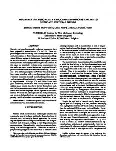
We applied a Gaussian voltage pulse with a magnitude of 3V, standard deviation of .5, and a duration of 3µsec to the left port of the network and observed the induced voltage at the right port. The output is displayed as a solid green trace in Figure 2. The induced response of the linearized network is also displayed as a green dashed line for comparison. Notice that nonlinearity sharpens the peak of the response and significantly reduces dispersion. Notice also that there is a propagation delay in the network of about 0.8µsec. We took 1000 uniformly spaced samples of the system trajectory and internal forcing, applied Algorithm 1 (POD - PH ), and constructed reduced order port-Hamiltonian models of orders r = 6, 12, and 20. We then forced each reduced order model (ROM) with a) the same Gaussian pulse used to generate the POD bases (Figure 2), and b) a positive sinusoid with a peakto-peak magnitude of 3V and frequency of 300kHz (Figure 3). The r = 20 POD - PH model provides the best fidelity for each case, as expected. Lower order models provide coarser

6566

resolution but interestingly, the r = 6 POD - PH model (blue solid line) provides better fidelity for the Gaussian pulse input than what the r = 12 POD - PH model (blue dashed line) is able to provide, especially during the initial lag. This discrepancy is even more pronounced for the sinusoidal input. Notice that for the sinusoidal input, all POD - PH models have some difficulty capturing certain response features such as the initial lag period, the asymmetry of the response peaks, and the response ripple following each peak. /

( +;,5.?;,@.6/!/A?@!>A/B?C/;D"# >?@!>A/B?C/;D#! "

#

$

% & ' +,-./01!2.345627

(

)

*

"!

ROM time response to sinusoid with Gaussian pulse POD basis

respectively. Our model reduction problem reduces to a rational approximation problem: Find a degree-r rational function Gr (s) that approximates G(s) well with respect to an appropriate norm. Here, we focus on interpolatory approaches: Given r interpolation points σ1 , . . . , σr in the complex plane with corresponding tangential directions {b1 , . . . , br } ∈ Cm , the goal is to construct Gr so that Gr not only is portHamiltonian but also tangentially interpolates G, i.e. Gr (σi )bi = G(σi )bi 6567

for i = 1, . . . , r.

(9)

Algorithm 2: QH2 OPT- PH Quasi-optimal reduction of linear port-Hamiltonian systems ([6])

A solution to this problem was recently given in [6] (note that [6] focusses on linear port-Hamiltonian systems): Theorem 1: Given interpolation points σ1 , . . . , σr and tangential directions b1 , . . . , br , construct

1) Make an initial shift selection {σi }r1 , and tangent directions {bi }r1 . 2) while (not converged) b r = [(σ1 I − (J − R)Q)−1 Bb1 , . . . , a) V . . . , (σr I − (J − R)Q)−1 Bbr ]. b r L−1 with V b rT QV b r = LT L b) Set Vr = V (so Qr = VrT QVr = Ir ). c) Set Wr = QVr . (so VrT Wr = Ir ). d) Set Jr = WrT JWr , Rr = WrT RWr , and Br = WrT B. e) Calculate left eigenvectors: zTi (Jr − Rr ) = λi zTi . f) Set σi ←− −λi and bi ←− BTr zi for i = 1, . . . , r 3) Calculate final QH2 OPT- PH bases: b r = [(σ1 I − (J − R)Q)−1 Bb1 , . . . , Find V . . . , (σr I − (J − R)Q)−1 Bbr ]. b r L−1 with V b rT QV b r = LT L. Set Vr = V Set Wr = QVr . 4) With Vr and Wr determined in this way, the QH2 OPT- PH reduced port-Hamiltonian system is then specified by (4).

e r = [(σ1 I − (J − R)Q)−1 Bb1 , . . . , (σr I − (J − R)Q)−1 Bbr ]. V

e r L−1 and Wr = QVr where V e T QV er = Let Vr = V r T L L. Set

Jr = WrT JWr , Qr = VrT QVr = Ir , T Rr = Wr RWr , Br = WrT B.

Then the reduced model, Gr : x˙ r = (Jr − Rr )Qr xr + Br u,

yr = BTr Qr xr

(10)

is port-Hamiltonian, passive, and satisfies the interpolation conditions (9). For information on transfer function interpolation in the special case of single-input/single-output port-Hamiltonian systems, see [9], [5], [10]. For an overview of model reduction methods for linear port-Hamiltonian systems, see [8]. B. Quasi-optimal port-Hamiltonian rational approximation Even though Theorem 1 shows how to construct a structure-preserving interpolatory reduced-order portHamiltonian approximation once {σi } and {bi } are given, it does not give any information on how to choose {σi } and {bi }. We discuss issues related to finding effective approximations with respect to the H2 norm: The H2 norm of G is defined as 1/2  Z ∞ 1 2 kG(ıω)kF dω . kGkH2 = 2π −∞ Let Gr (s) minimize the H2 error kG − Gr kH2 over all possible degree-r rational functions and suppose that Gr (s) Pr c bT has a partial fraction expansion Gr (s) = k=1 k bk . Then, s−λk as shown in [4], the interpolation conditions bk )bk = Gr (−λ bk )bk , G(−λ

for k = 1, . . . , r

(11)

are necessary conditions for H2 optimality (there are additional conditions that must also be satisfied in general). In other words, the optimal H2 approximant Gr is a tangential interpolant to G at the mirror images of the reduced-order poles. For the full set of necessary conditions required for optimality, see [4]. Based on (11), a method was introduced in [6] that produces an interpolatory reduced-order port-Hamiltonian system satisfying the necessary conditions given in (11). bk and the tangential diSince the interpolation points −λ rections bk depend on the reduced-model to be computed, an iterative process is used to correct the interpolation points and tangential directions until the desired conditions in (11) are obtained. A brief sketch of the algorithm is given below in Algorithm 2. We call this method “quasiH2 -optimal” since it only satisfies a subset of the necessary conditions required for optimality. The remaining degrees of freedom are used in maintaining port-Hamiltonian structure. For details, see [6].

We use the linearized port-Hamiltonion model only to obtain the quasi-optimal model reduction subspaces. Once Vr and Wr are obtained using QH2 OPT- PH as outlined in Algorithm 2, we use them to reduce the original nonlinear system as shown in (4). See [?], [?] for other approaches that compute the projection matrices a using a linearized system for reduction of nonlinear systems. C. Example We repeated the same computational experiments on the ladder network described above using instead quasi-H2 optimal subspaces obtained with Algorithm 2. Notice that no simulations are performed and so, unlike POD - PH , the Q H2 OPT- PH subspaces are not tied to any particular input profiles. We applied Algorithm 2, and obtained quasi-H2 -optimal bases of orders r = 6, 12, and 20. We used these subspaces to construct reduced order QH2 OPT- PH port-Hamiltonian models and then performed reduced-order simulations, forcing each ROM with a) the same Gaussian pulse used previously (Figure 4), and b) the same sinusoid used previously (Figure 5). The r = 6 POD - PH results are displayed on the same axes for easy comparison (the r = 12 POD - PH case is omitted since r = 6 POD - PH performed better). The r = 20 QH2 OPT- PH model gave results comparable to the r = 20 POD - PH case (both quite good) and neither is displayed to reduce clutter. The most significant feature that emerges from examination of these results is that the Q H2 OPT- PH models were able to capture response features of true response better at lower order than POD - PH for the two input profiles applied. Notably for the sinusoid input, Q H2 OPT- PH models capture the asymmetry of the response peaks and the response ripple following each peak even at low resolution. All models had some difficulty capturing the initial lag, but the QH2 OPT- PH models generally did

6568

better than the POD - PH models. For the example shown here, Q H2 OPT- PH exhibited generally monotone improvement in fidelity as r increased in sharp contrast with POD - PH on this example. The advantages of QH2 OPT- PH seem most often to occur at low order on signal profiles that did not participate in generation of a POD basis; this was the main motivation to employ input-independent quasi-optimal model reduction techniques. We have presented an example where POD bases can give poor results even with precisely the same signal from which it was generated. /

+;?@!>A/B?C/;D"# E!A ?=:!>A/B?C/;D'

' &

#

E!A#?=:!>A/B?C/;D"#

849:2

%

R EFERENCES

$ # " ! !" / !

"

#

$

%

&

'

(

)

*

"!

+,-./01!2.345627

Fig. 4.

ROM time response to Gaussian pulse using QH2 OPT- PH bases

)

(

/

+;?@!>A/B?C/;D' E!A#?=:!>A/B?C/;D' E!A ?=:!>A/B?C/;D"# #

'

&

849:2

originally targeted for linear port-Hamiltonian systems. Numerical experiments on a nonlinear ladder network illustrate better performance for the latter method, especially with low order approximation and in circumstances where simulations are driven by input profiles that do not participate in the generation of the POD basis. Improving the model reduction subspaces further by combining strengths of both approaches considered here, for example, by selectively merging the two families of subspaces, is the focus of on-going research. Analysis and experimentation of related methods for the fully nonlinear case where J and R themselves carry a dependence on state variables is also under study.

%

$

#

"

!

!" / !

"

#

$

%

&

'

(

)

*

"!

+,-./01!2.345627

Fig. 5.

ROM time response to sinusoid using QH2 OPT- PH bases

IV. C ONCLUSIONS AND F UTURE W ORK We have introduced a structure-preserving projection framework for model reduction of large-scale multiinput/multi-output nonlinear port-Hamiltonian systems leading to reduced-order port-Hamiltonian models. Projecting subspaces are constructed with two different approaches: one is POD-based; the other is related to an H2 -based approach

[1] S. Chaturantabut and D.C. Sorensen. Discrete empirical interpolation for nonlinear model reduction. SIAM J. Sci. Comput, 32(5):2737–2764, 2010. [2] K. Fujimoto and H. Kajiura. Balanced realization and model reduction of port-Hamiltonian systems. In American Control Conference, 2007, pages 930–934, 2007. [3] K. Fujimoto and J.M.A. Scherpen. Balanced realization and model order reduction for nonlinear systems based on singular value analysis. SIAM Journal on Control and Optimization, 48(7):4591–4623, 2010. [4] S. Gugercin, A. C. Antoulas, and C. A. Beattie. H2 model reduction for large-scale linear dynamical systems. SIAM J. Matrix Anal. Appl., 30(2):609–638, 2008. [5] S. Gugercin, R.V. Polyuga, C.A. Beattie, and A.J. van der Schaft. Interpolation-based H2 Model Reduction for port-Hamiltonian Systems. In Proceedings of the Joint 48th IEEE Conference on Decision and Control and 28th Chinese Control Conference, Shanghai, PR China, pages 5362–5369, 2009. [6] S. Gugercin, R.V. Polyuga, C.A. Beattie, and A.J. van der Schaft. Structure-preserving tangential-interpolation based model reduction of port-Hamiltonian systems. Submitted to Automatica, 2011. Available as arXiv:1101.3485v1. [7] K. Kunisch and S. Volkwein. Optimal snapshot location for computing POD basis functions. ESAIM: Mathematical Modelling and Numerical Analysis, 44(3):509–529, 2010. [8] R. V. Polyuga. Model Reduction of Port-Hamiltonian Systems. PhD thesis, University of Groningen, 2010. [9] R. V. Polyuga and A.J. van der Schaft. Structure preserving model reduction of port-Hamiltonian systems by moment matching at infinity. Automatica, 46:665–672, 2010. [10] R. V. Polyuga and A.J. van der Schaft. Structure preserving moment matching for port-Hamiltonian systems: Arnoldi and Lanczos. To appear in IEEE Transactions on Automatic Control, 2010. [11] J.M.A. Scherpen and A.J. van der Schaft. A structure preserving minimal representation of a nonlinear port-Hamiltonian system. In Decision and Control, 2008, 47th IEEE Conference on, pages 4885– 4890, 2008. [12] A.J. van der Schaft. Port-Hamiltonian systems: an introductory survey. In M. Sanz-Sole, J. Soria, J. L. Varona, and J. Verdera, editors, Proceedings of the International Congress of Mathematicians Vol. III, Madrid, pages 1339–1365, Madrid, Spain, 2006. European Mathematical Society Publishing House (EMS Ph). [13] H. Zwart and B. Jacob. Distributed-Parameter Port-Hamiltonian Systems. CIMPA, 2009.

6569