shown in [3] that the optimal (fixed rate) encoder for this case is a function of the current source symbol and the probability mass function of the decoder's state ...
Structure Theorem for Real–Time Variable–Rate Lossy Source Encoders and Memory–Limited Decoders with Side Information Yonatan Kaspi and Neri Merhav Department of Electrical Engineering Technion - Israel Institute of Technology Technion City, Haifa 32000, Israel Email: {kaspi@tx, merhav@ee}.technion.ac.il
Abstract—We extend Witsenhausen’s structure theorem for real–time source coding, so as to accommodate both variable–rate coding and causal side information at the decoder.
I. I NTRODUCTION We consider the following source coding problem. Symbols produced by a discrete Markov source are to be encoded, transmitted noiselessly and reproduced by a decoder which has causal access to side information (SI) correlated to the source. Operation is in real time, that is, the encoding of each symbol and its reproduction by the decoder must be performed without any delay and the distortion measure does not tolerate delays. The decoder is assumed to be a finite state machine with a fixed number of states. With no SI, the scenario where the encoder is of fixed rate was investigated by Witsenhausen [1]. It was shown that for a given decoder, in order to minimize the distortion at each stage for a Markov source of order k, an optimal encoder can be sought among those for which the encoding function depends on the k last source symbols and the decoder’s state (in contrast to the general case where its a function of all past source symbols). The scenario where the encoder is also a finite state machine was considered by Gaarder and Slepian in [2]. In [3], Teneketzis considered the case where there is a noisy channel between the encoder and decoder. In this case, unlike this work and [1],[2], the encoder cannot track the decoder’s state. It is shown in [3] that the optimal (fixed rate) encoder for this case is a function of the current source symbol and the probability mass function of the decoder’s state for the symbols sent so far. When the time horizon and alphabets are finite, there is a finite number of possible encoding, decoding and memory update rules. Theoretically, a brute force search will yield the optimal choice. However, since the number of possibilities increases doubly exponentially in the duration of the communication and exponentially in the alphabet size, it is not trackable even for very short time horizons. Recently, using the results of [3], Mahajan and Teneketzis [4], proposed a search frame that is linear in the communication length and doubly exponential in the alphabet size. Real time codes are a subclass of causal codes, as defined
by Neuhoff and Gilbert [5]. In [5], entropy coding is used on the whole sequence of reproduction symbols, introducing arbitrarily long delays. In the real time case, entropy coding has to be instantaneous, symbol by symbol (possibly taking into account past transmitted symbols). It was shown in [5], that for a discrete memoryless source (DMS), the optimal causal encoder consists of time–sharing between no more than two memoryless encoders. Weissman and Merhav [6], extended [5] to the case where SI is also available at the decoder, encoder or both. Error exponents for real time coding with finite memory for a DMS where derived in [7]. This work extends [1] in two directions: The first direction is from fixed–rate coding to variable–rate coding, where accordingly, the cost function is redefined so as to incorporate both the expected distortion and the expected coding rate. The second direction of extension is in allowing the decoder access to causal side information. Our main result is that a structure theorem, similar to that of Witsenhausen [1], continues to hold in this setting as well. As mentioned in the previous paragraph, in contrast to [1]–[3], where fixed–rate coding was considered, and hence the performance measure was just the expected distortion, here, since we allow variable–rate coding, our cost function incorporates both rate and distortion. This is done by defining our cost function in terms of the Lagrangian (distortion) + λ · (code length). In [1], the proof of the structure theorem relied on two lemmas. The proof of the extension of those lemmas to our case is more involved than the proofs of their respective original versions in [1]. To intuitively see why, remember that the proof of the lemmas in [1], relied on the fact that for every decoder state, source symbol and a given decoder, since there is a finite number of possible encoder outputs (governed by the fixed rate), we could choose the one minimizing the distortion. However, in our case, such a choice might entail a large expected coding rate, and although minimizes the distortion, it will not minimize the overall cost function (especially for large λ).
The remainder of the paper is organized as follows: In Section II, we give the formal setting and notation used throughout the paper. In Section III, we state and prove the main result of this paper. Finally, we conclude this work in Section IV. II. P RELIMINARIES We begin with notation conventions. Capital letters represent scalar random variables (RV), specific realizations of them are denoted by the corresponding lower case letters and their alphabet – by calligraphic letters. For i < j (i, j positive integers), xji will denote the vector (xi , . . . , xj ), where for i = 1 the subscript will be omitted. We consider a k-th order Markov source, producing a random sequence X1 , X2 , ..., XT , Xt ∈ X , t = 1, 2, . . . , T . The cardinality of X , as well as other alphabets in the sequel, is finite. The SI sequence, W1 , W2 , ..., WT , Wt ∈ W, is generated by a discrete memoryless channel (DMC), fed by X1 , X2 , . . . , XT : P (W1 , . . . , WT |X1 , . . . XT ) =
T Y
P (Wt |Xt ).
(1)
t=1
The probability mass function of X1 , P (X1 ) and the transition probabilities, denoted by t−1 P (X2 |X1 ),P (X3 |X 2 ),...,P (Xt |Xt−k ), t = k +1, k +2, . . . , T are known. A variable length encoder is a sequence of T functions {ft }t=1 . At stage t, an encoder ft : X t → Yt calculates Yt = ft (X t ) and noiselessly transmits an entropy coded codeword of Yt . Yt ⊆ Y is the alphabet used at stage t. Unlike the fixed rate regime in [1],[3], where log2 |Yt | (rounded up) was the rate of the code of stage t, here the size of the codebook will be one of the outcomes of the optimization. The encoder structure is not confined a–priori, and it is not even limited to be deterministic: at each time instant t, Yt may be given by an arbitrary (possibly stochastic) function of X t . The decoder, however, is assumed, similarly as in [1] and [3], to be a finite–memory device, defined as follows: At each stage, t, the decoder updates its current state (or memory) ˆ t . We assume that the and outputs a reproduction symbol X decoder’s state can be divided into two parts. Ztw ∈ Z w is updated by: Z1w = r1w (W1 , Y1 ) w Ztw = rtw (Wt , Yt , Zt−1 ),
t = 2, 3, . . . , T
(2)
y∈Yt
The average codeword length of stage t will be given by: X X 4 y P (y|z)l(y) . (6) L(Yt |Zt−1 )= P (z) min l(·)∈At y y∈Yt
z∈Z
y ) will denote the optimal average codeword length L(Yt |zt−1 y y ) is . L(Yt |zt−1 at stage t, for a specific decoder state, zt−1 obtained by designing a Huffman code for the probability y distribution P (·|zt−1 ). The model is depicted in Figure 1.
Encoder Xt
ft ( X t )
Yt
Decoder y
Entropy Coder
L (Yt | Z t −1 ) bits
Entropy Decoder
Yt
Reproduction Function
Xˆ t
P (W | X )
Fig. 1: System model T
We are given a sequence of distortion measures {ρt }t=1 , ρt : X × Xˆ → IR+ . At each stage, the cost function is a linear combination of the average distortion and codeword length y L(Yt |Zt−1 ), i.e. n o 4 ˆ t ) + λL(Yt |Z y ). D(t) = E ρt (Xt , X t−1
(7)
where λ is a fixed parameter that controls the tradeoff between rate and distortion. Our goal is to minimize the cumulative cost 4
D=
and Zty ∈ Z y is updated by
T X
D(t).
(8)
t=1
Z1y = r1y (Y1 ) y ), Zty = rty (Yt , Zt−1
y is known to both Since at the beginning of stage t, Zt−1 encoder and decoder, the entropy coder at every stage needs y to encode the random variable Yt given Zt−1 . We define At to be the set of all uniquely decodable codes for Yt , i.e all possible length functions l : Yt → Z + that satisfy Kraft’s inequality: X At = l(·) : 2−l(y) ≤ 1 (5)
t = 2, 3, . . . , T
(3)
Both parts depend on the received compressed data Yt . However, since Zty does not depend on the SI and the transmission is noiseless, it can be tracked by the encoder. The reproduction symbols are produced by a sequence of functions {gt }, gt : Y × W × Z w × Z y → Xˆ as follows ˆ 1 = g1 (W1 , Y1 ) X y w ˆ t = gt (Wt , Yt , Zt−1 X , Zt−1 ),
t = 2, 3, . . . , T
(4)
A specific choice of the memory update functions {rty },{rtw } reproduction functions {gt } and encoders {ft } along with their resulting cost D is called a design. We say that design A with cumulative cost DA outperforms design B, with cumulative cost DB , if DA ≤ DB . We say that the encoder has memory order k if Yt is produced using the decoder’s state that is tracked by the encoder and the last k source symbols, y t i.e Yt = ft (Xt−k+1 , Zt−1 ). In the following section, we state and prove a structure theorem for the system described above.
III. M AIN R ESULT The main result of this paper is the following theorem: Theorem 1. Under the conditions described in Section II, for any given design of the system, there exists a design with the same decoders, whose encoders are deterministic and have memory order k, that outperforms the original design. Remark: We will prove this structure theorem using lemmas regarding the structure of a two and three stage system (T = 2, 3) and then use backwards induction as we show in the following subsections. This is the original method used by Witsenhausen [1]. The main difference is in the proofs of the lemmas, which call for more caution. In [1], these lemmas could be proved by optimizing the encoder over the distortion y ). For function independently for each possible pair (xi , zi−1 each such pair, Yt was chosen as the one that minimizes y the distortion ρt (Xt , gt (Yt , Zt−1 )). Here, even without SI, we cant take this approach since such Yt (that minimizes the distortion) might entail a large L(Yt |Zt−1 ). Moreover, y Yt |Zt−1 , is well defined only after all stage t encoding rules y are known. Any change for a specific (xi , zi−1 ) will affect the y PMF of Yt |Zt−1 (and the code length) and therefore cannot be done independently of the other pairs. We start by stating and proving the lemmas for the two and three stage systems in the next two subsections. Using these lemmas, Theorem 1 is proved in Section III-C A. Two stage lemma Lemma 1. For a two stage system (T = 2), any source, SI sequence and any given design, a design different only in f2 , with f2 deterministic and having memory order of k = 1, will outperform the original design. f1 , g1 , g2 , r1y , r1w
Proof: Note that are fixed and D(1) is unchanged by changing f2 . We need to show that f2 that minimizes D(2) can be a deterministic function of X2 , Z1y . For every joint probability measure over the 6–tuple (X1 , X2 , W2 , Y2 , Z1w , Z1y ), D(2) is well defined and our goal is to minimize: D(2) = E {ρ2 (X2 , g2 (W2 , Y2 , Z1w , Z1y ))} + λL(Y2 |Z1y ) (9) with respect to the second stage encoder. Note that the expectation is over (X1 , X2 , W2 , Y2 , Z1w , Z1y ) in the first expression only. The second expression (which is a constant) contains the expectation in its definition. Let us look at the 6–tuple of RV’s (X1 , X2 , W2 , Y2 , Z1w , Z1y ). From the structure of the system we know that P (X1 , X2 , W2 , Y2 , Z1w , Z1y ) = P (X1 )P (X2 |X1 )P (Y1 |X1 )× P (Z1y |X1 )P (Z1w |X1 )P (Y2 |X1 , X2 )P (W2 |X2 )
(10)
Everything but the second stage encoder P (Y2 |X1 , X2 ) is fixed. Our objective is to find min
P (Y2 |X1 ,X2 )
E {ρ2 (X2 , g2 (W2 , Y2 , Z1w , Z1y ))} + λL(Y2 |Z1y ) (11)
Note that the minimization affects L(Y2 |Z1y ) since its inner minimization depends on P (Y2 |Z1y ) which in turn depends on P (Y2 |X1 , X2 ). We rewrite the expression in (11): Eρ2 (X2 , g2 (W2 , Y2 , Z1w , Z1y )) + λL(Y2 |Z1y ) X min P (x1 , x2 , w2 , y2 , z1w , z1y )×
min
P (Y2 |X1 ,X2 )
=
P (Y2 |X1 ,X2 )
x1 ,x2 ,w2 ,y2 ,z1w ,z1y {ρ2 (x2 , g2 (w2 , y2 , z1w , z1y )) + λL(Y2 |z1y } .
(12)
For any P (Y2 |X1 , X2 ) and given z1y , L(Y2 |z1y ) does not depend on x1 and obviously, ρ2 (x2 , g2 (w2 , y2 , z1w , z1y )) is not a function of x1 . Therefore the term in brackets does not depend on x1 . Define 4
d02 (x2 , y2 , z1w , z1y ) = " # X w y P (w2 |x2 )ρ2 (x2 , g2 (w2 , y2 , z1 , z1 )) + λL(Y2 |z1y ) w2
(13) Also note that z1y , z1w does not play a role in the optimization. Therefore, min X
P (Y2 |X1 ,X2 )
=
z1w ,z1y
Eρ2 (X2 , g2 (W2 , Y2 , Z1w , Z1y )) + λL(Y2 |Z1y ) X min P (x2 , y2 , z1w , z1y )d02 (x2 , y2 , z1w , z1y )
P (Y2 |X1 ,X2 )
x2 ,y2
(14) Now, given that the first stage encoder and decoder are known, P (x2 , z1w , z1y ) is well defined. Also, since the encoder does not have access to the side information sequence, we have, for any second stage encoder: P (X2 , Y2 , Z1w , Z1y ) = P (Y2 |X2 , Z1y )P (X2 , Z1w , Z1y )
(15)
For a given z1y and any second stage encoder, L(Y2 |z1y ) is given by X X P (x2 , z w , z y ) 1 1 P (y2 |x2 , z1y )l(y2 ) L(Y2 |z1y ) = min y P (z ) l(y2 )∈At w 1 y x ,z 2
2
1
(16) Substituting (15)–(16) back into (14) we have Eρ2 (X2 , g2 (W2 , Y2 , Z1w , Z1y )) + λL(Y2 |Z1y ) (� X X w y = P (z1 , z1 ) min P (x2 , z1w , z1y )× min
P (Y2 |X1 ,X2 )
P (Y2 |X1 ,X2 )
z1w ,z1y
X
x2
P (y2 |x2 , z1y )ρ2 (x2 , g2 (w2 , y2 , z1w , z1y ))
�
y2
) + λ min
l∈At
X
P (y20 |x02 , z1y )P (x2 , z1w |z1y )l(y20 )
(17)
y20 ,x02
Note that, for any P (Y2 |X2 , Z1y ), there can be more than one possible second stage encoder which will yield the same r.h.s in (15) (there is at least one such encoder: P (y2 |x1 , x2 ) = P (y2 |x2 , z1y ) for all x1 with P (z1y , x1 ) > 0 for all x2 , y2 , z1y ).
However, from (17), it is clear that all second stage encoders that result in the same marginal P (Y2 |X2 , Z1y ) will yield the same second stage average cost D(2). Now, every possible P (Y2 |X2 , Z1y ) has at least one possible P (Y2 |X1 , X2 ) that leads to it. Since every P (Y2 |X1 , X2 ) results in some P (Y2 |X2 , Z1y ), minimizing over P (Y2 |X2 , Z1y ) will yield the same (optimal) cost function for the second stage. Therefore, we have min
P (Y2 |X1 ,X2 )
=
min
Eρ2 (X2 , g2 (W2 , Y2 , Z1w , Z1y )) + λL(Y2 |Z1y )
P (Y2 |X2 ,Z1y )
Eρ2 (X2 , g2 (W2 , Y2 , Z1w , Z1y ))
+
λL(Y2 |Z1y ) (18)
and we showed that its enough to search for second stage encoding rules that depend only on X2 , Z1y and still receive the optimal second stage cost. Now, since L(Y2 |Z1y ) is a concave functional of P (Y2 |X2 , Z1y ) (see Appendix), the second stage cost function is concave in P (Y2 |X2 , Z1y ). This means that the minimizing P (Y2 |X2 , Z1y ) is one of the extreme points of the simplex consisting of all possible P (Y2 |X2 , Z1y ). Since the extreme points of the simplex represent a deterministic choice of y2 given x2 , z1y , this means that an optimal second stage encoder is a deterministic function of (X2 , Z1y ). B. Three stage lemma Lemma 2. For a three stage system (T = 3), first order Markov source and SI as described in Section II, any design in which f3 has memory order of k = 1 will be outperformed by a design different only in f2 , where f2 in the new design is deterministic and with memory order of k = 1. Proof: The first stage encoder and decoder, and therefore the first stage cost, are fixed. We optimize the second stage encoder given a decoder and a memory update function. The minimum cost of the last two stages is given by the minimization of: D(2) + D(3) = E {ρ2 (X2 , g2 (W2 , Y2 , Z1w , Z1y )) +λL(Y2 |Z1y ) + ρ3 (X3 , g3 (W3 , Y3 , Z2w , Z2y )) +λL(Y3 |Z2y )}
(19)
with respect to P (Y2 |X1 , X2 ). Since we know the second stage decoder and the third stage encoder/decoder pair P (X3 , W3 , Y3 , Z2w , Z2y |X2 , W2 , Y2 , Z1w , Z1y )
(20)
is well defined regardless of the second stage encoder. Therefore we can calculate the conditional expectation of the third stage cost given X2 , W2 , Y2 , Z1w , Z1y . 4
d3 (x2 , w2 , y2 , z1w , z1y ) = X P (x3 , w3 , z2w , z2y |x2 , w2 , y2 , z1w , z1y )×
P (Y2 |X1 ,X2 )
×
x1 ,x2 ,y2 ,z1w ,z1y {ρ2 (x2 , g2 (w2 , y2 , z1w , z1y )) + λL(Y2 |z1y ) +d3 (x2 , w2 , y2 , z1w , z1y )}
(21)
Here, when we wrote P (X3 |X2 ), we used the fact that the source is Markov. This, alongside the requirement that the
(22)
Let ρ02 (x2 , y2 , z1w , z1y ) = ρ2 (x2 , g2 (w2 , y2 , z1w , z1y )) + d3 (x2 , w2 , y2 , z1w , z1y ).
(23)
Substituting this into (22) and using the fact that, as in the two stage lemma case, given x2 , z1w , z1y , the term in brackets in (22) is not a function of x1 we have X D(2) + D(3) = min P (x2 , y2 , z1w , z1y )× P (Y2 |X1 ,X2 )
{ρ02 (x2 , y2 , z1w , z1y )
x2 ,y2 ,z1w ,z1y + λL(Y2 |z1y )}
(24)
Note the similarity of the last expression to (12). Although here we have a different distortion measure, both here and in (12) the distortion measures are functions on x2 , y2 , z1w , z1y . Therefore, the same steps we used to prove the two stage lemma after (12), can be used here and the three stage lemma will be proven. Remark: From looking back at the definition of d3 (x2 , w2 , y2 , z1w , z1y ) in (21), it is clear that the three stage lemma will continue to hold if the third stage encoder would have memory order of k = 2, since the resulting conditional expectation in (21) still would not be a function of x1 . However, this is not needed in the proof of Theorem 1. C. Proof of Theorem 1 With the two and three stage lemmas, we can prove Theorem 1 by using the method of [1], used for fixed rate encoding. We will prove Theorem 1 for a first order Markov source. The extension to a k-th order Markov source is straight forward by repacking k source symbols each time into a ˆt = new super symbol in a “sliding window” manner: X (Xt , Xt+1 , . . . , Xt+k−1 ). The SI is produced from these super symbols. The resulting source (with super symbols) is a first order Markov source for which the proof we give here can be applied. An encoder with memory order k = 1 with the super symbols has memory order k with the original source. We need one last auxiliary lemma before we can prove Theorem 1. Lemma 3. For any source statistics, SI and any design, one can replace the last encoder, fT , with a deterministic encoder having memory order k = 1 and the new design will outperform the original design. 0
x3 ,w3 ,z2w ,z2y
{ρ3 (x3 , g3 (w3 , y3 , z2w , z2y )) + λL(Y3 |z2y )}
third stage encoder has memory order of k = 1, ensures that d3 (x2 , w2 , y2 , z1w , z1y ) is not a function of x1 . We rewrite (19): X D(2) + D(3) = min P (x1 , x2 , y2 , z1w , z1y )
0
Proof: Let X1 = X T −1 , W1 = W T −1 . We now have a two 0 0 stage system with source symbols (X1 , XT ) and SI (W1 , WT ). Now, by the the two stage lemma, the second stage encoder in the new two stage system. has memory order k = 1 for any first stage encoding and decoding rules.
The main theorem is proven by backward induction. First apply the last lemma to any design to conclude that an optimal fT has memory order k = 1. Now assume that the last m encoders (i.e fT −m+1 , ..., fT ) have memory order k = 1. We will show that the encoder at time T −m also has this structure and continue backwards until t = 2. The first encoder, trivially, has memory order k = 1. To prove the induction step, define ˆ 1 = (X1 , X2 , ..., XT −m−1 ) X ˆ 1 = (W1 , W2 , ..., WT −m−1 ) W Yˆ1 = (Y1 , Y2 , ..., YT −m−1 ) Zˆ1w Zˆ1y
= =
= =
=
for some 0 ≤ α ≤ 1. Focusing on the inner minimization of the definition of L(Y2 |Z1y ) (see (6)) we have � X
P (y2 |z1y )l(y2 )
�
y2 ∈Y
= min
� X X
l(·)∈A2
[αP1 (y2 |x2 , z1y )
y2 ∈Y x2 ∈X
� + (1 − α)P2 (y2 |x2 , z1y )] P (x2 |z1y )l(y2 ) � X X � y y ≥ α min P1 (y2 |x2 , z1 )P (x2 |z1 )l(y2 ) l(·)∈A2
rTw−m (WT −m , YT −m , ZTw−m−1 ) rTy −m (YT −m , ZTw−m−1 )
y2 ∈Y x2 ∈X
� X X
+ (1 − α) min l(·)∈A2
P2 (y2 |x2 , z1y )P (x2 |z1y )l(y2 )
�
y2 ∈Y x2 ∈X
(27) LP (Y2 |Z1y ),
(25)
where rˆ1y (Yˆ1 )
P (Y2 |X2 , Z1y ) = αP1 (Y2 |X2 , Z1y ) + (1 − α)P2 (Y2 |X2 , Z1y )
l(·)∈A2
ˆ 1) rˆ1w (Yˆ1 , W y ˆ rˆ1 (Y1 )
ˆ 3 = (XT −m+1 , XT −m+2 , ..., XT ) X ˆ 3 = (WT −m+1 , WT −m+2 , ..., WT ) W Yˆ3 = (YT −m+1 , YT −m+2 , ..., YT )
This appendix show that L(Y2 |Z1y ) is concave in P (Y2 |X2 , Z1y ). Let
min
ˆ 2 = XT −m X ˆ 2 = WT −m W Yˆ2 = YT −m Zˆ2w Zˆ2y
A PPENDIX
rTy −m−1 (YT −m−1 , rTy −m−2 (. . . r2y (Y2 , r1y Y1 )) . . .) (26)
and is defined likewise. In words, Zˆ1w , Zˆ1y are the states of the decoder after T − m − 1 stages. Using this new notation, the encoder that produces Yˆ3 has ˆ 3 , Zˆ y memory order of k = 1, since its a function of X 2 (since, by assumption, the last m encoders in the original notation are of memory order of k = 1). The source is ˆ 3 is independent of X ˆ 1 given X ˆ 2 (since the Markov since X original source is Markov). Now, by the three stage lemma, ˆ 2 , Zˆ y ) = fT −m (XT −m , Z y Yˆ2 = YT −m = fT −m (X 1 T −m−1 ). Thus, the induction step is proved. ˆ 1) rˆ1w (Yˆ1 , W
IV. C ONCLUSIONS We showed that the results of [1] can be extended to both include variable rate coding and SI at the decoder. Following the same steps we used, this result can be further extended to the case the decoder has SI with some lookahead (i.e at time t it sees Wtt+l where l is the lookahead). The results of [1] and some of the results in [3] are obtained in the special case of λ = 0, i.e the instantaneous rate is not taken into account in the cost function if we set Yt to be the encoder output alphabet size at stage t of [1].
LP1 (Y2 |Z1y ),
LP2 (Y2 |Z1y ) denote the length P (Y2 |X2 , Z1y ), P1 (Y2 |X2 , Z1y ),
Let function calculated with P2 (Y2 |X2 , Z1y ) respectively. Substituting this into the definition of L(Y2 |Z1y ) we have: LP (Y2 |Z1y ) ≥ αLP1 (Y2 |Z1y ) + (1 − α)LP2 (Y2 |Z1y )
(28)
R EFERENCES [1] H. S. Witsenhausen, “The structure of real time source coders,” Bell Systems Technical Journal, vol. 58, no. 6, pp. 1338–1451, July 1979. [2] N. T. Gaarder and D. Slepian, “On optimal finite-state digital transmission systems,” IEEE Transactions on Information Theory, vol. 28, no. 3, pp. 167–186, March 1982. [3] D. Teneketzis, “On the structure of optimal real-time encoders and decoders in noisy communication,” IEEE Transactions on Information Theory, vol. 52, no. 9, pp. 4017–4035, September 2006. [4] A. Mahajan and D. Teneketzis, “Optimal design of sequential real-time communication systems,” IEEE Transactions on Information Theory, vol. 55, no. 11, pp. 5317–5338, November 2009. [5] D. Neuhoff and R. K. Gilbert, “Causal source codes,” IEEE Transactions on Information Theory, vol. 28, no. 5, pp. 701–713, September 1982. [6] T. Weissman and N. Merhav, “On causal source codes with side information,” IEEE Transactions on Information Theory, vol. 51, no. 11, pp. 4003–4013, November 2005. [7] N. Merhav and I. Kontoyiannis, “Source coding exponents for zero-delay coding with finite memory,” IEEE Transactions on Information Theory, vol. 49, no. 3, pp. 609–625, March 2003.