Diversity-induced Multi-view Subspace Clustering Xiaochun Cao1,2 Changqing Zhang1 Huazhu Fu3 Si Liu2 Hua Zhang1 1 School of Computer Science and Technology, Tianjin University, Tianjin 300072, China 2 State Key Laboratory of Information Security, IIE, Chinese Academy of Sciences, Beijing, 100093, China 3 School of Computer Engineering, Nanyang Technological University, Nanyang Avenue 639798, Singapore
[email protected]
[email protected]
[email protected]
Abstract In this paper, we focus on how to boost the multi-view clustering by exploring the complementary information among multi-view features. A multi-view clustering framework, called Diversity-induced Multi-view Subspace Clustering (DiMSC), is proposed for this task. In our method, we extend the existing subspace clustering into the multi-view domain, and utilize the Hilbert Schmidt Independence Criterion (HSIC) as a diversity term to explore the complementarity of multi-view representations, which could be solved efficiently by using the alternating minimizing optimization. Compared to other multi-view clustering methods, the enhanced complementarity reduces the redundancy between the multi-view representations, and improves the accuracy of the clustering results. Experiments on both image and video face clustering well demonstrate that the proposed method outperforms the state-of-the-art methods.
1. Introduction Multi-view data are very common in many real world applications because data is often collected from diverse domains or obtained from different feature extractors. For example, color and texture information can be utilized as different kinds of features in images and videos. Web pages are also able to be represented using the multi-view features based on text and hyperlinks. Taken alone, these views will often be deficient or incomplete because different views describe distinct perspectives of data. Therefore, a key problem for data analysis is how to integrate the multiple views and discover the underlying structures. Recently, some approaches of learning from multi-view data have been proposed. However, most of them concentrate on supervised or semi-supervised learning [1, 6, 22, 31], in which a validation set is required. In this paper, we focus on multiview clustering, which is much more challenging for lacking training information to guide the learning process. The complementary principle of multi-view setting s-
[email protected]
[email protected]
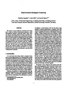
tates that, each view of the data may contain some knowledge that other views do not have. Therefore, multiple views can be employed to comprehensively and accurately describe the data [30, 31]. Furthermore, some theoretical results [4, 5, 26] have shown that the independence of different views can serve as a helpful complement to the multi-view learning. Nevertheless, the main limitation of the existing methods [8, 9, 12, 16, 17, 24, 25] is that they could not guarantee the complementarity across different similarity matrices corresponding to different views. In other words, they assume that the complementary information is abundant across the independently constructed similarity matrices or the views are sufficiently independent to each other. However, we find that exploiting the specific independently constructed matrices is insufficient, and exploring the underlying complementarity is of great importance for the success of multi-view clustering. Figure 1(a-c) illustrates the straightforward way to combine the multi-view features, which independently constructs the similarity matrix of each feature according to some specific distance metric. By contrast, we consider the complementary information of all the different views in depth, and find that the complementary information is explored more thoroughly, while the similarity matrices of the multi-view features are more diverse. In this paper, a novel multi-view subspace clustering method, called Diversityinduced Multi-view Subspace Clustering (DiMSC), is proposed to explore the complementary information. As shown in Figure 1(d-f), our method learns all the different subspace representations jointly with the help of the diversity constraint. The Hilbert-Schmidt Independence Criterion (HSIC) is employed to measure dependence in terms of a kernel dependence measure. With this term, we explicitly co-regularize different views to enforce the diversity of the jointly learned subspace representations. The main contribution of our work is that we extend the self-representation based subspace clustering to multiview setting, and propose a Diversity-induced Multi-view Subspace Clustering method, which outperforms the related
(1) NaMSC
(2) DiMSC
X(1)(GABOR)
X (1)(GABOR) Z
(1)
X (V) (LBP)
Z(1)
X(V) (LBP) Z(V)
Z(V)
(a) Multi-view Data (b) Non-diverse Representations (c) Clustering Result
(d) Multi-view Data
(e) Diverse Representations
(f) Clustering Result
Figure 1. Comparison of naive multi-view subspace clustering (NaMSC) and our DiMSC. The green rectangle indicates the ground-truth clustering. With the multi-view input (a), NaMSC independently learns the subspace representations using SMR [15] (b), which can not ensure the complementarity across different views. In contrast, our DiMSC employs diverse subspace representations to explore the complementary information across the multiple views, and the final clustering result (f) is obtained.
state-of-the-art methods in handling multi-view data. Moreover, we introduce a novel scheme to ensure the diversity of different subspace representations based on HSIC. With the inner product kernel for HSIC, our formulation is simple to resolve and theoretically guaranteed to convergence.
2. Related Work Most existing multi-view clustering methods exploit the multi-view features with graph-based models. For example, the work in [9] constructs a bipartite graph to connect the two-view features, and uses a standard spectral clustering to obtain the 2-view clustering result. The approach in [24] fuses the information from multiple graphs with Linked Matrix Factorization, where each graph is approximated by matrix factorization with a graph-specific factor and a factor common to all graphs. The approaches in [17], [25] co-regularize the clustering hypotheses to exploit the complementary information within the spectral clustering framework. In [16], a co-training based framework is proposed where it searches for the clusterings that agree across the different views. In Multiple Kernel Learning (MKL), as suggested in earlier work [8], even simply combining different kernels by adding them often leads to near optimal results as compared to more sophisticated approaches for classification. Instead of equally adding these kernels, views are expressed in terms of given kernel matrices and a weighted combination of these kernels is learned in parallel to the partitioning in [12]. Note that, the similarity matrices in these methods are independently constructed, while our DiMSC constructs the similarity matrices jointly aiming to promote the complementarity across different views. Recently, the subspace clustering methods have been proposed to explore the relationships between samples with self-representation (e.g., sparse subspace clustering (SSC) [10], low-rank representation segmentation (LRR) [18] and
smooth representation clustering (SMR) [15]), and be employed in numerous research areas, including face clustering [29, 32], image segmentation[7], and medical image analysis [11]. However, these methods only consider the single view feature, where the similarity matrix is constructed based on these reconstruction coefficients. The work in [14] formulates the subspace learning with multiple views as a joint optimization problem with a common subspace representation matrix and a group sparsity inducing norm. The work in [27] provides a convex reformulation of 2-view subspace learning. There are some methods based on dimensionality reduction, which usually learn a low-dimensional subspace from the multiple views and then apply any existing clustering method to get the result. The representative methods in this stream are proposed in [3, 5], which use canonical correlation analysis (CCA) to project the multi-view high dimensional data onto a lowdimensional subspace. Most of these methods do not consider enforcing the complementarity of different views. Although the method [27] enforces conditional independence to guarantee the complementarity while reducing dimensionality, it can only be applied for 2-view setting. In contrast, we enforce the complementarity by directly enhancing the dependence of different views and is not limited to the number of views.
3. The Proposed Method 3.1. Naive Multi-view Subspace Clustering Suppose X = [x1 , x2 , ..., xn ] ∈ Rd×n is the matrix of data vectors, where each column is a sample vector and d is the dimensionality of the feature space. To cluster the data into their respective subspaces, we need to compute an similarity matrix that encodes the pairwise similarity between data pairs. Thus, the self-representation manner is written
mulation by minimizing:
in a compact matrix form: X = XZ + E,
(1)
where Z = [z1 , z2 , ..., zn ] ∈ Rn×n is the coefficient matrix with each zi being the new representation of sample xi , and E is the error matrix. After obtaining the self-representation matrix Z, the similarity matrix S is usually constructed as [10]: (2) S = |Z| + |ZT |, where | · | denotes the absolute operator. Afterwards, the similarity matrix is used as the input of spectral clustering algorithm [19] to obtain the final clustering result. The subspace based clustering technique has shown its power in many image processing fields. However, the multi-view representation is ubiquitous and, hence, extending subspace clustering into the multi-view setting is of vital importance for many applications. In this paper, we firstly introduce a simple and direct way to extend the single-view subspace clustering to multiview setting. As in SMR, we employ the graph regularization technique, which explicitly enforces the subspace representation to meet the grouping effect [15]. We use X(v) to denote the feature matrix corresponding to the v th view. Similarly, we use Z(v) to denote the learned subspace representation corresponding to the v th view. We (v) use xij to denote the entry of X(v) at the ith row and j th column. Specifically, a pair of points should be close to each other in new representation if they are close in the original feature space. Formally, it has the following form: ||xi − xj ||2 → 0 ⇒ ||zi − zj ||2 → 0, ∀i 6= j. Therefore, the objective function of smooth representation clustering corresponding to the v th view turns out to be: min f (Z(v) ) = ||X(v) − X(v) Z(v) ||2F + α(v) Ω(Z(v) ), Z(v)
(3) where α(v) are tradeoff factors and Ω(·) denotes the smooth regularized term which is defined as follow: n
Ω(Z(v) ) =
n
1 X X (v) (v) (v) w ||zi − zj ||22 2 i=1 j=1 ij (v) T
= tr(Z(v) L(v) Z
V X O(Z(1) , .., Z(V ) ) = ||X(v) − X(v) Z(v) ||2F v=1
+
(5) α
(v)
tr(Z
(v)
(v)
L
(v) T
Z
),
v=1
where V is the number of all views. This method learns each subspace representation independently. Therefore, it cannot ensure the complementarity of different views. We call the method Naive Multi-view Subspace Clustering (NaMSC).
3.2. Diversity-induced Multi-view Subspace Clustering According to the objective function (5), NaMSC only combines multi-view representations directly, without any constraint. Here, we explore the complementary information across different views by enforcing the diversity of all representations. High independence means high diversity of two variables [20, 21]. Classical independence criteria include Spearmans rho and Kendalls tau, which can detect only linear dependencies. We employ the Hilbert-Schmidt Independence Criterion (HSIC) to measure the dependence of variables for several reasons. First, HSIC measures dependence by mapping variables into a reproducing kernel Hilbert space (RKHS) such that correlations measured in that space correspond to high-order joint moments between the original distributions and more complicated (such as nonlinear) dependence can be addressed. Second, this approach is able to estimate dependence between variables without explicitly estimating the joint distribution of the random variables. Hence, it is of high computational efficiency. Last but not least, the empirical HSIC turns out to be equal to the trace of product of the data matrix, which makes our problem solvable. Our goal is to promote the diversity of subspace representations, and thus we employ the HSIC to penalize for dependence between data in two representations. Specifically, to ensure that one representation is novel compared to another, we use HSIC to penalize for dependence between data in the two representations.
(4) 3.2.1
), (v)
V X
where tr denotes the matrix trace. W(v) = (wij ) is the weight matrix measuring the spatial closeness of points. L(v) = D(v) − W(v) is the Laplacian matrix, in which Pn (v) (v) D(v) is the diagonal degree matrix with dii = j=1 wij . There are lots of ways to construct W(v) . In this paper, we employ the inner product to measure the similarity, since it is simple to implement and it performs well in practice. Then, we have an naive multi-view subspace clustering for-
Representation Diversity Term
First, we recall the definition of cross-covariance Cxy . Let us define a mapping φ(x) from x ∈ X to kernel space F, such that the inner product between vectors in that space is given by a kernel function k1 (xi , xj ) =< φ(xi ), φ(xj ) >. Let G be a second kernel space on Y, with kernel function k2 (yi , yj ) =< ϕ(yi ), ϕ(yj ) >. The cross-covariance is a function that gives the covariance of two random variables and defined as follow: Cxy = Exy [(φ(x) − µx ) ⊗ (ϕ(y) − µy )].
(6)
where µx = E(φ(x)) and µy = E(ϕ(y)), and ⊗ is the tensor product. Then, we have the following definition of HSIC [13]: Definition 3.1. Given two separable RKHSs F, G and a joint distribution pxy , we define the HSIC as the HilbertSchmidt norm of the associated cross-covariance operator Cxy : HSIC(pxy , F, G) := ||Cxy ||2HS , (7) where ||A||HS denotes the Hilbert-Schmidt norm of a matrix as: sX (8) a2ij . ||A||HS = i,j
However, the joint distribution pxy is often unknown or hard to estimate. Thus, the empirical version of HSIC is induced as follow:
enforce that the learned subspace representations to meet the grouping effect independently and diversity jointly. Our method is not limited to one specific subspace clustering method. Our method is based on SMR because SMR is the state-of-the-art method. Nevertheless, the other subspace clustering algorithms, such as SSC, LRR can also be implemented into our method.
3.3. Solving the Optimization Problem With the alternating minimizing strategy, we can approximately solve equation (10) in the manner of minimizing with respect to one view once at a time while fixing the other views. Specifically, with all but one Z(v) fixed, we minimize the following objective function: F(Z(v) ) = ||X(v) − X(v) Z(v) ||2F T
Definition 3.2. Consider a series of n independent observations drawn from pxy , Z := {(x1 , y1 ), ..., (xn , yn )} ⊆ X × Y, an estimator of HSIC, written as HSIC(Z, F, G), is given by: HSIC(Z, F, G) = (n − 1)−2 tr(K1 HK2 H),
(9)
where K1 and K2 are the Gram matrices with k1,ij = k1 (xi , xj ), k2,ij = k2 (yi , yj ). hij = δij − 1/n centers the Gram matrix to have zero mean in the feature space. For more details of HSIC, please refer to the paper [13]. To ensure that representations in different views provide enough complementary information, we use HSIC to penalize for dependence between data in these new representations. To enhance the complementary information, in our approach, we encourage the new representations of different views to be of sufficient diversity. This amounts to enforcing the representations of each view to be novel to each other. Let X(v) , Z(v) denote the features in v th view and corresponding subspace representation, respectively. Then, we should minimize the following objective function: O(Z(1) , ..., Z(V ) ) =
V X
||X(v) − X(v) Z(v) ||2F
+ λS
V X
{z
T
tr(Z(v) L(v) Z(v) ) + λV
v=1
|
}
error
X
HSIC(Z(v) , Z(w) ),
v6=w
{z
smoothness
}
|
{z
diversity
}
(10) where λS and λV are tradeoffs corresponding to the smoothness and diversity regularization terms, respectively. Under the assumption that the data are drawn from different subspaces, the first term ensures the relationships are constructed in the same subspace. The second and third terms
V X
HSIC(Z(v) , Z(w) ).
w=1;w6=v
(11) In this paper, we use the inner product kernel for HSIC, T say, K(v) = Z(v) Z(v) . For notational convenience, we −2 ignore the scaling factor (n − 1) of HSIC and have the following equation: V X
HSIC(Z(v) , Z(w) ) =
w=1;w6=v V X
=
V X
tr(HK(v) HK(w) )
w=1;w6=v T
T
tr(Z(v) HK(w) HZ(v) ) = tr(Z(v) KZ(v) )
w=1;w6=v
(12) with K=
V X
HK(w) H.
w=1;w6=v
Problem (11) is a smooth convex program. Differentiating the objective function with respect to Z(v) and setting it to ∗ zero, we get the following optimal solution Z(v) which satisfies T
v=1
|
+ λS tr(Z(v) L(v) Z(v) ) + λV
∗
∗
T
X(v) X(v) Z(v) + Z(v) (λS L(v) + λV K) = X(v) X(v) . (13) The above equation is a standard Sylvester equation [2] which has a unique solution. The whole procedure of DiMSC is summarized in Algorithm 1. As stated in equations (12)-(13), by using the inner product kernel, minimizing HSIC turns out to be equivalent to minimizing the trace of the product of the data matrix. Then, our objective can be optimized with the similar method to the smooth subspace clustering (Sylvester equation, Eq. (13)). Hence, it is very simple to implement and very efficient indeed. Note that, our method is quite generic and it can be used to nonlinear universal kernels (e.g.,
Gaussian kernel). However, when incorporating nonlinear universal kernels, it could not employ Sylvester equation as in Eq (13) after differentiating the objective function with respect to Z(v) . Thus, the iteration of updating Z(v) is computationally expensive. A solution is that the gradient descent method is applied to update each Z(v) in each iteration. Nevertheless, adopting nonlinear universal kernels is quite interesting for addressing more general correlations and we will consider it in our future work. Proposition 3.1. The objective function (10) is guaranteed to convergence with Algorithm 1. Proof 3.1. Given the initialization of each Z(v) , for each iteration of optimizing problem (11), we can obtain the unique solution of a standard Sylvester equation. Assume [Z]k denote the updated value in k th iteration, then for ∀ Z(v) , we have F([Z(v) ]k ; [Z(1) ]k , ..., [Z(v−1) ]k , [Z(v+1) ]k , ...) ≥ F([Z(v) ]k+1 |; [Z(1) ]k , ..., [Z(v−1) ]k , [Z(v+1) ]k , ...).
(14)
We can decompose the original objective function (10) into ¯ where they correspond to the v th view two parts, F and F, and all the other views, respectively. Then, it turns out to be:
(1)
(v−1)
(v+1)
F([Z ]k ; [Z ]k , ..., [Z ]k , [Z ]k , ...)+ ¯ (1) ]k , ..., [Z(v−1) ]k , [Z(v+1) ]k , ...). F([Z
Algorithm 1: The algorithm for solving DiMSC Input: Unlabeled multi-view data D = {X(1) , ..., X(V ) }, number of subspace k, parameters λS and λV for each v ∈ V do Initialize Z(v) by solving objective function (3). end while not converged do for each v ∈ V do Obtain Z(v) by solving objective function (11). end end Combine all subspace representations of each view by PV T S = v=1 |Z(v) | + |Z(v) |. Perform spectral clustering using similarity matrix S. Output: Clustering result C.
4. Experimental Results
O([Z(v) ]k ; [Z(1) ]k , ..., [Z(v−1) ]k , [Z(v+1) ], ...) = (v)
if we have some a priori knowledge on this, we can start with initializing and fixing more informative views, and optimize with respect to the least informative view. Since the objective is non-increasing with the iterations, the algorithm is guaranteed to convergence. In practice, we monitor the convergence is reached within less than 5 iterations.
(15)
Making a difference of the objective function between the k th and k + 1th iteration, we have O([Z(v) ]k ; [Z(1) ]k , ..., [Z(v−1) ]k , [Z(v+1) ]k , ...)− O([Z(v) ]k+1 ; [Z(1) ]k , ..., [Z(v−1) ]k , [Z(v+1) ]k , ...) = (v)
F(Zk ; [Z(1) ]k , ..., [Z(v−1) ]k , [Z(v+1) ]k , ...)− F([Z(v) ]k+1 ; [Z(1) ]k , ..., [Z(v−1) ]k , [Z(v+1) ]k , ...) ≥ 0. (16) th The above equality holds because the k th and (k + 1) representations of the objective function have the same F¯ part. Therefore, for each iteration, the objective function is non-increasing. Accordingly, the proposition 3.1 is proved. The alternating minimization is carried out until convergence. Since the alternating minimization can make the algorithm stuck in a local minimum, it is important to have a sensible initialization. We initialize the representations of V -1 views using SMR, which is a special case (when λV = 0 in (10)) of our method. On the other hand, if there is no prior information on which view is more informative about the clustering, we can start with any view. However,
In this section, we compare our method, DiMSC, to the state-of-the-art methods on multi-view face clustering datasets. We employ four public datasets. •Yale. The dataset contains 165 grayscale images in GIF format of 15 individuals. There are 11 images per subject, one per different facial expression or configuration: center-light, with glasses, happy, left-light, without glasses, normal, right-light, sad, sleepy, surprised, and wink. •Extended YaleB. The database contains 38 individuals and around 64 near frontal images under different illuminations for each individual. Similarly to the work in [15], we use a part of Extended YaleB, which consists of 640 frontal face images of 10 classes (we use the first 10 classes for experiments). •ORL. The dataset contains 10 different images of each of 40 distinct subjects. For some subjects, the images were taken at different times, varying the lighting, facial expressions (open / closed eyes, smiling / not smiling) and facial details (glasses / no glasses). All the images were taken against a dark homogeneous background with the subjects in an upright, frontal position (with tolerance for some side movement). •Notting-Hill Video Face. We also conduct our experiments on a video face clustering dataset [28, 29, 23]. The dataset Notting-Hill is derived from the movie “NottingHill”. Faces of 5 main casts are used, including 4660 faces
Table 1. Results (mean ± standard deviation) on Yale. Method
NMI
ACC
AR
F-score
Precision
Recall
Singlebest FeatConcate ConcatePCA co-Reg SPC co-Train SPC Min-Disagreement NaMSC DiMSC
0.654±0.009 0.641±0.006 0.665±0.037 0.648±0.002 0.672±0.006 0.645±0.005 0.671±0.011 0.727±0.010
0.616±0.030 0.544±0.038 0.578±0.038 0.564±0.000 0.630±0.011 0.615±0.043 0.636±0.000 0.709±0.003
0.440±0.011 0.392±0.009 0.396±0.011 0.436±0.002 0.452±0.010 0.433±0.006 0.475±0.004 0.535±0.001
0.475±0.011 0.431±0.008 0.434±0.011 0.466±0.000 0.487±0.009 0.470±0.006 0.508±0.007 0.564±0.002
0.457±0.011 0.415±0.007 0.419±0.012 0.455±0.004 0.470±0.010 0.446±0.005 0.492±0.003 0.543±0.001
0.495±0.010 0.448 ±0.008 0.450 ±0.009 0.491±0.003 0.505±0.007 0.496±0.006 0.524±0.004 0.586±0.003
Table 2. Results (mean ± standard deviation) on Extended YaleB. Method
NMI
ACC
AR
F-score
Precision
Recall
Singlebest FeatConcate ConcatePCA Co-Reg SPC Co-Train SPC Min-Disagreement NaMSC DiMSC
0.360±0.016 0.147±0.005 0.152±0.003 0.151±0.001 0.302±0.007 0.186±0.003 0.594±0.004 0.635±0.002
0.366±0.059 0.224±0.012 0.232±0.005 0.224±0.000 0.186±0.001 0.242±0.018 0.581±0.013 0.615±0.003
0.225±0.018 0.064±0.003 0.069±0.002 0.066±0.001 0.043±0.001 0.088±0.001 0.380±0.002 0.453±0.000
0.303±0.011 0.159±0.002 0.161±0.002 0.160±0.000 0.140±0.001 0.181±0.001 0.446±0.004 0.504±0.006
0.296±0.010 0.155±0.002 0.158±0.001 0.157±0.001 0.137±0.001 0.174±0.001 0.411±0.002 0.481±0.002
0.310±0.012 0.162±0.002 0.164±0.002 0.162±0.000 0.143±0.002 0.189±0.002 0.486±0.001 0.534±0.001
in 76 tracks. For all the face datasets, we resize the images into 48*48 and extract three types of features: intensity, LBP and Gabor. The standard LBP features are extracted from 72×80 loosely cropped images with a histogram size of 59 over 9×10 pixel patches. Gabor wavelets are extracted with one scale λ = 4 at four orientations θ = {0o , 45o , 90o , 135o } with a loose face crop at a resolution of 25×30 pixels. All descriptors except the intensity are scaled to unit norm.
(1)
(2)
Figure 2. Visualization of subspace representations Z(1) (corresponding to view1), Z(2) (corresponding to view2) and similarity matrices S. The top row is the result of NaMSC, and bottom row corresponds to the proposed DiMSC.
We compare our approach with a number of baselines: • Singlebest . The method makes use of the most informative view, i.e., one that achieves the best performance with the standard spectral clustering algorithm [19]. •FeatConcate. The method concatenates the features of all views and then applies the standard spectral clustering.
•ConcatePCA. The method firstly concatenates the features of all views and applies PCA to extract the low dimensional subspace representation. Then, it apples the standard spectral clustering on the low dimensional representation. •Co-Reg SPC [17]. The pairwise multi-view spectral clustering method co-regularizes the clustering hypotheses to enforce corresponding data points in each view to have the same cluster membership. •Co-Training SPC [16]. The co-training based multiview spectral clustering method assumes that the true underlying clustering would assign a point to the same cluster irrespective of the view. •Min-Disagreement [9]. The method is based on spectral clustering algorithm, which creates a bipartite graph and is based on the “minimizing-disagreement” idea. •NaMSC. Firstly, the method conducts subspace representation learning independently using the approach in [15], and then applies spectral clustering on the combination of these representations. We compare all the approaches using six evaluation metrics, including normalized mutual information (NMI), accuracy (ACC), adjusted rand index (AR), F-score, Precision and Recall. For all these metrics, the higher value indicates better clustering quality. Each metric penalizes or favors different properties in the clustering, and hence we report results on these diverse measures to perform a comprehensive evaluation. As stated above, the inner product kernel is used for computing the graph similarity in all experiments if not stated otherwise. The parameters of our method are relatively robust. In Figure 2, we show the visualization results on Extended YaleB. The independently learned representations of NaMSC (top row) are less diverse than the representations jointly learned with DiMSC. Subsequently, the similarity
Table 3. Results (mean ± standard deviation) on ORL. Method
NMI
ACC
AR
F-score
Precision
Recall
Singlebest FeatConcate ConcatePCA Co-Reg SPC Co-Train SPC Min-Disagreement NaMSC DiMSC
0.884±0.002 0.831±0.003 0.835±0.004 0.853±0.003 0.901±0.003 0.876±0.002 0.926±0.006 0.940 ±0.003
0.726±0.025 0.648±0.033 0.675±0.028 0.715±0.000 0.730±0.005 0.748±0.051 0.813±0.003 0.838±0.001
0.655±0.005 0.553±0.007 0.564±0.010 0.602±0.004 0.656±0.007 0.654±0.004 0.769±0.020 0.802 ±0.000
0.664±0.005 0.564±0.007 0.574±0.010 0.615±0.000 0.665±0.007 0.663±0.004 0.774±0.004 0.807±0.003
0.610±0.006 0.522±0.007 0.532±0.011 0.567±0.004 0.612±0.008 0.615±0.004 0.731±0.001 0.764±0.012
0.728±0.005 0.614±0.008 0.624±0.008 0.666±0.004 0.727±0.006 0.718±0.003 0.823±0.002 0.856±0.004
Table 4. Results (mean ± standard deviation) on Notting-Hill. Method
NMI
ACC
AR
F-score
Precision
Recall
Singlebest FeatConcate ConcatePCA Co-Reg SPC Co-Train SPC Min-Disagreement NaMSC DiMSC
0.723±0.008 0.628±0.028 0.632±0.009 0.660±0.003 0.766±0.005 0.707±0.003 0.730±0.002 0.799±0.001
0.813±0.000 0.673±0.033 0.733±0.008 0.758±0.000 0.689±0.027 0.791±0.000 0.752±0.013 0.843±0.021
0.712±0.020 0.612±0.041 0.598±0.015 0.616±0.004 0.589±0.035 0.689±0.002 0.666±0.004 0.787±0.001
0.775±0.015 0.696±0.032 0.685±0.012 0.699±0.000 0.677±0.026 0.758±0.002 0.738±0.005 0.834±0.001
0.774±0.018 0.699±0.032 0.691±0.010 0.705±0.003 0.688±0.030 0.750±0.002 0.746±0.002 0.822±0.005
0.776±0.013 0.693±0.031 0.680±0.014 0.694±0.003 0.667±0.023 0.765±0.003 0.730±0.011 0.836±0.009
matrices (the third column) are constructed by combining these representations of different views. For the diversity reason, the similarity matrix of DiMSC reveals the underlying structure much better than that of NaMSC. Similar to the work [16], we also report results on these diverse measures to do a comprehensive evaluation. As shown in Table 1, co-Train SPC performs the second best in terms of NMI, but not the case for other metrics. Furthermore, our method outperforms the other methods in terms of all these metrics which demonstrates the clear advance of our method. Table 1 and Table 2 show the face clustering results on Yale and Extended YaleB datasets, respectively. On both datasets, our approach outperforms all the baselines. Note that the other methods achieve rather low performance except NaMSC and our method on the Extended YaleB dataset. The main reason is the large variation of illumination. Take the intensity feature for example, under such a condition, self-representation based subspace clustering algorithms can still work well for the advantage of the linear combination, while the traditional distance-based methods will be degrade due to the varying illumination. For the Yale dataset in Table 1, the closest published competitor is co-Train SPC [16]. It is close to NaMSC in terms of NMI and ACC. Nevertheless, we improved around 2% over NaMSC in terms of AR, F-score, Precision, and Recall. For the Extended YaleB dataset in Table 2, co-Train SPC [16] performs well in terms of NMI. However, they perform as low as others in terms of other five metric. Without surprise, Singlebest performs best among the published competitors [9, 17, 16]. However, its performance is not even as well as that of NaMSC. DiMSC further significantly outperforms NaMSC thanks to its efficient utilization of diversity.
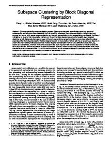
Table 3 shows the results on the ORL dataset. On this dataset, quite a lot of approaches achieve promising performance. Our method still outperforms all the alternative methods significantly. Table 4 shows the results on the video face dataset Notting-Hill. Video face clustering in this dataset is a more challenging task because the appearances of faces often vary significantly due to the lighting conditions, especially light angles which often change drastically. Our method outperforms the closest performing baseline, which is NaMSC with a clear large margin. The performance improvements over NaMSC on four datasets are 5.6%, 4.1%, 1.4%, 6.9% in terms of NMI, respectively. To further demonstrate the significance of the performance improvement, we have done the Student’s ttest of our results. In the experiment, the output on the four datasets of t-test are all 1, which means our method being better than those of other methods is correct with the probability of 1-α = 0.9999. We also note that, directly concatenating all the features is not a proper way since it always performs worse than that of the best single view. On the other hand, although clustering with the best single view achieves promising performance sometimes, it is difficult to choose proper view adaptively. The clustering examples of DiMSC and NaMSC are shown in Figure 3. Limited to the space, we only show a part of (top five best) clusters on the Yale dataset and all the clusters on the Notting-Hill. Accordingly, it is not appropriate to calculate the quantitative result and compare it to the result in Table 1. From Figure 3, it is observed that the results of DiMSC are more promising than those of the second best performer, NaMSC. For example, in the first row in Figure 3(a) corresponding to the same individual, about half of faces are wrongly clustered by NaMSC, while the
(a) Results on Yale (image face dataset)
(b) Results on Notting-Hill (video face dataset)
Figure 3. Some visual clustering results of NaMSC (in the left blue rectangles) and the proposed DiMSC (in the right green rectangles). Each row denotes a face cluster output. The false clustering faces are highlighted by the red rectangles and the incorrect rate in each row is approximately equal to its proportion in the clusters. 0.7 0.6
NMI
0.5 0.4 0.3 0.2
λS=0 λS=0.01
0.1 0
λS=0.02 λS=0.03 0
20
40
60
80
λV
100
120
140
160
180
gence on Extended YaleB as an example in Figure 4 and Figure 5, respectively. As shown in Figure 4, the performance is relatively low while fixing λS = 0, which demonstrates the importance of the smoothness term. The promising performance can be expected when the parameter λS is choose in a range (e.g., [0.01,0.03]). The parameter of diversity term is relatively robust since the performance is stable while λV is chosen in a wide range. The example result in Figure 5 demonstrates that DiMSC converges within a small number of iterations, which empirically proves the proposition 3.1.
Figure 4. Parameter tuning on Extended YaleB.
5. Conclusions
Objective Value
1960 1950 1940 1930
1920 1910 1900 1
2
3
4
5
6
7
Iteration Number
8
9
10
Figure 5. Convergence results Extended YaleB.
proposed DiMSC obtains a much more accurate clustering. We show the parameter tuning and algorithm conver-
In this paper, we considered the subspace clustering under the multi-view setting to utilize the abundant representation of data. We proposed the Diversity-induced Multiview Subspace Clustering approach, which employed the Hilbert-Schmidt Independence Criterion to explicitly enforce the learned subspace representations to be novel with each other. We have shown that the enhanced complementary information could serve as a more helpful complement to multi-view subspace clustering. Our empirical study suggests the proposed approach can effectively explore the underlying complementary information of the given data and outperform all the other multi-view clustering methods used in the experiments.
Acknowledgment This work was supported by National Natural Science Foundation of China (No.61422213,61332012), National Basic Research Program of China (2013CB329305), National High-tech R&D Program of China (2014BAK11B03), and 100 Talents Programme of the Chinese Academy of Sciences.
References [1] M.-R. Amini and C. Goutte. A co-classification approach to learning from multilingual corpora. Machine learning, 79(1):105–121, 2010. [2] R. H. Bartels and G. W. Stewart. Solution of the matrix equation AX + XB = C. Communications of the ACM, 15(9):820–826, 1972. [3] M. B. Blaschko and C. H. Lampert. Correlational spectral clustering. In CVPR, pages 1–8, 2008. [4] A. Blum and T. Mitchell. Combining labeled and unlabeled data with co-training. In COLT, pages 92–100. ACM, 1998. [5] K. Chaudhuri, S. M. Kakade, K. Livescu, and K. Sridharan. Multi-view clustering via canonical correlation analysis. In ICML, pages 129–136, 2009. [6] N. Chen, J. Zhu, and E. Xing. Predictive subspace learning for multi-view data: A large margin approach. In NIPS, pages 361–369, 2010. [7] B. Cheng, G. Liu, J. Wang, Z. Huang, and S. Yan. Multi-task low-rank affinity pursuit for image segmentation. In ICCV, pages 2439–2446, 2011. [8] C. Cortes, M. Mohri, and A. Rostamizadeh. Learning nonlinear combination of kernels. In NIPS, 2009. [9] V. R. de Sa. Spectral clustering with two views. In ICML, pages 20–27, 2005. [10] E. Elhamifar and R. Vidal. Sparse subspace clustering: Algorithm, theory, and applications. TPAMI, 35(11):2765–2781, 2013. [11] H. Fu, D. Xu, S. Lin, D. W. K. Wong, and J. Liu. Automatic optic disc detection in oct slices via low-rank reconstruction. TBME, 62(4):1151–1158, 2015. [12] T. G and L. A. Kernel-based weighted multi-view clustering. In ICDM, pages 675–684, 2012. [13] A. Gretton, O. Bousquet, A. Smola, and B. Sch¨olkopf. Measuring statistical dependence with hilbert-schmidt norms. In Algorithmic learning theory, pages 63–77, 2005. [14] Y. Guo. Convex subspace representation learning from multi-view data. In AAAI, pages 387–393, 2013. [15] H. Hu, Z. Lin, J. Feng, and J. Zhou. Smooth representation clustering. In CVPR, pages 3834–3841, 2014. [16] A. Kumar and H. Daum´e III. A co-training approach for multi-view spectral clustering. In ICML, pages 393–400, 2011. [17] A. Kumar, P. Rai, and H. Daum´e III. Co-regularized multiview spectral clustering. In NIPS, pages 1413–1421, 2011. [18] G. Liu, Z. Lin, S. Yan, J. Sun, Y. Yu, and Y. Ma. Robust recovery of subspace structures by low-rank representation. TPAMI, 35(1):171–184, 2013.
[19] A. Y. Ng, M. I. Jordan, and Y. Weiss. On spectral clustering: Analysis and an algorithm. In NIPS, pages 849–856, 2001. [20] D. Niu, J. G. Dy, and M. I. Jordan. Multiple non-redundant spectral clustering views. In ICML, pages 831–838, 2010. [21] D. Niu, J. G. Dy, and M. I. Jordan. Iterative discovery of multiple alternative clustering views. TPAMI, 36(7):1340– 1353, 2014. [22] N. Quadrianto and C. H. Lampert. Learning multi-view neighborhood preserving projections. In ICML, pages 425– 432, 2011. [23] D. X. Shijie Xiao, Wen Li and D. Tao. Accelerating low rank representation via reformulation with factorized data. In CVPR. 2015. [24] W. Tang, Z. Lu, and I. S. Dhillon. Clustering with multiple graphs. In ICDM, pages 1016–1021, 2009. [25] H. Wang, C. Weng, and J. Yuan. Multi-feature spectral clustering with minimax optimization. In CVPR, pages 4106 – 4113, 2014. [26] W. Wang and Z. Zhou. Analyzing co-training style algorithms. In ECML, pages 454–465, 2007. [27] M. White, X. Zhang, D. Schuurmans, and Y.-l. Yu. Convex multi-view subspace learning. In NIPS, pages 1673–1681, 2012. [28] B. Wu, Y. Zhang, B. Hu, and Q. Ji. Constrained clustering and its application to face clustering in videos. In CVPR, pages 3507–3514, 2013. [29] S. Xiao, M. Tan, and D. Xu. Weighted block-sparse low rank representation for face clustering in videos. In ECCV, pages 123–138. 2014. [30] C. Xu, D. Tao, and C. Xu. A survey on multi-view learning. arXiv preprint arXiv:1304.5634, 2013. [31] C. Xu, D. Tao, and C. Xu. Large-margin multi-view information bottleneck. TPAMI, 36(8):1559–1572, 2014. [32] C. Zhou, C. Zhang, X. Li, G. Shi, and X. Cao. Video face clustering via constrained sparse representation. In ICME, pages 1–6, 2014.