IEEE ANTENNAS AND WIRELESS PROPAGATION LETTERS, VOL. 13, 2014
63
Study of ELF Propagation Parameters Based on the Simulated Schumann Resonances Yi Wang, Member, IEEE, Ye Zhou, and Qunsheng Cao
Abstract—The extremely low frequency (ELF) electromagnetic (EM) wave propagation parameters are obtained and studied based on the simulated Schumann resonances (SRs). To obtain the SRs, ELF EM wave propagation and EM environment of the Earth-ionosphere (E-I) system are rigorously simulated using the geodesic finite-difference time-domain (FDTD) method. Prony’s method is introduced to analyze the simulation results for obtaining the SR parameters. After that, analytical methods combined with the obtained SRs are applied to obtain the propagation parameters including the attenuation rate and the phase velocity. Using the above procedure, propagation parameters are obtained and compared to analytical results. Finally, daily variations of the parameters in the equatorial region are simulated and compared to analytical predictions. Index Terms—Extremely low frequency (ELF), Prony’s method, propagation parameters, Schumann resonances.
I. INTRODUCTION
I
N THE Extremely Low Frequency (ELF) band, propagation of electromagnetic (EM) waves is confined to the cavity formed by the ionosphere and the Earth’s crust (the Earth-ionosphere system, E-I). Because structures of both the ionosphere and the crust have a direct influence on ELF propagation properties, researchers have been studying these properties for years to learn environmental variations of the whole (or parts of the) E-I system. Through the years, researchers have put efforts in all aspects of the ELF study. A review of the ELF study history can be found in [1]. Nowadays, analytical theories of ELF propagation in the E-I system are basically established [2], and recent works have been focused on the ELF applications, such as global weather forecast or earthquake predictions [3]. In these studies, environment simulations of the E-I system are commonly required to accurately describe the ELF propagation properties. However, the nonuniform environment of the ionosphere and the Earth’s crust are usually difficult to simulate, especially using classic analytical theories. In recent years, the time-domain numerical methods [3] have been proposed to
Manuscript received October 21, 2013; revised November 25, 2013; accepted December 16, 2013. Date of publication December 20, 2013; date of current version January 23, 2014. This work was supported by the Natural Science Foundation of China under Grant 61172024 and the Jiangsu Planned Projects for Postdoctoral Research Funds, China, under Grant 1201006C. The authors are with the College of Electronic and Information Engineering, Nanjing University of Aeronautics and Astronautics, Nanjing 210016, China (e-mail:
[email protected]). Color versions of one or more of the figures in this letter are available online at http://ieeexplore.ieee.org. Digital Object Identifier 10.1109/LAWP.2013.2295630
solve ELF-related problems, which have a direct advantage of simulating EM environments, thus making the simulation of ELF EM propagation more accurate. In future ELF studies, it is believed that the accurate solution to ELF application problems will require the combination of both analytical and time-domain numerical methods. In traditional time-domain numerical methods, propagation parameters (such as attenuation rate) are obtained from a comparison of the field amplitudes between two points [4]. In other words, we cannot obtain accurate propagation parameters using traditional time-domain numerical methods and a single observer. In this letter, analytical theory [2] and the geodesic finite-difference time-domain (FDTD) method [3], [5] are combined to study ELF propagation parameters, including the attenuation rate and phase velocity. First, we apply the geodesic FDTD method with environmental details of the E-I system to simulate ELF propagation. In the simulations, geodesic information of the Earth’s surface [6], model of the Earth’s crust [7], and the International Reference Ionosphere (IRI) [8] are considered. Next, Prony’s method [9], [10] is used to analyze the simulated time-domain waveforms to obtain the frequencies and quality factors of Schumann resonances (SRs). Finally, analytical theory [2] is applied to these results to obtain the propagation parameters, including the attenuation rate and the phase velocity. Using this procedure, propagation parameters under different environmental conditions can be obtained using only one observer. We have applied this method to obtain propagation parameters and compared the results to analytical ones. II. TO OBTAIN ELF PROPAGATION PARAMETERS A. Analytical Methods To obtain the ELF propagation parameters in the E-I system, classic analytical theory is applied [2]. According to the telegraph equation method, the phase velocity and the attenuation rate can be written as
(1) is the E-I where is the speed of light, is frequency, propagation parameter, is the phase velocity, and is the attenuation rate. According to theory, can be measured using experiments [11], which requires long-distance observations and large energy consumption. Another method is to use analytical method and analytical E-I system models [2]. However, when using this method, obtaining local parameters
1536-1225 © 2013 IEEE. Personal use is permitted, but republication/redistribution requires IEEE permission. See http://www.ieee.org/publications_standards/publications/rights/index.html for more information.
64
IEEE ANTENNAS AND WIRELESS PROPAGATION LETTERS, VOL. 13, 2014
is also difficult because analytical local E-I system models are difficult to establish and global EM environment variations are difficult to apply (in analytical method). It is believed that SRs are global indicators [12], and their variations depend on the propagation parameters on the great circle between the source and the observer [13]. It is also known that the SR frequencies and the quality factors are directly influenced by the propagation parameter . According to analytical approximation, the SRs of the lossy E-I system satisfy Fig. 1. Conductivity distributions of the ionosphere obtained 80 km above the Earth’s surface at different times of the day: (a) 0400 UT on January 1, 2010; (b) 1600 UT on January 1, 2010.
(2) D. Environment Simulations where are the resonance frequencies of the lossless E-I system and is the Earth’s radius [2]. Because the observation of SRs can be easily completed in specific regions [14], we propose to use the SRs to directly study propagation parameters. Using the inverse of the two groups of equations mentioned above, the propagation parameters of the E-I system can be derived using the SR parameters
(3) Using (1) and (3), the attenuation rate and the phase velocity can be obtained and studied. It is noted that the SR frequencies are discrete; therefore, numerical approximations must be used, which might bring calculation errors to the final results. B. Numerical Methods To obtain local SRs, the geodesic FDTD method [3] is applied to simulate ELF propagation in the E-I system. In this method, the E-I system model is constructed by the alternating planes of transverse-magnetic (TM) and transverse-electric (TE) field components, which are composed of triangular cells and hexagonal cells (including 12 pentagonal cells), respectively. The integral form of Maxwell’s equations is introduced to the model to complete the FDTD process. In this letter, the horizontal resolution is about 250 km, and the radial resolution is 5 km. The calculation space extends to a depth of 100 km into the crust and to an altitude of 100 km above sea level (the top of the ionosphere D region) [10], [15]. C. Prony’s Method Theoretically, the time-domain waveforms simulated using the geodesic FDTD method can be used to obtain the resonant frequencies by Fourier transforms. However, because the E-I system is a lossy one, it is sometimes difficult to obtain accurate SR parameters by directly using Fourier transforms (for example, when the resonances are not obvious in frequency domain). In this case, Prony’s method is a good tool to deal with the simulation data [9], [10]. Using Prony’s method, the resonant frequencies and quality factors can be obtained directly.
Simulations of the global environment are the keys for the simulation of ELF propagation parameters. In this letter, we have considered the ionosphere, the Earth’s crust, and the lightnings to simulate the EM environments of the E-I system. To simulate the ionosphere, IRI data are applied [8], which are generated from the worldwide network of ionosondes that can provide empirical ionosphere models with global distributions and daily variations. Fig. 1 illustrates typical global conductivity distributions of the ionosphere generated from IRI. The sampling interval is 30 in both latitude and longitude directions. The observation height is 80 km, and the data are collected on January 1, 2010. Fig. 1(a) is collected at 0400 UT, and Fig. 1(b) at 1600 UT. In this figure, the daily variations and polar anomalies of the ionosphere are clearly presented. When compared to the ionosphere models [16] applied in analytical theories, the advantage of using IRI data is clearly shown as the inhomogeneity, and daily variations of ionospheric conductivity distributions are fully considered. To simulate lightnings, similar treatments used in [15] and [17] are introduced as exciting sources of the SRs. To simulate the surface and the crust of the Earth (underground model), similar settings are applied as used before [15], in which the EM parameters vary with local geologies (in this letter, the geologies of the Earth’s surface are divided into the ocean, the seaside, and the continent) if not specified. III. RESULTS AND DISCUSSION To analyze ELF propagation parameters, at first we obtained these parameters under different time conditions and compared them to analytical results [2]. In Figs. 2 and 3, attenuation rate is obtained at different times of the day at 32 N, 118 E (Nanjing, China). In Figs. 4 and 5, phase velocity is obtained under similar conditions. In these figures, “Simulated” results mean the simulation results obtained at SR frequencies, and “Approx.” results mean the results interpolated using “Simulated” results. Similar notations are also applied in Figs. 6 and 7. Analytical results are also included in the figures, which are obtained using the ionospheric model introduced in [2] and [18]. In Figs. 2–5, a global average underground model (with and ) is applied in both analytical calculations and time-domain simulations to test the correctness of our method. In Figs. 6 and 7, the nonuniform underground model introduced in Section II is applied in the time-domain simulations. Note that in all the
WANG et al.: STUDY OF ELF PROPAGATION PARAMETERS
65
Fig. 2. Average attenuation rate obtained at 0400 UT, 32 N, 118 E (1200 LT, Nanjing, China) on January 1, 2010, using different methods.
Fig. 5. Average phase velocity obtained at 1600 UT, 32 N, 118 E (2400 LT, Nanjing, China) on January 1, 2010, using different methods.
Fig. 3. Average attenuation rate obtained at 1600 UT, 32 N, 118 E (2400 LT, Nanjing, China) on January 1, 2010, using different methods.
Fig. 6. Average attenuation rate variations in the equatorial region in 24 h.
Fig. 4. Average phase velocity obtained at 0400 UT, 32 N, 118 E (1200 LT, Nanjing, China) on January 1, 2010, using different methods.
Fig. 7. Average phase velocity variations in the equatorial region in 24 h.
figures (Figs. 2–7), the obtained values are average ones of all the propagation directions (propagation direction not discussed here). To obtain the simulation data, we have: 1) simulated ELF propagation using the geodesic FDTD method; 2) noted these TD EM waves at specific places; 3) applied Prony’s method to the noted data to obtain the resonant frequencies and quality factors (SR data); 4) applied the method described in the letter to obtain the propagation parameters; 5) drawn the parameters (discrete data) as “Simulated” data; 6) applied the least-squares method to obtain the “Approx.” data (continuous data).
In Fig. 2, the “Simulated/Approx.” daytime attenuation rates agree well with the analytical result. However, in Fig. 3, the differences among these results become obvious, and the “Simulated/Approx.” nighttime attenuation rate is lower than the analytical results. The differences in phase velocities between the simulation and analytical results are obvious under both day/ night conditions. The simulated daytime phase velocity is lower than the analytical result as presented in Fig. 4, and the nighttime one is larger as presented in Fig. 5. Through these simulations, differences between simulation results (the “Simulated” and “Approx.” ones) and analytical results are obvious except for the daytime attenuation rate. We
66
IEEE ANTENNAS AND WIRELESS PROPAGATION LETTERS, VOL. 13, 2014
believe that these differences are mainly caused by the effect caused by the observer–source distance and the simulation of the E-I system environments including the ionospheric conductivity variations, the nonuniform crust of the Earth, geology information, and lightning current locations. Because propagation parameters are also affected by nearby/global EM environments, the simulation of E-I EM environment details results in better description of the real ELF propagation parameters. Note that these simulation results are obtained in a specific region (Nanjing), and the effect of local environments on observed SRs are to be further studied. Next, we have applied the method to study global variations of propagation parameters with the nonuniform crust and surface of the Earth. In Figs. 6 and 7, we have studied the daily propagation parameter variations in the equatorial region. In these figures, the simulated results (shadowed region) present the variation range of propagation parameters in 24 h. To obtain these results, we have applied the method introduced previously in the equatorial region at 00 E, 30 E, 60 E, , 330 E, separately (total of 12 groups of data). At the same time, the simulations were repeated at 0000 UT, 0400 UT, , 2000 UT, separately (total of six groups of data). Finally, we gathered these data (total of groups of data) and obtained the variation range of the propagation parameters. (Reasons for these variations are presented in the previous paragraph.) The daytime and nighttime analytical values were obtained using the reference method as before [2]. From these two figures, we can see that the variation range of propagation parameters (“simulated” results) is smaller than the analytical values, which means that the variation range of daily ELF propagation parameters in the real E-I system is smaller than that expected using analytical theory. In Fig. 7, the lower edge values of the shadowed region (stands for the lowest simulated phase velocity) are larger than the analytical day results, and the upper edge values of the shadowed region (stands for the largest simulated phase velocity) are smaller than the analytical night results. The same phenomena appear for the attenuation rate in Fig. 6 except that the lower edge of the shadowed region and the analytical day results are almost coincidental. As explained earlier, besides method error, EM environment of the Earth is the main reason for the differences between the simulated values and analytical values. Because the nonuniformity of the Earth’s environment at a specific time can be fully considered in the numerical simulation, the method is believed to provide more accurate results and more rigorous solutions for future studies. IV. CONCLUSION In this letter, we have obtained and studied the ELF propagation parameters based on the SRs. The method is based on the combination of the analytical theory, Prony’s method, and the FDTD method. Through simulations, we have proved that this combination is efficient and promising in studying ELF properties because the EM environment of the E-I system can be fully considered. The advantages of the present method are clearly described in this letter. However, our method to obtain propagation
parameters is based on the SRs, which are difficult to measure or to extract above 50 Hz. This means that our method is only valid below 50 Hz, and to obtain propagation parameters outside this range, new methods are to be further studied. ACKNOWLEDGMENT The authors would like to thank both reviewers for their very valuable remarks and suggestions, which helped to improve the letter significantly. REFERENCES [1] R. Barr, D. Jones, and C. Rodger, “ELF and VLF radio waves,” J. Atmos. Solar-Terrestrial Phys., vol. 62, no. 17–18, pp. 1689–1718, Nov. 2000. [2] A. Kulak and J. Mlynarczyk, “ELF propagation parameters for the finite ground conductivity,” IEEE Trans. Antennas Propag., vol. 61, no. 4, pp. 2269–2275, Apr. 2013. [3] J. J. Simpson, “Current and future applications of 3-D global earthionosphere models based on the full-vector Maxwell’s equations FDTD method,” Surveys Geophys., vol. 30, no. 2, pp. 105–130, Mar. 2009. [4] Y. Wang, H. Xia, and Q. Cao, “Analysis of ELF attenuation rate using the geodesic FDTD algorithm,” in Proc. Int. Conf. Microw. Millim. Wave Technol., 2010, pp. 1413–1415. [5] J. J. Simpson, R. Heikes, and A. Taflove, “FDTD modeling of a novel ELF radar for major oil deposits using a three-dimensional geodesic grid of the earth-ionosphere waveguide,” IEEE Trans. Antennas Propag., vol. 54, no. 6, pp. 1734–1741, Jun. 2006. [6] National Geophysical Data Center, Boulder, CO, USA, “GEODAS Grid Translator—Design-a-Grid,” 2011 [Online]. Available: http://www.ngdc.noaa.gov/mgg/gdas/gd_designagrid.html [7] A. Martinez, A. P. Byrnes, K. G. Survey, and C. Avenue, “Modeling dielectric-constant values of geologic materials: An aid to ground-penetrating radar data collection and interpretation,” Current Res. Earth Sci., vol. Bull. 2, pt. 1, 2001. [8] D. Bilitza and B. Reinisch, “International reference ionosphere 2007: Improvements and new parameters,” Adv. Space Res., vol. 42, no. 4, pp. 599–609, Aug. 2008. [9] J. F. Hauer, C. J. Demeure, and L. L. Scharf, “Initial results in prony analysis of power system response signals,” IEEE Trans. Power Syst., vol. 5, no. 1, pp. 80–89, Feb. 1990. [10] J. J. Simpson, “Global FDTD Maxwell’s equations modeling of electromagnetic propagation from currents in the lithosphere,” IEEE Trans. Antennas Propag., vol. 56, no. 1, pp. 199–203, Jan. 2008. [11] D. White and D. Willim, “Propagation measurements in the extremely low frequency (ELF) band,” IEEE Trans. Commun., vol. COM-22, no. 4, pp. 457–467, Apr. 1974. [12] D. L. Paul and C. J. Railton, “Spherical ADI FDTD method with application to propagation in the earth ionosphere cavity,” IEEE Trans. Antennas Propag., vol. 60, no. 1, pp. 310–317, Jan. 2012. [13] A. Kuak, J. Mynarczyk, S. Ziba, S. Micek, and Z. Nieckarz, “Studies of ELF propagation in the spherical shell cavity using a field decomposition method based on asymmetry of Schumann resonance curves,” J. Geophys. Res., vol. 111, no. A10304, Oct. 2006. [14] K. Schlegel and M. Füllekrug, “50 years of schumann resonance,” Phys. Unserer Zeit, vol. 33, no. 6, pp. 256–26, 2002, Translation: C. Geoghan, 2007. [15] Y. Wang and Q. Cao, “Analysis of seismic electromagnetic phenomena using the FDTD method,” IEEE Trans. Antennas Propag., vol. 59, no. 11, pp. 4171–4180, Nov. 2011. [16] V. Mushtak, “ELF propagation parameters for uniform models of the Earthionosphere waveguide,” J. Atmos. Solar-Terrestrial Phys., vol. 64, no. 18, pp. 1989–2001, Dec. 2002. [17] H. Yang and V. P. Pasko, “Three-dimensional finite difference time domain modeling of the Earth-ionosphere cavity resonances,” Geophys. Res. Lett., vol. 32, no. 3, pp. 4–7, 2005. [18] P. S. Greifinger, V. C. Mushtak, and E. R. Williams, “On modeling the lower characteristic ELF altitude from aeronomical data,” Radio Sci., vol. 42, no. 2, pp. 1–12, Apr. 2007.