2016 IEEE Radar Conference (RadarConf)
Study of Inversion EM Models for Wind Speed Retrieval From Sentinel-1 Data Tran Vu La1, Ali Khenchaf1, Fabrice Comblet1, Carole Nahum2 1
Lab-STICC UMR CNRS 6285, ENSTA Bretagne, 29806 Brest, Cedex 09, France (Email: {tran_vu.la, Ali.Khenchaf, Fabrice.Comblet}@ensta-bretagne.fr) 2 French General Directorate for Armament (DGA), CS 21623, 75509 Paris Cedex 15, France (Email:
[email protected])
Abstract—Sea surface wind speed plays a key parameter in the studies of many oceanic applications, i.e. meteorological forecasting, oil slick observation, ship detection, and wind turbine installation recently. It can be obtained from many available wind sources, i.e. measured data, numeric weather models, etc. However, one of the most well-known ways is the retrieval of wind speed from Synthetic Aperture Radar (SAR) data. For this approach, the studies are based on two principal ways: one uses empirical models and the other is based on electromagnetic calculations. In both indicated approaches, the Geophysical Model Functions (GMFs) are used to describe the dependency of radar scattering from sea surface on surface wind speed and the geometry of observations. By knowing radar scattering and geometric parameters from SAR data, it is possible to invert the GMFs to retrieve wind speed. Then, estimated wind speed by two studied models is compared and evaluated with measured data. Based on the comparisons, the advantages and limits of the studied models are analyzed and discussed. Index Terms—CMOD.5, Geophysical Model Function (GMF), normalized radar cross section (NRCS), sea wind speed retrieval, Sentinel-1 data, Small Perturbation Model (SPM).
I.
INTRODUCTION
Sea surface wind plays an important role for the studies of the other parameters such as wave, current, marine meteorology, and the coupling of oceanic and atmospheric systems. As well, in many oceanic applications, i.e. sea mapping, meteorological forecasting, oil slick observation, ship detection, sea wind speed is a key parameter to obtain good results [1–2]. It can be obtained from many available wind sources, i.e. in situ measurements, numeric weather models, etc. However, the retrieval of wind speed from Synthetic Aperture Radar (SAR) data is particularly preferred due to many interests of SAR satellites: stable operations in most meteorological conditions, revisit mode, high resolution, etc. In fact, wind speed retrieval was carried out from the data of various SAR systems, i.e. L–band JERS-1 [3], C–band Envisat [4], X–band TerraSAR-X [5]. The common point of these studies is the use of empirical (EP) models to estimate wind speed. In such models, the dependency of radar backscattering from sea surface on wind speed and the geometry of observations, i.e. wind direction relative to radar look, incident angle, is described by the Geophysical Model Functions (GMFs). Such GMFs have been constructed and This work is supported by the French General Directorate for Armament (Direction Générale de l'Armement) in the frame of the SIMUSO project.
978-1-5090-0863-6/16/$31.00 ©2016 IEEE
validated by the series of satellite scatterometer missions. In C–band, one can find the GMFs as CMOD.4 [6], CMOD.IFR2 [7], CMOD.5 [8], and CMOD.5N [9]. By knowing radar scattering and the parameters of geometric observations, it is possible to invert the GMFs to retrieve wind speed. In contrast to the EP models, the GMFs in the electromagnetic (EM) models have been constructed and validated by the physical principals of reflection and diffraction between radar signal and sea surface. Obviously, it is much more difficult to invert the GMFs of EM models to retrieve wind speed, since they concern many parameters and conditions. Therefore, our priority in this paper is the selection of a simple EM model for the inversion purpose. Depending on different approaches, one can find the EM models based on exact methods, i.e. Method of Moment (MoM) [10], Forward– Backward Method (FBM) [11], or asymptotic methods, i.e. Two-Scale Model (TSM) [12], Small Slope Approximation (SSA) [13], and Small Perturbation Method (SPM) [12]. The advantages and limits of these models have been analyzed and discussed in [13]. The TSM, SSA, MoM, and FBM models can describe radar scattering from sea surface including different scales of sea waves (long-, intermediate-, and short-scale waves). The GMFs in such models are generally complicated due to a lot of variables and relations. Meanwhile, the description of the GMF in the SPM model (hereafter called SPM) is quite simpler and clearer, since it concerns principally short-scale waves. Under the point of view of inversion problem, SPM seems to be more appropriate than the others due to its simple description, and then it can offer wind speed estimates more rapidly. This is also the objective of our study. The rest of the paper is organized as follows. In Section II, radar backscattering from sea surface calculated by SPM and CMOD.5 in respect to wind speed will be compared and evaluated. In Section III, estimated wind speed by the two studied models from a Sentinel-1 image in VV polarization (VV-pol) is compared and evaluated with ground-truth data from the meteorological observation stations. In Section IV, the conclusions and perspectives of this study are discussed. II.
METHODOLOGY
A. Small Perturbation Model (SPM) 1) Description of GMF of SPM
For the monostatic case of radar scattering, the relation between sea surface roughness and radar backscattering expressed by SPM is shown as [12]
2
𝑠 𝜎𝑝𝑝 = 8|𝑘 2 𝜎 𝑐𝑜𝑠² 𝜃 𝛼𝑝𝑝 | 𝑊(𝑘𝑥 + 𝑘𝑠𝑖𝑛𝜃, 𝑘𝑦 )
where σpp represents the normalized radar cross section (NRCS) in VV-pol or HH-pol, k is the radar wave number and kx, ky are the x-axis and y-axis components of k, respectively. The angle θ indicates the incident one and also the backscattering one in monostatic case. The Bragg coefficient αpp is described as a function of seawater permittivity εr and θ. The parameters σ and W represent the standard deviation and normalized roughness spectrum of sea surface waves, respectively. As described in [12], the Bragg coefficients in VV- and HH-pol, αVV and αHH, are calculated as 𝛼𝑉𝑉 =
(𝜀𝑟 − 1)[𝜀𝑟 (1 + sin² 𝜃) − sin² 𝜃] [𝜀𝑟 cos 𝜃 + √(𝜀𝑟 − sin ²𝜃)]
𝛼𝐻𝐻 =
2
𝜀𝑟 − 1 2
[cos 𝜃 + √(𝜀𝑟 − 𝑠𝑖𝑛²𝜃)]
(a)
(2),
(3),
The seawater permittivity εr is dependent on temperature T and salinity S. According to our study (will be shown in the conference), T and S do not have any significant effects on the calculations of radar backscattering. 2) Surface Wave Roughness Spectrum In contrast to T and S, sea surface roughness spectrum is a crucial parameter for NRCS calculations. It concerns a lot of variables, in particular wind direction and wind speed, which are the two favorite parameters in this paper. For the simple description reason, σ and W in (1) are replaced by directional surface wave spectrum 𝑆(𝐾, 𝛷), with wave propagation referenced to wind direction 𝛷. The spectrum 𝑆(𝐾, 𝛷) is generally described by two parts as
𝑆(𝐾, 𝛷) = 𝑆(𝐾, 0) × 𝑓(𝐾, 𝛷)
where 𝑆(𝐾, 0) is the omnidirectional spectrum and 𝑓(𝐾, 𝛷) is the angular spreading function. The omnidirectional spectrum 𝑆(𝐾, 0) concerns wind speed, while both wind speed and wind direction effects are present in 𝑓(𝐾, 𝛷). By determining 𝑆(𝐾, 𝛷) and 𝛷, wind speed can be estimated. One should note that 𝐾 in (2) is the wavenumber of ocean waves. For SPM (or Bragg resonance), 𝐾 relates to the radar wavenumber k as 𝐾 = 2k × sinθ, where θ is the radar incident angle. The models of sea surface roughness spectrum can be divided into two categories: semi-empirical and empirical models. The semi-empirical approach can be found in the studies of Elfouhaily et al. [14], Romeiser et al. [15], Donelan et al. [16], and Kudryavtsev et al. [17]. In such models, wave spectrum is determined from energy balance equation. It is assumed to include two parts: wind wave spectrum and
(b) Fig. 1. Comparison of NRCS calculated by SPM-Elf, SPM-Hwa08 and CMOD.5 in VV-pol for θ = 30° and θ = 45°. (a) Up-wind direction ( 𝛷 = 0°). (b) Cross-wind direction ( 𝛷 = 90°).
spectrum of parasitic capillaries. Meanwhile, in the empirical approach proposed by Hwang [18–19], the surface waves are principally produced by wind input. In order to evaluate the impact of different wave models on wind speed estimation, we study in this paper SPM with the Elfouhaily model [14] and with the Hwang 2008 model [18]. B. CMOD.5 A general form of the GMFs described in the EP models is defined as [6–9] 0 𝜎𝑉𝑉 = 𝐴[1 + 𝑏1 × cos 𝛷 + 𝑏2 × cos 2𝛷]𝐵
(3),
where A, B, b1, b2 are the functions of wind speed at the height 0 of 10 m (U10) and incident angle θ. By determining 𝜎𝑉𝑉 and θ from SAR data and knowing 𝛷, U10 can be estimated by inverting (3). As presented, the C–band GMFs (CMOD.4, CMOD.IFR2, CMOD.5, and CMOD.5N) have been developed corresponding to different in situ measurements. The last two ones seem to give better wind speed estimates than the first two ones, especially for the estimation of high wind speed. Therefore, we select CMOD.5 for wind speed retrieval from
Sentinel-1 data in this paper. Since CMOD.5 is only defined for VV-pol, a polarization ratio, PR, should be used for the SAR data in HH-pol [20–21]. C. Comparison between SPM and CMOD.5 Fig. 1 shows the VV-pol NRCS calculated by SPM and CMOD.5 for up-wind direction (𝛷 = 0°) and cross-wind direction (𝛷 = 90°). The NRCS calculated in HH-pol will be presented during the conference. As indicated, two models of wave roughness spectrum are studied with SPM: Elfouhaily (hereafter called SPM-Elf), and Hwang 2008 (hereafter called SPM-Hwa08). Two values of incident angles are considered: θ = 30° and θ = 45°. They correspond to the validity domain of SPM. As well, the studied wind speed is limited at U10 = 13 m/s, since SPM only works well under the conditions of slightly rough sea surface. At θ = 30°, both NRCS curves expressed by SPM are lower than that of the CMOD.5. This is noted for both up-wind and cross-wind directions. However, the NRCS level calculated by SPM-Hwa08 is much closer to the result offered by CMOD.5 (2 dB difference), especially for low wind speed (below 9 m/s). Meanwhile, for this wind regime the difference of NRCS calculated by SPM-Elf and CMOD.5 is significant (more 4 dB). At θ = 45°, for up-wind direction SPM-Elf and CMOD.5 give quite similar NRCS level with regard to wind speed, while the level calculated by SPM-Hwa08 is overestimated (about 4 dB). For cross-wind direction, both NRCS curves calculated by SPM are higher than the one expressed by CMOD.5 (about 2–4 dB). Based on the compared results in Fig. 1, one can note that SPM cannot calculate well radar backscattering from sea surface for low incident angles, regardless of wave roughness spectrum models. Therefore, estimated wind speed by SPM is probably not accurate. Meanwhile, the estimation of wind speed performed by SPM is improved for moderate incident angles, notably above 40°. The SPM with the Hwang wave model offers better wind speed estimates for lower moderate incident angles than upper ones. Meanwhile, estimated wind speed by SPM with the Elfouhaily wave model is closer to the one by CMOD.5 for upper moderate wind speed. III.
WIND FIELD RETRIEVAL
The Sentinel-1 image of Iroise Coast (France) used in this paper was acquired on Jan 16, 2015 from 18:04:24 UTC to 18:04:59 UTC, with Interferometric Wide Swath (IWS) mode. It is the data type of ground-range, multi-look, and high resolution (GRD-HR), which allows reducing speckle noise. However, it also reduces the spatial resolution of acquired images. The polarization of this image is VV-pol, and the radar incident angle to acquire it is from 30° to 45°. The Sentinel-1 Toolbox [22] is used to extract NRCS, θ, and the information of the image geographical location (latitude and longitude) from the acquired images. The estimated wind speed by SPM and CMOD.5 is shown in Fig. 2. The color bar has the same scale (0–12 m/s) in three cases. As expected in Fig. 1, for θ = 30°–35° SPM-Hwa08 and CMOD.5 give quite similar wind speed estimates, while SPMElf overestimates wind speed about 2–4 m/s. On the contrary,
for θ = 40°–45° estimated wind speed by SPM-Elf and CMOD.5 is very close, while the one given by SPM-Hwa08 is underestimated about 2-3 m/s. The difference in the estimation of wind speed performed by SPM with two wave spectrum models shows that both studied approaches (semi-empirical and empirical) are not the optimal solutions. A compromise of wind speed estimation (i.e. 2-3 m/s difference) should be accepted in this case. Compared to the measured data from the meteorological observation stations [24], the estimated wind speed by CMOD.5 is quite similar (except the first point). For SPM-Hwa 08, estimated wind speed is close to measured data for θ below 40°, while estimated results by SPM-Elf are generally higher than measured data (about 2–3 m/s). The wind directions in Fig. 2a have been extracted by the Local Gradient (LG) method [23]. They are used in SPM as described in (1) and in CMOD.5 as shown in (2) to estimate wind speed. The resolution cell of extracted wind directions in this case is 5 km × 5 km. They are very close to the measured data (red arrows) from the meteorological observation stations. This shows that the selected wind cell is reasonable to obtain accurate wind directions. The deviations between extracted and measured wind directions in Fig. 2a are about 15–20°. These errors are tolerable since they do not affect significantly the estimation of wind speed performed by both SPM and CMOD.5. Indeed, as shown in Fig. 3, for 45° error in the retrieval of wind direction, maximal difference in the estimation of wind speed is only 2–3 m/s. IV.
CONCLUSION AND PERSPECTIVES
This paper presents the retrieval of wind speed from Sentinel-1 data using the EM and EP models. For the EM models, SPM has been selected due to its simple description. This is more appropriate for the inversion problem. Wave roughness spectrum is a crucial parameter for SPM to calculate NRCS, and then for the retrieval of wind speed. Two wave spectrum models have been studied in this paper: the semiempirical model described by Elfouhaily, and the empirical model proposed by Hwang in 2008. For the EP models, CMOD.5 has been chosen, since it can give good wind speed estimation in most cases of wind regimes. For low incident angles, SPM does not estimate well wind speed, regardless of wave roughness spectrum models. For lower moderate angles, SPM with the Hwang 08 model offers better wind speed estimates than SPM with the Elfouhaily model. On the contrary, for upper moderate incident angles, estimated wind speed by SPM with the Elfouhaily model is closer to the one offered by CMOD.5. In next steps, the other EM models as TSM or SSA should be used to improve the estimation of wind speed from SAR data, especially for high wind speed (> 13 m/s) and for lower radar incident angles, notably below 30°. This is particularly necessary, since such EM models can describe sea surface with different ocean wave scales. In addition, the inhomogeneous description of surface wave spectrum, instead of standard models used in this paper, will be studied to better assess their impact on the estimation of wind speed.
ACKNOWLEDGMENT The Sentine-1 SAR images and Sentinel-1 Toolbox are provided by the European Space Agency (ESA) via https://scihub.esa.int/. The in situ measurements are given by Météo France via http://www.infoclimat.fr/. REFERENCES [1]
M.Y. Ayari, A. Coatanhay, A. Khenchaf, “The influence of ripple damping on electromagnetic bistatic scattering by sea surface,” IEEE IGARSS’05, pp. 1345–1348, Seoul, Korea, July 2005. [2] M. R. Pino, L. Landesa, J. L. Rodriguez, F. Obelleiro, and R. J. Burkholder, “The Generalized Forward–Backward Method for Analyzing the Scattering from Targets on Ocean-Like Rough Surfaces,” IEEE Trans. on Ant. & Prop., Vol. 47, No. 6, pp. 961–969, Jun. 1999. [3] T. Shimada, H. Kawamura, and M. Shimada, “An L-Band Geophysical Model Function for SAR Wind Retrieval Using JERS-1 SAR,” IEEE Trans. on Geo. & Rem. Sens., Vol. 41, No. 3, pp. 518–531, Mar. 2003. [4] G. K. Carvajal, L. Eriksson, and L. Ulander, “Retrieval and Quality Assessment of Wind Velocity Vectors on the Ocean With C-Band SAR,” IEEE Trans. on Geo. & Rem. Sens., Vol. 52, No. 5, pp. 2519– 2537, May 2014. [5] X-M. Li and S. Lehner, “Algorithm for Sea Surface Wind Retrieval From TerraSAR-X and TanDEM-X Data,” IEEE Trans. on Geo. & Rem. Sens., Vol. 52, No. 5, pp. 2928–2939, May 2014. [6] Ad Stoffelen and David Anderson, “Scatterometer data interpretation: Estimation and validation of the transfer function CMOD4,” J. Geophys. Res., Vol. 102, No. C3, pp. 5767–5780, Mar. 1997. [7] Y. Quilfen, B. Chapron, T. Elfouhaily, K. Katsaros, and J. Tournadre, “Observation Of tropical cyclones by high-resolutions scatterometry,” J. Geophys. Res., Vol. 103, No. C4, pp. 7767–7786, Apr. 1998. [8] H. Hersbach, A. Stoffelen, and S. de Haan, “An improved C-band scatterometer ocean geophysical model function: CMOD5,” J. Geophys. Res., Vol. 112, No. C3, pp. C03006, Mar. 2007. [9] J. Verspeek, A. Stoffelen, M. Portabella, H. Bonekamp, C. Anderson, and J. F. Saldaña, “Validation and Calibration of ASCAT Using CMOD5.n,” IEEE Trans. on Geo. & Rem. Sens., Vol. 48, No. 1, pp. 386–395, Jan. 2010. [10] Andreas Colliander, and Pasi Ylä-Oijala, “Electromagnetic Scattering From Rough Surface Using Single Integral Equation and Adaptive Integral Method,” IEEE Trans. on Ant. & Prop., Vol. 55, No. 12, pp. 3639–3646, Dec. 2007. [11] D. Holliday, L. L. DeRaad, and G. J. St-Cyr, “Forward-Backward: A new method for computing low-grazing angle scattering,” IEEE Trans. on Ant. & Prop., Vol. 44, No. 5, pp. 722–729, May 1996.
[12] A. Khenchaf, ‘‘Bistatic scattering and depolarization by randomly rough surface: Application to natural rough surface in X-band,’’ Wave in Random and Complex Media, Vol. 11, No. 2, pp. 61–89, 2001. [13] A. Awada, Y. Ayari, A. Khenchaf, and A. Coatanhay, “Bistatic scattering from an anisotropic sea surface: Numerical comparison between the first-order SSA and the TSM models,” Wave in Random and Complex Media, Vol. 16, No. 3, pp. 383–394, Feb. 2007. [14] T. Elfouhaily, B. Chapron and K. Katsaros, “A Unified Directional Spectrum for Long and Short Wind-Driven Waves,” J. of Geophys. Res., Vol. 102, No. C7, pp. 15781–15796, 1997. [15] R. Romeiser, W. Alpers, and V. Wismann, “An improved composite surface model for the radar scattering cross section of the ocean surface: 1. Theory of the model and optimization/validation by scatterometer data,” J. Geophys. Res., Vol. 102, No. C11, pp. 25237–25250, Nov. 1997. [16] M. A. Donelan, J. Hamilton, and W. H. Hui, “Directional spectra of wind‐generated waves”, Philos. Trans. R. Soc. London, Vol. 315, No. 1534, pp. 509–562, 1985. [17] V. Kudryavtsev, D. Hauser, G. Caudal, and B. Chapron, “A semiempirical model of the normalized radar cross-section of the sea surface: 1. Background model”, J. Geophys. Res., Vol. 108(C3), 8054, doi:10.1029/2001JC001003, 2003. [18] Paul A. Hwang, “Observations of swell influence on ocean surface roughness,” J. Geophys. Res., Vol. 113, C12024, doi:10.1029/2008JC005075, 2008. [19] Paul A. Hwang, “A Note on the Ocean Surface Roughness Spectrum,” J. of Atm. & Oce. Tech., Vol. 28, pp. 436–443, 2010. [20] J. Horstmann, W. Koch, S. Lehner, and R. Tonboe, “Ocean winds from RADARSAT-1 ScanSAR,” Can. J. Remote Sens., Vol. 28, No. 3, pp. 524–533, Jun. 2002. [21] G. Liu, X. Yang, X. Li, B. Zhang, W. Pichel, Z. Li, and X. Zhou, “A Systematic Comparison of the Effect of Polarization Ratio Models on Sea Surface Wind Retrieval From C-Band Synthetic Aperture Radar,” IEEE J. of Selected Topics in Applied Earth Obs. & Rem. Sens., Vol. 6, No. 3, pp. 1100–1108, Jun. 2013. [22] Sentinel-1 Toolbox 64 bits. Available online: https://sentinel.esa.int/web/sentinel/toolboxes/sentinel-1. [23] Wolfgang Koch, “Directional Analysis of SAR Images Aiming at Wind Direction,” IEEE Trans. on Geo. & Rem. Sens., Vol. 42, No. 4, pp. 702– 710, Apr. 2004. [24] Available online: http://www.infoclimat.fr.
N
N 11.5 8.1 7.7 7.6 8.0
5.4
3.0
40° 30°
45°
40°
35°
30°
45°
35°
(a)
(b)
N
40° 30°
45°
35°
(c) Fig. 2. Estimated wind speed from the Sentinel-1 image of Iroise Coast (France), acquired in IWS mode on Jan 16, 2015 from 18:04:24 UTC to 18:04:59 UTC. The estimation of wind speed is performed by (a) CMOD.5, (b) SPM-Hwa08, and (c) SPM-Elf.
Fig. 3. Comparison of NRCS calculated by SPM and CMOD.5 in respect to wind speed for different wind directions (up-wind, 45°, cross-wind). The incident angle in this case is θ = 40°.