also in the case of text classification, but naive Bayes can obtain near optimal ... a melody has been generated by a class cj is the multinomial distribution,.
Style recognition through statistical event models Carlos P´erez-Sancho∗ Jos´e M. I˜ nesta Jorge Calera-Rubio {cperez,inesta,calera}@dlsi.ua.es Grupo de Reconocimiento de Formas e Inteligencia Artificial Departamento de Lenguajes y Sistemas Inform´ aticos Universidad de Alicante, E-03080 Alicante, Spain
Abstract The automatic classification of music fragments into styles is one challenging problem within the music information retrieval (MIR) domain and also for the understanding of music style perception. This has a number of applications, including the indexation and exploration of musical databases. Some technologies employed in text classification can be applied to this problem. The key point here is to establish the music equivalent to the words in texts. A number of works use the combination of intervals and duration ratios for this purpose. In this paper, different statistical text recognition algorithms are applied to style recognition using this kind of melody representation, exploring their performance for different word sizes.
1
Introduction
The automatic machine learning and pattern recognition techniques, successfully employed in other fields, can be also applied to music analysis. One of the tasks that can be posed is the modelization of the music style. Immediate applications are the classification, indexation, and content-based search in digital music libraries, where digitised (MP3), sequenced (MIDI) or structurally represented (XML) music can be found. For example, the computer could be trained in the user musical taste in order to look for that kind of music over large musical databases. A number of recent papers explore the capabilities of machine learning methods to recognise music style, either using audio or symbolic sources. Among the first, for example, ? use self-organising maps (SOM) to pose the problem of organising music digital libraries according to sound features of musical themes, ∗ Corresponding
author. Telephone: +34965903772. Fax: +34965909326.
1
in such a way that similar themes are clustered, performing a content-based classification of the sounds. ? present a system based on neural networks and support vector machines able to classify an audio fragment into a given list of sources or artists. Also ? describe a neural system to recognise music types from sound inputs. Dealing with symbolic data, we can find a recent work by ?, where the authors show the ability of grammatical inference methods for modeling musical style. A stochastic grammar for each musical style is inferred from examples, and those grammars are used to parse and classify new melodies. In (?) the authors compare the performance of different pattern recognition paradigms to recognise music style using descriptive statistics of pitches, intervals, durations, silences, etc. Other approaches like hidden Markov models (?) or different classifiers (?) have been used to pose this problem. Our aim is to explore the capabilities of text categorization algorithms to solve problems relevant to computer music. In this paper, some of those methods are applied to the recognition of musical genres from a symbolic representation of melodies. Some styles like jazz, classical, ragtime or gregorian have been chosen as an initial benchmark for the proposed methodology due to the general agreement in the musicology community about their definition and limits.
2 2.1
Methodology Data sets
Experiments were performed using two different corpora. Both of them are made up of MIDI files, containing monophonic sequences. The first corpus is a set of MIDI files from Jazz and Classical music collected from different web sources, without any processing before entering the system. The melodies are real-time sequenced by musicians, without quantization. The corpus is made up of 110 MIDI files, 45 of them being classical music and 65 being jazz music. The length of the corpus is around 10,000 bars (40,000 beats). Classical melody samples were taken from works by Mozart, Bach, Schubert, Chopin, Grieg, Vivaldi, Schumann, Brahms, Beethoven, Dvorak, Haendel, Paganini and Mendelssohn. Jazz music samples were standard tunes from a variety of well known jazz authors including Charlie Parker, Duke Ellington, Bill Evans, Miles Davis, etc. The second corpus is that used by Cruz et al. (?). It consists of 300 MIDI files, from three different styles: Gregorian, passages from the sacred music of J. S. Bach (Baroque), and Scott Joplin ragtimes; with 100 files per class. In this corpus, the melodies were step-by-step sequenced, and are much shorter (around 10 bars per file in average) than in the former set.
2
2.2
Encoding
Since we are trying to use text categorization approaches, there is a need to find an appropriate encoding, something like music words, that captures relevant information of the data and is suitable for that kind of algorithms to be applied. The encoding used in this work has been inspired in the encoding method proposed in (?). This method makes use of pitch intervals and inter onset time ratios (IOR) to build series of symbols of a given length. The encoding of MIDI files is performed as follows: Melody extraction. The melody track from each MIDI file is analyzed, obtaining the pitch and duration for each note. Durations are calculated as the number of ticks between the onset of the note and that of the next, ingnoring all intermediate rests. As a result, a pair of values {pitch,duration} is obtained for each note in the analyzed track. n-word extraction. Next, the melody is divided into n-note windows. For each window, a sequence of intervals and duration ratios is obtained (see Figure ?? for an example), calculated using Equations (??) and (??) respectively. Ii = P itchi+1 − P itchi Onseti+2 − Onseti+1 Ri = Onseti+1 − Onseti
(i = 1, . . . , n − 1)
(1)
(i = 1, . . . , n − 2)
(2)
Each n-word is defined then as a sequence of symbols: [I1 R1 . . . In−2 Rn−2 In−1 Rn−1 ]
(3)
[Figure 1 about here.] n-words coding. The n-words obtained in the previous step are mapped into sequences of alphanumeric characters (see Figure ??), that will be named nwords due to the equivalence we want to establish between melody and text. As the number of ASCII printable characters is lower than all possible intervals, a non-linear mapping through a hyperbolic tangent is used to assign characters to different interval values. For the IOR the mapping is also performed and has the additional advantage of performing an adaptative quantization of the original MIDI depending on the length of the pair of notes involved. Both mappings have also the property of imposing limits to the permitted ranges for both intervals and IOR. The encoding alphabet consists of 53 symbols for intervals and 21 for IOR. In order to illustrate the distribution of codes for both styles, histograms of intervals and IOR are displayed in Figure ??. Note the different frequencies for each style, that are in the basis of the recognition system. [Figure 2 about here.]
3
Stop words. A melody can contain pairs of notes separated by long rests, that can last for some seconds, or even minutes. Consecutive notes separated by this kind of rests are not really related, so the next note can be considered as the beginning of a new melody. Therefore, it is not fair encoding together consecutive notes separated by a large rest in a melody. Considering this, a silence threshold is established, in a way that when a rest longer than this threshold is found, no words are generated across it. This restriction implies that, for each rest longer than this threshold, n − 1 words less are encoded. This threshold has been empirically set to a rest of four beats.
2.3
Word lengths
In order to test the classification ability of different word lengths, n, a range for n ∈ {2, 3, 4, 5, 6, 7} has been established. The shorter n-words are less specific and provide more general information and, on the other hand, larger n-words may be more informative but the models based on them will be more difficult to train. Using the encoding scheme, the vocabulary size for each n is |Vn | = (53 × 21)n−1 words. In Table ?? the number of words that have been extracted from the training set for each length is displayed. [Table 1 about here.]
2.4
Naive Bayes Classifier
The naive Bayes classifier, as described in (?), has been used. In this framework, classification is performed following the well-known�Bayes’ classification rule. In a context where we have a set of classes cj ∈ C = c1 , c2 , . . . , c|C| , a melody xi is assigned to the class cj with maximum a posteriori probability, in order to minimize the probability of error: P (cj |xi ) =
P (cj )P (xi |cj ) . P (xi )
(4)
where P (cj ) is the a priori probability of class cj , P (xi |cj ) is the probability of P|C| xi being generated by class cj , and P (xi ) = j=1 P (cj )P (xi |cj ). Our classifier is based on the naive Bayes assumption, i.e. it assumes that all words in a melody are independent of each other, and also independent of the order they are generated. This assumption is clearly false in our problem and also in the case of text classification, but naive Bayes can obtain near optimal classification errors in spite of that (?). To reflect this independence �assumption, melodies can be represented as a vector xi = xi1 , xi2 , . . . , xi|V| , where each component xit ∈ {0, 1} represents whether the word wt appears in the document or not, and |V| is the size of the vocabulary. Thus, the class-conditional probability of a document P (xi |cj ) is given by the probability distribution of words wt in class cj , which can be learned from a labelled training sample, X = {x1 , x2 , . . . , xn }, using a supervised learning method.
4
2.4.1
Multivariate Bernoulli model (MB)
� In this model, melodies are represented by a binary vector xi = xi1 , xi2 , . . . , xi|V| , where each xit ∈ {0, 1} represents whether the word wt appears at least once in the melody. Using this approach, each class follows a multivariate Bernoulli distribution: P (xi |cj ) =
|V| Y
xit P (wt |cj ) + (1 − xit )(1 − P (wt |cj ))
(5)
t=1
where P (wt |cj ) are the class-conditional probabilities of each word in the vocabulary, and these are the parameters to be learned from the training sample. Given a labelled sample of melodies X = {x1 , x2 , . . . , xn }, Bayes-optimal estimates for probabilities P (wt |cj ) can be easily calculated by counting the number of occurrences of each word in the corresponding class: P (wt |cj ) =
1 + Mtj 2 + Mj
(6)
where Mtj is the number of melodies in class cj containing word wt , and Mj is the total number of melodies in class cj . Also, a Laplacean prior has been introduced in the equation above to smooth probabilities. Prior probabilities for classes P (cj ) can be estimated from the training sample using a maximum likelihood estimate: Mj (7) P (cj ) = |X | Classification of new melodies is performed then using Equation ??, which is expanded using Equations ?? and ??. 2.4.2
Multinomial model (MN)
This model takes into account word frequencies in each melody, rather than just the occurrence or non-occurence of words as in the MB model. In consequence, documents are represented by a vector, where each component xit is the number of occurrences of word wt in the melody. In this model, the probability that a melody has been generated by a class cj is the multinomial distribution, assuming that the melody length in words, |xi |, is class-independent (?): P (xi |cj ) = P (|xi |)|xi |!
|V| Y P (wt |cj )xit xit ! t=1
(8)
Now, Bayes-optimal estimates for class-conditional word probabilities are: P (wt |cj ) =
1 + Ntj P|V| |V| + k=1 Nkj
(9)
where Ntj is the sum of occurrences of word wt in melodies in class cj . Class prior probabilities are also calculated as for MB. 5
2.4.3
Multivariate Bernoulli mixture model (MMB)
Both MB and MN have proven to achieve quite good results in text classification (??), but they can be improved assuming that probabilities of words follow a more complex distribution within a class. Imagine that we want to model the distribution of musical words in a sample of classical music melodies, which is formed in equal shares by Baroque and Renaissance scores. It is likely that both subsets have different distributions of words, so that we could find some words very common in Baroque music that don’t usually appear in Renaissance music. In this case, using the MB model, Bayes-optimal estimates for these words in the whole set would be just a half of the real ones in Baroque, and much greater than their real value in Renaissance. Intuitively, it would be more accurate to find the separate estimates for each substyle and then combine them to model the whole style. However, since the only information we have about these sequences is that all of them belong to classical music, finding the optimal estimates for each substyle is not straightforward. Furthermore, this problem becomes more complex when inner class structure (i.e. the number and proportions of the subsets) is not known a priori. To solve this problem, we will use here finite mixtures of multivariate Bernoulli distributions, as they have been successfully applied in text classification tasks (??). A finite mixture model is a probability distribution formed by a number of components M : M X P (xi ) = πm P (xi |pm ) (10) m=1
PM where πm are the mixing proportions, � that must satisfy the restriction m=1 πm = 1; and pm = pm1 , pm2 , . . . , pm|V| are the component prototypes. Since we will model each class as a mixture of multivariate Bernoulli distributions, each component distribution P (xi |pm ) is calculated using Equation ??, substituting P (wt |cj ) with its corresponding value pmt . Now we face the problem of obtaining optimal estimates for parameters Θ = t (π1 , . . . , πM , p1 , . . . , pM ) . This can be achieved using the EM algorithm (??), but to be applicable, EM algorithm requires that the problem be formulated as an incomplete-data problem. To do this, we can think of each sample document xi as an incomplete vector (?), where zi = (zi1 , . . . , ziM ) is the missing data and indicates which component of the mixture the document belongs to (with 1 in the position corresponding to the component and zeros elsewhere). Then, the EM proceeds iteratively to find the parameters that maximize the log-likelihood of the complete data: LC (Θ|X, Z) =
n X M X
zim (log πm + log P (xi |pm )) .
(11)
i=1 m=1
In each iteration, the EM algorithm performs two steps. The E-step computes the expected value of the missing data given the incomplete data and 6
the current parameters. Each zim is replaced by the posterior probability of xi being generated by component m: πm P (xi |pm ) zim = PM k=1 πk P (xi |pk )
(i = 1, . . . , n; m = 1, . . . , M )
(12)
The M-step updates then the maximum likelihood estimates for the parameters: Pn zim πm = i=1 (m = 1, . . . , M ) (13) Pn n zim xi (m = 1, . . . , M ) (14) pm = Pi=1 n i=1 zim Once the optimal parameters have been obtained, classification can be then performed expanding Equation ?? using Equations ?? and ??.
2.5
Feature selection
The methods explained above use a representation of musical pieces as a vector of symbols. A common practice in text classification is to reduce the dimensionality of those vectors by selecting the words which contribute most to discriminate the class of a document. A widely used measure to rank the words is the average mutual information (AMI) (?). For the MB model, the AMI is calculated between (1) the class of a document and (2) the absence or presence of a word in the document. We define C as a random variable over all classes, and Ft as a random variable over the absence or presence of word wt in a melody, Ft taking on values in ft ∈ {0, 1}, where ft = 0 indicates the absence of word wt and ft = 1 indicates the presence of word wt . The AMI is calculated for each wt as1 : I(C; Ft ) =
|C| X
X
P (cj , ft ) log
j=1 ft ∈{0,1}
P (cj , ft ) P (cj )P (ft )
(15)
where P (cj ) is the number of melodies for class cj divided by the total number of melodies; P (ft ) is the number of melodies containing the word wt divided by the total number of melodies; and P (cj , ft ) is the number of melodies in class cj having a value ft for word wt divided by the total number of melodies. In the MN model, the AMI is calculated between (1) the class of the melody from which a word occurrence is drawn and (2) a random variable over all the word occurrences, instead of melodies. In this case, Equation ?? is also used, but P (cj ) is the number of word occurrences appearing in melodies in class cj divided by the total number of word occurrences, P (ft ) is the number of occurrences of the word wt divided by the total number of word occurrences, and P (cj , ft ) is the number of occurrences of word wt in melodies with class label cj , divided by the total number of word occurrences. 1
The convention 0 log 0 = 0 was used, since x log x → 0 as x → 0.
7
3
Results
The style recognition ability of the different word sizes has been tested. For each model, the naive Bayes classifier has been applied to the words extracted from the melodies in our training set. The experiments have been made following a leave-one-out scheme: the training has been constructed with all the melodies but one, kept for test. After training the model, the words in the test melody are extracted and used to classify it. The presented results are the percentage of successfully classified melodies. The evolution of the classification as a function of the significance of the information used is presented in the graphs in Figure ??. For this, the words in the training set have been ordered according to their AMI value. After that, experiments using the best rated words (|V| in the graphs) have been performed. [Figure 3 about here.] Note that the results were not conclusive in terms of the different statistical models, since all the methods performed comparatively. There is a tendency of Bernoullis to classify better for small values of |V| while multinomials seem to provide better results for larger |V|. This points to the fact that, when few words are available it is important the presence or not of them in order to perform the decision (binomial probabilities), but for larger vocabularies it is more important the frequencies of the different words (multinomial). Table ?? shows the best results obtained in the experiments. The best accuracy was obtained for the word size n = 3, reaching a 94.3% of successful style identification. Large n-words only perform well (above 80%) for very small |V| values, and get worse rapidly for larger values. This preference for little specific information points to the fact that the method is indeed able to classify but maybe the training set is small, and the results could be improved for larger models with more training melodies. [Table 2 about here.] Also, the values for precision and recall have been studied. There is a tendency to get low percentage rates when n increases due to low recall and very high precision values: there are a lot of unclassified melodies, but the decisions taken by the classifier are usually very precise. It can be said that the classifier learns very well but little. This fact also reflects the need of larger training sets for these lengths to be successfully applied. Finally, we have compared our results to others obtained by a different technique over the same training set, but using melodic, harmonic and rhythmic statistical descriptors. They are fed into well-known supervised classifiers like, k-nearest neighbours (k-NN) or a standard Bayes rule (see (?) for details). In those experiments, the best recognition rates obtained when extracting the descriptors from the whole melody were 91.0% for Bayes and 93.0% for k-NN, after a long study of the parameter space and the descriptor selection procedures. Thus, the first results obtained under this new approach are very encouraging. 8
4
Conclusions
In this paper, the feasibility of using text categorization technologies for music style recognition has been tested. The first results of our research in this particular application have been presented and discussed. The models based on 2-words had the best performance, although the best result obtained was for n = 3, reaching a 94.3% of successful style recognition. Larger word lengths have provided also good results using small vocabulary sizes. In these cases, the method has proved to be very accurate, but lacks retrieval power. This fact points to a lack of training data, so it is very likely that longer words would improve their performance with larger corpora. The various statistical models tested did not present significant differences in classification. The results have been compared to those obtained by other description and classification techniques, providing similar or even better results. We are convinced that an increment of the data available for training will improve the results clearly, specially for larger n-word sizes. In the further work, more data and styles will be included in our experimental framework and other classifiers, based on the symbolic representation of music, will be investigated.
Acknowledgment This work was supported by the projects Spanish CICyT TIC2003–08496–C04, EU ERDF funds, and Generalitat Valenciana GV043–541.
References Chai, W. and Vercoe, B. (2001). Folk music classification using hidden markov models. In Proc. of the Int. Conf. on Artificial Intelligence, Las Vegas, USA. Collins, M. (1997). The EM Algorithm (In fulfillment of the Written Preliminary Exam II requirement). Cover, T. M. and Thomas, J. A. (1991). Elements of Information Theory. John Wiley. Cruz, P. P., Vidal, E., and P´erez-Cortes, J. C. (2003). Musical style identification using grammatical inference: The encoding problem. In Sanfeliu, A. and Ruiz-Shulcloper, J., editors, Proc. of CIARP 2003, pages 375–382. Dempster, A. P., Laird, N. M., and Rubin, D. B. (1977). Maximum likelihood from incomplete data via the EM algorithm. J. of the Royal Statistical Society B, 39:1–38. Domingos, P. and Pazzani, M. (1997). Beyond independence: conditions for the optimality of simple bayesian classifier. Machine Learning, 29:103–130. Doraisamy, S. and R¨ uger, S. (2003). Robust polyphonic music retrieval with n-grams. Journal of Intelligent Information Systems, 21(1):53–70.
9
Juan, A. and Vidal, E. (2002). On the use of Bernoulli mixture models for text classification. Pattern Recognition, 35(12):2705–2710. McCallum, A. and Nigam, K. (1998). A comparison of event models for naive bayes text classification. In AAAI-98 Workshop on Learning for Text Categorization, pages 41–48. McKay, C. and Fujinaga, I. (2004). Automatic genre classification using large highlevel musical feature sets. In Int. Conf. on Music Information Retrieval, ISMIR 2004, pages 525–530. Novoviˇcov´ a, J. and Mal´ık, A. (2002). Text document classification using finite mixtures. Technical Report 2063, Academy of Sciences of the Czech Republic, Institute of Information Theory and Automation. Pampalk, E., Dixon, S., and Widmer, G. (2003). Exploring music collections by browsing different views. In Proceedings of the 4th International Conference on Music Information Retrieval (ISMIR’03), pages 201–208, Baltimore, USA. Ponce de Le´ on, P. J. and I˜ nesta, J. M. (2003). Feature-driven recognition of music styles. In 1st Iberian Conference on Pattern Recognition and Image Analysis. LNCS, 2652, pages 773–781. Soltau, H., Schultz, T., Westphal, M., and Waibel, A. (1998). Recognition of music types. In Proc. of IEEE Int. Conf. on Acoustics, Speech, and Signal Processing (ICASSP-1998). Whitman, B., Flake, G., and Lawrence, S. (2001). Artist detection in music with minnowmatch. In Proc. of 2001 IEEE Workshop on Neural Networks for Signal Processing, pages 559–568.
10
List of Figures 1
2
3
Example of a 3-word encoding of a MIDI file with 120 ticks per beat resolution. Sequences of pairs {MIDI pitch, duration in ticks} are extracted using a window of length 3. Then, intervals and IOR within the window are calculated and finally are encoded using the encoding scheme. . . . . . . . . . . . . . . . . . . . . . Histograms: (top) normalized frequencies of intervals in the training set; (bottom) frequencies of inter onset ratios. In the abcises, the coding letters are represented. . . . . . . . . . . . . . . . . . Evolution of style recognition percentage in average for different vocabulary sizes. The plots represent (top) a comparison of the different statistical models (displayed for corpus C1) and (bottom) word sizes (for corpus C2). . . . . . . . . . . . . . . . . . .
11
12
13
14
G � 3 4
� �
{69,120}{72,240}{74,120}
� ?
[+3 2 +2 1/2]
{72,240}{74,120}{76,180}
� � -
�
CFBf
[+2 1/2 +2 3/2]
{74,120}{76,180}{77,60}
� � BfBD
[+2 3/2 +1 1/3]
{76,180}{77,60}{76,120}
BDAh
[+1 1/3 -1 2]
{77,60}{76,120}{74,240} {76,120}{74,240}{71,120}
AhaF
[-1 2 -2 2]
aFbF
[-2 2 -3 1/2]
{74,240}{71,120}{65,120}
bFcf
[-3 1/2 -6 1]
cffZ
3-word encoding: CFBf BfBD BDAh AhaF aFbF bFcF cffZ
Figure 1: Example of a 3-word encoding of a MIDI file with 120 ticks per beat resolution. Sequences of pairs {MIDI pitch, duration in ticks} are extracted using a window of length 3. Then, intervals and IOR within the window are calculated and finally are encoded using the encoding scheme.
12
0,20
0,30 Jazz Classical
0,15 0,10
0,10 0,05 0,00
z .. a 0 A .. Z
0,4
z .. a 0 A .. Z
0,8
0,6 0,5
Fugues Gregorian Ragtime
0,20 0,15
0,05 0,00
0,25
Jazz Classical
0,6 0,4
0,3 0,2
Fugues Gregorian Ragtime
0,2
0,1 0,0
0,0 y i h g f e d c b a Z A B C D E F G H I Y
y i h g f e d c b a Z A B C D E F G H I Y
Figure 2: Histograms: (top) normalized frequencies of intervals in the training set; (bottom) frequencies of inter onset ratios. In the abcises, the coding letters are represented.
13
100 90 80 70 60
MBM MMBM MN
50 10
100
1000
10000
|V| 100 80 60 2-words 3-words 4-words 5-words 6-words 7-words
40 20 0 1
10
100 |V|
1000
10000
Figure 3: Evolution of style recognition percentage in average for different vocabulary sizes. The plots represent (top) a comparison of the different statistical models (displayed for corpus C1) and (bottom) word sizes (for corpus C2).
14
List of Tables 1
2
Number of words in the training sets for the different word lengths: number of different words in each style, total of different words found in each corpus, and coverage of the vocabulary (percentage). 16 Best results in classification percentages obtained for both corpora. For each word length value, n, the table shows, from left to right: best classification, statistical model, size of vocabulary used for it, encoding scheme, rest threshold and number of components (for the case of mixture models). . . . . . . . . . . . . . 17
15
n 2 3 4 5 6 7
Jazz 425 4883 6481 6849 6967 7018
Clas. 485 3840 6209 7390 8060 8483
Corpus C1 |Vn | Coverage (%) 548 49,24 7903 0,64 12501 9, 07 · 10−4 14198 9, 25 · 10−7 15013 8, 79 · 10−10 15499 8, 15 · 10−13
Bach 245 1374 2574 3245 3594 3728
Greg. 87 509 1207 1901 2297 2413
Corpus Joplin 223 1471 2708 3245 3420 3463
C2 |Vn | 301 2605 5835 8073 9165 9564
Coverage (%) 27,04 0,21 4, 23 · 10−4 5, 26 · 10−7 5, 37 · 10−10 5, 03 · 10−13
Table 1: Number of words in the training sets for the different word lengths: number of different words in each style, total of different words found in each corpus, and coverage of the vocabulary (percentage).
16
n 2 3 4 5 6 7
% ok 92.1 89.1 80.7 82.3 78.8 73.9
Corpus model MMB MMB MB MN MN MN
C1 |V| 100 7500 100 200 14000 10000
M 2 4 -
% ok 90.6 94.3 90.6 84.6 69.5 53.3
Corpus model MN MMB MB MN MN MB
C2 |V| 100 2000 1000 7000 50 500
M 3 -
Table 2: Best results in classification percentages obtained for both corpora. For each word length value, n, the table shows, from left to right: best classification, statistical model, size of vocabulary used for it, encoding scheme, rest threshold and number of components (for the case of mixture models).
17