subdivision surfaces: a new paradigm for thin-shell finite-element ...

SUBDIVISION SURFACES: A NEW PARADIGM FOR THIN-SHELL FINITE-ELEMENT ANALYSIS Fehmi Cirak1, Michael Ortiz1 and Peter Schröder2 1 Graduate Aeronautical Laboratories, 2 Department of Computer Science California Institute of Technology, Pasadena, CA 91125, USA August 8, 2000 Abstract We develop a new paradigm for thin-shell finite-element analysis based on the use of subdivision surfaces for: i) describing the geometry of the shell in its undeformed configuration, and ii) generating smooth interpolated displacement fields possessing bounded energy within the strict framework of the Kirchhoff-Love theory of thin shells. The particular subdivision strategy adopted here is Loop’s scheme, with extensions such as required to account for creases and displacement boundary conditions. The displacement fields obtained by subdivision are H2 and, consequently, have a finite Kirchhoff-Love energy. The resulting finite elements contain three nodes and element integrals are computed by a onepoint quadrature. The displacement field of the shell is interpolated from nodal displacements only. In particular, no nodal rotations are used in the interpolation. The interpolation scheme induced by subdivision is nonlocal, i. e., the displacement field over one element depend on the nodal displacements of the element nodes and all nodes of immediately neighboring elements. However, the use of subdivision surfaces ensures that all the local displacement fields thus constructed combine conformingly to define one single limit surface. Numerical tests, including the Belytschko et al. [7] obstacle course of benchmark problems, demonstrate the high accuracy and optimal convergence of the method.

KEY WORDS: shells, finite elements, subdivision surfaces

F. Cirak, M. Ortiz and P. Schröder

2

1 Introduction The Kirchhoff theory of thin plates and the Kirchhoff-Love theory of thin shells are characterized by energy functionals which depend on curvature; consequently they contain second-order derivatives of displacement (e. g. [41, 18]). The resulting Euler-Lagrange — or equilibrium — equations in turn take the form of fourth-order partial differential equations. It is well-known from approximation theory (e.g.,[13]) that in this context, the convergence of finite-element solutions requires so-called C 1 interpolation. More precisely, in order to ensure that the bending energy is finite, the test functions have to be H 2 , or square-integrable functions whose firstand second-order derivatives are themselves square-integrable. Unfortunately, for general unstructured meshes it is not possible to ensure C 1 continuity in the conventional sense of strict slope continuity across finite elements when the elements are endowed with purely local polynomial shape functions and the nodal degrees of freedom consist of displacements and slopes only [44]. Inclusion of higher-order derivatives among the nodal variables [2, 6] leads to wellknown difficulties, e.g., the inability to account for stress and strain discontinuities in shells whose properties vary discontinuously across element boundaries [44], and, owing to the high order of the polynomial interpolation required, the presence of spurious oscillations in the solution. The difficulties inherent in C 1 interpolation have motivated a number of alternative approaches, all of which endeavor to ‘beat’ the C1 continuity requirement. Examples are: quasiconforming elements obtained by relaxing the strict Kirchhoff constraint; the use of ReissnerMindlin theories for thick plates and shells (which requires conventional C 0 interpolation only); reduced-integration penalty methods; mixed formulations; degenerate solid elements; and others. The different approaches proposed in the literature and relevant references thereof are too numerous to list here. Excellent reviews and insightful discussions may be found in [3, 21, 11, 7, 20, 34, 35, 44, 36, 37, 10, 1, 31, 43, 9, 27]. C 0 elements often exhibit poor performance in the thin-shell limit — especially in the presence of severe element distortion. Such distortion may be due to a variety of pathologies such as shear and membrane locking. The proliferation of approaches and the rapid growth of the specialized literature attest to the inherent, perhaps insurmountable, difficulties in vanquishing the C 1 continuity requirement. Simultaneously with the development of C 0 plate and shell elements, and for the most part unbeknownst to mechanicians, the field of computer aided geometric design has taken considerable strides towards the efficient generation and representation of smooth surfaces. In particular, the use of subdivision surfaces [12, 15, 26, 16, 29, 45, 39] provides a powerful tool for generating smooth surfaces which either interpolate or approximate an arbitrary collection of points or ‘nodes’. Here, smoothness is understood in the sense of H 2 surfaces, i.e., surfaces whose curvature tensor is L2 , or square summable. Subdivision surfaces follow as the limit of a recursive iteration based on a triangulation of the nodal point set, e.g., by recourse to the classical Loop scheme [26]. Within this framework, the treatment of complex geometries with intersections or curved boundaries is straightforward. Subdivision surfaces obtained by the Loop scheme are guaranteed to be H 2 , i.e., to have finite bending energy, and are therefore ideally suited as test functions for plate and shell analyses. The smoothness of the limit surface may also be suitably relaxed in the presence of thickness or material discontinuities. The method of subdivision surfaces thus effectively solves the elusive and long-standing C 1 -interpolation problem which has traditionally plagued plate and shell finite-element analyses. The ready availability


3

of smooth approximating surfaces for arbitrary geometries and triangulations enables a return to the ‘basic’ finite-element method, e.g., the Rayleigh-Ritz method, with the attendant guarantee of optimal convergence (e.g.,[13]). We propose the subdivision-surface concept as a new paradigm for plate and shell C1 finiteelement analyses. We rely on subdivision to generate smooth deformed surfaces from a triangulation of an arbitrary nodal point set. This nodal point set is displaced from that which defines the reference configuration of the shell according to an array of nodal displacements. The nodal displacements are determined as follows. The energy of the deformed plate or shell is given by a direct evaluation of the Kirchhoff or Kirchhoff-Love energy functional. The requisite boundedness of the bending energy is ensured by the H 2 property of the test deformed geometries. The equilibrium displacements then follow simply by recourse to energy minimization. Within the framework of linear theories, this process of energy minimization leads to a symmetric and banded system of linear equations for the nodal displacements. The triangles in the triangulation of the nodal point set may be regarded as three-node finite elements. In particular, the total energy of the shell is the sum of the local energies of the elements. These local energies in turn follow by integration over the domain of the element. However, the interpolation scheme to which the subdivision paradigm leads differs from conventional finite-element interpolation in a crucial respect: the displacement field within an element depends not only on the displacements of the nodes attached to the element but also on the displacements of all the immediately adjacent nodes in the triangulation. Thus, the displacement field within an element is determined by the nodal displacements of a ‘link’ or ‘patch’ of adjacent elements. (However, special rules are required for elements which abut on an edge of the shell.) Our approach shares some aspects in common with the finite-volume approach recently proposed by Rojek, Oñate and Postek [32]. For instance, the patches corresponding to neighboring elements may overlap. However, when the displacement field is constructed by subdivision (as in our approach), the displacement representations within the intersection of two patches coincide exactly. Thus, subdivision leads to a unique and well-defined surface over the complete finite-element triangulation, as opposed to a collection of non-conforming local interpolations. An additional advantage afforded by the present approach is that the geometrical modeling and the finite-element analysis are based on an identical representational paradigm, that is, both the undeformed and the deformed geometries of the plates and shells are described by recourse to subdivision. The necessity of a unique framework for geometric design and mechanical analysis has been addressed by various authors [22, 24]. The unification of the geometrical and finite-element representations offers a robust environment which effectively sidesteps many of the difficulties inherent in the currently available software tools, which suffer from heterogeneous and, therefore, error-prone interfaces. The outline of this paper is as follows. In Section 2 we begin by summarizing the relevant equations of the Kirchhoff-Love theory of shells, of which the Kirchhoff theory of plates is a special case. Throughout the present work we confine our attention to the linear theory of shells under static loading. In Section 3 we briefly summarize the relevant aspects of the standard finite-element discretization of the Kirchhoff-Love thin-shell theory. In Section 4 we turn to the central problem of formulating strictly C 1 finite-element interpolation schemes using subdivision surfaces. We begin with a brief summary of the relevant constructions and results pertaining to subdivision surfaces. The application of subdivision surfaces to the finite-element


4

x ◦ x−1

a3

a3 x

θ3

x

θ2 θ1

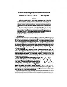
Figure 1: Shell geometry in the reference and the deformed configurations. analysis of thin shells is taken up next. Finally, the excellent performance of the method is established in Section 5 with the aid of selected convergence tests, including the obstacle course of benchmark tests proposed by Belytschko et al. [7].

2 Thin-Shell Boundary Value Problem In this section we summarize the field equations for the classical stress-resultant shell model. A detailed presentation of the classical shell theories can be found in [28]. Here we follow Simo et al. [34, 35] elegant formulation of the Reissner-Mindlin theory, which we specialize to Kirchhoff-Love theory by explicitly constraining the shell director to remain normal to the deformed middle surface of the shell.

2.1 Kinematics of Deformation We begin by considering a shell whose underformed geometry is characterized by a middle surface of domain Ω and boundary Γ = ∂Ω. For simplicity we assume throughout that the thickness h of the shell is uniform. The shell deforms under the action of applied loads and adopts a deformed configuration characterized by a middle surface of domain Ω and boundary Γ = ∂Ω. The position vectors r and r of a material point in the reference and deformed configurations of the shell may be parametrized in terms of a system {θ1 , θ2 , θ3 } of curvilinear coordinates as: r(θ1 , θ2 , θ3 ) = x(θ1 , θ2 ) + θ3 a3 (θ1 , θ2 ),

−

h h ≤ θ3 ≤ 2 2

(1)


5

r(θ1 , θ2 , θ3 ) = x(θ1 , θ2 ) + θ3 a3 (θ1 , θ2 ),

−

h h ≤ θ3 ≤ 2 2

(2)

The functions x(θ1 , θ2 ) and x(θ1 , θ2 ) furnish a parametric representation of the middle surface of the shell in the reference and deformed configurations, respectively (Fig. 1). The corresponding surface basis vectors are: aα = x,α ,

aα = x,α

(3)

where here and henceforth Greek indices take the values 1 and 2, and a comma is used to denote partial differentiation. The covariant components of the surface metric tensors in turn follow as: aαβ = aα · aβ ,

aαβ = aα · aβ

(4)

For later reference we also introduce the contravariant components of the undeformed and deformed surface metric tensors, aαβ and aαβ , respectively. The defining property of these components is: aαγ aγβ = δβα ,

aαγ aγβ = δβα

(5)

We also note that the element of area over Ω follows as √ dΩ = a dθ1 dθ2

(6)

where √ a = |a1 × a2 |

(7)

is the jacobian of the surface coordinates {θ1 , θ2 }. The shell director a3 in the reference configuration coincides with the normal to the undeformed middle surface of the shell and hence has the properties: aα · a3 = 0 ,

|a3 | = 1

(8)

which give a3 explicitly in the form: a3 =

a1 × a2 |a1 × a2 |

(9)

For the moment we allow the director a3 on the deformed configuration of the shell to be an arbitrary vector field. The covariant base vectors in the reference and the current configurations follow simply as gα =

∂r = aα + θ3 a3,α , ∂θα

g3 =

∂r = a3 ∂θ3

(10)

gα =

∂r = aα + θ3 a3,α , ∂θα

g3 =

∂r = a3 ∂θ3

(11)

The corresponding covariant components of the metric tensors in both configurations are: g ij = g i · g j ,

gij = g i · g j

(12)


6

where here and henceforth lowercase Latin indices take the values 1, 2, and 3. The Green-Lagrange strain tensor is defined as the difference between the metric tensors on the deformed and undeformed configurations of the shell, i. e., 1 Eij = (gij − g ij ) 2

(13)

Using equations (10), (11), and (12), the Green-Lagrange strain of the shell is found to be of the form: Eij = αij + θ3 βij

(14)

to first order in the shell thickness h (e. g., [4] pp. 107–112). The nonzero components of the tensors αij and βij are in turn related to the deformation of the shell as follows: 1 αij = (ai · aj − ai · aj ) 2

(15)

βαβ = aα · a3,β − aα · a3,β

(16)

In particular, the in-plane components ααβ , or membrane strains, measure the straining of the surface; the components αα3 measure the shearing of the director a3 ; the component α33 measures the stretching of the director; and the compoments βαβ , or bending strains, measure the bending or change in curvature of the shell, respectively. The above kinematic relations allow for finite deformations as well as for shearing and stretching of the shell director. In the remainder of this paper we restrict our attention to the Kirchhoff-Love theory of thin shells and, accordingly, we constrain the deformed director a3 to coincide with the unit normal to the deformed middle surface of the shell, i. e., aα · a3 = 0,

|a3 | = 1

(17)

which yields a3 =

a1 × a2 |a1 × a2 |

(18)

Owing to these constraints, the shear strains αα3 vanish identically and the bending strains simplify to: βαβ = aα,β · a3 − aα,β · a3

(19)

It follows from these relations that, by virtue of the assumed Kirchhoff-Love kinematics, all the strain measures of interest may be deduced from the deformation of the middle surface of the shell. For simplicity, we restrict the scope of subsequent discussions to linearized kinematics. To this end, we begin by writing x(θ1 , θ2 ) = x(θ1 , θ2 ) + u(θ1 , θ2 )

(20)


7

where u(θ1 , θ2 ) is the displacement field of the middle surface of the shell. To first order in u the membrane and bending strains then follow as: 1 ααβ = (aα · u,β + u,α · aβ ) 2 1 βαβ = −u,αβ · a3 + √ [u,1 ·(aα,β × a2 ) + u,2 ·(a1 × aα,β )] a a3 · aα,β + √ [u,1 ·(a2 × a3 ) + u,2 ·(a3 × a1 )] a

(21)

(22)

It is clear from these expressions that the displacement field u of the middle surface furnishes a complete description of the deformation of the shell and may therefore be regarded as the primary unknown of the analysis. It also follows that the deformed and undeformed domains Ω and Ω are indistinghishable to within the order of approximation of the linearized theory and, in consequence, we drop the distinction between the two domains throughout the remainder of the paper.

2.2 Equilibrium Deformations of Elastic Shells Next, we seek to characterize the equilibrium configurations of the shell by recourse to energy principles. For simplicity, we shall assume throughout that the shell is linear elastic with a strain energy density per unit area of the form: 1 Eh3 1 Eh αβγδ H αβγδ βαβ βγδ W (α, β) = H ααβ αγδ + 2 2 21−ν 2 12(1 − ν )

(23)

where E is Young’s modulus, ν is Poisson’s ratio, and 1 H αβγδ = ν aαβ aγδ + (1 − ν) (aαγ aβδ + aαδ aβγ ) 2

(24)

In (23), the first term is the membrane strain energy density and the second term is the bending strain energy density. The membrane and bending stresses follow from (23) by work conjugacy, with the result: ∂W ∂ααβ ∂W = ∂βαβ

nαβ = mαβ

Eh H αβγδ αγδ 1 − ν2 Eh3 = H αβγδ βγδ 2 12(1 − ν ) =

(25) (26)

The membrane and bending stress tensors nαβ and mαβ may be given a direct mechanistic interpretation as force and moment resultants [18, 34]. The shell is subject to a system of external dead loads consisting of distributed loads q per unit area of Ω and axial forces N per unit length of Γ. Under these conditions the potential energy of the shell takes the form: Φ[u] = Φint [u] + Φext [u]

(27)


where

8

Φint [u] =

W (α, β) dΩ

(28)

Ω

is the elastic potential energy and Φext [u] = −

Ω

q · u dΩ −

Γ

N · u ds

(29)

is the potential energy of the applied loads. The stable equilibrium configurations of the shell now follow from the principle of minimum potential energy: Φ[u] = inf Φ[v] v ∈V

(30)

where V is the space of solutions consisting of all trial displacement fields v with finite energy Φ[v]. It is clear from the form of the elastic energy of the shell that such trial displacement fields must necessarily have square integrable first and second derivatives. Within the context of the linear theory, and under suitable technical restrictions on the domain Ω and the applied loads, it therefore follows that V may be identified with the Sobolev space of functions H2 (Ω, R3 ). In particular, an acceptable finite-element interpolation method must guarantee that all trial finite element interpolants belong to this space. The Euler-Lagrange equations corresponding to the minimum principle (30) may be expressed in weak form as:

DΦ[u], δu = DΦint [u], δu + DΦext [u], δu = 0

(31)

which is a statement of the principle of virtual work. Here DΦ[u], δu denotes the first variation of Φ at u in the direction of the virtual displacements δu,

DΦint [u], δu =

Ω

[nαβ δααβ + mαβ δβαβ ] dΩ

is the internal virtual work and

DΦ [u], δu = −

ext

Ω

q · δu dΩ −

Γ

(32)

N · δu ds

(33)

is the external virtual work. The minimum principle (30) or, equivalently, the virtual work principle (31) are subsequently taken as a basis for formulating finite-element approximations to the equilibrium configuration of the shell.

3 Finite-Element Discretization We now turn to the finite-element discretization of the potential energy of the shell (27) or, equivalently, its first variation (31). To this end, it proves convenient to adopt Voigt’s notation and map symmetric second-order tensors into arrays by recourse to the conventions: 



n11  n=  n22  n12





m11  m=  m22  m12





α11  α =  α22   2α12





β11  β =  β22   2β12

(34)


9

The constitutive relations (Equations 25 and 26) may similarly be written in the form: Eh Hα 1 − ν2

n=

(35)

Eh3 Hβ 12(1 − ν 2 )

m=

(36)

where we write: 

(a11 )2 νa11 a22 + (1 − ν)(a12 )2  (a22 )2 H = sym.



a11 a12  a22 a12  1 11 22 12 2 [(1 − ν)a a + (1 + ν)(a ) ] 2

(37)

which replaces (24) within the Voigt formalism. Using these conventions, the internal virtual work (32) may be recast in the convenient form

Φint [u], δu =

Ω

Eh Eh3 T δβ T Hβ dΩ δα Hα + 1 − ν2 12(1 − ν 2 )

(38)

Next we proceed to partition the domain Ω of the shell into a finite element mesh, the precise nature of which will remain unspecified for now. The collection of element domains in the mesh is {ΩK , K = 1, . . . , NEL}, where ΩK denotes the domain of element K and NEL is the total number of elements in the mesh. The finite-element mesh may be taken as a basis for introducing a displacement interpolation of the general form: 1

2

uh (θ , θ ) =

NP

N I (θ1 , θ2 )uI

(39)

I=1

where {N I , I = 1, . . . , NP } are the shape functions, {uI , I = 1, . . . , NP } are the corresponding nodal displacements, and NP is the number of nodes in the mesh. Owing to the linearity of the dependence of the finite-element interpolant uh on the nodal displacements, an application of (21) and (22) to (39) gives the finite-element membrane and bending strains in the form: αh (θ1 , θ2 ) = β h (θ1 , θ2 ) =

NP

I=1 NP

M I (θ1 , θ2 )uI

(40)

B I (θ1 , θ2 )uI

(41)

I=1

for some matrices M I and B I . The precise form of this matrices is given in Appendix A.0.3. Finally, the introduction of (39), (40) and (41) into the principle of virtual work (31) yields the equations of equilibrium for the nodal displacements: K h uh = f h

(42)

where, by a slight abuse of notation, here we take uh to signify the array of nodal displacements, K IJ h

=

N

EL K=1

ΩK

N

EL Eh Eh3 I T J I T J (M ) HM + (B ) HB dΩ ≡ K IJ K (43) 2 2 1−ν 12(1 − ν ) K=1


10

is the stiffness matrix, and f Ih =

N

EL ΩK

K=1

qN I dΩ +

ΓK ∩Γ

N N I ds ≡

N

EL

f IK

(44)

K=1

is the nodal force array. It should be carefully noted that, as expected, the global stiffness and force arrays just defined follow by the assembly of low-dimensionality element stiffness and I force arrays K IJ K and f K , respectively, as is standard in the finite-element method. The computation of element arrays requires the evaluation of integrals extended to the domain of each element, cf. Equations (43), (44). These integrals may efficiently be evaluated by recourse to numerical quadrature without compromising the order of convergence. For instance, the application of a quadrature rule to the calculation of the element stiffness matrices leads to the expression: K IJ K

=

NQ

G=1

Eh3 Eh I T J (B I )T HB J (M ) HM + 1 − ν2 12(1 − ν 2 )

1 2 a(θG , θG )wG (45)

1 ,θ 2 ) (θG G

1 2 where (θG , θG ) are the quadrature points, wG are the corresponding quadrature weights, and NQ is the number of quadrature points in the rule. The element force arrays f IK may be computed likewise. Sufficient conditions for the quadrature rule to preserve the order of convergence of the finite-element method may be found in [40]. In general, this conditions demand that certain shape function derivatives be computed exactly and, consequently, place a lower bound on the order NQ of the quadrature rule. These theoretical considerations and our numerical tests show that a one-point quadrature rule is sufficient to compute all element arrays of interest.

4 Subdivision Surfaces and Finite-Element Interpolation It is clear from the preceding developments that the central problem in thin-shell finite-element analysis is the formulation of shape functions N I which are H 2 (or ‘C 1 ’ in the usual finiteelement terminology), as this property ensures the finiteness of the energy of the trial displacement fields. In this section we develop one such interpolation scheme based on the notion of subdivision surface.

4.1 Subdivision Surfaces We begin by reviewing the essential ideas behind subdivision surfaces using one-dimensional examples first, then moving to the two-dimensional manifold (with boundary) setting relevant to shells. Here we limit ourselves to reviewing various elementary properties of subdivision. The interested reader is referred to [29, 33, 45, 46] for more details and further pointers to the literature. Throughout this discussion the term vertex will be used to refer to nodes in the mesh. For example, a vertex has associated with it a particular nodal position. A vertex has a topological neighborhood defined by the structure of the mesh. For example, its 1-ring neighbors are all those vertices which share an edge with it (and recursively for its k-ring). This distinction


11

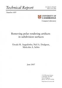
between vertices and nodal positions is typically not needed when dealing with finite elements, but it is important to keep these distinctions in mind when dealing with smooth subdivision. At the highest level of description we may say that subdivision schemes construct smooth surfaces through a limiting procedure of repeated refinement starting from an initial mesh. This initial mesh will also be referred to as the control mesh of the surface. Generally, subdivision schemes consist of two steps. First the mesh is refined, e.g., all faces are quadrisected, followed by the computation of new nodal positions. These positions are simple, linear functions of the nodal positions of the coarser mesh. For the schemes of interest these computations are local, i.e., they involve only nodal positions of the coarser mesh within a small, finite topological neighborhood, leading to very efficient implementations. Using a suitable choice of weights, such subdivision schemes can be designed to produce a smooth surface in the limit. Subdivision methods which result in limit surfaces whose curvature tensor is square integrable are especially appealing for geometrical modeling applications and for the purpose of thin-shell analysis. The first such schemes were proposed by Catmull and Clark [12] and Doo and Sabin [15]. Since then, many other schemes have been proposed and studied extensively in the mathematical geometric modeling literature. The methods can be separated into two groups: • Interpolating Schemes: The nodal positions of the coarser mesh are fixed, while only the nodal positions of new vertices are computed when going from a coarser to a finer mesh. Consequently, the nodal positions of the initial mesh, as well as any nodes produced during subdivision, interpolate the limit surface. Interpolating schemes for quadrilateral meshes have been introduced by Kobbelt et al. [24], while Dyn et al. [16] and Zorin et al. [47] described interpolating schemes for triangular meshes. In both cases the limit surfaces are C 1 but their curvatures do not exist. Therefore, these schemes are not suitable for the special application of thin-shell analysis. • Approximating Schemes: These schemes compute both new nodal positions for the newly created vertices, as well as for the vertices inherited from the coarser mesh, i.e., those which already carried nodal positions. Consequently, the nodal positions of the initial mesh are not samples of the final surface. The schemes of Catmull-Clark [12] and Doo-Sabin [15] fall into this class and operate on quadrilateral meshes. An approximating scheme for triangular meshes introduced by Loop [26] is used in the present work. This scheme produces limit surfaces which are globally C2 except at a number of isolated points where they are only C 1 . However, their principal curvatures are square integrable [30], making them good candidates for thin-shell analysis. A simple one-dimensional example of an approximating as well as an interpolating scheme is shown in Figure 2. We assume that the polygon with the nodes xkI is the result of subdivision step k. In the subsequent refinement k + 1 for the approximating scheme, a new vertex gets a k k nodal position xk+1 2I+1 which is the average of its two neighboring nodes xI and xI+1 : 1 k k xk+1 2I+1 = (xI + xI+1 ) 2

(46)

The nodal positions of the existing vertices are recomputed as xk+1 2I =

1 k xI−1 + 6xkI + xkI+1 8

(47)


12

Since throughout the subdivision process all nodal positions are recomputed as weighted averages of nearby vertices, the resulting scheme does not interpolate the nodal positions of the control mesh, but rather approximates them. In contrast, the interpolating scheme (see Figure 2) does not modify the coordinates of nodes existing at the previous refinement level: k xk+1 2I = xI

(48)

Only the newly generated vertices receive new nodal coordinates: xk+1 2I+1 =

1 k −xI−1 + 9xkI + 9xkI+1 − xkI+2 16

(49)

Repeating this process ad infinitum leads to smooth curves. In the case of the approximating scheme above, these curves are actually cubic splines which are C2 continuous. The interpolating scheme on the other hand is known as the 4pt scheme, and it can be shown that the resulting curves are C 2− continuous [14]. Since the entire subdivision process is linear, the resulting limit curves (or surfaces) are linear combinations of basis functions (sometimes referred to as ‘fundamental solutions’ of the subdivision process). The compact support of the subdivision rules ensures that the basis functions are compactly supported as well. For the approximating scheme above, this support extends two vertices to the left and two vertices to the right (and hence is a 2-ring), while the 4pt scheme has a support covering three vertices to each the left and right (hence a 3-ring). Both schemes belong to the class of regular subdivision schemes since the weights are the same for every vertex and every level. In the two-dimensional case, we will see that the weights will depend on the valence, i.e., the number of edges attached to a vertex, but are otherwise the same from level to level. These rules are also referred to as semi-regular. Similarly one can adapt the rules to non-smooth features such as boundaries or creases [19], as well as other boundary conditions [8]. In the one-dimensional case, subdivision schemes do not offer an important advantage since curves of the desired smoothness are easy to construct with traditional approaches such as Hermitian interpolation. In the two-dimensional, arbitrary-topology manifold setting, by contrast, subdivision methods offer significant advantages over other methods of smooth-surface construction. In fact, their original invention was motivated by the difficulties of constructing smooth-surface models of arbitrary-topology. For example, it is well known that C2 arbitrarytopology surfaces built with traditional patches require up to sixth-order polynomials, leading to cumbersome computations and difficult-to-manage cross-patch continuity conditions. Additionally, the resulting degrees of freedom often lack physical meaning. In the subdivision setting however, the only degrees of freedom are the nodal positions and the resulting surfaces are guaranteed to be smooth without the need to enforce cross-patch continuity conditions. In the following sections we introduce the refinement rules used in Loop’s subdivision scheme for surfaces; and, based on the concept of the subdivision matrix, briefly discuss the basic ideas behind the scheme’s smoothness analysis. This discussion will serve to prepare the way for the parameterization of subdivision surfaces needed for the evaluation of positions, tangents, and curvatures. In particular, it is possible to evaluate these quantities exactly through the use of eigenanalysis without going to the limit. While we focus on Loop’s scheme, we hasten to point out that the basic ideas and machinery apply equally well to other subdivision schemes. In particular, the Catmull-Clark scheme, with quadrilateral elements, is a promising alternative


13

first subdivision step

initial polygon

second subdivision step

Figure 2: Two subdivision methods: approximating (first row) and interpolating (second row). Valence of a vertex Regular vertex Irregular vertex One ring of a vertex One ring of an element

: : : : :

The number of element edges attached to a vertex Vertex with valence six Vertex with valence unequal to six Set of vertices incident to the vertex Set of elements incident to the element

Figure 3: Summary of frequently used terms in the case of triangle meshes

for finite-element computations, since quadrilateral elements generally perform relatively better for very coarse meshes.

4.2 Refinement Rules In Loop’s subdivision scheme, the control mesh and all refined meshes consist of triangles only. These are refined by quadrisection (Fig. 4). After the refinement step, the nodal positions of the refined mesh are computed as weighted averages of the nodal positions of the unrefined mesh. We distinguish two cases: new vertices associated with the edges of the coarser mesh, and old vertices of the coarse mesh. The coordinates of the newly generated nodes x11 , x12 , x13 , · · · on the edges of the previous mesh are computed as: xk+1 = I

3xk0 + xkI−1 + 3xkI + xkI+1 8

I = 1, . . . , N

(50)

whereby index I is to be understood in modulo arithmetic. The old vertices get new nodal


14

00x3 11 0

0 x00 4 11

x14

0 00 x11 5 00 11

1 0 00 1

1 0 0 1

11 0 x00

x15

x2

x00

x16

11 00 000 11

6

1 0

00 x111 1 0 00 0311 1

1 0 x12 0 0 1 1 x10 00 11 00 11 x11

x1

Figure 4: Refinement of a triangular mesh by quadrisection. positions according to: = (1 − Nw)xk0 + wxk1 + · · · + wxkN xk+1 0

(51)

where xk are the nodal positions of the mesh at level k and xk+1 are the respective positions for the mesh k + 1. The valence of the vertex, i.e., the number of edges incident on it, is denoted by N. Note that all newly generated vertices have valence 6 while only the vertices of the original mesh may have valence other than 6. We will refer to the former case (valence = 6) as regular and to the latter case as irregular. The eqs. 50 and 51 are visualized in symbolic form in Figure 5 with the so-called subdivision mask. At this stage it is not obvious how to choose the parameter w to get C 1 continuous surfaces. In the original scheme Loop [26] proposed

1 5 3 1 2π w= − + cos N 8 8 4 N

2

.

(52)

As it turns out other values for w also give smooth surfaces. For example, Warren’s [42] choice for w is simpler to evaluate than that of Equation 52: w=

3 8N

for N > 3

w=

3 16

for N = 3

(53)

Although the choice for the weights appears somewhat arbitrary, the motivation for this choice will be discussed in the next section. In any case, the weights used by the subdivision scheme depend only on the connectivity of the mesh and are independent of the nodal positions. So far we have ignored the boundary of the mesh, where the subdivision rules need to be modified. Two choices are possible here. The first method considers the boundary as a one-dimensional curve and applies the rules of Equations (46) and (47) to any vertices on the boundary (see [19]). Another method for the treatment of boundaries, which we employ in our implementation, was proposed by Schweitzer [33]. For each boundary edge, one temporary vertex is defined, after which the ordinary rules are applied. The nodal positions of the temporary vertices are set to (see Figure 6) : x03 = x00 + x02 − x01

and

x04 = x00 + x05 − x06 .

(54)


15

w

1 8

w

w

11 00 00 11 00 11

3 8

1 − Nw w

3 8

w 1 8

w

Figure 5: Refinement mask for Loop’s subdivision scheme.

x04

11 00

11 00 00 11

x00

x05

1 0 0 1

11 00

0

x3 11 00 00 11 x02

1 0

1 0 x1 11 00 00 11 0

1 0

x06

11 00

1 0 0 1

Figure 6: Smooth boundary approximation with artificial nodes.


16

Figure 7: Distributor cap: Control mesh, first subdivided mesh, and the resulting limit surface (original data courtesy Hugues Hoppe). This particular choice of temporary vertices effectively reproduces the one-dimensional subdivision rules. This simplified boundary treatment with temporary vertices leads to approximation errors for corners and boundary vertices with valence other than 4. However, these errors do not inhibit the convergence of the finite-element method. For modeling surfaces with creases or shell intersections, the edge rules can also be applied within the mesh on appropriately tagged edges. Figure 7 shows an example of a geometrically more complex shape, a distributor cap, using such crease rules, demonstrating the ability of subdivision surfaces to model intricate shapes in a straightforward fashion. The entire shape is a single, piecewise smooth surface. In this example, the original mesh is chosen to be least-squares optimal in terms of geometric approximation fidelity. For finite-element simulations, this triangulation first needs to be improved to ensure a uniform aspect-ratio bound. Algorithms for performing this task have been described by Kobbelt et al. [23]. In instances where the original geometry is given in some other form, a remeshing step can be applied to produce high-quality subdivision meshes, as demonstrated by Lee et al. [25].

4.3 Convergence and Smoothness Subdivision methods for arbitrary-topology surfaces were introduced more than 20 years ago, but not widely used in applications until the early 1990s when theoretical breakthroughs put their convergence and smoothness analysis on a solid mathematical foundation [29, 33, 45]. If all vertices are regular (valence 6 for triangles or valence 4 for rectangular schemes), powerful Fourier methods can be used to establish smoothness properties. These techniques do not apply in the arbitrary-topology manifold setting, in which irregular vertices cannot be avoided. The critical question in this setting concerns the smoothness properties around irregular vertices. The key tool in this analysis is the local subdivision matrix and its structure. The fact that the analysis of these schemes can be reduced to the analysis of a local matrix is due to the local support of the basis functions. In other words, the behavior of the surface in a neighborhood of a node depends only on those basis functions whose support overlaps a neighborhood of the node.


17

For Loop’s scheme, the relevant neighborhood around a vertex is a 2-ring, i.e., all vertices which can be reached by traversing no more than two edges. The subdivision matrix expresses the linear relationship between the nodal positions in a 2-ring around a given vertex at level k and the nodal positions around the same vertex in the 2-ring at level k + 1. This 2-ring analysis is required to establish smoothness. Details of this approach, including necessary and sufficient conditions, can be found in Reif [29], Zorin [45], and Schweitzer [33]. Once the analytic properties have been established, quantities at a point, such as position or tangents, can be computed using an even smaller subdivision matrix which relates 1-rings at level k to those at level k + 1. In the following we will discuss only this simpler setting since it is the one which is needed for actual computations. Let X k be the vector of nodal positions of a vertex with valence N and its 1-ring neighbors at level k, X k = (xk0 , xk1 , . . . , xkN ). Note that in the surface case we treat this vector as an N +1 vector of three-dimensional vectors, while in the functional setting it would be an N + 1 vector of scalars. We can now express the linear relationship between the nodal positions at level k and k + 1 with an (N + 1) × (N + 1) matrix S: X k+1 = SX k

(55)

The entries of the matrix S are given by the subdivision rules (Equations 51 and 50). The study of the limit surface then amounts to examining X ∞ = lim S k X 0

(56)

k→∞

From this it immediately follows that the limit surface cannot exist if S has an eigenvalue of modulus larger than 1. Furthermore, it can be shown that it must have a single eigenvalue 1 and all other eigenvalues must have modulus strictly smaller than 1. This property also implies that subdivision schemes are affinely invariant, i.e., an affine transformation applied to the nodal positions of the control mesh results in a limit surface having undergone the same affine transformation, which is a desirable property in practical applications. The associated right eigenvector is easily seen to be the vector of all 1’s. In the following we summarize the main results as needed for our finite-element setting. Assume that the subdivision matrix has a complete set of eigenvectors (this property holds for all schemes of practical interest, although it is not necessary for the analysis). Since the subdivision matrix S is not self-adjoint, let RI and LJ be the right and left eigenvectors of S respectively, LJ · RI = δIJ

(57)

and let λI be the associated eigenvalues in non-increasing magnitude order, with λ0 = 1. Using the eigenvalue decomposition, the nodal vector X 0 can be written as X0 =

N

a0I RI

(58)

I=0

with a0I = LI · X 0 . Choosing this basis, Equation (56) takes the simple form: X

∞

= lim S k→∞

k

N

I=0

a0I RI

= lim

k→∞

N

I=0

λkI a0I RI

(59)


18

tangent masks

position mask

l l

c4 l

cN

l

s3

s5

0 l

l

c3

c5

1 − Nl

s4

0 c2

s2

sN

c1

s1

Figure 8: Limit masks for Loop’s subdivision scheme. From this representation and the facts that λ0 = 1 and |λI | < 1 for I = 1, . . . , N, it follows immediately that the center nodal position as well as all nodal positions in the 1-ring converge to X ∞ = a00 R0

(60)

Since R0 has the form R0 = (1, 1, · · · , 1) all the nodal positions in the 1-ring neighborhood actually converge to a single position: a00 = L0 · X 0

(61)

For the original Loop subdivision scheme, L0 is given as L0 = (1 − Nl, l, · · · , l)

with l =

1 . 3/(8w) + N

(62)

In practical terms this means that we can evaluate the limit position of the surface given at any finite subdivision level by simply applying the mask shown in Figure 8. We can continue this analysis and compute tangent vectors in a similar way. Assume that the control nodal positions have been translated by −a0 so that the limit position for our selected vertex is the origin. The leading term of Equation (59) is now controlled by the subdominant eigenvalues. Here we have λ1 = λ2 > λ3 , which results in Xk = a01 R1 + a02 R2 k→∞ λk 1 lim

(63)

indicating that the nodal positions in the 1-ring all converge to a common plane spanned by the vectors a01 and a02 . While these vectors are not necessarily orthogonal, they do span a plane for almost all initial configurations. An explicit formula for two tangent vectors to the limit surface is: t1 = L1 · X 0

t2 = L2 · X 0

whence the shell director follows as: t1 × t2 a3 = |t1 × t2 |

(64)

(65)


19

9

5

10

11

12

1111111 0000000 0000000 1111111 0000000 1111111 7 8 0000000 1111111 0000000 1111111 0000000 1111111 0000000 1111111 0000000 1111111 0000000 1111111 4

2

6

3

1

Figure 9: A regular box-spline patch with 12 control points. In certain settings we may have λ1 ≥ λ2 > λ3 , as pointed out by Schweitzer [33]. The above equations for tangent vectors continue to hold, requiring an argument only slightly more involved than the one above. For Loop’s scheme, L1 , L2 are given by L1 = (0, c1 , c2 , · · · , cN )

L2 = (0, s1, s2 , · · · , sN )

(66)

with cI = cos

2π(I − 1) N

sI = sin

2π(I − 1) . N

Again we find that a very simple computation (see the masks in Figure 8) allows us to compute the limit surface normal given the subdivision mesh at any level k. So far we have only discussed the evaluation of position and tangents of the limit surface at parametric locations corresponding to control vertices. For numerical evaluation of the Kirchhoff-Love energy functional we need to evaluate these quantities — and curvature quantities — at quadrature points. This is particularly simple in the case of Loop’s scheme (and similarly so for Catmull-Clark’s scheme) since Loop’s scheme actually generalizes quartic box splines (Catmull-Clark’s scheme generalizes bi-cubic splines). If the valencies of the vertices of a given triangle are all equal to 6, the resulting piece of limit surface is exactly described by a single quartic box-spline patch, for which very efficient evaluation schemes exist at arbitrary parameter locations. We call such a patch regular (see Fig. 9). Regular patches are controlled by 12 basis, or shape, functions (see Appendix A.0.1), since only their support overlaps the given patch. If a triangle is irregular, i.e., one of its vertices has valence other than 6 the resulting patch is not a quartic box spline. Arbitrary parameter locations may nevertheless be treated simply by the method described in the next section.

4.4 Function Evaluation for Arbitrary Parameter Values In this section we discuss the evaluation of function values and derivatives for Loop subdivision surfaces at arbitrary parameter locations. These function evaluations arise during the computation of element stiffness and force arrays by numerical quadrature, Equation (45). Despite


20

early attempts [12], the proper parameterization of subdivision surfaces has been until recently an unsolved problem in the vicinity of irregular vertices. Stam [39, 38] presented an elegant solution to this problem based on the eigendecomposition of the subdivision matrix. A convenient local parameterization of the limit surface may be obtained as follows. For each triangle in the control mesh we choose (θ1 , θ2 ) as two of its barycentric coordinates within their natural range T = {(θ1 , θ2 ), s. t. θα ∈ [0, 1]}

(67)

The triangle T in the (θ1 , θ2 )-plane may be regarded as a master or standard element domain. It should be emphasized that this parameterization is defined locally for each element in the mesh. The entire discussion of parameterization and function evaluation may therefore be couched in local terms. Consequently we proceed to consider a generic element in the mesh and introduce a local numbering of the nodes lying in its immediate 1-neighborhood. For regular patches such as depicted in Figure 9, Loop’s scheme leads to classical quartic box splines. Therefore, the local parameterization of the limit surface may be expressed in terms of box-spline shape functions, with the result: x(θ1 , θ2 ) =

12

N I (θ1 , θ2 )xI

(68)

I=1

where now the label I refers to the local numbering of the nodes. The precise form of the shape functions N I (θ1 , θ2 ) is given in Appendix A.0.1. The surface within the shaded triangle in Figure 9 is controlled by the 12 local control vertices. In contrast to Hermitian interpolation, the surface is solely controlled by the position of these control vertices, and first- or second-order derivatives at the nodes are not utilized. The image of the standard domain T under the embedding (68) constitutes the geometric domain of the element under consideration within the limit surface. The embedding (68) may thus be regarded as a conventional isoparametric mapping from the standard domain T onto Ω, with (θ1 , θ2 ) playing the role of natural coordinates. The parameterization in Equation 68 may also be used for the displacement field. Locally one then has uh (θ1 , θ2 ) =

12

N I (θ1 , θ2 )uI

(69)

I=1

For function evaluation on irregular patches the mesh has to be subdivided until the parameter value of interest is interior to a regular patch. At that point the regular box-spline parameterization applies once again. It should be noted that the refinement is performed for parameter evaluation only. For simplicity we assume that irregular patches have one irregular vertex only. This restriction can always be met for arbitrary initial meshes through one step of subdivision, which has the effect of separating all irregular vertices. Figure 10 illustrates the basic idea for arbitrary parameter evaluation. It shows an irregular patch (center) with a single vertex of valence 7. After one level of subdivision this patch is divided into four patches, three of which are regular. If the desired parameter value lies within those patches we may immediately evaluate the surface by using the canonical regular-patch evaluation routine. If our desired parameter location lies within the fourth sub-patch, we must


N+5

21

N+2

N+6

N+1

N

N+3

2

1

N+4

11 00 00 11 00 11 00 111 211 3 00 00 11 00 11 00 11

3

4 5

Patch 2

Patch 1

11111111 00000000 00000000 11111111 1

2

Figure 10: Refinement near an extraordinary vertex.

Patch 3

3


22

2

1

3 1.

5

5

0.

0.

0

2

0

1 1.

3

Figure 11: Refinement in the parameter space. repeatedly subdivide until it falls within a regular patch. This can be achieved for any parameter value away from the irregular vertex. As shown in Figure 10, after one subdivision step the triangles marked one, two, and three are regular patches. The action of the subdivision operator for this entire neighborhood can again be described by a matrix: X 1 = AX 0

(70)

The matrix A now has dimension (N + 12, N + 6) and its entries can be derived from the subdivision rules as presented in Section 4.2. For the proposed shell element with one-point quadrature at the barycenter of the element, a single subdivision step is sufficient, since the sampling point (center of the initial patch) lies in sub-patch 2. We define 12 selection vectors P I , I = 1, . . . , 12 of dimension (N + 12) which extract the 12 box-spline control points for sub-patch 2 from the N + 12 points of the refined mesh. The entries of P I are zeros and one depending on the indices of the initial and refined meshes. To evaluate the function values in the three triangles with the box-spline shape functions N I , a coordinate transformation must be performed. The relation between the coordinates (θ1 , θ2 ) of the original triangles and the coordinates (θ˜1 , θ˜2 ) of the refined triangles can be established from the refinement pattern in Figure 11. For the center of sub-patch 2 we have the following relation: Triangle 2:

θ˜1 = 1 − 2θ1

θ˜2 = 1 − 2θ2

(71)

The function values and derivatives for sub-patch 2 can now be evaluated using the interpolation rule: x(θ1 , θ2 ) =

12

N I (θ˜1 , θ˜2 )P I AX 0

(72)

I=1

Differentiation of the above equation yields the partial derivatives of x at the desired location. In these calculations, the jacobian matrix of the simple mapping (72) between the coordinates (θ1 , θ2 ) and (θ˜1 , θ˜2 ) has to be included. The result is: x,α (θ1 , θ2 ) = −2

12

I=1

N I ,α (θ˜1 , θ˜2 )P I AX 0 ≡ aα (θ1 , θ2 )

(73)


23

displacements and rotations fixed

displacements and rotations free

displacements fixed rotations free

11 00 00 11

U4 = U2 + U3 − U1

U4 = −U1

11 00 00 11

U4 = 0

U2 = 0 00 11

00 11 U1 = 00 0 11

U3 = 0

11 00

U11 2 00

00 11

U3

11 00

U1 00 11

11 00 00 11

U2 =11 0 00

00 11

U1

U3 = 0

1 0

11 00

Figure 12: Boundary conditions. The jacobian of the embedding required in the quadrature rule (45) can in turn be computed directly from aα through (7). Second-order derivatives such as required for the computation of bending strains follow simply by direct differentiation of the interpolation rule (73). The evaluation procedure just described is a simplified version of the scheme presented by Stam [38] for function evaluation at arbitrary parameter values. Since we are only interested in a one-point quadrature rule, a single subdivision step is sufficient. For other rules one may need to subdivide further. Stam describes the general case in which the eigendecomposition of A is exploited to perform the implied subdivision steps through suitable powers of A in the eigenbasis, a simple and efficient procedure.

4.5 Dirichlet Boundary Conditions Due to the local support of the subdivision scheme, the boundary displacements are influenced only by the nodal positions in the 1-neighboorhood of the boundary, i. e., the first layer of vertices inside the domain as well as a collection of artificial or ‘ghost’ vertices just outside the domain. For example, for built-in boundary conditions the displacements of the nodes inside, outside, and on the boundary must be zero (see Figure 12). The deformation of the boundary computed with the limit formula as described in Section 4.3 shows that this results in zero displacements and in fixed tangents. Other boundary conditions can be accommodated in a similar way (see Figure 12). The enforcement of prescribed boundary displacements is equally straightforward. General displacement boundary conditions may be formulated with the aid of a local reference frame defined by the surface normal and the tangent to the boundary of the shell. The prescribed displacement boundary conditions may be regarded as linear contraints on the displacement field and treated accordingly during the solution process. Such linear constraints may be enforced by a variety of methods [11]. In all the calculations reported here, the displacement boundary conditions are enforced by the penalty method, with a penalty stiffness equal to 100 times the maximum diagonal component of the stiffness matrix.


24

4.6 Implementation of Subdivision-Based Shell Elements We close this section with selected remarks on matters of implementation. The implementation of the element requires a few data structures in addition those typical of the conventional finite element method. For example, tables of element adjacencies are needed for the computation of element arrays. In our implementation, we use a Triangle C-structure which stores the following information for each element of the mesh: typedef struct _T { /* pointer to the element vertices */ /* pointer to the neighbor triangles */ /* array of pointers to the vertices in the 1-neighborhood */ /* number of nodes in the 1-neighborhood */ /* information about the boundary conditions of the edges */ } Triangle; The solution process consists of the following steps: 1. Subdivide the initial mesh once in order to separate the irregular vertices (the initial mesh could include triangles with more than one irregular vertex — in order to limit the number of possible mesh patterns during the parameter evaluation, we refine the mesh once so that each triangle has at most one irregular vertex). 2. Generate artificial nodes and elements at the boundaries (see Section 4.2). 3. Find the 1-neighborhood of each element and gather the local nodes in accordance with the local numbering convention. 4. Create local coordinate systems at the nodes if necessary. For the creation of the local coordinate systems, we employ the limit formula of Equation (65) for the shell normal. 5. Compute and assemble the element stiffness matrices and force arrays. 6. Introduce displacement boundary condition constraints (see Section 4.5). 7. Solve the system of equations. 8. Compute the limit positions of the nodes, Equation (60). The elements under consideration here have three nodes and three displacement degrees of freedom per node. We use one-point quadrature with the sole quadrature point in the rule 1 2 = 1/3 and θG = 1/3. The corresponding located at the barycenter of the element, i. e., at θG weight is w = 1/2, which, evidently, is the area of the standard triangle T . In sum, the preceding developments lead to the definition of a class of fully conforming 1 ‘C ’ triangular elements containing three nodes and one quadrature point. This combination of attributes, namely, the low order of interpolation and quadrature required, render the element particularly attractive from the standpoint of computational efficiency. As mentioned earlier, subdivision surfaces may also be used to define four-node square shell elements, but this extension of the method will not be pursued here.


25

5 Examples We proceed to establish the convergence characteristics of the method by running the obstacle course of test cases proposed by Belytschko et al. [7]. The shells in these tests cases take simple spherical or cylindrical shapes which can be readily described analytically. A preliminary step in the calculations is to approximate the exact surface of the shell by a subdivision surface. Several methods of approximation are possible, including: 1. Least-squares approximation of the exact surface by the limit surface; 2. Placement of the control-mesh nodes on the exact surface; and others. However, theoretical considerations and our own numerical tests show that the error incurred in the approximation of the shell geometry is of higher order than the finiteelement error, and consequently both methods of approximation result in the same convergence rates asymptotically. It should also be noted that the question of geometrical approximation is rendered moot within an integrated computer-aided geometrical design (CAGD) — finiteelement analysis framework. In this environment, the subdivision surface generated by the CAGD module becomes the true shell surface to be analyzed by the finite-element analysis module. We note for further reference that a strictly C1 finite-element method for Kirchhoff-Love shell theory containing the complete set of third-order polynomials within its interpolation satisfies the error bound [13]: uh − u2,Ω ≤

C |u|3,Ω NP

(74)

where u is the exact solution, uh is the finite-element solution, C is a constant, NP is the number of nodes in the mesh, · 2,Ω is the standard norm over H 2 (Ω; R3 ), or ‘energy norm’, and | · |3,Ω is the standard semi-norm over H 3 (Ω; R3 ). The central question to be ascertained now is whether the method developed in the foregoing exhibits the optimal convergence rate implied by the bound (74). All the calculations described subsequently are carried out with one-point quadrature. The successive mesh refinements considered in convergence studies are obtained by regular refinement. We additionally compare the performance of the proposed approach with that of two other shell elements: ASM : The assumed-strain four-noded shell element of Simo et al. [35]. DKT-CST : A flat 3-node element with no membrane/bending coupling [17]. In this element the discrete Kirchhoff triangle (DKT) formulation of Batoz [5] is utilized for the bending response, and standard constant strain interpolation is used for the membrane response. The resulting element has six degrees of freedom per node.

5.1 Rectangular Plate As a first example, we consider the simple case of a square plate under uniform loading p = 1, Fig. 13. The length of the plate is L = 100 and the thickness is h = 1. These dimensions place


26

L

Geometry:

L = 100.0 h = 1.0

Material properties: E = 1.0 · 107 ν = 0.0 Uniform loading

p = 1.0

L Figure 13: Definition of the plate test problem and a typical mesh used in the calculations.

Figure 14: Calculated deformed shapes for the clamped and simply-supported plates (deflections scaled differently in both cases). the plate well within the scope of Kirchhoff’s theory. The Young’s modulus is E = 107 and the Poisson’s ratio is ν = 0. In order to test the treatment of displacement boundary conditions described in Section 4.5, we analyze both a simply-supported and a clamped plate. The entire plate is discretized into finite elements with no account taken of the symmetry of the plate. A typical mesh used in the calculations is shown in Fig. 13. The artificial or ghost nodes used to enforce the boundary conditions are not shown in the figure. The computed limit surfaces of the simply-supported and clamped plates following deformation are shown in Figure 14. The high degree of smoothness of these deflected shapes is noteworthy. An appealing feature of the problem under consideration is that it is amenable to an exact analytical solution. For instance, the maximum displacement at the center of the plate is found to be: umax ≈ 0.487 for the simply-supported plate; and umax ≈ 0.151 for the clamped plate [41]. It therefore follows that the solution error can be computed exactly for this problem. The computed maximum-displacement and energy-norm errors are shown in Figure 15 as a function of the number of degrees of freedom. In all cases, the optimal convergence rate O(NP −1) is attained in the energy norm, which attests to the good convergence properties of the method. These results, and those presented subsequently, also demonstrate the sufficiency of the one-point quadrature rule.


1.4 simple supported fixed

Normalized max. displacement

Relative error in energy norm

100

27

10

1

0.1

0.01 10

100 1000 10000 Number of degrees of freedom

simple supported fixed

1.3 1.2 1.1 1 0.9 0.8 0.7 0.6

0

400 800 1200 1600 Number of degrees of freedom

2000

Figure 15: Convergence of the energy and maximum-displacement errors for the simplysupported and clamped plate problems. Geometry:

L R

R

2θ

L = 50.0 R = 25.0 h = 0.25 θ = 40deg

Material properties: E = 4.32 · 108 ν = 0.0 Gravity load

p = 90.0

Figure 16: Definition of Scordelis-Lo problem.

5.2 Scordelis-Lo Roof The Scordelis-Lo Roof is a membrane-stress dominated problem and, as such, it provides a useful test of the ability of the finite-element element method to represent complex states of membrane strain. The problem concerns an open cylindrical shell loaded by gravity forces, Figure 16. In our calculations, the length of the cylinder is L = 50; its radius is R = 25; the angle subtended by the roof is φ = 80deg ; the thickness is h = 0.25; the Young’s modulus is E = 4.32 · 108 ; and the Poisson’s ratio is ν = 0. The undeformed control mesh and the deformed limit surface are shown in Figure 5.2. A convergence plot for the maximum displacement is shown in Figure 18. The displacements are normalized by the value 0.3024 as given in [7]. The excellent convergence characteristics of the method are evident from the figure. In particular, the subdivision element outperforms both the assumed-strain and the DKT elements.


28

Figure 17: Scordelis-Lo Roof: typical control mesh; deformed limit surface.

Normalized maximum displacement

1.4

Present ASM DKT

1.3 1.2 1.1 1 0.9 0.8 0.7 0.6

0

500

1000 1500 2000 2500 3000 3500 Number of degrees of feedom

Figure 18: Displacement-convergence plot for Scordelis-Lo Roof.


00 11 0 1 0 1 0 1 0 1 0 L/2 1 0 1 0 1 0 1 0 1 111 000 0 1 0 F 1 0 1 0 1 0 1 0 L/2 1 0 1 0 1 0 1 00 11 0 1 00 11 0 1 0 1 01 1 0 1 00 11 0 1 00 11 0 0 1 0 1 0 1 00 11 00 11 0 1 0 1 01 1 0 1 00 11 0 1 00 11 0 00 11 0 1 0 1 0 1 11 00 0 1 00 11 00 11 0 1 0 1 00 11 0 1

29

R

F

Geometry:

L = 600.0 R = 300.0 h = 3.0

Material properties:

E = 3.0 · 106 ν = 0.3

Concentrated forces:

F = 1.0

Figure 19: Definition of the pinched-cylinder problem.

Figure 20: Pinched-cylinder problem: typical control mesh; deformed limit surface.

5.3 Pinched Cylinder The pinched-cylinder problem tests the method’s ability to deal with inextensional bending modes and complex membrane states. The problem concerns a cylindrical shell pinched under the action of two diametrically opposite unit loads located within the middle section of the shell. We consider two cases: free-end boundary conditions; and ends constrained by two rigid diaphragms. The length of the cylinder is L = 600; the radius is R = 300; the thickness is h = 3; the Young’s modulus is E = 3×106 ; and the Poisson’s ratio is ν = 0.3. A control-mesh node is placed at the point of application of the loads. It is interesting to note, however, that, owing to the nonlocal character of the shape functions, the point load is spread over several nodes. This is in contrast to other methods, e. g., those based on Hermitian interpolation. It should be carefully noted that the shape functions developed here possess the requisite partitionof-unity property and, in consequence, the resultant of all nodal forces exactly matches the applied load.

30

Present ASM DKT

1.2 1 0.8 0.6 0.4 0.2 0

0

200 400 600 800 1000 1200 14001600 Number of degrees of freedom

min. decrease in diameter max. increase in diameter

1.2 Normalized displacements



1 0.8 0.6 0.4 0.2 0

0


Figure 21: Displacement convergence plots for pinched-cylinder problem: rigid diaphragm case; free-end case. The computed deformed limit surface is shown in Figure 20. Here again, the high degree of smoothness of the deformed surface, which attests to the conforming nature of the method, is noteworthy. Displacement-convergence results are shown in Figure 21. In the diaphragm case, we monitor the displacements under the loads, which are normalized by the analytical solution of 1.82488×10−5 . The excellent convergence properties of the method are evident from the figure. As may be seen, the subdivision element converges faster than both the assumedstrain and the DKT elements. The analytical solution for the free-end case has been given by Timoshenko [41]. Timoshenko’s solution gives a value of 4.520 × 10−4 for the displacements under the loads, and a value of 4.156 × 10−4 for the change in diameter at the free ends. The convergence of this latter quantity is shown Figure 21. Here again, the robust convergence characteristics of the numerical solution is noteworthy.

5.4 Hemispherical Shell The case of a spherical shell provides an example of a surface which cannot be triangulated without the inclusion of irregular nodes, or nodes of valence different from 6. Under these conditions, a naive implementation of a box-spline-based finite-element method necessarily breaks down, which illustrates the need for the more general treatment developed here. We consider a shell of hemispherical shape deforming under the action of four point loads acting on its edge. The radius of the hemisphere is R = 10; the thickness is h = 0.04; the Young’s modulus is E = 6.825 · 107 ; and the Poisson’s ratio is ν = 0.3. The edge of the shell is free. The applied loads have a magnitude F = 2 and define two pairs of diametrically opposite loads alternating in sign at 90deg (see Figure 22). A typical control mesh and the corresponding deformed limit surface are shown in Figure 23. The presence of irregular nodes in the control mesh should be carefully noted. The convergence of the radial displacement under the applied loads is shown in Figure 24. The displacements are normalized by the exact solution 0.0924 as given by [7]. The hemispherical shell is a standard test for assessing an element’s ability to represent inex-


31

Geometry:

R = 10.0 h = 0.04

Material properties:

E = 6.825 · 107 ν = 0.3

Concentrated forces:

F = 2.0

F F

F F

Figure 22: Definition of the pinched-hemisphere problem.

Figure 23: Pinched-hemisphere problem: control mesh; deformed limit surface.


1.4

Present ASM DKT

1.2 1 0.8 0.6 0.4 0.2 0

0

200


Figure 24: Pinched-hemisphere problem: convergence of the normalized displacements.


32

tensional deformations. Critical to the performance of the element is its ability to bend without developing parasitic membrane strains. Accordingly, the flat DKT element with uncoupled membrane and bending stiffness performs particularly well in the pinched-hemisphere shell problem. However, a careful examination of Figure 24 reveals that the subdivision element attains convergence faster than even the DKT element. The excellent convergence characteristics of the method are again evident from the figure.

6 Summary and conclusions We have presented a new paradigm for thin-shell finite-element analysis based on the use of subdivision surfaces for: i) describing the geometry of the shell in its undeformed configuration, and ii) generating smooth interpolated displacement fields possessing bounded energy within the strict framework of the Kirchhoff-Love theory of thin shells. Several salient attributes of the proposed interpolation scheme bear emphasis: 1. The undeformed and deformed surfaces of the shell, or equivalently the displacement field thereof, follow by the recursive application of local subdivision rules to nodal data defined on a control triangulation of the surface. The particular subdivision strategy adopted here is Loop’s scheme. Whether directly at regular nodes of valency 6, or following an appropriate number of subdivision steps in the case of irregular nodes, the limit surface can be described locally by quartic box splines. Subdivision rules may also be defined for square meshes. The subdivision rules may also be generalized to account for creases and displacement boundary conditions. 2. The limit surfaces obtained by subdivision, and the displacement fields they support, are C 2 except at isolated extraordinary points. The displacement field is guaranteed to be H2 , i. e., to be square-summable and to have first and second square-summable derivatives. In consequence, the interpolated displacement fields have a finite Kirchhoff-Love energy. In the parlance of the finite-element method, the proposed interpolation scheme is strictly C 1 and therefore meets the convergence requirements of the displacement finite-element method. 3. The triangles in the control mesh induce subregions on the limit surface which may be regarded as bona fide finite elements. In particular, the energy–and all other extensive properties–of the shell may be computed as a sum of integrals extended to the domains of the elements. These element integrals may conveniently be evaluated by numerical quadrature without compromising the order of convergence of the method. A onepoint quadrature rule is sufficient for the computation of element integrals resulting from Loop’s subdivision scheme. 4. The displacement field of the shell is interpolated from nodal displacements only. In particular, no nodal rotations are used in the interpolation. However, the interpolation scheme developed here differs from conventional C0 finite-element interpolation in a crucial respect: the displacement field over an element depends on the displacements at the three nodes of the element and on the displacements of the 1-ring of nodes connected to the


33

element. In this sense, the interpolation rule is nonlocal. However, the use of subdivision surfaces ensures that all the local displacement fields defined over overlapping patches combine conformingly to define one single limit surface. In sum, subdivision surfaces enable the finite-element analysis of thin shells within the strict confines of Kirchhoff-Love theory while meeting all the convergence requirements of the displacement finite-element method. In particular the ability to couch the analysis within the framework of Kirchhoff-Love theory entirely sidesteps the difficulties associated with the use of C 0 methods in the limit of very thin shells. In a particularly pleasing way, subdivision surfaces enable the return to the most basic–and fundamental–of finite element approaches, namely, constrained energy minimization over a suitable subspace of interpolated displacement fields, or Rayleigh-Ritz approximation. Finite-element methods formulated in accordance with this prescription satisfy the orthogonality property, i. e., the error function is orthogonal to the space of finite-element interpolants; and possess the best-approximation property, i. e., the energy norm of the error is minimized by the finite-element solution. These properties render the basic finite-element method exceedingly robust and account for much of its success. Our numerical experiments show that the approach proposed here does indeed lead to the optimal convergence rate predicted by finite-element theory. Another key advantage afforded by the approach developed here is that subdivision surfaces provide a common representational paradigm for both solid modeling and shell analysis, with the attendant unification of traditionally heterogeneous software tools. By virtue of this unification, surface geometries generated by a computer-aided geometry design (CAGD) module can be directly utilized by the shell-analysis module without the need for any intervening geometrical manipulation. As a consequence, high-level algorithms developed in the field of computer aided geometric design can be integrated simply into the shell analysis software. In closing, a number of possible extensions of the theory are worth mentioning. Firstly, recursive subdivision provides an effective basis for mesh adaption. By retaining the hierarchy of finite-element representations generated by subdivision, the application of multiresolution methods and related techniques, such as wavelets, becomes straightforward. Indeed, the application of wavelet methods to the description of complex and intricate geometries has already been extensively pursued within the field of computer graphics [48]. Finally, the extension of the proposed approach to the nonlinear range appears straightforward. In this particular context, the sole use of nodal displacements in the interpolation is expected to simplify the solution procedure by eliminating the need for introducing complex schemes for the nonsingular parametrization of the shell director.

Acknowledgements The support of DARPA and NSF through Caltech’s OPAAL Project (DMS-9875042) is gratefully acknowledged. Additional support was provided by NSF (ACI-9624957, ACI-9721349, ASC-8920219) and through a Packard fellowship to PS.


34

A Appendix A.0.1 Regular Patches For regular patches the shape functions are given by the 12 box-spline basis functions [39]. The local numbering of the nodes adopted here is as in Figure 9. N1 = N2 = N3 = N4 = + N5 = N6 = N7 = + N8 = + N9 = N10 = N11 = N12 =

1 4 (u + 2u3 v) 12 1 4 (u + 2u3 w) 12 1 4 (u + 2u3 w + 6u3 v + 6u2 vw + 12u2 v 2 + 6uv 2w + 6uv 3 + 2v 3 w + v 4 ) 12 1 (6u4 + 24u3w + 24u2w 2 + 8uw 3 + w 4 + 24u3v + 60u2 vw + 36uvw 2 12 6vw 3 + 24u2 v 2 + 36uv 2w + 12v 2w 2 + 8uv 3 + 6v 3 w + v 4 ) 1 4 (u + 6u3 w + 12u2 w 2 + 6uw 3 + w 4 + 2u3 v + 6u2 vw + 6uvw 2 + 2vw 3) 12 1 (2uv 3 + v 4 ) 12 1 4 (u + 6u3 w + 12u2 w 2 + 6uw 3 + w 4 + 8u3 v + 36u2vw + 36uvw 2 + 8vw 3 12 24u2v 2 + 60uv 2 w + 24v 2 w 2 + 24uv 3 + 24v 3 w + 6v 4 ) 1 4 (u + 8u3 w + 24u2 w 2 + 24uw 3 + 6w 4 + 6u3 v + 36u2 vw + 60uvw 2 12 24vw 3 + 12u2v 2 + 36uv 2w + 24v 2w 2 + 6uv 3 + 8v 3 w + v 4 ) 1 (2uw 3 + w 4 ) 12 1 (2v 3 w + v 4 ) 12 1 (2uw 3 + w 4 + 6uvw 2 + 6vw 3 + 6uv 2w + 12v 2 w 2 + 2uv 3 + 6v 3 w + v 4 ) 12 1 4 (w + 2vw 3) (75) 12

where the barycentric coordinates (u, v, w) are subject to the constraint: u+v+w =1

(76)

The local curvilinear coordinates (θ1 , θ2 ) for the element may be identified with the barycentric coordinates (v, w). A.0.2 Irregular Patches As discussed in Section 4.4, a closed-form representation for the shape functions is not available at irregular vertices. The shell surface within each element is, however, completely described by the nodal positions of the element and its 1-ring. For the one-point quadrature rule used in calculations, the regular patch configuration is recovered after the application of one single


35

subdivision step. In the following we give a more general version of the function evaluation scheme for arbitrary parameter values. The number of subdivision steps required and the attendant coordinate transformations can be computed by the following algorithm due to Stam [39]. /* determine the necessary number of subdivisions */ u = v+w; k = -log10(u)/log10(2.0); k = ceil(k); pow2 = pow(2.0, (double)(k-1)); /* determine in which domain (v,w) lies */ v *= pow2; w *= pow2; if (v > 0.5) { v = 2.0*v-1.0; w = 2.0*w; whpa = 1; } else if (w > 0.5) { v = 2.0*v; w = 2.0*w-1.0; whpa = 3; } else { v = 1.0 - 2.0*v; w = 1.0-2.0*w; whpa = 2; } The function value at any parameter value is given by: 1

2

x(θ , θ ) =

NP

NI (θ˜1 , θ˜2 )P I Ak X 0

(77)

I=1

which generalizes Equation (72). Here again, the vectors P I extract the control nodes of the box-spline patch. The variable whpa in the above code gives the number of the subpatch, which contains the coordinates (v, w), and the variable k the power of the matrix A. For Loop’s scheme, the subdivision matrix A has the following form:

A=

S 11 0 S 21 S 22

with



S11 =

1 8

       

8 − 8nw 8w 8w 8w 3 3 1 0 3 1 3 1 .. .. .. .. . . . . 3 1 0 ...

(78)



. . . 8w  ... 1   ... 0   . . . ..  .   1 3

F. Cirak, M. Ortiz and P. Schröder 

S 21 =

1 16

                    

36 

2 6 0 0 ··· 0 0 6 1 10 1 0 · · · 0 0 1    2 6 6 0 ··· 0 0 0   1 1 0 0 · · · 0 1 10    2 0 0 0 ··· 0 6 6   0 6 0 0 ··· 0 0 2   0 6 0 0 ··· 0 0 0    0 6 2 0 ··· 0 0 0   0 2 0 0 ··· 0 0 6    0 0 0 0 ··· 0 0 6  0 0 0 0 ··· 0 2 6



S 22 =

1 16

                    

2 1 0 1 0 6 2 0 6 2 0

0 1 0 0 0 2 6 2 0 0 0

0 1 2 0 0 0 2 6 0 0 0

0 0 0 1 0 0 0 0 2 6 2

0 0 0 1 2 0 0 0 0 2 6

                     

It should be noted that the dimensions of the matrices S 11 and S 21 depend on the valence of the irregular vertex. A.0.3 Membrane and Bending Strain Matrices The membrane and bending-strain matrices take the form: 



N I ,1 a1 · e1 N I ,1 a1 · e2 N I ,1 a1 · e3   I I I M = N ,2 a2 · e1 N ,2 a2 · e2 N I ,2 a2 · e3 (79) (N I ,2 a1 + N I ,1 a2 ) · e1 (N I ,2 a1 + N I ,1 a2 ) · e2 (N I ,2 a1 + N I ,1 a2 ) · e3 and 



B I1 · e1 B I1 · e2 B I1 · e3  I I I BI =   B 2 · e1 B 2 · e2 B 2 · e3  B I3 · e1 B I3 · e2 B I3 · e3

(80)

respectively. In the above expressions, (e1 , e2 , e3 ) are the basis vectors of an orthonormalcoordinate reference frame, and 1 B I1 = −N I ,11 a3 + √ [N I ,1 a1,1 × a2 + N I ,2 a1 × a1,1 a + a3 · a1,1 (N I ,1 a2 × a3 + N I ,2 a3 × a3 )] 1 B I2 = −N I ,22 a3 + √ [N I ,1 a2,2 × a2 + N I ,2 a1 × a2,2 a + a3 · a2,2 (N I ,1 a2 × a3 + N I ,2 a3 × a3 )] 1 B I3 = −N I ,12 a3 + √ [N I ,1 a1,2 × a2 + N I ,2 a1 × a1,2 a + a3 · a1,2 (N I ,1 a2 × a3 + N I ,2 a3 × a3 )]


37

References [1] U. Andelfinger and E. Ramm. Eas-elements for two dimensional, three dimensional, plateand shell structures and their equivalence to hr-elements. Internat. J. Numer. Methods Engrg., 36:1311–1337, 1993. [2] J.H. Argyris and D.W. Scharpf. The sheba family of shell elements for the matrix displacement method. Aeron. J. Roy. Aeron. Soc., 71:873–883, 1968. [3] D.G. Ashwell and R.H. Gallagher, editors. Finite Elements for Thin Shells and Curved Members, London, 1976. John Wiley & Sons. [4] Y. Basar and W.B. Krätzig. Mechanik der Flächentragwerke, volume 30. Friedr. Vieweg & Sohn, 1985. [5] J.L. Batoz. An explicit formulation for an efficient triangular plate-bending element. Internat. J. Numer. Methods Engrg., 18:1077–1089, 1982. [6] K. Bell. A refined triangular plate bending finite element. Internat. J. Numer. Methods Engrg., 1:101–122, 1969. [7] T. Belytschko, H. Stolarski, W.K. Liu, N. Carpenter, and J.S.J. Ong. Stress projection for membrane and shear locking in shell finite-elements. Comput. Methods Appl. Mech. Engrg., 51:221–258, 1985. [8] H. Biermann, D. Levin, and D. Zorin. Smooth subdivision surfaces with normal control. Courant Institute of Mathematical Sciences, New York, Preprint, 1999. [9] M.L. Bucalem and K.J. Bathe. Finite element analysis of shell structures. Archives Comput. Methods Engrg., 4:3–61, 1997. [10] N. Büchter and E. Ramm. Shell theory versus degeneration - a comparison in large rotation finite element analysis. Internat. J. Numer. Methods Engrg., 34:39–59, 1992. [11] G.F. Carey and J.T. Oden. Finite Elements - Computational Aspects. Prentice-Hall Inc., Englewood Cliffs, New Jersey, 1984. [12] E. Catmull and J. Clark. Recursively generated b-spline surfaces on arbitrary topological meshes. Comput. Aided Design, 10(6):350–355, 1978. [13] P. G. Ciarlet. The Finite Element Method for Elliptic Problems. North-Holland, Amsterdam, 1978. [14] G. Deslauriers and S. Dubuc. Interpolation dyadique. In Fractals, dimensions non entières et applications, pages 44–55, Paris, 1987. Masson. [15] D. Doo and M. Sabin. Behaviour of recursive division surfaces near extraordinary points. Comput. Aided Design, 10(6):356–360, 1978.


38

[16] N. Dyn, D. Levin, and J.A. Gregory. A butterfly subdivision scheme for surface interpolation with tension control. ACM Trans. Graphics, 9(2):160–169, 1990. [17] Haußer C. Effiziente Dreieckselemente für Flächentragwerke. Ph.d. dissertation, Institut for Structural Mechanics, University Stuttgart, Stuttgart, Germany, 1996. [18] A.E. Green and W. Zerna. Theoretical Elasticity. Oxford University Press, England, 2 edition, 1968. [19] H. Hoppe, T. DeRose, T. Duchamp, M. Halstead, H. Jin, J. McDonald, J. Schweitzer, and W. Stuetzle. Piecewise smooth surface reconstruction. In Computer Graphics (SIGGRAPH ’94 Proceedings), 1994. [20] T. J. R. Hughes. The Finite Element Method: Linear Static and Dynamic Finite Element Analysis. Prentice-Hall, Englewood Cliffs, N.J., 1987. [21] T.J.R. Hughes and W.K. Liu. Nonlinear finite element analysis of shells: Part ii. two dimensional shells. Comput. Methods Appl. Mech. Engrg., pages 167–182, 1981. [22] P. Kagan, A. Fischer, and P.Z. Bar-Yoseph. New b-spline finite element approach for geometrical design and mechanical analysis. Internat. J. Numer. Methods Engrg., 41:435– 458, 1998. [23] L. Kobbelt, S. Campagna, and Seidel H.P. A general framework for mesh decimation. In Graphics Interface 98, pages 43–50, Vancouver, BC, 1998. Robins Southern Printing Ltd. [24] L. Kobbelt, T. Hesse, H. Prautzsch, and K. Schweizerhof. Iterative mesh generation for fe-computations on free form surfaces. Engng. Comput., 14:806–820, 1997. [25] A Lee, W. Sweldens, P. Schröder, L. Cowsar, and D. Dobkin. Maps: Multiresolution adaptive parameterization of surfaces. In Computer Graphics (SIGGRAPH ’98 Proceedings), 1998. [26] C. Loop. Smooth subdivision surfaces based on triangles. Master’s thesis, University of Utah, Department of Mathematics, 1987. [27] R.H. MacNeal. Perspective on finite elements for shell analysis. Finite Elem. Anal. Design, 30:175–186, 1998. [28] P.M. Naghdi. Handbuch der Physik, Mechanics of Solids II, volume VI a/2, chapter The theory of shells. Springer, Berlin, 1972. [29] U. Reif. A unified approach to subdivision algorithms near extraordinary vertices. Comput. Aided Geom. Design, 12(2):153–174, 1995. [30] U. Reif and P. Schröder. A sharp lp estimate of the curvatures of subdivision surfaces. In preparation. [31] D. Roehl and E. Ramm. Large elasto-plastic finite element analysis of solids and shells with the enhanced assumed strain concept. Int. J. Solids Struct, 33:3215–3237, 1996.


39

[32] J. Rojek, E. Onate, and E. Postek. Application of explicit fe codes to simulation of sheet and bulk metal forming processes. J. Mater. Process. Techn., 80:620–627, 1998. [33] J.E Schweitzer. Analysis and Application of Subdivision Surfaces. Ph.d. dissertation, Department of Computer Science and Engineering, University of Washington, Seattle, 1996. [34] J.C. Simo and D.D. Fox. On a stress resultant geometrically exact shell model. part i: Formulation and optimal parameterization. Comput. Methods Appl. Mech. Engrg., 72:267– 304, 1989. [35] J.C. Simo, D.D. Fox, and M.S. Rifai. On a stress resultant geometrically exact shell model. part ii: The linear theory; computational aspects. Comput. Methods Appl. Mech. Engrg., 73:53–92, 1989. [36] J.C. Simo, D.D. Fox, and M.S. Rifai. On a stress resultant geometrically exact shell model. part iii: Computational aspects of the nonlinear theory. Comput. Methods Appl. Mech. Engrg., 79:21–70, 1990. [37] J.C. Simo and J.G. Kennedy. On a stress resultant geometrically exact shell model. part v. nonlinear plasticity: Formulation and integration algorithms. Comput. Methods Appl. Mech. Engrg., 96:133–171, 1992. [38] J. Stam. Fast evaluation of catmull-clark subdivision surfaces at arbitrary parameter values. In Computer Graphics (SIGGRAPH ’98 Proceedings), 1998. [39] J. Stam. Fast evaluation of loop triangular subdivision surfaces at arbitrary parameter values. In Computer Graphics (SIGGRAPH ’98 Proceedings, CD-ROM supplement), 1998. [40] G. Strang and G. J. Fix. An Analysis of the Finite Element Method. Prentice-Hall, Englewood Cliffs, N.J., 1973. [41] S. Timoshenko. Theory of Plates and Shells. McGraw-Hill Book Company Inc., New York - London, 1940. [42] J. Warren. Subdivision methods for geometric design. Unpublished manuscript, Department of Computer Science, Rice University, November 1995. [43] P. Wriggers, R Eberlein, and S. Reese. A comparison of 3-dimensional continuum and shell elements for finite plasticity. Int. J. Solids Struct, 33:3309–3326, 1996. [44] O.C. Zienkiewicz and R.L. Taylor. The Finite Element Method - Volume 2. McGraw-Hill Book Company, Berkshire, 1989. [45] D. Zorin. A method for analysis of c1 − continuity of subdivision surfaces. SIAM J. of Num. Anal., submitted, 1998. [46] D. Zorin and P. Schröder, editors. Subdivision for Modeling and Animation, Computer Graphics (SIGGRAPH ’99 Course Notes), 1999.


40

[47] D. Zorin, P. Schröder, and W. Sweldens. Interpolating subdivision for meshes with arbitrary topology. In Computer Graphics (SIGGRAPH ’96 Proceedings), 1996. [48] D. Zorin, P. Schröder, and W. Sweldens. Interactive multiresolution mesh editing. In Computer Graphics (SIGGRAPH ’97 Proceedings), 1997.

subdivision surfaces: a new paradigm for thin-shell finite-element ...

subdivision surfaces: a new paradigm for thin-shell finite-element ...

Suggest Documents

Subdivision Algorithms for Ruled Surfaces - Semantic Scholar

Efficient quadrature rules for subdivision surfaces

Optimization Techniques for Approximation with Subdivision Surfaces

Optimization Techniques for Approximation with Subdivision Surfaces

Subdivision Surfaces in Character Animation

A Watermarking Framework for Subdivision Surfaces - Semantic Scholar

Interactive Display of Surfaces Using Subdivision Surfaces and Wavelets

NURBS-compatible subdivision surfaces - Cambridge Computer Lab

Interactive Display of Surfaces Using Subdivision ... - CiteSeerX

Evaluation of Loop Subdivision Surfaces - Autodesk Research

Fast Rendering of Subdivision Surfaces - CiteSeerX

High Performance Subdivision Surfaces - Chris Lomont

Blending shapes by using subdivision surfaces

Removing polar rendering artifacts in subdivision surfaces

Constructing Polynomial Surfaces from Vector Subdivision Schemes

A new paradigm - Surgery

On The Use of Loop Subdivision Surfaces for ... - Semantic Scholar

An Adaptive Scheme for Subdivision Surfaces based on Triangular ...

The Case for Subdivision Surfaces in Building ... - University of Bath

Subdivision Surfaces for Procedural Design of ... - Semantic Scholar

Approximation of Loop Subdivision Surfaces for Fast ... - IEEE Xplore

Subdivision for Powell-Sabin Spline Surfaces Evelyne ... - KU Leuven

Editable Polycube Map for GPU-based Subdivision Surfaces - GGG

Rendering Subdivision Surfaces Efficiently on the GPU - Laszlo A. Jeni