Feb 20, 2007 - otherwise Finale rule would become applicable, which implies we .... Update) steps, and eventually enter the final state through a Finale step.
F D eb r ra ua ft ry V 2 er 0 sio , 2 n 00 TR 7 27 3
Superresolution and P-Optimality in Boolean MAX-CSP Solvers Ahmed Abdelmeged
Christine Hang
Daniel Rinehart
Karl Lieberherr
Northeastern University, College of Computer and Information Science, 360 Avenue of the Arts, Boston, MA 02115, USA {mohsen,christine,danielr,lieber}@ccs.neu.edu
Abstract. The maximum constraint satisfaction problem MAX-CSP is a general framework in which many search problems can be readily modeled. We integrate two lines of research from the 1970s, superresolution and P-optimal algorithms, into one MAX-CSP(Γ )-transition system SPOT. Superresolution is a non-redundant clause learning system with aggressive restarts that formalizes non-chronological backtracking. P-optimal algorithms satisfy in polynomial time a fraction τΓ of the the constraints for constraint language Γ while the fraction τΓ +� is NP-complete. SPOT consists of three novel components: AR, IR and TS. We use a logarithmic abstract representation (AR) to map MAX-CSP(Γ )instances to look-ahead polynomials that provide a blurry, yet optimal view into the search space with outstanding peripheral vision. We provide a novel intermediate representation (IR) to very efficiently manipulate relations by representing them as integers. We introduce a transition system (TS) that generalizes superresolution from SAT to MAX-CSP. Superresolution counteracts the blurry vision of the look-ahead polynomials by pushing the maximum assignment into the periphery where the look-ahead polynomials see best. We discuss the implementation of SPOT and compare its behavior to zChaff and Yices with encouraging results. Our implementation uses principles of Adaptive and Aspect-Oriented Programming to provide for a solver that is easy to experiment with.
1
Introduction
The maximum constraint satisfaction problem (MAX-CSP) is a general framework in which many search problems can be readily modeled. MAX-CSP is a generalization of many well-known search problems, such as SAT, MAX-SAT and CSP. MAX-CSP serves as an example of Polya’s inventor paradox that postulates that sometimes it is easier to solve a general problem rather than a specific one. In Polya’s words [1]: The more ambitious plan may have more chances of success. An instance of the MAX-CSP consists of an unordered sequence of constraints on variables with the goal of finding an assignment that satisfies as many constraints as possible. MAX-CSP is parameterized by a so-called constraint language — a set of relations used to form constraints. Each constraint language Γ gives rise to a particular computational problem, denoted by MAX-CSP(Γ ). We work with boolean MAX-CSP(Γ ) which means that our variables range over two values — we refer to MAX-CSP as an abbreviation for boolean MAX-CSP. A relation of rank d is a subset of {0, 1} d . An important research question is how to generate optimal heuristics for MAX-CSP(Γ ) for all constraint languages Γ . P-optimal algorithms [2] are polynomial time heuristics that guarantee to satisfy a fraction τ Γ of all constraints in a given MAX-CSP(Γ )-instance. Guaranteeing to satisfy a fraction τ Γ +�, no matter how small � is, is NP-hard. The heuristics involve abstracting a given MAX-CSP(Γ )-instance into a polynomial. The polynomial is then maximized to get the optimal bias for a coin that is used for value ordering. Optimally biased coins [2–4] often work better than a fair coin [5]. Moreover, the algorithm can be made deterministic, see section 2. Look-ahead polynomials [6] provide a blurry view into the middle of the search space with excellent peripheral vision. By the middle of the search space we mean assignments that are neither all 0 nor all 1 . Assignments that have an equal number of 0 and 1 are in the perfect middle of the search space. In general, the vision is blurry in the middle because many assignment values are averaged while towards the periphery there is less and less averaging. Indeed, at the periphery there is only one assignment: either all 0 or all 1 and no averaging takes place. The binomial distribution gives further intuition
F D eb r ra ua ft ry V 2 er 0 sio , 2 n 00 TR 7 27 3
Transition System
Uses
Uses
Intermediate Representation
Abstract Interpretation Uses
Fig. 1. Solver Architecture
about how many assignments are in the middle. Although the vision of the look-ahead polynomial is blurry in general, it becomes precise when the instance is symmetric. The more symmetric the instance is, the more precise the polynomial becomes. The symmetry of an instance can be measured by the size of its automorphism group: the set of variable permutations that leave the instance invariant. When the instance is perfectly symmetric (the automorphism group is the full permutation group), the vision is perfect even in the middle of the search space and our algorithm will find the best assignment in the first try without the need for non-chronological backtracking. The reason is that for a symmetric instance it does not matter which k variables we set to 1: all assignments that set k variables to 1 produce the same fraction of satisfied constraints. Therefore, there is no real averaging and the look-ahead polynomial sees perfect. Even for completely asymmetric instances or with only few symmetries (which is typical in practice), the blurry vision of the look-ahead polynomials is good enough to guarantee to satisfy the P-optimal fraction of the constraints. The clause learning that we use is, in a sense, the most general form of non-chronological backtracking. It counteracts the blurry vision by pushing the best assignment towards the periphery where look-ahead polynomials see best. The mechanism for this is n-mapping (consistently negating some of the variables in the instance) which also acts as a symmetry breaker. Many people have independently proposed clause learning for SAT solvers [7, 8]. The idea is to blame a subset of the decision literals that are responsible for causing the pitfalls by turning them into a clause (superresolvent) so as to prevent us from making the same mistake again. Following [7, 8], we generalize the SAT concept of superresolution for MAX-CSP and successfully integrate it into our transition system, which stems from the work by Roberto Nieuwenhuis and Albert Oliveras [9] on transition systems for DPLL style algorithms. We make the following contributions: we revive the idea of superresolution, a proof system for SAT from the 1970s [7, 8, 10]. Superresolution is an aggressive clause learning system with a restart after each conflict. It is non-redundant in the sense of [11]. Although several aspects of it have been reinvented (e.g., its connection to resolution), there are still many issues that need to be further analyzed; e.g., how to minimize the size of superresolvents. Also we would like to know, when it is better to use superresolvents or the FirstNewCut scheme [11] or any other non-redundant clause learning scheme. We propose an abstract representation of MAX-CSP(Γ )-instances as polynomials that helps to speed up the search process and revive the P-optimal heuristics, formulating them as randomized algorithms based on maximally biased coins 1 . We propose a complete proof system for MAX-CSP(Γ ) that is simpler than other proposed proof systems. We propose possible integrations of superresolution and optimally biased coins as well as an implementation. We propose an efficient intermediate representation of relations that can be manipulated efficiently. This is beneficial both for superresolution as well as for computing the maximum bias. The rest of the paper is organized as follows: section 2 introduces look-ahead polynomials in our abstract representation (AR). Section 3 presents our intermediate representation (IR) and efficient operations on packed truth tables. Section 4 describes our transition system (TS) and presents a complete proof system for MAX-CSP(Γ ) with superresolution. We present our implementation in section 6 and experimental results in section 7. Section 8 postulates a set of generic requirements for a novel family of MAX-CSP solvers that we hope will influence the current work on constraint satisfaction problems. We survey related work in section 9 and conclude in section 10. A technical report is available [12] which gives proofs and supporting information as well as a much more detailed description of conflict analysis. 1
A derandomized version is presented in [12].
2
F D eb r ra ua ft ry V 2 er 0 sio , 2 n 00 TR 7 27 3
2
Abstract Representation (AR)
We introduce our AR as a succinct representation of MAX-CSP(Γ )-instances. AR is one module of our complete solver (see Fig1). Given a MAX-CSP(Γ )-instance, F, and a complete assignment, N, of its variables, we define the abstract representation as a look-ahead polynomial, laF,N (x), which predicts the expected fraction of satisfied constraints of F when each variable in N is flipped with probability x. (Vavasis et al. call this polynomial difference polynomial [6]). We call this polynomial the look-ahead polynomial because it looks ahead into the search space. An interesting fact is that this polynomial was developed 25 years ago in [2, 3, 13]. We present the polynomials for the expected fraction of satisfied constraints from [3]. The maximum bias, mb, for the look-ahead polynomial laF,N (x) is defined as the probability that maximizes laF,N (x), i.e., laF,N (mb) = max0≤x≤1 laF,N (x). It can be used to bias a coin so that it says “flip” with probability mb. If such a coin is used to determine which variables of N to flip, then the expected fraction of flipped variables will be mb.
2.1
Look-ahead Polynomial
Assume that Γ is closed under n-mapping. To compute the look-ahead polynomial for a MAX-CSP(Γ )instance F , we use the following notation: – Ri is a relation in Γ represented by relation number i. – tRi (F) is the fraction of the constraints in F that use relation Ri . For example, if there are 10 3 constraints in F and three of them use relation R5 , then tR5 (F ) is 10 . – qs (R) is the number of satisfying rows in the truth table of R which contain s ones. – r(R) is the rank of R. – d is the maximum rank (or arity) of the relations used in F . We assume that d = 3, but the theory works for any fixed d [2]. – Fracsat (F, N) is a function that returns the fraction of satisfied constraints of a MAX-CSP(Γ )instance F under an assignment N . – n-map(F, N) is a function that takes a MAX-CSP(Γ )-instance F and an assignment N and replaces a variable in F with its complement only if the variable is assigned to 1 in N . The name n-map comes from [14]. We define the look-ahead polynomial based on the appmean function from [2, 3]: laF,N (x) = appmeann-map(F,N ) (x) d
appmeanF (x) =
22 −1 X
tRi (F ) · appSATRi (x)
i=0
r(R)
appSATR (x) =
X
qs (R) · xs · (1 − x)r(R)−s
s=0
The look-ahead polynomial has the following properties: – The appmean polynomial is a special case of the look-ahead polynomial when the assignment N has all variables set to 0. For simplicity, we will use appmean occasionally throughout the rest of the paper. However, it is trivial to extend the same arguments to look-ahead. – The polynomial depends on the “signature” of F . The signature of a MAX-CSP(Γ )-instance F is a set of pairs (R, tR ), one for each relation R in Γ . tR is the fraction of the constraints in F that use R. – The polynomial is of degree d where d is the maximum rank of a relation used in F . – What the polynomial predicts can be computed efficiently using the derandomization technique described in [2, 4]. – There is a constant τΓ which is a P-optimal threshold in the following sense: The fraction τΓ can be satisfied in polynomial time and if the MAX-CSP(Γ )-instance is NP-complete (which is true for “most” Γ [15]) then the set of MAX-CSP(Γ )-instances where τΓ +� can be satisfied is NP-complete. – If we can compute in polynomial time an assignment that satisfies more constraints than what the polynomial predicts, then P=NP.
3
F D eb r ra ua ft ry V 2 er 0 sio , 2 n 00 TR 7 27 3
We claim that the size of appmeanF (x) is bounded by O(log(|F |)) (|F | is the number of constraints in F ). The appSATRi (x) polynomials can be precomputed independent of F and are considered constants. The only large numbers are the tRi (F ). The denominator is at most the number of constraints in F which can be represented by log(|F |) bits in the polynomial. There are only finitely many such “large” numbers. To compute mb(F ), take the derivative of appmean x (F ) with respect to x which gives you a polynomial of degree 2 which has two roots point1 and point2. appmean point1 (F ) appmean point2 (F ) maxappmean(F ) = max appmean 0 (F ) appmean 1 (F ) mb(F ) is one of the four points x = point1orpoint2or0or1) where the maximum is achieved. For rank > 3 a similar computation will work although the roots cannot be computed in closed form for rank > 4. See [2] for details. An assignment N is considered maximal for a MAX-CSP(Γ )-instance F , if laF,N (mb) ≤ F racsat (F, N ). Note that if an assignment is not maximal, it cannot be a maximum assignment. (A maximal assignment is not globally maximum. It is locally maximum in the sense that changing it with a maximum probability will not give a better assignment.) Therefore, given a MAX-CSP(Γ )-instance F , finding a maximal assignment is in P while finding a maximum assignment is N P -hard (for most Γ ).
2.2
Derandomization
Let F be a MAX-CSP(Γ )-instance. The randomized algorithm which sets each variable in F to true with probability mb(F ) will quickly find an assignment that satisfies the fraction maxappmean(F ) of the constraints in F . While the randomized algorithm is very simple, it is useful to also have a deterministic algorithm which is guaranteed to satisfy the fraction maxappmean(F ) of the constraints in F . The algorithm from [2, 4] achieves this goal efficiently. The following algorithm deterministic appmean(F ) achieves this goal efficiently by using the following notation: – J - An assignment of variables to values (0 or 1). – J[y] - Variable y in assignment J. deterministic appmean(F ) returns assignment : J = empty assignment for each variable y in F do : if maxappmean(Fy=1 ) > maxappmean(Fy=0 ) : J[y] = 1, F = reduce(F, J) else : J[y] = 0, F = reduce(F, J) return J This provides a proof for requirements AR 3a and AR 4a in section 8.
2.3
Dichotomy
In a MAX-CSP(Γ )-instance F we can satisfy the fraction maxappmean(F ) of the constraints. Is this best possible among all MAX-CSP(Γ )-instances that have the same signature, i.e., the same fractions tRi ? The answer is positive [16, 13, 3] and the proof is given through the symmetrization technique: Take an instance F with n variables and apply all n! permutations to F and take the conjunction of all those formulas. The resulting formula is a huge symmetric formula where the global maximum can be easily computed: we set k of the n variables to true so that k/n is approximately mb(F ). Notice that for a symmetric instance, it does not matter which of the k variables are set to true. This insight can be turned into a proof that our solver satisfies AR 3b and AR 4b and also TS 2. Using the above insight, we can prove that in any MAX-CSP(Γ )-instance the fraction τ Γ can be satisfied in polynomial time and that (for most Γ ) we can not satisfy a fraction � more in polynomial time, unless P = N P ). The details are in [2, 3].
4
F D eb r ra ua ft ry V 2 er 0 sio , 2 n 00 TR 7 27 3 3
# 1 2 4 8 16 32 64 128
X 0 0 0 0 1 1 1 1
Y 0 0 1 1 0 0 1 1
Z 1in3(X, Y, Z) Or(X, Y, Z) Or(Y, Z) 0in2(Y, Z) 0 0 0 0 1 1 1 1 1 0 0 1 1 1 0 1 0 1 1 0 0 1 1 0 1 1 0 1 1 0 0 0 1 1 0 1 0 1 1 0 Table 1. Truth Table Examples
Intermediate Representation (IR)
A constraint in a MAX-CSP(Γ )-instance is essentially a boolean relation between a number of variables. A boolean relation —or simply a relation— is typically represented by supplying its truth table. A truth table for a relation of rank k has (k + 1)2k bits. By fixing a certain truth table order, the size of the truth table can be brought down to 2k bits. Typically, the 2k bits of a truth table are considered as separate entities. Here we show how to treat a packed truth table as a single entity while manipulating it.
3.1
Packed Truth Tables
Truth tables can be stored by packing their bits into a single integer. The number of bits required to represent that integer is 2k where k is the number of variables in the relation. Table 1 shows the truth table for the 1in3(X, Y, Z) relation. Packing its bits, by summing the rows where the relation is true, we get the number 22. Consider the 256 possible truth tables for relations of rank 3. Some relations are independent of one, two, or even three of their variables such as Or(Y, Z) shown in Table 1. This allows us to represent relations of rank 0,1,. . . ,Rmax using only truth tables for rank Rmax . By fixing Rmax , the representation becomes even more uniform. Another desirable feature of truth tables that is not lost when they are packed is that they remain canonical. Truth table manipulations require the notion of magic numbers. Every variable in the truth table has two associated magic numbers: magic(var, 1) and magic(var, 0). magic(var, 1) is the packed integer value of the var column in the truth table. magic(var, 0) is the one’s complement of magic(var, 1). For example, in Table 1 magic(Z, 1) = 170 and magic(Z, 0) = 85. The magic numbers select the rows in the truth table where the variable is 0 or 1 by calculating the bitwise and of the appropriate magic number with a relation number. Bitwise shifting a relation number one bit to the left is equivalent to shifting its rows in the truth table down one place. This will make the relation bits that originally corresponded to 0s in the Z variable column to become corresponding to 1s. Likewise a two bit shift is required to change the Y variable column is the same way. We define shif tLef t(relation, var) to denote the operation of shifting the relation the correct number of bits depending on the location of the column corresponding to var in the truth table. shif tRight(relation, var) makes the rows corresponding to 1’s, to correspond to 0’s. We define & to denote bitwise and and | to denote bitwise or., ! to denote bitwise not, and ⇒ to denote logical implication.
3.2
Reduction
Given a relation such as Or(X, Y, Z) and an assignment to one of its variables (e.g. X = 0), we get the reduced relation Or(Y, Z). The truth table where X = 0 (the first four rows in Table 1) are enough to represent the reduced relation, but we need eight rows for our representation. So, we duplicate these four rows for the other four rows where X = 1. By doing so, the resulting relation becomes independent of X. Similarly setting X = 1 in the 1in3(X, Y, Z) relation gives us 0in2(Y, Z). When applied to the packed truth table format, reduction can be implemented using bitwise operations. The following pseudo code shows how to reduce a relation R by setting an arbitrary variable var to 0:
5
F D eb r ra ua ft ry V 2 er 0 sio , 2 n 00 TR 7 27 3
r0 = R & magic(var, 0) s = shif tLef t(r, var) ReducedR = r | s
Irrelevant Variables Detection A variable is irrelevant to a relation or a relation is independent of a variable iff setting this variable to 0 or 1 does not affect the satisfiability of the relation. Consider the relation Or(Y,Z) shown in 1. Setting X=0, Y=0, Z=0 is equivalent to setting X=1, Y=0, Z=0 and this also holds for all possible assignments of Y,Z. So, X is irrelevant to Or(Y, Z). Again, This check can be done using only bitwise operations on the packed truth table representation of the relation. The idea is to compare the rows of R that match with 0’s in the column of a certain variable (var), with the rows of R that match 1’s. if they are equivalent then var is irrelevant to the relation. The following pseudo code shows how to check if an arbitrary variable var is irrelevant to a relation R: r0 = R&magic(var, 0) r1 = R&magic(var, 1) s = shif tLef t(r0, var) if s = t then var is irrelevant otherwise it is relevant.
Identification of Forced Variables Consider the “zero in two” 0in2(Y,Z) relation shown in Table 1. 0in2 is true if both of its arguments are false. In this case we say that 0in2 forces both Y and Z to 0. In general, if every bit in R logically implies the corresponding bit in magic(X, 1), then we say that R forces X to 1. if every bit in R logically implies the corresponding bit in magic(X, 0), then we say that R forces X to 0. The following two tests can be used to check if an arbitrary variable X is forced by a relation R: – if R&magic(X, 1) = R, then R forces X to 1. – if R&magic(X, 1) = 0, then R forces X to 0. We’ll now show that these two tests are logically equivalent to the original definition of forced variables. For simplicity, we’ll use R to denote an arbitrary bit of R. We will also use X to denote the corresponding bit in Magic(X,1). R&X = 0 R&X = R !(R&X)&!0 (R&X)&R|!(R&X)&!R !R|!X R&X|!R|!X&!R R ⇒!X R&X|!R X|!R R⇒X
Subsumption As it can be seen from Table 1 every assignment that satisfies Or(Y,Z), satisfies Or(X,Y,Z). We say that Or(Y,Z) subsumes Or(X,Y,Z). In other words, Relation R1 subsumes Relation R2 iff every bit of R1 logically implies the corresponding bit of R2. Subsumption can be simply checked using the following test: if R1&!R2 = 0 then R1 subsumes R2. N-mapping Variables A variable is n-mapped by exchanging the rows where it is 0 with those rows where it is 1. The following pseudo code shows how to n-map an arbitrary variable var in a relation R: r0 = R&magic(var, 0) r1 = R&magic(var, 1) s0 = shif tLef t(r0, var) s1 = shif tRight(r1, var) N -mappedR = s0|s1
Driving the Abstract representation Since we are working with a predefined set of relations. Namely, all relations of rank 3. We precomputed the number of ones in the truth table of each of these relations and used that in calculating it’s qs described in section 2.1.
Exchanging Variables Exchanging two variables in a relation is the trickiest operation on relations represented as packed truth table. It is needed before checking subsumption to exchange two variables.
6
F D eb r ra ua ft ry V 2 er 0 sio , 2 n 00 TR 7 27 3
Renamming Variables given a permutation of variables. Sort them. call Exchange variable sub-
routine
4 4.1
Transition System (TS) Superresolution
We generalize the notion of superresolution for SAT in [7, 8, 10] to MAX-CSP. In MAX-CSP a mistake is made when the number of constraints guaranteed to be unsatisfied under the current assignment exceeds the current best assignment or when some superresolvent is violated. If such a mistake is made, we blame the decision literals in the current assignment by adding the disjunction of their negations as a superresolvent. This step is called semi-superresolution, since only half of the superresolution in [7, 8, 10] is carried out. Constraints in a given MAX-CSP(Γ )-instance are considered soft constraints while its superresolvents are considered hard constraints. These superresolvents prevent us from making the same mistakes which caused the superresolvents to be generated.
4.2
MAX-CSP
Definitions Let M be the current partial assignment. Md is the set of decision literals in the partial assignment M . Γ is a set of relations given by the user. Γlearning is the union of all OrX relations and their n-mappings, where X is a positive integer. ΓU is the union of Γ and Γlearning . F is a Γ -instance which is an unordered sequence of constraints using the relations in Γ . SR is the sequence of the superresolvents learned, and each superresolvent is a constraint in the form of an n-renaming of an OrX relation. An assignment M is complete with respect to F iff applying M to F will make each constraint in F either satisfied or unsatisfied (Complete(M, F)). N is the best complete assignment so far and is assigned arbitrarily at the beginning. k is a literal. v(k) is the variable corresponding to the literal k. kd is a decision literal. ∅ represents the empty constraint. {} represents both the empty set and the empty sequence, and we can tell which one it refers to by its context. unsat(M, G) returns the number of constraints in the ΓU -instance G that are not satisfied by the partial assignment M . Note that M could also be a complete assignment in the sense that a complete assignment is a special case of partial assignment. Definition 1. We define a state of our transition system to be a 4-tuple, M || F || SR || N where M, F, SR, N are as defined above and each || is a separator.
Transition Rules 1. Decide(D): M || F || SR || N −→ M k d || F || SR || N if k is undefined in M , and v(k) occurs in some constraint of F . 2. Unit-Propagation(UP): M || F || SR || N −→ M k || F || SR || N if k is undefined in M , and unsat(M ¬k, SR) > 0 or unsat(M ¬k, F ) ≥ unsat(N, F ). 3. Semi-Superresolution(SSR): _ (¬k) N ewSR = ∀k∈Md
M || F || SR || N −→ M || F || SR, N ewSR || N if unsat(M, SR) > 0 4. Update:
or
unsat(M, F ) ≥ unsat(N, F ). M || F || SR || N −→ M || F || SR || M
if M is complete, and unsat(M, F ) < unsat(N, F ).
7
F D eb r ra ua ft ry V 2 er 0 sio , 2 n 00 TR 7 27 3
ol d(M)= (unsat(M,SR)> 0 ) new(M)= (unsat(M,F) unsat(N,F)) mi stake(M)= (ol d(M)or new(M)) [ mi stake(M¬k)] UP s1
s2
i s abbrevi ated as
[ ¬ mi stake(M¬k)] Deci de
s1
UP /D
l earned
s2
[ ĭ SR ] Fi nal e
Restart
[ mi stake(M)] SSR
start
Restart
Restart ed
UP /D
parti al
[ ¬ mi stake(M)] UP /D
end
[ ¬ mi stake(M)] and [ compl ete(M,F)] Update
Restart [ unsat(M,F)=0 ] Fi nal e better
Fig. 2. Transition Manager
5. Restart: M || F || SR || N −→ {} || F || SR || N 6. Finale: M || F || SR || N −→ M || F || SR || N if ∅ ∈ SR
or
unsat(N, F ) = 0.
Transition Manager The transition manager, presented in Fig. 2, is a deterministic finite state machine that controls the flow of the entire transition system. It starts with the state {} || F || {} || N , and ends with a final state, where the fourth component gives the best assignment. The transition sequence that our transition manager generates is: (U P D (SSR | U pdate))∗ F inale, where U P D = Restart (U P | D)∗
4.3
Completeness of MAX-CSP Superresolution
We begin the completeness proof by showing that our transition rules preserve the invariants of our MAX-CSP system.
8
F D eb r ra ua ft ry V 2 er 0 sio , 2 n 00 TR 7 27 3
Lemma 1. Given a Γ -instance F and an initially best assignment N , our proof system begins with an empty current assignment and an empty sequence of superresolvents. It goes through arbitrary number of transitions to the final state where the current assignment is updated to M , the sequence of the superresolvents is updated to SR, and the best assignment N 0 is found, i.e., {} || F || {} || N −→∗ M || F || SR || N 0 , then the following hold. 1. ∀ literal k ∈ M , v(k) ∈ F . ∀ literal k ∈ SR, v(k) ∈ F . 2. M contains no pair of literals of the form k and ¬k. 3. F ⇒ N ewSR. 4. The maximum number of constraints in F that can be satisfied is preserved by TS. Proof. Property 1, consider an intermediate step M1 || F || SR1 || N1 −→ M2 || F || SR2 || N2 in the sequence of transitions from {} || F || {} || N to M || F || SR || N 0 . Assume that property 1 holds up till M1 || F || SR1 || N1 , then property 1 also holds up till M2 || F || SR2 || N2 , since the only atoms that can be added to M2 or SR2 are the ones in M1 or SR1 or F , all of which belong to F . Proof. Property 2, consider an intermediate step M1 || F || SR1 || N1 −→ M2 || F || SR2 || N2 in the sequence of transitions from {} || F || {} || N to M || F || SR || N 0 . Assume that property 2 holds up till M1 || F || SR1 || N1 , i.e., M1 contains no pair of contradictory literals. Among our transition rules, only decide, unit-propagation and restart can make M2 different from M1 . Both decide rule and unit-propagation rule add a literal, which is undefined in M1 , into M1 to generate M2 , therefore, cannot introduce any contradiction. The restart rule set M2 to {}, which clearly does not contain any contradictory literals. Thus, property 2 holds up till M2 || F || SR2 || N2 . Proof. Property 3, we prove this property by showing its contrapositive ¬N ewSR ⇒ ¬F holds. On one hand, if N ewSR is satisfied, i.e. N ewSR = 1, the contrapositive holds trivially; on the other hand, if N ewSR is not satisfied, i.e. N ewSR = 0, we consider the following two cases: – SR = {}: By the definition of N ewSR, for some partial assignment M , ∀k ∈ Md , k = 1. Also, by the definition of SSR rule, unsat(M, F ) ≥ unsat(N, F ) must hold. Since unsat(N, F ) ≥ 1 (because otherwise Finale rule would become applicable, which implies we would not have applied SSR rule), so unsat(M, F ) ≥ 1. Therefore, for any partial assignment A, N ewSR = 0 holds under A implies M ⊆ A. Thus, unsat(A, F ) ≥ 1, meaning F is not satisfied, i.e. F = 0. – SR 6= {}: Similarly, by the definition of N ewSR and SSR rule, either unsat(M, F ) ≥ unsat(N, F ) or unsat(M, SR) > 0 must hold. If the former holds, the previous proof guarantees that F is not satisfied. If the latter holds, for any partial assignment A, where M ⊆ A, there must exist some superresolvent sr s.t. sr ∈ SR and sr = 0. This implies that unsat(A, F ) ≥ 1. Therefore, F is not satisfied, i.e. F = 0. Proof. Property 4 holds trivially, because we do not change the original Γ -instance F throughout our transition. Lemma 2. No part of the search space where a better assignment might exist is pruned by TS.
Proof. Observe that the only rules that can prune the search space are unit-propagation, semisuperresolution and update. According to these three transition rules, unit-propagation proceeds only under the condition that unit-propagating in the opposite direction will not lead us to any better assignment. Also, semi-superresolution proceeds only when the current assignment satisfies no more constraints than the best assignment so far does, which implies that we must have made a mistake in the current assignment. Since we don’t know exactly what the mistake is, thus, we negate all the suspicions captured in the form of decision literals, and add their disjunction as a superresolvent into the original Γ -instance F so as to prevent us from making the same mistake again. Last but not least, update indirectly prunes the search space by guaranteeing that the consequences of applying unitpropagation and semi-superresolution, specifically, the gradual improvement of the best assignment so far is correctly propagated throughout the entire searching process. The above argument implies that we never prune any search space where a better assignment might exist. Lemma 3. For any state M || F || SR || N in TS, if ∅ ∈ SR, then N is an optimal assignment of F .
9
F D eb r ra ua ft ry V 2 er 0 sio , 2 n 00 TR 7 27 3
Proof. Since ∅ ∈ SR implies that Md = ∅, so according to our transition sequence, we must have gone through the subsequence U P ∗ SSR after some Restart step so as to reach the current state M || F || SR || N . In other words, we have the following transition steps. . . . −→Restart {} || F || SR || N −→U P
∗
M || F || SR || N
−→SSR M || F || SR, ∅ || N Let M be of the form k1 k2 . . . kn , where ∀i, 1 ≤ i ≤ n, ki is a literal. According to the UP rule, we have unsat(¬k1 , F ) ≥ unsat(N, F ), which implies that any complete assignment that contains ¬k1 is no better than N . unsat(k1 ¬k2 , F ) ≥ unsat(N, F ) which implies that any complete assignment that contains k1 ¬k2 is no better than N . ... unsat(k1 k2 . . . kn−1 ¬kn , F ) ≥ unsat(N, F ) which implies that any complete assignment that contains k1 k2 . . . kn−1 ¬kn is no better than N . Also, by lemma 2, no search space where a better assignment might exist is pruned by our transition system. Therefore, N is an optimal assignment of F . Theorem 1. TS gives the maximum If {} || F || {} || N −→∗ M || F || SR || N 0 , where N is an arbitrary complete assignment, and M || F || SR || N 0 is final with respect to TS, then there does not exist an assignment N b s.t. Nb is complete and unsat(Nb , F ) < unsat(N 0 , F ) Proof. Since our proof system must have entered the final state M || F || SR || N 0 via the Finale rule, thus, we prove the property by elaborating on the following two conditions in which the Finale rule is applicable. – ∅ ∈ SR By lemma 3, if ∅ ∈ SR, then N is the optimal assignment of F . Thus, there does not exist an assignment Nb whose unsat(Nb , F ) < unsat(N, F ). – unsat(N, F ) = 0 Trivially, there does not exist an assignment Nb whose unsat(Nb , F ) < 0 = unsat(N, F ). Definition 2. A model M of a Γ -instance F is a complete assignment that satisfies the maximum number of constraints in F . Corollary 1. N 0 is a model of F . Proof. Theorem 1 implies that N 0 is a complete assignment that satisfies the maximum number of constraints of the Γ -instance F . Therefore, by definition 2, N 0 is a model of F . Lemma 4. Given a MAX-CSP(Γ )-instance F which contains m distinct variables, there exists at most 3m superresolvents. Proof. Each of the m variables can be either uncomplemented or complemented or not present at all in a superresolvent. Thus, the number of superresolvents that one can obtain from F is at most 3 m . Lemma 5. Every superresolvent learned by TS is non-redundant. Proof. Assume that SR1 and SR2 are two superresolvents learned by our transition system and SR1 is learned before SR2 , then at least one of the literals in SR1 has to be forced by the UP rule before we learn SR2 , which implies that SR1 6= SR2 . Lemma 6. Given a MAX-CSP(Γ )-instance F which contains k constraints and an initial assignment N , there only exists at most k Update steps.
10
F D eb r ra ua ft ry V 2 er 0 sio , 2 n 00 TR 7 27 3
Proof. Let unsat(N, F ) = j. Thus, 0 ≤ j ≤ k. Since the U pdate step can only take place when unsat(M, F ) < unsat(N, F ), where M is a new assignment. Therefore, there exists at most j update steps, whose maximum value is k. Theorem 2. TS terminates Given a MAX-CSP(Γ )-instance F , TS for F terminates within a finite number of transition steps. Proof. Assume that F contains m distinct variables and k constraints. First, we define the step of executing each rule as a unit step. The proof system will go through an arbitrary combination of (UPD SSR) steps and (UPD Update) steps, and eventually enter the final state through a Finale step. We use step(S) to denote the number of transition steps that process S takes, and n(S) to denote the number of repetitions of process S. And we use (US) to abbreviate (UPD SSR), (UU) to abbreviate (UPD Update). Note that both UU and US take at most m + 2 steps. By lemma 4-6, the total number of transition steps the proof system takes is step(Proof System) = step(UU) · n(UU) + step(US) · n(US) + step(Finale) ≤ (m + 2) · k + (m + 2) · 3m + 1, which is finite.
4.4
Optimized Semi-Superresolution
The N ewSR generated by SSR includes all literals of Md . It is possible that not all literals in Md had a direct effect in causing the mistake. The inclusion of extraneous decision literals in N ewSR produces a longer and less efficient learned clause. To generate a N ewSR that includes only the decision literals responsible for the mistake, the transition rules can be changed to track how literals were forced during UP and the resulting implication graph examined to select the subset of decision literals to include.
Transition Rules The following definitions are added to the transitions rules. C is a constraint. G is a graph (V, E) with V the set of nodes and E the set of edges. add(k, C, G) returns G after adding directed edges to E from v(k) to each v(w), where w is a literal in C excluding k. M G is the optimized set of decision literals in the partial assignment M . Definition 3. The state of our transition system is redefined as a 5-tuple, M || F || SR || N || G where M, F, SR, N were previously defined, G is as defined above, and each || is a separator. The initial state of G is defined in the right-hand side of the Restart rule below. The following Transition Rules are modified in addition to using the 5-tuple state: 1. Unit-Propagation(UP): M || F ∧ C || SR || N || G −→ M k || F ∧ C || SR || N || add(k, C, G) if k occurs in C, and k is undefined in M , and unsat(M ¬k, SR) > 0 or unsat(M ¬k, F ) ≥ unsat(N, F ). 2. Semi-Superresolution(SSR): _ (¬k) N ewSR = ∀k∈MG
M || F || SR || N || G −→ M || F || SR, N ewSR || N || G if unsat(M, SR) > 0 or unsat(M, F ) ≥ unsat(N, F ). 3. Restart: M || F || SR || N || G −→ {} || F || SR || N || ({v(∀k ∈ F )}, ∅) MG is calculated by examing all unsatisifed constraints in F caused by M in relation to the information captured in G. For each literal k in a constrainst C that is unsatisfied determine if k was a decision literal, uninvolved, or was forced. If k is in Md include it in MG . If v(k) has no incoming or outoing edges it was uninvolved and can be ignored. Otherwise, starting at v(k) in V backtrack through all incoming edges in E until each path hits an already visited node or a node with no incoming edges. For all v(w) nodes found, add w to MG if w is in Md . The resulting set MG is the subset of decision literals in Md that are responsible for the mistake. The intuition here is that working backwards from the unsatisfied constraints we determine what caused each literal to become forced. If a literal became forced after a Decide rule, then that decision was responsible for the mistake while all intervening information is implied by the formula and does not need to be captured.
11
F D eb r ra ua ft ry V 2 er 0 sio , 2 n 00 TR 7 27 3
Example This example shows the effect of producing an optimized SSR. Consider the case where
we want to satisfy all constraints in the following example (the constraints are labeled to facilitate the discussion): F0 (Γ0 ) : 1: 1in3(V1,V2,V3) 2: 1in3(V1,V2, V4) 3: 1in3(V1, V3, V4) 4: 1in3( V2,V3, V4) 5: 1in3( V5,V6,V7) 6: 1in3( V5,V6, V8) 7: 1in3( V5, V7, V8) 8: 1in3( V6,V7, V8) If V1 is set to 0, constraints 1, 2, and 3 are reduced to 1in2 constraints and no variables are forced via UP. Next set V5 to 1. At this point V6 and V7 are forced to 0 by constraint 5 and V8 is forced to 0 by constraint 6. This leads to constraint 8 becoming unsatisfied since V6, V7, and V8 have all been forced to 0. The standard SSR would be V1=1 or V5=0. The state of G (excluding nodes with no edges) is captured in Figure 3.
Fig. 3. Graph State
The modified SSR starts with 1in3(V6,V7,V8) as that is the only unsatisfied constraint given the partial assignment {V1*=0,V5*=1,V6=0,V7=0,V8=0}. Backtracking from V6, V5 is the only decision literal found. Likewise backtracking from V7 and V8 produce the same result. Since V1 never influenced any of the literals in the unsatisfied constraint it does not contribute to the mistake and can be excluded from the SSR. The optimized SSR would be V5=0.
5
P-Optimal MAX-CSP System (SPOT)
So far we have presented three reusable components of our MAX-CSP solver technology: AR (maximum bias computation), IR (relation manipulation) and TS (superresolution transition system). There are many ways to integrate them into useful MAX-CSP solvers and IR also has applications outside MAXCSP solvers, for example, to enumerate relation equivalence classes. In this section we present a simple way to refine TS using AR (and therefore IR) presenting one instance of the P-optimal MAX-CSP system (SPOT). A common strategy in MAX-CSP solvers is to use value ordering and variable ordering. For a decision literal k, value ordering decides whether to set k first to true or to false. Variable ordering is about which variable to set next. In this section we show a simple way to use AR to do value ordering as part of the Decide rule in TS.
12
F D eb r ra ua ft ry V 2 er 0 sio , 2 n 00 TR 7 27 3
SPOT has the TS from section 4 as back-bone and keeps track of an additional component the maximum bias mb for the look-ahead polynomial. The mb is calculated for the input instance and used to compute N (the initial currently best assignment) which is fed into TS. In principle, we need to compute mb only for the initial instance to guarantee the P-optimal threshold τΓ, since TS is already capable of keeping this τΓ promise. However, in practice, after a partial assignment has been applied, more information becomes obtainable from our MAX-CSP(Γ )-instance. Therefore, we greedily take advantage of this new information by recalculating mb occasionally. This is to say mb is recomputed before each Decide step with probability q, which is a parameter to SPOT. We can then use a coin with bias mb in the corresponding Decide step to determine how to flip the decision literal with respect to the currently best assignment. As a result we might use the same mb for several Decide steps in a row. In order to show how mb and look-ahead polynomials change over time, we divide TS into macro steps and micro steps. A macro step consists of all the steps between two consecutive SSR steps, while a micro step corresponds to a Decide step. The mb changes from macro step to macro step because the superresolvent changes the polynomial. The mb also changes from micro step to micro step, but only in a “small” way, which justifies why we recompute only occasionally with probability q.
5.1
Refined TS with Maximum Bias
5.2
An Illustrative Example
The example shows a MAX-CSP(Γ )-instance, its abstract representation and corresponding properties as described in section AR. Table 2 illustrates how SPOTperforms on this example. Let q be 1/2, which is a fair coin (FC), to determine whether or not to recalculate the look-ahead polynomials and mb before each Decide. If the coin gives heads (H), we recompute; otherwise we don’t. The five columns in the table are the current state of SPOT, the result of flipping the coin, the current look-ahead polynomials, the current mb and the rule to apply to the current state respectively. We introduce the notation of the table as follows. v and !v represent setting the variable v to 1 and 0 respectively. v ∗ represents that v is a decision literal. Given the MAX-CSP(Γ )-instance F (Γ ) defined below, we first compute the initial assignment N0 to be {!v1 !v2 !v3 !v4 }. The relation 1in3 is 1 iff exactly one of its arguments is 1. The related polynomial is listed below and shown in Figure 4: Γ = {1in3} F (Γ ) = {1in3(v1 , v2 , v3 ), 1in3(v1 , v2 , v4 ), 1in3(v1 , v3 , v4 ), 1in3(v2 , v3 , v4 )} laF,N0 (x) = appmeanF (x) = 3x3 − 6x2 + 3x Let N00 be {v1 !v2 !v3 !v4 }. We n-map F based on N00 , getting F 0 . The relation 1in30 is 1in3 with its first argument complemented. The related polynomial is listed below and shown in Figure 4: Γ 0 = {1in30 , 1in3} F (Γ 0 ) = {1in30 (v1 , v2 , v3 ), 1in30 (v1 , v2 , v4 ), 1in30 (v1 , v3 , v4 ), 1in3(v2 , v3 , v4 )} laF,N00 (x) = appmeanF 0 (x) = −1.5x3 + 2.25x2 − 1.5x + 0.75 0
Let N1 be {v1 !v2 !v3 !v4 }. Since the example is perfectly symmetric, the look-ahead polynomial finds the best assignment N1 at the first Update (as described in section 1).
0.8 0.7 0.6 0.5 0.4
l aF,N0 (x) l aF,N0' (x)
0.3 0.2 0.1 0 0
0.1
0.2 0.3 0.4 0.5 0.6 0.7 0.8 0.9
1
Fig. 4. Abstract Representation Polynomials
13
F D eb r ra ua ft ry V 2 er 0 sio , 2 n 00 TR 7 27 3 5.3
State FC LAP MB Rule {} || F || {} || N0 H laF,N0 (x) 1/3 Decide {v1∗ } || F || {} || N0 H laF,N00 (x) 0 Decide {v1∗ !v2∗ } || F || {} || N0 T Decide {v1∗ !v2∗ !v3∗ } || F || {} || N0 T Decide {v1∗ !v2∗ !v3∗ !v4∗ } || F || {} || N0 Update {v1∗ !v2∗ !v3∗ !v4∗ } || F || {} || N1 Restart {} || F || {} || N1 T Decide {v1∗ } || F || {} || N1 UP {v1∗ !v2 } || F || {} || N1 UP {v1∗ !v2 !v3 } || F || {} || N1 UP {v1∗ !v2 !v3 !v4 } || F || {} || N1 SSR {v1∗ !v2 !v3 !v4 } || F || {!v1 } || N1 Restart {} || F || {!v1 } || N1 UP {!v1 } || F || {!v1 } || N1 T Decide {!v1 v2∗ } || F || {!v1 } || N1 UP {!v1 v2∗ !v3 } || F || {!v1 } || N1 UP {!v1 v2∗ !v3 !v4 } || F || {!v1 } || N1 SSR {!v1 v2∗ !v3 !v4 } || F || {!v1 , !v2 } || N1 Restart {} || F || {!v1 , !v2 } || N1 UP {!v1 } || F || {!v1 , !v2 } || N1 UP {!v1 !v2 } || F || {!v1 , !v2 } || N1 UP {!v1 !v2 v3 } || F || {!v1 , !v2 } || N1 UP {!v1 !v2 v3 !v4 } || F || {!v1 , !v2 } || N1 SSR {!v1 !v2 v3 !v4 } || F || {!v1 , !v2 , ∅} || N1 Finale {!v1 !v2 v3 !v4 } || F || {!v1 , !v2 , ∅} || N1 Table 2. Illustrative Example
Refined TS with appmean
The Decide rule is updated to determine the next k based on maximizing appmean after reducing F by M k (denoted by reduce(F, M k)). By performing this calculation Decide now performs both variable and value ordering at each step. This is captured by additional conditions on the Decide rule: 1. Decide(D): M || F || SR || N −→ M k d || F || SR || N if k is undefined in M , and v(k) occurs in some constraint of F , and unsat(M k, SR) > 0, unsat(M k, F ) ≥ unsat(N, F ), or appmeanreduce(F,M k) (maxappmean(reduce(F, M k))) is maximized. The SSR rule conditionals are brought in such that if deciding k a mistake is found, that knowledge is captured as soon as possible (leading to shorter learned constraints). The maximization of appmean steers us towards the P-optimal solution as noted in [?]. Should a mistake occur along that path the information will be recorded in SR and alter the course taken after the restart.
6
Implementation
We have implemented a prototype for a CSP-Solver. The main difference between the CSP-Solver and SPOT described in section 5 is that a CSP-Solver quits after the first macro step saying that the given MAX-CSP(Γ )-instance is unsatisfiable. The prototype allows us to test a number of configurations: maxbias, minbias, fair, and appmean. The maxbias configuration is the configuration described in section 5. The minbias configuration is essentially the same as maxbias except that the polynomial is minimized rather than maximized. The intuition is to drive the solver towards conflict in order to have shorter learned clauses and therefore
14
F D eb r ra ua ft ry V 2 er 0 sio , 2 n 00 TR 7 27 3
Benchmark Yices appmean aim-100-1 6-yes1-1 26 11 par8-1c.cnf 8 13 par8-2-c.cnf 14 3 Table 3. Yices Vs. appmean
180
8000
160 7000
140 120
6000 zChaff search space appmean search space
5000
zChaff learned clauses appmean learned clauses
100
4000
80 60 40
3000
20 2000
0 1
2
3
4
5
6
7
8
9
10
1
2
3
4
5
6
7
8
9
10
Fig. 5. Experimental results
larger portions of the search space eliminated. The fair configuration uses a fair coin and doesn’t involve any kind of polynomial. The appmean configuration uses the polynomials for variable ordering and value ordering. It works by evaluating mb twice per variable; once setting the variable to true and the other setting it to false. The variable and value maximizing mb are chosen. The prototype is developed in Java and organized as three separate components: AR,IR and TS. Both AR and IR are reusable components available from [17]. The implementation of AR is in the form of an “outsourcing” interface that has been heavily used in an undergraduate class CSU 670 in fall 2006. AR has also been successfully integrated with SAT4J [18] to implement static variable ordering. The implementation of IR is in the form of a Java class, and it has been used in about 20 projects in a graduate and an undergraduate class. Also, IR was used in an equivalence class enumeration project.
7
Experimental Results
Our prototype implementation utilizes the DJ [19] adaptive programming runtime library, limiting the size of problems that can be analyzed quickly because of heavy use of reflection. Our experiments use randomly generated instances with up to 600 constraints [17]. The experiment we are describing here has two phases. In the first phase, we compared the four solver configurations described in 6. The result is that appmean, thanks to variable ordering, outperformed the others. In the second phase, we compared appmean to the latest version of zChaff [20] in terms of the explored search space as well as the number of learned or conflict clauses. The size of the explored search space is the sum of decisions and unit propagations. Figure 5 shows the result of the experiment. The chart on the left shows that the performance of our prototype is comparable to zChaff in terms of the explored search space. The chart on the right shows that we learn fewer clauses than zChaff. We also run both Yices [21] and appmean on 3 inputs obtained from [22]. Table 3 compares the number of conflicts incurred by both solvers. appmean makes heavy use of look-ahead polynomials to reduce the conflicts. However, the overall performance of Yices is much better.
8
Generic Requirements
In this section, we formulate a set of generic requirements that the family SPOT of superresolutionbased, P-optimal MAX-CSP(Γ ) solvers must satisfy. We group them into 3 categories: IR, AR and TS. It is well-known that this is not a serious limitation because using new variables we can represent any constraint of rank > 3 equivalently and with polynomial growth by a set of rank 3 constraints. This
15
F D eb r ra ua ft ry V 2 er 0 sio , 2 n 00 TR 7 27 3
approach works well for SAT and CSP, but special care must be taken for MAX-SAT and MAX-CSP so that new ”artificial” maxima are not introduced. Two relations are congruent if one can be transformed into the other by n-renaming. For rank 3 there are only 22 equivalence constraints for congruence. – IR 1. Given a MAX-CSP(Γ )-instance F , its abstract representation polynomial pF (x) can be computed efficiently. This implies that IR must support efficient operations to analyze the truth table of a relation. 2. Given a MAX-CSP(Γ )-instance F and a partial assignment N we can efficiently apply N to F to get a reduced version of F . 3. Given a MAX-CSP(Γ )-instance F , we can efficiently compute the set of forced variables in F . A variable is forced if setting it the opposite way would lead to an assignment that makes the fraction of unsatisfied constraints in F exceed a certain threshold. 4. Each relation in Γ has a unique representation. – AR 1. size(pF ) = O(log(|F |)) where |F | is the number of constraints in F . 2. F racsat (F, all 0) = pF (0), F racsat (F, all 1) = pF (1), i.e., pF is precise for all 0 and all 1. For other x, pF (x) must be “informative” so that the polynomial can be used to analyze the performance of the MAX-CSP(Γ )-solver like computing the constant τΓ . 3. (a) If max0≤x≤1 {pF (x)} = tF ·|F |, then there exists an assignment I for F such that F racsat (F, I) ≥ tF · |F |. (b) For all positive integers n > 0 there exists a MAX-CSP(Γ )-instance F with n variables: If max0≤x≤1 {pF (x)} = tF ·|F |, then there exists no assignment I for F such that F racsat (F, I) ≥ tF · |F | + 1. 4. (a) Finding an assignment according to 3a is in P. (b) Finding an assignment that is better than 3a is NP-hard. – TS 1. The transition system stops after finitely many steps and the sequence of transition steps provides a proof for the global maximum. 2. The partial assignments that the transition system explores must have a completion so that the fraction of satisfied constraints is greater than τΓ . A high probability of being greater than τΓ is also acceptable. 3. If the transition system fails to produce a better assignment for F , a new constraint (implied by F ) is learned to prevent the same mistake in the future.
8.1
Discussion of properties
– IR Properties 1 and 3 are important for the practical success of the CSP solvers underlying this abstract representation. It has been observed that 90% of the computation of SAT solvers goes into computing forced variables [23]. Property 3 is also the key motivation for our relation representation. Property ?? guarantees that after preparing the input (with a n-mapping ) the assignment ”all 0” will be maximum. – AR Property 1 will help with speeding up the manipulation of the abstract representations. Property 2 constrains the abstract representation by requiring that it be precise at the borders and “informative” in between. Property 3a says that what the abstract representation predicts can be found in the real object, the MAX-CSP(Γ )-instance. Property 3b says that the abstract representation gives the best possible result for some MAX-CSP(Γ )-instances. Property 4a says that what the abstract representation predicts can be found in polynomial time. Property 4b requires that the abstract representation is best possible within P: if we could do better in polynomial time than what the abstract representation predicts, then P=NP. We call this absolute P-optimality. Relative P-optimality was mentioned earlier. – TS Property 1 guarantees that the effects of non-chronological backtracking are felt in the abstract representation. The polynomial will eventually have the maximum at all 0. Property 2 assures a minimal quality for the assignments that the solver explores. Property 3 requires that the learned clauses (nogood clauses) are strong.
16
F D eb r ra ua ft ry V 2 er 0 sio , 2 n 00 TR 7 27 3
9
Related and Future Work
Please pardon the long discussion of our own work from 30 years ago but we believe it is still relevant to the advancement of SAT and CSP solvers. Some of the work (the clause learning work) has been reinvented and further developed by the SAT and CSP solver communities and other work (the Poptimal algorithms for MAX-CSP(Γ )) has been further developed by the theoretical approximation algorithm community (e.g. [24, 25]) but ignored by the SAT and CSP solver communities. In my PhD thesis [10] I developed the vision that a heuristic that analyzes a SAT formula for value ordering can be turned into a complete algorithm by enlarging the SAT formula with “learned” clauses, called superresolvents. We envisioned a synergy between the value ordering heuristic and the superresolvents in that the new superresolvents will quickly guide the heuristic into better directions. A key motivation was that after a clause was learned, the heuristic was free to explore the search space from a new angle. AR: In parallel, I worked with Ernst Specker from ETH Zurich on P-optimal value-ordering heuristics. Those are efficient heuristics that guarantee to satisfy a fraction of all constraints, τ Γ for a set of relations Γ and we showed that satisfying the fraction τΓ +� is NP-hard (if CSP (Γ ) is NP-hard). The algorithm needed for those P-optimal heuristics is very simple and best formulated in terms of optimally biased coins [2–4]. The “signature” of a MAX-CSP(Γ )-instance determines an optimal bias by maximizing a polynomial. The signature is given by the fraction of constraints present for each relation in Γ . An optimally biased coin often works better than a fair coin ([5]). TS: For our MAX-CSP(Γ )-transition system we reused the work by Roberto Nieuwenhuis and Albert Oliveras [9] on transition systems for DPLL style algorithms. We also used their approach successfully to design the high level implementation of a CSP solver [26]. Clause learning: semi-superresolution and superresolution: There are many people who independently proposed clause learning for SAT solvers. One of the first references is [7] followed by [8, 10]. The basic idea is to exploit the structure of conflicts from unit propagation to learn a clause to prevent the “mistake” from happening again. Back in the 1970’s we used superresolution and now we use semisuperresolution which is one “half” of superresolution. Superresolution uses a learning variable v and setting v to both true and false forces a contradiction by unit propagation. Semi-superresolution sets v to either true or false and lets later proof steps try the other choice which will produce superresolvents. Normal Superresolution [8] does a more detailed analysis of the structure of conflicts to produce shorter superresolvents. Clause learning has been reinvented, further developed and used successfully in SAT solvers since 1996 in GRASP (Generic Search Algorithm for the Satisfiability Problem) [27] and relsat [28] (and also adopted by SATO 3.2 (SAtisfiability Testing Optimized)). Interestingly, our semi-superresolution is identical in terms of the conflict-induced clause to the standard conflict diagnosis engine presented in section 3.1 of GRASP [27]. A compaison between our solver and GRASP based on the example presented in section 3 of [27] is included in our technical report. Nogood learning was also commonly used in CSP, e.g., Prosser [29] and Dechter and Pearl [30]. Clause learning is very popular now in SAT solvers because Chaff [23] found a way to efficiently manage learned clauses using watched literals. There has been extensive work on learning clauses in SAT solvers [31]. We have not yet studied the effect of different UIPs (Unique Implication Points) on the performance of our solver. Currently we use the decision variables as UIPs. Some of the clause learning work, for example the influential GRASP system [27], learns clauses that are implied by the superresolvents. In [11], a 2004 paper, Paul Beame, Henry Kautz, and Ashish Sabharwal write: “This paper presents the first precise characterization of clause learning as a proof system (CL).” [7, 8] did that in the 1970s. The paper goes on: “Clause learning grew out of work in AI on explanation-based learning (EBL), which sought to improve the performance of backtrack search algorithms by generating explanations for failure (backtrack) points, and then adding the explanations as new constraints on the original problem (de Kleer & Williams, 1987; Stallman & Sussman, 1977; Genesereth, 1984; Davis, 1984).” [7] predates all those works and [8] is already a precise characterization of clause learning complete with a comparison to resolution. Because resolution is inferior to our proof system, we called it superresolution. In [32], a 2005 paper, Ateet Bhalla and Ines Lynce and Jose T. Sousa and Joao Marques-Silva write: “After a conflict is identified, we may apply a conflict analysis procedure ... to identify a subset of the decision assignments that represent a sufficient condition for producing the same conflict.” This is exactly a description of (normal) superresolution from 1977 [8]. Clause learning for MAX-SAT and MAX-CSP: In this paper we generalize superresolution from SAT to MAX-CSP. The idea is simple and comes from the well-known recursive algorithm that chronologically explores the search space but uses a currently best assignment that helps to avoid the parts
17
F D eb r ra ua ft ry V 2 er 0 sio , 2 n 00 TR 7 27 3
of the search space where no better assignments can be found. Others have proposed proof systems for MAX-SAT [33] but they produce longer proofs. 2 In his work on compiling Bayesian networks, Adnan Darwiche [34] uses polynomials as an abstract representation of the networks. Questions about the networks can be answered efficiently using the polynomials. In 2003, Kautz and Selman [35] posed ten challenges to the SAT community, including CHALLENGE 3A: “Demonstrate that a propositional proof system more powerful than tree-like resolution can be made practical for satisfiability testing.” This was already accomplished by [7, 8, 10]. With our MAX-CSP(Γ )-transition system, we re-introduce a propositional proof system that is more powerful than tree-like resolution and that is practical. It was known for SAT (recall that SAT is a special case of MAX-CSP) in 1975 as algorithm Rj in an ETH Zurich Technical Report [7] and in 1977 as an abstract in the American Mathematical Society, as superresolution [8]. It was shown in the 1977 paper that superresolution and resolution are polynomially equivalent but superresolution is always shorter, except in trivial cases. Similar results were obtained 20 years later: Kautz and Selman [35] continue to write: ... They further showed that combining clause learning with restarts ... (where learned clauses are saved between restarts) is equivalent to general resolution.
10
Conclusions
It is very exciting to see the prominence that SAT solvers have gained over the last 30 years. We propose to use look-ahead polynomials that provide blurry vision into the “middle” of the search space while the peripheral vision is excellent. Superresolution compensates for the blurry vision and guides the search so that the maximum solution will appear in the periphery. The blurry vision is theoretically best possible. If we could improve it a tiny bit, then P=NP. It is too early to assess the practical significance of the marriage of look-ahead polynomials and superresolution. But the paper opens a new path of research based on a sound theoretical foundation (the P-optimal thresholds and the completeness of superresolution for MAX-CSP(Γ )). We believe that our MAX-CSP(Γ )-proof system is simpler than others found in the literature. Also, our relation manipulation approach through packed truth tables seems to be novel. Acknowledgments: We would like to thank Novartis Institutes for Biomedical Research, Inc. for supporting this work. Karl Lieberherr spent his 2006 sabbatical at Novartis in Mark Boguski’s GPS department where this work started. Christine Hang is supported by a Novartis fellowship. We would like to thank Daniel Le Berre for his help in reintroducing our group to the field of SAT solvers and for helping us with the integration of maximum-bias-based variable ordering into SAT4J. We would like to thank Brian Milch and Mathis Thoma for bringing Darwiche’s work on Bayesian networks and polynomials to our attention. We would like to thank the class CSG 260, fall 2006 for their feedback , and we would also like to thank Bryan Chadwick and William Guaraldi for their writing help.
References 1. Polya, G.: How to solve it. Princeton University Press (1949) 2. Lieberherr, K.J.: Algorithmic extremal problems in combinatorial optimization. Journal of Algorithms 3(3) (1982) 225–244 3. Lieberherr, K., Specker, E.: Complexity of Partial Satisfaction II. Technical Report 293, Princeton University, Dept. of EECS (1982) http://www.ccs.neu.edu/research/demeter/biblio/partialsat-II.html. 4. Williamson, D.P.: Lecture notes on approximation algorithms. Technical Report RC 21409, IBM Research (1999) 5. Hastad, J., Venkatesh, S.: On the advantage over a random assignment. In: STOC ’02: Proceedings of the thiry-fourth annual ACM symposium on Theory of computing, New York, NY, USA, ACM Press (2002) 43–52 6. Lieberherr, K., Vavasis, S.A.: Limitations of local search: An application of bernstein’s proof of weierstrass’ theorem. Technical Report 302, Princeton University, Dept. of EECS (1982) http://www.ccs.neu.edu/research/demeter/biblio/vavasis-tr302.html. 2
Christine: please add detail
18
F D eb r ra ua ft ry V 2 er 0 sio , 2 n 00 TR 7 27 3
7. Lieberherr, K.: Toward Feasible Solutions of NP-Complete Problems. Technical Report 14, ETH Zurich, Institut fuer Informatik (1975) http://www.ccs.neu.edu/research/demeter/biblio/clauselearning0.html. 8. Lieberherr, K.: Complexity of superresolution. Notices of the American Mathematical Society 24 (1977) A–433 abstract only, full version on web: http://www.ccs.neu.edu/research/demeter/biblio/clause-learning.html. 9. Nieuwenhuis, R., Oliveras, A., eds.: Decision procedures for SAT, SAT Modulo Theories and Beyond - The BarcelogicTools. In Nieuwenhuis, R., Oliveras, A., eds.: LPAR 2005 invited talk. Lecture Notes in Computer Science, Springer (2005) 10. Karl Lieberherr: Information Condensation of Models in the Propositional Calculus and the P=NP Problem. PhD thesis, ETH Zurich (1977) 145 pages, in German. 11. Beame, P., Kautz, H., Sabharwal, A.: Towards understanding and harnessing the potential of clause learning. Journal of Artificial Intelligence Research 31 (2004) 319–351 12. Abdelmeged, A., Hang, C., Rinehart, D., Lieberherr, K.J.: Superresolution and P-Optimality in Boolean MAX-CSP Solvers. Technical Report NU-CCIS-07-01, Northeastern University (2007) 13. Lieberherr, K.J., Specker, E.: Complexity of Partial Satisfaction. Journal of the Association for Computing Machinery 28(2) (1981) 411–421 14. Borchert, B., Ranjan, D., Stephan, F.: On the computational complexity of some classical equivalence relations on boolean functions. Theory of Computing Systems 31 (1998) 679–693 http://math.uni-heidelberg.de/logic/berichte.html, Report 18. 15. Chen, H.: A rendezvous of logic, complexity, and algebra. SIGACT News Logic Column 17 37(4) (2006) 85–114 16. Lieberherr, K., Specker, E.: Complexity of Partial Satisfaction. In: Proc. 20th IEEE Symposium on Foundations of Computer Science (FOCS). (1979) 132–139 17. Abdelmeged, A., Hang, C., Rinehart, D., Lieberherr, K.J., et al.: Evergreen Project. http://www.ccs.neu.edu/evergreen (2006) 18. Daniel Le Berre (project leader): SAT4J: A satisfiability library for Java. http://www.sat4j.org/ (2006) 19. Marshall, J., Orleans, D., Lieberherr, K.J.: DJ: Dynamic Structure-Shy Traversal in Pure Java. Technical report, Northeastern University (1999) http://www.ccs.neu.edu/research/demeter/DJ/. 20. Zhang, L., et al.: zChaff. http://www.princeton.edu/ chaff/zchaff.html (2004) 21. Rushby, J.M.: Tutorial: Automated Formal Methods with PVS, SAL, and Yices. In: SEFM, IEEE Computer Society (2006) 262 22. Rutgers University: Dimacs Benchmarks. ftp://dimacs.rutgers.edu/pub/challenge/satisfiability/ benchmarks/cnf (2000) 23. Moskewicz, M.W., Madigan, C.F., Zhao, Y., Zhang, L., Malik, S.: Chaff: Engineering an Efficient SAT Solver. In: Proceedings of the 38th Design Automation Conference (DAC’01). (2001) 24. Kral, D.: Locally satisfiable formulas. In: SODA ’04: Proceedings of the fifteenth annual ACM-SIAM symposium on Discrete algorithms, Philadelphia, PA, USA, Society for Industrial and Applied Mathematics (2004) 330–339 25. Trevisan, L.: On local versus global satisfiability. SIAM J. Discret. Math. 17(4) (2004) 541–547 26. Lieberherr, K.: CSU 670 Project: The Dichotomy CSP Project. http://www.ccs.neu.edu/home/lieber/courses/csu670/f06/project/ project-desc-CSU670.txt (2006) 27. Marques-Silva, J.P., Sakallah, K.A.: GRASP-A Search Algorithm for Propositional Satisfiability. IEEE Transactions on Computers 48(5) (1999) 506–521 28. Bayardo, R.J.J., Schrag, R.C.: Using CSP look-back techniques to solve real-world SAT instances. In: Proceedings of the Fourteenth National Conference on Artificial Intelligence (AAAI’97), Providence, Rhode Island (1997) 203–208 29. Prosser, P.: Hybrid algorithms for the constraint satisfaction problem. Comp. Intell. 3 (1993) 268–299 30. Dechter, R., Pearl, J.: Network-based heuristics for constraint-satisfaction problems. Artif. Intell. 34(1) (1987) 1–38 31. Zhang, L., Madigan, C.F., Moskewicz, M.H., Malik, S.: Efficient conflict driven learning in a boolean satisfiability solver. In: ICCAD ’01: Proceedings of the 2001 IEEE/ACM international conference on Computer-aided design, Piscataway, NJ, USA, IEEE Press (2001) 279–285 32. Bhalla, A., Lynce, I., Sousa, J.T., Marques-Silva, J.: Heuristic-based backtracking relaxation for propositional satisfiability. J. Autom. Reason. 35(1-3) (2005) 3–24
19
F D eb r ra ua ft ry V 2 er 0 sio , 2 n 00 TR 7 27 3
33. Bonet, M.L., Levy, J., Many` a, F.: A complete calculus for MAX-SAT. In Biere, A., Gomes, C.P., eds.: SAT. Volume 4121 of Lecture Notes in Computer Science., Springer (2006) 240–251 34. Darwiche, A.: A differential approach to inference in Bayesian networks. J. ACM 50(3) (2003) 280–305 35. Kautz, H., Selman, B.: Ten Challenges Redux: Recent Progress in Propositional Reasoning and Search. In: Proc. Principles and Practice of Constraint Programming, Springer Verlag, LNCS 2833 (2003) 1–18
20