76. 5.14 Trace of learning rate of output layer neuron in a typical Fisher's. Iris learning using .... lite) data using SpikeProp, RProp, SpikePropAd, SpikePropR and.
Supervised Learning in Multilayer Spiking Neural Network
Sumit Bam Shrestha
School of Electrical and Electronic Engineering
A thesis submitted to the Nanyang Technological University in partial fulfillment of the requirement for the degree of Doctor of Philosophy
2017
Statement of Originality
I hereby certify that the work embodied in this thesis is the result of original research and has not been submitted to higher degree to any other University or Institution. I certify that the intellectual content of this thesis is the product of my own work and that all the assistance received in preparing this thesis and sources have been acknowledged.
Date
Sumit Bam Shrestha
To my Mother and Father.
Acknowledgement I am deeply indebted to Dr. Song Qing, my adviser and mentor during my PhD research, for his constant guidance, motivation and encouragement. The research traits that I learned from him during the period of my PhD are invaluable. Apart from research, the emotional support he provided to me during the devastating earthquake in Nepal in 2015 was really commendable. I would like to thank him from the bottom of my heart. I am grateful to my mother and father for all their support, motivation and encouragement that helped me throughout the period of my PhD study. Not to mention my wonderful friends and colleagues who made this period enjoyable and lend support to me throughout these years. I would like to express my gratitude to my research colleague Dr. Haijin Fan for his help and support especially during my early years of my PhD. Many thanks to Mr. Sao Peck Heng and Mr. Yuen Sien Huan, the staff at Internet of Things Lab, for providing me work-space resources for my PhD research. My thanks to the research students and my friends at Internet of Things Lab for their kind help and support. My sincere thanks to SINGA scholarship program committee for providing me with financial assistance for my PhD and Nanyang Technological University staffs for their immense help during my study. Finally, I would like to thank everyone who lend support to me and helped me during these years.
i
Abstract Spiking Neural Networks (SNNs) are an exciting prospect in the field of Artificial Neural Networks (ANNs). We try to replicate the massive interconnection of neurons, the computational units, evident in brain to perform useful task in ANNs, albeit with highly abstracted model of neurons. Mostly the artificial neurons are realized in the form of non-linear activation function which process numeric inputs and output. SNNs are less abstract than these systems with non-linear activation function in the sense that they make use of mathematical model of neurons, termed spiking neurons, which process inputs in the form of spikes and emits spike as output. This is exactly the way in which natural neurons exchange information. Since spikes are events in time, there is an extra dimension of time along with amplitude in SNNs which makes them suited to temporal processes. There are a few supervised learning algorithms for learning in SNN. As far as learning in multilayer architecture, we have SpikeProp and its extensions and Multi-ReSuMe. The SpikeProp methods are based on adaptation of backpropagation for SNNs and mostly consider first spike of the neuron. Original SpikeProp is usually slow and face stability issues during learning. Large learning rate and even very small learning rate often makes it unstable. The instability is observable in the form of sudden jumps in training error, called surge, which change the course of learning and often cause failure of the learning process as well. To introduce stability criterion, we present weight convergence analysis of SpikeProp. Based on the convergence condition, we introduce an adaptive learning rate rule which selects suitable learning rate to guarantee convergence of learning process and large enough learning rate so that the learning process is fast enough. Based on performance on several benchmark problems, this method with learning rate adaptation, SpikePropAd, demonstrates less surges and faster learning as well compared to SpikeProp and its faster variant RProp. The performance is evaluated broadly in terms of speed of learning, rate of successful learning. We also consider the internal and external disturbances to the learning process and provide a thorough error analysis in addition to weight convergence analysis. We use conic sector stability theory to determine the conditions for making the learning process stable in L2 space and extend the result for L∞ stability. L2 stability in theory requires the disturbance to die out after a certain period of time whereas the L∞ stability implies that the system is stable provided the disturbance is within bounds. We explore two approaches for robust stability iii
Page : iv
Abstract
of SpikeProp in presence of disturbance: individual error approach, which leads to SpikePropR learning and total error approach, which leads to SpiekPropRT learnnig. SpikePropR has slight improvement over SpikePropAd. SpikePropRT on the other hand has significant improvement over SpikePropAd, especially for real world non synthetic datasets. An event based weight update rule for learning spike-train rather than the time of first spike, EvSpikeProp, is also proposed. This method overcomes the limitations of other multi-spike extension of SpikeProp and is suitable for learning in an online fashion which is more suited to SNNs because spikes are continuous processes. The results derived in the convergence and stability analysis of SpikeProp are extended for multi-spike framework to show weight convergence and robust stability in L2 and L∞ space. The resulting method is named EvSpikePropR. It shows better performance compared to Multi-ReSuMe based on the performance results for different learning problems. Apart from that, we also extended the adaptive learning rule based on weight convergence for delay learning of SNN as well. It is named SpiekPropAdDel. This delay learning extension is useful because it speeds the learning process, eliminates redundant synapses and minimizes surge as well.
Nanyang Technological University
Singapore
Table of Contents Acknowledgement
i
Abstract
iii
List of Figures
xv
List of Tables
xvii
List of Algorithms
xix
Abbreviations and Symbols
xxi
1 Introduction 1.1 Spiking Neural Networks . . . . . . . . . . . . . . . . 1.1.1 The Biological Inspiration . . . . . . . . . . . 1.1.2 Significance of SNN as a Computational Unit 1.1.3 Neuromorphic Significance . . . . . . . . . . . 1.2 Main Contribution . . . . . . . . . . . . . . . . . . . 1.3 Other Current Research in SNN . . . . . . . . . . . . 1.4 Overview of Thesis . . . . . . . . . . . . . . . . . . . 2 Spiking Neuron Basics 2.1 Dynamics of a Biological Neuron . . . . . . 2.2 Models of Spiking Neuron . . . . . . . . . . 2.2.1 Hodgkin-Huxley Model . . . . . . . . 2.2.2 Two Dimensional Neuron Model . . . 2.2.3 One Dimensional Neuron Model . . . 2.2.4 Spike Response Model . . . . . . . . 2.2.5 Type A and Type B Spiking Neuron 2.3 Spike Coding . . . . . . . . . . . . . . . . . 2.3.1 Population Encoding . . . . . . . . . 2.3.2 Threshold Based Encoding . . . . . .
. . . . . . . . . .
. . . . . . . . . .
. . . . . . . . . .
. . . . . . . . . .
. . . . . . . . . .
. . . . . . .
. . . . . . . . . .
. . . . . . .
. . . . . . . . . .
. . . . . . .
. . . . . . . . . .
. . . . . . .
. . . . . . . . . .
. . . . . . .
. . . . . . . . . .
. . . . . . .
. . . . . . . . . .
. . . . . . .
. . . . . . . . . .
. . . . . . .
1 3 4 5 6 6 8 9
. . . . . . . . . .
11 12 14 14 16 17 18 20 21 22 23
3 Supervised Learning in SNN: An Overview 25 3.1 Neural Network Architecture . . . . . . . . . . . . . . . . . . . . . . 28 3.2 Forward Simulation of SNN . . . . . . . . . . . . . . . . . . . . . . 30 v
Table of Contents
Page : vi
3.3
3.4
3.5 3.6 3.7
SpikeProp . . . . . . . . . . . . . . . . . . . . 3.3.1 Error Backpropagation . . . . . . . . . 3.3.2 Implementation Caveats . . . . . . . . Extension to SpikeProp . . . . . . . . . . . . . 3.4.1 Extended SpikeProp . . . . . . . . . . 3.4.2 QuickProp . . . . . . . . . . . . . . . . 3.4.3 RProp . . . . . . . . . . . . . . . . . . 3.4.4 SpikeProp for Multiple Spiking Neuron Remote Supervision Method . . . . . . . . . . Multi-ReSuMe . . . . . . . . . . . . . . . . . . Performance Measures . . . . . . . . . . . . . 3.7.1 Network Error . . . . . . . . . . . . . . 3.7.2 Convergence Rate . . . . . . . . . . . . 3.7.3 Mean Epoch . . . . . . . . . . . . . . . 3.7.4 Accuracy . . . . . . . . . . . . . . . . . 3.7.5 Average Learning Curve . . . . . . . .
. . . . . . . . . . . . . . . .
. . . . . . . . . . . . . . . .
. . . . . . . . . . . . . . . .
. . . . . . . . . . . . . . . .
. . . . . . . . . . . . . . . .
4 Non-Linear Stability Theory 4.1 Mathematical Preliminaries . . . . . . . . . . . . . . . 4.1.1 The L2 space and Extended L2 space . . . . . . 4.1.2 The L∞ space . . . . . . . . . . . . . . . . . . . 4.1.3 Gain . . . . . . . . . . . . . . . . . . . . . . . . 4.1.4 Passivity . . . . . . . . . . . . . . . . . . . . . . 4.1.5 Conic Sector . . . . . . . . . . . . . . . . . . . . 4.1.6 Normalized Signal . . . . . . . . . . . . . . . . . 4.1.7 Exponentially Weighted Signal . . . . . . . . . . 4.2 Lyapunov Stability . . . . . . . . . . . . . . . . . . . . 4.3 Input-Output Stability . . . . . . . . . . . . . . . . . . 4.3.1 Conic Sector Stability . . . . . . . . . . . . . . 4.3.2 Extension of Conic Sector Stability to L∞ space 5 SpikeProp with Adaptive Learning Rate 5.1 The SpikePropAd Algorithm . . . . . . . . . . . . . 5.2 Weight Convergence Analysis of SpikePropAd . . . 5.3 Performance Comparison of SpikePropAd . . . . . . 5.3.1 XOR problem . . . . . . . . . . . . . . . . . 5.3.2 Fisher’s Iris classification . . . . . . . . . . . 5.3.3 Wisconsin Breast Cancer classification . . . 5.3.4 Statlog (Landsat Satellite) data classification 5.4 Choice of SpikePropAd Learning Parameter . . . . 6 SpikeProp with Adaptive Delay Learning 6.1 The SpikePropAdDel Algorithm . . . . . . . . . 6.2 Delay Convergence Analysis of SpikePropAdDel 6.3 Performance Comparison of SpikePropAdDel . . 6.3.1 XOR problem . . . . . . . . . . . . . . .
Nanyang Technological University
. . . .
. . . .
. . . . . . . .
. . . .
. . . . . . . .
. . . .
. . . . . . . . . . . . . . . .
. . . . . . . . . . . . . . . .
. . . . . . . . . . . . . . . .
. . . . . . . . . . . . . . . .
. . . . . . . . . . . . . . . .
. . . . . . . . . . . . . . . .
. . . . . . . . . . . . . . . .
32 34 36 38 38 39 40 40 42 43 44 44 45 45 46 46
. . . . . . . . . . . .
. . . . . . . . . . . .
. . . . . . . . . . . .
. . . . . . . . . . . .
. . . . . . . . . . . .
. . . . . . . . . . . .
. . . . . . . . . . . .
47 47 48 49 49 50 50 51 52 52 53 54 59
. . . . . . . .
. . . . . . . .
. . . . . . . .
. . . . . . . .
. . . . . . . .
. . . . . . . .
. . . . . . . .
63 64 65 69 69 73 77 82 86
. . . .
89 90 92 95 96
. . . .
. . . .
. . . .
. . . .
. . . .
. . . .
Singapore
Table of Contents
Page : vii
6.3.2 Fisher’s Iris classification . . . . . . . . . . . 6.3.3 Wisconsin Breast Cancer classification . . . 6.3.4 Statlog (Landsat Satellite) data classification Choice of SpikePropAdDel Learning Parameter . .
. . . .
. . . .
. . . .
. . . .
. . . .
. . . .
. . . .
. . . .
. . . .
99 101 106 111
7 Robust Learning in SpikeProp 7.1 The SpikePropR Algorithm . . . . . . . . . . . . . 7.2 Error System Formulation for SpikePropR . . . . . 7.2.1 Output Layer Error System . . . . . . . . . 7.2.2 Hidden Layer Error System . . . . . . . . . 7.3 Weight Convergence Analysis of SpikePropR . . . . 7.4 Robust Stability Analysis of SpikePropR . . . . . . 7.5 The SpikePropRT Algorithm . . . . . . . . . . . . . 7.6 Error System Formulation for SpikePropRT . . . . 7.6.1 Output Layer Error System . . . . . . . . . 7.6.2 Hidden Layer Error System . . . . . . . . . 7.7 Weight Convergence Analysis of SpikePropRT . . . 7.7.1 Output Layer Weight Convergence Analysis 7.7.2 Hidden Layer Weight Convergence Analysis 7.8 Robust Stability Analysis of SpikePropRT . . . . . 7.9 Performance Comparison . . . . . . . . . . . . . . . 7.9.1 XOR problem . . . . . . . . . . . . . . . . . 7.9.2 Fisher’s Iris classification . . . . . . . . . . . 7.9.3 Wisconsin Breast Cancer classification . . . 7.9.4 Statlog (Landsat Satellite) data classification 7.10 Choice of SpikePropR Learning Parameter . . . . . 7.11 Choice of SpikePropRT Learning Parameter . . . .
. . . . . . . . . . . . . . . . . . . . .
. . . . . . . . . . . . . . . . . . . . .
. . . . . . . . . . . . . . . . . . . . .
. . . . . . . . . . . . . . . . . . . . .
. . . . . . . . . . . . . . . . . . . . .
. . . . . . . . . . . . . . . . . . . . .
. . . . . . . . . . . . . . . . . . . . .
. . . . . . . . . . . . . . . . . . . . .
. . . . . . . . . . . . . . . . . . . . .
113 114 115 117 118 121 123 126 127 129 130 131 132 133 135 138 139 142 146 150 154 154
8 Event based SpikeProp for Learning Spike Train 8.1 The EvSpikeProp Algorithm . . . . . . . . . . . . . . . . 8.1.1 Spiking Neuron Model and Network Architecture 8.1.2 Event Based Weight Update . . . . . . . . . . . . 8.1.3 The Recurrent Factor . . . . . . . . . . . . . . . . 8.1.4 Error Backpropagation . . . . . . . . . . . . . . . 8.2 The EvSpikePropR Algorithm . . . . . . . . . . . . . . . 8.3 Weight Convergence Analysis of EvSpikePropR . . . . . 8.3.1 Output layer Weight Convergence Analysis . . . . 8.3.2 Hidden layer Weight Convergence Analysis . . . . 8.4 Robust Stability Analysis of EvSpikePropR . . . . . . . 8.5 Performance Comparison of EvSpikePropR . . . . . . . . 8.5.1 XOR problem . . . . . . . . . . . . . . . . . . . . 8.5.2 Fisher’s Iris classification . . . . . . . . . . . . . . 8.5.3 Wisconsin Breast Cancer classification . . . . . . 8.5.4 Poisson Spike data classification . . . . . . . . . . 8.6 Choice of EvSpikePropR Learning Parameter . . . . . .
. . . . . . . . . . . . . . . .
. . . . . . . . . . . . . . . .
. . . . . . . . . . . . . . . .
. . . . . . . . . . . . . . . .
. . . . . . . . . . . . . . . .
. . . . . . . . . . . . . . . .
157 158 158 159 160 161 163 164 164 166 170 173 173 176 179 183 187
6.4
Nanyang Technological University
Singapore
Page : viii
Table of Contents
9 Conclusion and Future Work 191 9.1 Conclusion . . . . . . . . . . . . . . . . . . . . . . . . . . . . . . . . 191 9.2 Future Work . . . . . . . . . . . . . . . . . . . . . . . . . . . . . . . 195 9.2.1 Robustness Analysis of Delay Learning Extension of SpikeProp195 9.2.2 Delay Adaptation for Learning Spike Train . . . . . . . . . . 195 9.2.3 Implementation in Neuromorphic Chips . . . . . . . . . . . . 196 9.2.4 Spike Encoding and Decoding Principle . . . . . . . . . . . . 196 A Matrix Calculus A.1 Derivatives of Vector Functions . . . . . . . . . . . A.1.1 Derivative of Vector with Respect to Vector A.1.2 Derivative of Scalar with Respect to Vector A.1.3 Derivative of Vector with Respect to Scalar A.1.4 Chain Rule for Vector Functions . . . . . . . A.1.5 Vector Derivative Formulae . . . . . . . . . A.2 Derivative of Matrix functions . . . . . . . . . . . . A.2.1 Derivative of Scalar by a Matrix . . . . . . . A.2.2 Derivative of Matrix by a Scalar . . . . . . . A.3 Derivative of Function of Matrix Product . . . . . .
. . . . . . . . . .
. . . . . . . . . .
. . . . . . . . . .
. . . . . . . . . .
. . . . . . . . . .
. . . . . . . . . .
. . . . . . . . . .
. . . . . . . . . .
. . . . . . . . . .
197 197 198 198 198 198 199 200 200 200 200
B Discrete Bellman-Gronwall Lemma
203
Author’s Publications
207
Bibliography
209
Nanyang Technological University
Singapore
List of Figures 1.1 1.2 2.1 2.2 2.3 2.4
2.5 2.6 3.1
3.2 3.3
In vivo membrane potential of visual cortex neuron.1 . . . . . . . . Computation in terms of spikes. The vertical lines in the input and output represent spikes. . . . . . . . . . . . . . . . . . . . . . . . .
3
Typical EPSP and IPSP response of a biological neuron. . . . . . . Dynamics of a biological neuron. . . . . . . . . . . . . . . . . . . . . Hodgkin Huxley model based on ion channels. . . . . . . . . . . . . Type A and Type B spiking neurons as defined in [1] (a) spike response function for Type A spiking neuron (b) spike response function for Type B spiking neuron (c) variable threshold for refractoriness. . . . . . . . . . . . . . . . . . . . . . . . . . . . . . . . Population encoding of input values using Gaussian receptive fields. Threshold based encoding of a continuous signal. . . . . . . . . . .
13 14 15
4
21 23 24
SNN architecture with |K| delayed synaptic connections, |I| input layer neurons, |H| hidden layer neurons and |O| output layer neurons. . . . . . . . . . . . . . . . . . . . . . . . . . . . . . . . . . . 28 Weight adaptation in ReSuMe learning using correlation between input-output spike train and input-teacher spike train. . . . . . . . 42 Weight adaptation in ReSuMe learning using learning windows. (a) Changes in weight woi caused by teacher neuron spike and input neuron spike. (b) Changes in weight woi caused by output neuron spike and input neuron spike. . . . . . . . . . . . . . . . . . . . . . 43
4.1 4.2 4.3
A conic sector in a plane. . . . . . . . . . . . . . . . . . . . . . . . . 50 Closed-loop feedback system. . . . . . . . . . . . . . . . . . . . . . 54 Closed-loop feedback system for vector signals. . . . . . . . . . . . . 57
5.1 5.2
Surges during SpikeProp training for XOR data, η = 0.01. . . . . Convergence Rate plot for learning XOR problem using SpikeProp, RProp and SpikePropAd. . . . . . . . . . . . . . . . . . . . . . . . Average number of epochs required to learn XOR problem using SpikeProp, Rprop and SpikePropAd. . . . . . . . . . . . . . . . . Average learning curves during XOR problem learning using SpikeProp, RProp and SpikePropAd. . . . . . . . . . . . . . . . . . . .
5.3 5.4
ix
. 63 . 70 . 71 . 71
List of Figures
Page : x
5.5 5.6 5.7 5.8 5.9 5.10 5.11 5.12 5.13 5.14 5.15 5.16 5.17 5.18 5.19 5.20 5.21 5.22
5.23
5.24 5.25
Typical learning curves during XOR pattern learning using SpikeProp, RProp and SpikePropAd. . . . . . . . . . . . . . . . . . . . . Trace of learning rate of output layer neuron in a typical XOR learning using SpikePropAd with λ = 0.01. . . . . . . . . . . . . . . Trace of learning rate of a hidden layer neuron in a typical XOR learning using SpikePropAd with λ = 0.01. . . . . . . . . . . . . . . Convergence Rate plot for learning Fisher’s Iris data using SpikeProp, RProp and SpikePropAd. . . . . . . . . . . . . . . . . . . . . Average number of epochs required to learn Fisher’s Iris data using SpikeProp, Rprop and SpikePropAd. . . . . . . . . . . . . . . . . . Training accuracy in Fisher’s Iris classification using SpikeProp, RProp and SpikePropAd. . . . . . . . . . . . . . . . . . . . . . . . . Testing accuracy in Fisher’s Iris classification using SpikeProp, RProp and SpikePropAd. . . . . . . . . . . . . . . . . . . . . . . . . . . . . Average learning curves during Fisher’s Iris classification using SpikeProp, RProp and SpikePropAd. . . . . . . . . . . . . . . . . . . . . Typical learning curves during Fisher’s Iris classification using SpikeProp, RProp and SpikePropAd. . . . . . . . . . . . . . . . . . . . . Trace of learning rate of output layer neuron in a typical Fisher’s Iris learning using SpikePropAd with λ = 0.01 for first 1000 iterations. Trace of learning rate of a hidden layer neuron in a typical Fisher’s Iris learning using SpikePropAd with λ = 0.01 for first 1000 iterations. Convergence Rate plot for learning Wisconsin Breast Cancer data using SpikeProp, RProp and SpikePropAd. . . . . . . . . . . . . . . Average number of epochs required to learn Wisconsin Breast Cancer data using SpikeProp, Rprop and SpikePropAd. . . . . . . . . . Training accuracy in Wisconsin Breast Cancer classification using SpikeProp, RProp and SpikePropAd. . . . . . . . . . . . . . . . . . Testing accuracy in Wisconsin Breast Cancer classification using SpikeProp, RProp and SpikePropAd. . . . . . . . . . . . . . . . . . Average learning curves during Wisconsin Breast Cancer classification using SpikeProp, RProp and SpikePropAd. . . . . . . . . . . . Typical learning curves during Wisconsin Breast Cancer classification using SpikeProp, RProp and SpikePropAd. . . . . . . . . . . . Trace of learning rate of output layer neuron in a typical Wisconsin Breast Cancer classification using SpikePropAd with λ = 0.01 for first 1000 iterations. . . . . . . . . . . . . . . . . . . . . . . . . . . . Trace of learning rate of a hidden layer neuron in a typical Wisconsin Breast Cancer classification using SpikePropAd with λ = 0.01 for first 1000 iterations. . . . . . . . . . . . . . . . . . . . . . . . . . Convergence Rate plot for learning Statlog (Landsat Satellite) data using SpikeProp, RProp and SpikePropAd. . . . . . . . . . . . . . . Average number of epochs required to learn Statlog (Landsat Satellite) data using SpikeProp, Rprop and SpikePropAd. . . . . . . . .
Nanyang Technological University
72 72 72 74 74 75 75 76 76 77 77 78 79 79 80 80 81
81
82 83 83
Singapore
List of Figures
Page : xi
5.26 Training accuracy in Statlog (LandSat Satellite) classification using SpikeProp, RProp and SpikePropAd. . . . . . . . . . . . . . . . . 5.27 Testing accuracy in Statlog (LandSat Satellite) classification using SpikeProp, RProp and SpikePropAd. . . . . . . . . . . . . . . . . 5.28 Average learning curves during Statlog (Landsat Satellite) classification using SpikeProp, RProp and SpikePropAd. . . . . . . . . . 5.29 Typical learning curves during Statlog (Landsat Satellite) data classification SpikeProp, RProp and SpikePropAd. . . . . . . . . . . . 5.30 Trace of learning rate of output layer neuron in a typical Statlog (Landsat Satellite) data classification using SpikePropAd with λ = 0.001 for first 1000 iterations. . . . . . . . . . . . . . . . . . . . . 5.31 Trace of learning rate of a hidden layer neuron in a typical Statlog (Landsat Satellite) data classification using SpikePropAd with λ = 0.001 for first 1000 iterations. . . . . . . . . . . . . . . . . . . . . 6.1 6.2 6.3 6.4 6.5 6.6 6.7 6.8 6.9 6.10 6.11 6.12 6.13 6.14 6.15
. 84 . 84 . 85 . 85
. 86
. 86
Convergence Rate plot for learning XOR pattern using SpikePropDel and SpikePropAdDel. . . . . . . . . . . . . . . . . . . . . . . . . . . Average number of epochs required to learn XOR pattern using SpikePropDel and SpikePropAdDel. . . . . . . . . . . . . . . . . . . Average learning curves for XOR problem using SpikePropDel and SpikePropAdDel. . . . . . . . . . . . . . . . . . . . . . . . . . . . . Typical learning curves for XOR problem using SpikePropDel and SpikePropAdDel. . . . . . . . . . . . . . . . . . . . . . . . . . . . . Convergence Rate plot for learning Fisher’s Iris data using SpikePropDel and SpikePropAdDel. . . . . . . . . . . . . . . . . . . . . . Average number of epochs required to learn Fisher’s Iris data using SpikePropDel and SpikePropAdDel. . . . . . . . . . . . . . . . . . . Training accuracy in Fisher’s Iris classification using SpikePropDel and SpikePropAdDel. . . . . . . . . . . . . . . . . . . . . . . . . . . Testing accuracy in Fisher’s Iris classification using SpikePropDel and SpikePropAdDel. . . . . . . . . . . . . . . . . . . . . . . . . . . Average learning curves during Fisher’s Iris classification using SpikePropDel and SpikePropAdDel. . . . . . . . . . . . . . . . . . . . . . Typical learning curves during Fisher’s Iris classification using SpikePropDel and SpikePropAdDel. . . . . . . . . . . . . . . . . . . . . . Convergence Rate plot for learning Wisconsin Breast Cancer data using SpikePropDel and SpikePropAdDel. . . . . . . . . . . . . . . Average number of epochs required to learn Wisconsin Breast Cancer data using SpikePropDel and SpikePropAdDel. . . . . . . . . . Training accuracy in Wisconsin Breast Cancer classification using SpikePropDel and SpikePropAdDel. . . . . . . . . . . . . . . . . . . Testing accuracy in Wisconsin Breast Cancer classification using SpikePropDel and SpikePropAdDel. . . . . . . . . . . . . . . . . . . Average learning curves during Wisconsin Breast Cancer classification using SpikePropDel and SpikePropAdDel. . . . . . . . . . . . .
Nanyang Technological University
96 97 97 99 100 100 101 101 103 103 104 104 105 105 106
Singapore
List of Figures
Page : xii
6.16 Typical learning curves during Wisconsin Breast Cancer classification using SpikePropDel and SpikePropAdDel. . . . . . . . . . . . 6.17 Convergence Rate plot for learning Statlog (Landsat Satellite) data using SpikePropDel and SpikePropAdDel. . . . . . . . . . . . . . 6.18 Average number of epochs required to learn Statlog (Landsat Satellite) data using SpikePropDel and SpikePropAdDel. . . . . . . . . 6.19 Training accuracy in Statlog (LandSat Satellite) classification using SpikePropDel and SpikePropAdDel. . . . . . . . . . . . . . . . . . 6.20 Testing accuracy in Statlog (LandSat Satellite) classification using SpikePropDel and SpikePropAdDel. . . . . . . . . . . . . . . . . . 6.21 Average learning curves during Statlog (Landsat Satellite) classification using SpikePropDel and SpikePropAdDel. . . . . . . . . . . 6.22 Typical learning curves during Statlog (Landsat Satellite) classification using SpikePropDel and SpikePropAdDel. . . . . . . . . . . 7.1 7.2 7.3 7.4 7.5 7.6 7.7 7.8 7.9 7.10 7.11 7.12 7.13 7.14 7.15 7.16
. 106 . 108 . 109 . 109 . 111 . 111 . 112
Closed-loop feedback system of SpikePropR weight update. . . . . . 123 Closed-loop feedback system for SpikePropRT weight update. . . . 135 Convergence Rate plot for learning XOR pattern using SpikeProp, RProp, SpikePropAd, SpikePropR and SpikePropRT. . . . . . . . . 140 Average number of epochs required to learn XOR pattern using SpikeProp, RProp, SpikePropAd, SpikePropR and SpikePropRT. . . 140 Average learning curves for XOR problem using SpikeProp, RProp, SpikePropAd, SpikePropR and SpikePropRT. . . . . . . . . . . . . 141 Typical learning curves for XOR problem using SpikeProp, RProp, SpikePropAd, SpikePropR and SpikePropRT. . . . . . . . . . . . . 141 Trace of output and hidden layer learning rate in a typical XOR learning using SpikePropR (�m = 0.001). . . . . . . . . . . . . . . . 141 Trace of output and hidden layer learning rate in a typical XOR learning using SpikePropRT (η = 1, ρ¯ = 1, �m = 0.01, µ = 0.5). . . 142 Convergence Rate plot for learning Fisher’s Iris data using SpikeProp, RProp, SpikePropAd, SpikePropR and SpikePropRT. . . . . . 143 Average number of epochs required to learn Fisher’s Iris data using SpikeProp, RProp, SpikePropAd, SpikePropR and SpikePropRT. . . 143 Training accuracy in Fisher’s Iris classification using SpikeProp, RProp, SpikePropAd, SpikePropR and SpikePropRT. . . . . . . . . 144 Testing accuracy in Fisher’s Iris classification using SpikeProp, RProp, SpikePropAd, SpikePropR and SpikePropRT. . . . . . . . . . . . . 144 Average learning curves during Fisher’s Iris classification using SpikeProp, RProp, SpikePropAd, SpikePropR and SpikePropRT. . . . . . 145 Typical learning curves during Fisher’s Iris classification using SpikeProp, RProp, SpikePropAd, SpikePropR and SpikePropRT. . . . . . 145 Trace of output and hidden layer learning rate in a typical Fisher’s Iris learning using SpikePropRT (�m = 0.001) for first 1000 iterations.146 Trace of output and hidden layer learning rate in a typical Fisher’s Iris learning using SpikePropRT (η = 1, ρ¯ = 0.1, �m = 0.001, µ = 0.01) for first 2000 iterations. . . . . . . . . . . . . . . . . . . . 146
Nanyang Technological University
Singapore
List of Figures
Page : xiii
7.17 Convergence Rate plot for learning Wisconsin Breast Cancer data using SpikeProp, RProp, SpikePropAd, SpikePropR and SpikePropRT. . . . . . . . . . . . . . . . . . . . . . . . . . . . . . . . . . . 7.18 Average number of epochs required to learn Wisconsin Breast Cancer data using SpikeProp, RProp, SpikePropAd, SpikePropR and SpikePropRT. . . . . . . . . . . . . . . . . . . . . . . . . . . . . . 7.19 Training accuracy in Wisconsin Breast Cancer classification using using SpikeProp, RProp, SpikePropAd, SpikePropR and SpikePropRT. . . . . . . . . . . . . . . . . . . . . . . . . . . . . . . . . . . 7.20 Testing accuracy in Wisconsin Breast Cancer classification using using SpikeProp, RProp, SpikePropAd, SpikePropR and SpikePropRT. . . . . . . . . . . . . . . . . . . . . . . . . . . . . . . . . . . 7.21 Average learning curves during Wisconsin Breast Cancer classification using SpikeProp, RProp, SpikePropAd, SpikePropR and SpikePropRT. . . . . . . . . . . . . . . . . . . . . . . . . . . . . . . . . 7.22 Typical learning curves during Wisconsin Breast Cancer classification using SpikeProp, RProp, SpikePropAd, SpikePropR and SpikePropRT. . . . . . . . . . . . . . . . . . . . . . . . . . . . . . . . . 7.23 Trace of output and hidden layer learning rate in a typical Wisconsin Breast Cancer classification using SpikePropR (�m = 0.001) for first 5000 iterations. . . . . . . . . . . . . . . . . . . . . . . . . . . 7.24 Trace of output and hidden layer learning rate in a typical Wisconsin Breast Cancer classification using SpikePropRT (η = 1, ρ¯ = 0.1, �m = 0.01, µ = 0.05) for first 10000 iterations. . . . . . . . . . . . 7.25 Convergence Rate plot for learning Statlog (Landsat Satellite) data using SpikeProp, RProp, SpikePropAd, SpikePropR and SpikePropRT. . . . . . . . . . . . . . . . . . . . . . . . . . . . . . . . . . . 7.26 Average number of epochs required to learn Statlog (Landsat Satellite) data using SpikeProp, RProp, SpikePropAd, SpikePropR and SpikePropRT. . . . . . . . . . . . . . . . . . . . . . . . . . . . . . 7.27 Training accuracy in Statlog (LandSat Satellite) classification using SpikeProp, RProp, SpikePropAd, SpikePropR and SpikePropRT. . 7.28 Training accuracy in Statlog (LandSat Satellite) classification using SpikeProp, RProp, SpikePropAd, SpikePropR and SpikePropRT. . 7.29 Average learning curves during Statlog (Landsat Satellite) classification using SpikeProp, RProp, SpikePropAd, SpikePropR and SpikePropRT. . . . . . . . . . . . . . . . . . . . . . . . . . . . . . 7.30 Typical learning curves during Statlog (Landsat Satellite) classification using SpikeProp, RProp, SpikePropAd, SpikePropR and SpikePropRT. . . . . . . . . . . . . . . . . . . . . . . . . . . . . . 7.31 Trace of learning rate of a neuron in a typical Statlog (Landsat Satellite) data classification using SpikePropR (�m = 0.0001) for first 5,000 iterations. . . . . . . . . . . . . . . . . . . . . . . . . .
Nanyang Technological University
. 147
. 147
. 148
. 148
. 149
. 149
. 149
. 150
. 151
. 151 . 152 . 152
. 153
. 153
. 153
Singapore
List of Figures
Page : xiv
7.32 Trace of learning rate of a neuron in a typical Statlog (Landsat Satellite) data classification using SpikePropRT (η = 1, ρ¯ = 0.1, �m = 0.01, µ = 0.5) for first 500,000 iterations. . . . . . . . . . . . . 154 8.1 8.2 8.3 8.4 8.5 8.6 8.7 8.8 8.9 8.10 8.11 8.12 8.13 8.14
8.15 8.16 8.17 8.18 8.19 8.20 8.21
Event based weight update strategy. . . . . . . . . . . . . . . . . . 160 Closed-loop feedback system of EvSpikePropR weight update. . . . 170 Convergence Rate plot for learning XOR pattern using MultiReSuMe, EvSpikePropR and EvSpikePropR. . . . . . . . . . . . . . . 174 Average number of epochs required to learn XOR pattern using MultiReSuMe, EvSpikePropR and EvSpikePropR. . . . . . . . . . . 175 Average learning curves for XOR problem using MultiReSuMe, EvSpikePropR and EvSpikePropR. . . . . . . . . . . . . . . . . . . . . . . . 175 Spike Raster plot after each epoch during XOR learning using using MultiReSuMe, EvSpikePropR and EvSpikePropR.. . . . . . . . . . 176 Trace of output and hidden layer learning rate in a typical XOR learning using EvSpikePropR (η = 0.1, ρ¯ = 0.5, �m = 0.001, µ = 0.1).176 Convergence Rate plot for learning Fisher’s Iris data using MultiReSuMe, EvSpikePropR and EvSpikePropR. . . . . . . . . . . . . 177 Average number of epochs required to learn Fisher’s Iris data using MultiReSuMe, EvSpikePropR and EvSpikePropR. . . . . . . . . . . 178 Average learning curves during Fisher’s Iris classification using MultiReSuMe, EvSpikePropR and EvSpikePropR. . . . . . . . . . . . . 178 Spike Raster plot after each epoch during Fisher’s Iris Learning using MultiReSuMe, EvSpikePropR and EvSpikePropR. . . . . . . 179 Training accuracy in Fisher’s Iris classification using MultiReSuMe, EvSpikePropR and EvSpikePropR. . . . . . . . . . . . . . . . . . . 179 Testing accuracy in Fisher’s Iris classification using MultiReSuMe, EvSpikePropR and EvSpikePropR. . . . . . . . . . . . . . . . . . . 180 Trace of output and hidden layer learning rate in a typical Fisher’s Iris learning using EvSpikePropR (η = 0.1, ρ¯ = 0.1, �m = 0.1, µ = 0.5) for first 1000 iterations. . . . . . . . . . . . . . . . . . . . . 180 Convergence Rate plot for learning Wisconsin Breast Cancer data using MultiReSuMe, EvSpikePropR and EvSpikePropR. . . . . . . 181 Average number of epochs required to learn Wisconsin Breast Cancer data using MultiReSuMe, EvSpikePropR and EvSpikePropR. . 181 Average learning curves during Wisconsin Breast Cancer classification using MultiReSuMe, EvSpikePropR and EvSpikePropR. . . . . 182 Spike Raster plot after each epoch during Wisconsin Breast Cancer Learning using MultiReSuMe, EvSpikePropR and EvSpikePropR. . 182 Training accuracy in Wisconsin Breast Cancer classification using using MultiReSuMe, EvSpikePropR and EvSpikePropR. . . . . . . 183 Testing accuracy in Wisconsin Breast Cancer classification using using MultiReSuMe, EvSpikePropR and EvSpikePropR. . . . . . . 183 Trace of output and hidden layer learning rate in a typical Wisconsin Breast Cancer classification using EvSpikePropR (η = 0.032, ρ¯ = 0.1, �m = 0.001, µ = 0.05) for first 1000 iterations. . . . . . . . 184
Nanyang Technological University
Singapore
List of Figures
Page : xv
8.22 Convergence Rate plot for learning Poisson spike data classification using MultiReSuMe, EvSpikePropR and EvSpikePropR. . . . . . 8.23 Average number of epochs required to learn Poisson spike data classification using MultiReSuMe, EvSpikePropR and EvSpikePropR. 8.24 Average learning curves during Poisson spike data classification using MultiReSuMe, EvSpikePropR and EvSpikePropR. . . . . . . . 8.25 Spike Raster plot after each epoch during Poisson spike data classification Learning using MultiReSuMe, EvSpikePropR and EvSpikePropR. . . . . . . . . . . . . . . . . . . . . . . . . . . . . . . . . . 8.26 Training accuracy in Poisson spike data classification using using MultiReSuMe, EvSpikePropR and EvSpikePropR. . . . . . . . . . 8.27 Testing accuracy in Poisson spike data classification using using MultiReSuMe, EvSpikePropR and EvSpikePropR. . . . . . . . . . 8.28 Trace of output and hidden layer learning rate in a typical Poisson spike data classification using EvSpikePropR (η = 0.032, ρ¯ = 1, �m = 0.1, µ = 0.5) for first 1000 iterations. . . . . . . . . . . . . .
Nanyang Technological University
. 185 . 185 . 186
. 186 . 187 . 187
. 189
Singapore
List of Tables 1.1 5.1 5.2 6.1 6.2 6.3
Computational capacity of SNN with Type A neuron on Boolean functions . . . . . . . . . . . . . . . . . . . . . . . . . . . . . . . . .
5
Comparison of performance of SNN with standard neural network methods [2] . . . . . . . . . . . . . . . . . . . . . . . . . . . . . . . 87 Variation of λ in SpikePropAd. . . . . . . . . . . . . . . . . . . . . 88
6.4 6.5
SpikePropAdDel Simulation Results: XOR problem . . . . . . . . SpikePropAdDel Simulation Results: Fisher’s Iris classification . . SpikePropAdDel Simulation Results: Wisconsin Breast cancer classification . . . . . . . . . . . . . . . . . . . . . . . . . . . . . . . . SpikePropAdDel Simulation Results: Landsat data classification . Variation of λd in SpikePropAdDel. . . . . . . . . . . . . . . . . .
7.1 7.2
Variation of �m in SpikePropR. . . . . . . . . . . . . . . . . . . . . 155 Variation of learning parameters in SpikePropRT. . . . . . . . . . . 156
8.1
Variation of learning parameters in EvSpikePropR. . . . . . . . . . 188
xvii
. 98 . 102 . 107 . 110 . 112
List of Algorithms 1 2 3 4 5 6 7
First firing time of Neuron N´ . . . . Spike train firing times of Neuron N´ SpikeProp Learning . . . . . . . . . SpikePropAd Learning . . . . . . . . SpikePropAdDel Learning . . . . . . SpikePropR Learning . . . . . . . . SpikePropRT Learning . . . . . . . .
xix
. . . . . . .
. . . . . . .
. . . . . . .
. . . . . . .
. . . . . . .
. . . . . . .
. . . . . . .
. . . . . . .
. . . . . . .
. . . . . . .
. . . . . . .
. . . . . . .
. . . . . . .
. . . . . . .
. . . . . . .
. . . . . . .
. . . . . . .
31 31 36 66 91 116 128
Abbreviations and Symbols Abbreviations AGI
Artificial General Intelligence
AHP
After-Hyperpolarization Potential
ANN
Artificial Neural Network
AP
Action Potential
BCESNN
Basis Coupled Evolving Spiking Neural Network
BIBO
Bounded Input Bounded Output
CD
Coincidence Detector
deSNN
dynamic evolving Spiking Neural Network
ED
Element Distinctness
EIF
Exponential Integrate and Fire
EPSP
Excitatory Post-Synaptic Potential
eSNN
evolving Spiking Neural Networks
EvSpikeProp
Event Based SpikeProp
EvSpikePropR
Event Based SpikeProp with Robustness to disturbance
GLM
Generalized Linear Model
IPSP
Inhibitory Post-Synaptic Potential
LIF
Leaky Integrate and Fire
LMS
Least Mean Square
LNP
Linear Non-Linear Poisson
MLP
Multilayer Perceptron
MSE
Mean Square Error
PSP
Post-Synaptic Potential
QIF
Quadratic Integrate and Fire xxi
Abbreviations and Symbols
Page : xxii
RBF
Radial Basis Functions
ReSuMe
Remote Supervision Method
RGC
Retinal Ganglion Cell
RO
Rank Order
RProp
Resilient Propagation
SDSP
Spike Driven Synaptic Plasticity
SNN
Spiking Neural Network
SOM
Self Organizing Maps
SpikeProp
Spike Propagation
SpikePropAd
SpikeProp with adaptive learning rate
SpikePropAdDel SpikeProp with adaptive delay learning rate SpikePropR
SpikeProp with robustness to disturbances
SpikePropRT
SpikeProp with robustness to total disturbances
SRM
Spike Response Model
STDP
Spike Timing Dependent Plasticity
TBE
Threshold-based encoding
Symbols α (k)
Learning rate for delay adaptation
d´´ı
Delay of k th synaptic connection from N´ı to N´
ε(s)
Spike response kernel
η
Learning rate for weight adaptation
F´
Set of firing times of neuron N´
Γ´
Set of neurons postsynaptic to N´
Γ´
Set of neurons presynaptic to N´
I(t)
Injection current to neuron
κ(s)
Injection current kernel
Nh
Neuron in hidden layer
Ni
Neuron in input layer
N´
´th neuron in the set
Nanyang Technological University
Singapore
Abbreviations and Symbols
No
Neuron in output layer
ν(s)
Refractory response kernel
H
Set of hidden layer neurons
I
Set of input layer neurons
K
Set of delayed synaptic connection from N´ı to N´
O
Set of output layer neruons
t¯o
Ideal output neuron firing time
(f )
t´
(f −1)
t´
Page : xxiii
Spike firing time of neuron N´ Penultimate spike firing time of neuron N´
(f )
Spike firing time of a neuron in hidden layer
(f )
Spike firing time of a neuron in input layer
to
(f )
Spike firing time of a neuron in output layer
th
First spike firing time of a neuron in hidden layer
ti
First spike firing time of a neuron in input layer
to
First spike firing time of a neuron in output layer
t´
Spike firing times of neuron N´ in vector form
tˆo
Target output neuron firing time in training sample
Θ(·)
Heaviside step function
ϑ
Neuron threshold value
urest
Resting potential of neuron
u(t)
Membrane potential of neuron
th ti
(k)
w´´ı
Weight of k th synaptic connection from N´ı to N´
¯ �
Ideal value of parameter �
˜ �
¯ �−�
Nanyang Technological University
Singapore
Abbreviations and Symbols
Page : xxiv
Notation & Convention Matrices
upper case boldface letters (e.g. Z)
Vectors
lower case boldface letters (e.g. z)
Scalars
lower case letters (e.g. z)
Sets
calligraphic letters (e.g. G)
Standard sets
upper case blackboard bold characters (e.g. R)
Given a matrix Z its ith row
z i:
ith column
z :i
(i, j)th element
zij
Given a vector z its ith element
zi
Given a set G its Cardinal number
|G|
Matrix-Vector calculus
Denominator layout convention (cf. Appendix A)
Nanyang Technological University
Singapore
Chapter 1 Introduction As engineers, we would be foolish to ignore the lessons of a billion years of evolution. —Carver Mead, 1993
Natural brain is the benchmark for modern computational systems. In all our endeavors to achieve intelligent learning systems that perform tasks of Artificial General Intelligence (AGI), we are continually trying to match the ability of brain in its simplest forms such as tasks of vision, comprehension, speech etc. Even a young brain can perform such tasks quite accurately and effortlessly. The beauty of brain is that a single system is able to perform all these feats of AGI rather than any specific specialized task. Needless to say, nature has perfected its design of the brain through millions of years of refinement via evolution. The brain consists of massively parallel interconnection of simple computational units. The computational units are called neurons and they are interconnected by information transmission channels called synapse. A single neuron by itself cannot perform sophisticated tasks of intelligence, however, such tremendous intelligence capability of natural brain is due to the highly parallel information exchange between a population of neurons via synapses. There are different approaches towards achieving AGI. One of the popular computational system in use is Artificial Neural Network (ANN). The basic idea behind ANNs is to mimic the functionality of natural brain using highly parallel and interconnected system of simple abstract model of neurons as computational units. The synapse is represented by weights of the network connection and sometimes delay of the connection as well. Based on the degree of abstraction on the model 1
Page : 2
Ch. 1. Introduction
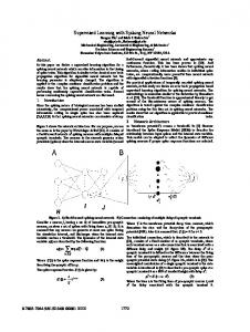
of neurons, we can classify ANNs into different generations. In 1943, McCulloh and Pits formulated the first artificial neuron, famously termed McCulloh-Pits neuron. In it, the neuron is modeled using thresholding function as the activation function. The thresholding is performed on the weighted sum of inputs as non-linear operation. This constitutes the first generation of ANNs [1]. The examples of first generation ANNs that use McCulloh-Pits neurons are Rosenblatt’s Perceptron, Hopfield nets, Bidirectional Associative Memory, Boltzman machines etc. and are capable of outputting binary outputs only. Theoretically, these neural networks with hidden layer are capable of approximating any Boolean function. In the second generation of ANNs [1], the neuron is modeled using monotonicallyincreasing continuous piecewise differentiable activation function which is able to process inputs and respond with real-valued outputs. Sigmoid function, hyperbolic tangent function, piecewise linear function, Gaussian function, Chebyshev polynomial etc. are some examples of activation functions used in ANNs of the second generation. The second generation of ANNs are very powerful, in the sense that they can approximate any real valued function to arbitrary precision within a given interval as stated by universal approximation theorem [3,4]. They have also proven their computational prowess through various practical applications and are the current state of the art in machine learning. The examples include Multilayer Perceptron (MLP), Radial Basis Functions (RBF), Self Organizing Maps (SOM), Elman Networks [5,6], convolutional neural networks [7], deep neural networks [8,9] etc. In the third generation of ANNs [1], the neuron is modeled using spiking neurons. Spiking neurons are mathematical model of biological neurons and similar to biological neurons, they process inputs in the form of a sequence of events in time, called spikes and produce output response in the form of spikes as well. This is drastically different from the real/binary input output values of the first and second generation of ANNs, however, it is exactly the way in which biological neurons exchange information between them. A Spiking Neural Network (SNN) is an ANN that uses spiking neurons as its computational units. It is less abstract than the ANNs of first and second generation and has increased similarity to the biological network. We will introduce details of SNN in the following section, followed by motivation behind SNNs. We will then clearly list the objectives of this thesis and out major
Nanyang Technological University
Singapore
Ch. 1. Introduction 1.1. Spiking Neural Networks
Page : 3
contributions. Finally we will end this chapter with an overview of the contents of this thesis.
1.1
Spiking Neural Networks
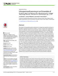
Spiking Neural Networks are ANNs that have spiking neurons as their computational units. Spiking neurons differ from non-linear activation function used in earlier generation of ANNs in the sense that they exchange information in the form of spikes rather than numeric input-output. The question arises, what are spikes exactly? We have plotted the activity in a visual cortex neuron in figure 1.1. 40
u[mV]
20 0 −20 −40 −60
0
0.2
0.4
0.6
0.8
1
1.2
1.4
1.6
1.8
2
t[s]
Figure 1.1: In vivo membrane potential of visual cortex neuron.1 The plot shows the readings of the electric potential of the neuron, termed membrane potenital, over time. We can see that at different instances, the membrane potential suddenly jump by around 100 mV. These jumps are typically of 1-2 ms duration and the pulse event is called spike. The nature of spike potential is not important, rather the number of spikes and the time of spikes is important [10]. In SNNs, the inputs to the ANN is spikes and the output is also spikes i.e. the currency of information exchange in SNN is in terms of spikes. This is illustrated in figure 1.2. Computation in terms of spikes means the information is encoded with respect to time. This brings an additional dimension of time as means of information exchange. Further, the inherent delay in the synapse and the time constant of a spiking neuron response (cf. Chapter 2.2.4) provides a memory feature in built in SNN and the recurrence due to refractory response of a spiking neuron bestows SNN with recurrent structure without really going through the complexity of recurrent neural networks. This makes SNNs potentially very useful, especially 1
Courtesy http://medicine.yale.edu/lab/mccormick/data/index.aspx
Nanyang Technological University
Singapore
Ch. 1. Introduction 1.1. Spiking Neural Networks
Page : 4
··· .. .
.. .
··· ···
Input Spikes
··· Spiking Neural Network
Output Spikes
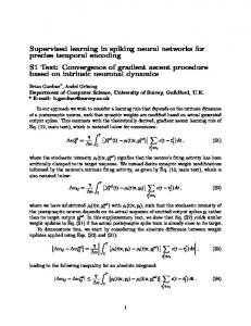
Figure 1.2: Computation in terms of spikes. The vertical lines in the input and output represent spikes. for the processes that are temporal, such as audio, video etc. The computation in terms of spike, however, adds complexity of encoding the real world numeric inputs into spikes to encode the information in time axis. For this, we need to employ special measures to encode the real world numeric inputs into spikes (cf. Chapter 2.3). We will now discuss the significance and usefulness of SNNs.
1.1.1
The Biological Inspiration
It has been known to researchers for a long time that the currency of information exchange in biological neurons is spikes. Since SNNs also process and transmit information in the form of spikes, they resemble the biological phenomenon closely, especially compared to the first and second generation of ANNs. The increased similarity to biological phenomenon makes SNNs very useful tool in modelling and analysis of biological neural system [11–15]. This, although not the sole motivation, is an inspiration towards computing in terms of spikes. We know for a fact that biological neurons exchange information in the form of spikes. The question “How exactly is the information encapsulated by a spike train?” still does not have clear answer. There are two school of thoughts on how the information is exchanged using spike train: rate encoding and pulse encoding. Classically, it was argued that the totality of the information being transmitted is contained by the firing rate of a neuron and the exact timing of spike does not matter. This principle is called rate encoding [1, 16–25]. The real numeric inputs and outputs of the first and second generation of neural networks are loosely interpreted as the instantaneous firing rate of the neurons in rate coding principle. However, numerous observations have been made in neuroscience, especially in the visual cortex and auditory neurons, where the neuron response over successive
Nanyang Technological University
Singapore
Ch. 1. Introduction 1.1. Spiking Neural Networks
Page : 5
layers is so swift that the firing rate interpretation is not plausible. The response is so quick that there is not enough spikes along subsequent layers to make an estimate of the firing rate. These findings suggest that the precise timing of spike carries significant amount of information being transmitted [1, 19–26]. The idea that precise time of spikes carry information is termed pulse encoding. Since few spikes can transmit useful information, SNNs can potentially process the information in efficient and rapid manner which makes SNNs an appealing prospect as efficient computational unit.
1.1.2
Significance of SNN as a Computational Unit
During the early years of research on SNN as a computational unit, Wolfgang Maass conducted several theoretical analysis on the complexity of computing with spiking neuron. For his analysis, he mostly considered simple abstract spiking neurons, namely Type A and Type B neurons [1, 20, 21, 27] (cf.Chapter 2.2.5). Table 1.1: Computational capacity of SNN with Type A neuron on Boolean functions Boolean function
No of hidden layer neurons required SNN† Threshold circuit MLP
Coincidence Detection: {0, 1}2n → {0, 1} ( 1 if ∃i : xi = yi CDn (x, y) = 0 otherwise
†
Element Distinctness: (R+ )n → {0, 1} 1 if ∃(i 6= j) : xi = xj EDn (x) = 0 if ∀(i 6= j) : |xi − xj | ≥ 1 arbitrary otherwise No hidden layer in SNN.
�
n log(n+1)
�
1
Ω
1
Ω(n log(n))
1
Ω(n /2 )
at least
n−4 2
−1
Table 1.1 summarizes the theoretical results on computational capacity of SNNs on Boolean function deduced by Wolfgang Maass [1]. We can see that a single SNN can achieve the Boolean results on CDn and EDn Boolean functions whereas for threshold based neural network and MLP, we require an ANN with multiple hidden neurons. The functions CDn and EDn serve as example Boolean functions to illustrate the usefulness of SNN. In addition, we have the following theoretical result as well: Any threshold circuit of s gates having real valued inputs from [0, 1]n can be simulated by a network of O(s) spiking neurons of Type B. [1](pp. 1668)
Nanyang Technological University
Singapore
Ch. 1. Introduction 1.2. Main Contribution
Page : 6
Since, a threshold circuit with hidden layer can approximate any Boolean function, it follows that SNNs can also approximate any Boolean function. Michael Schmitt [28] extended the theoretical results of Wolfgang Maass further showing the usefulness of SNNs in computing Boolean functions. In [27], Wolfgang Maass theoretically studied noisy spiking neuron (similar to Spike Response Model. cf. Chapter 2.2.4) with stochastic spiking. He proved the following result: For any given �, δ > 0 one can simulate any given feedforward sigmoidal neural net N with activation fucntion π by a network NN,�,δ of noisy spiking neurons in temporal coding. [27](pp. 213) This in conjugation with universal approximation theorem [3,4] means that SNNs are unviersal approximators. These theoretical results suggest open whole world of possibilities for SNN as a computational unit. The realization of these theoretical potential is, however, in its infancy [17]. Nevertheless, aforementioned theoretical potential renders SNNs a compelling research topic.
1.1.3
Neuromorphic Significance
Recently, the research in the field of hardware based neural networks has grained much traction, with the focus on implementing brain-like spike based computation in dedicated hardware [29–33]. These chips are called neuromoprhic circuits. Some of the currently popular advanced neuromorphic chips include IBM True North [29], SpiNNaker [31, 34] etc. Apart from studying neuron behaviour and simulating brain functions, these chips are extremely low power devices. Neuromorphic are extremely efficient in terms of chip area savings and energy savings compared to conventional CPUs and GPUs based machine learning networks [35–37]. These developments in neuromorphic chips makes learning using SNN a very exciting field.
1.2
Main Contribution
Although SNNs differ from first and second generation of ANNs in the way in which neuron is modeled, the inherent non-linearity and dynamic nature of a spiking neuron means that we cannot directly tap into the broad range of algorithms
Nanyang Technological University
Singapore
Ch. 1. Introduction 1.2. Main Contribution
Page : 7
that have been developed for first and especially second generation of ANNs. A handful of methods, both supervised and unsupervised, have been developed for training an SNN. We will discuss in detail about these methods in detail in Chapter 3. As far as learning in a multilayer framework using SNN, we are left with SpikeProp [2] and its derivatives and Multilayer extension of ReSuMe [38]. SpikeProp and its derivatives mostly react to the first spike of the neuron only and ignore the subsequent spikes. Therefore, the full potential of efficient information processing using spike train is mostly untapped. The complex non-linear dynamic behavior of spiking neuron means that stability and convergence issues are of significant importance, more so compared to MLP networks. It is highly desirable to have learning methods that exhibit stable and convergent nature. Since simulating an SNN on a traditional sequential machine is a time consuming process, the assurance of stability and convergence is an important trait to have. In addition faster learning is also immensely valuable. Stability, convergence and faster learning is even more significant asset for leaning methods dedicated to multiple spiking SNN. The aim of this thesis is to design and develop fast, stable and convergent methods to learn in an SNN with multilayer architecture, first for single spiking variant and extend the concept to achieve similar results for multiple spiking SNN as well. The main contributions of this thesis are summarizes as follows. 1. An adaptive learning rate rule for SpikeProp based on weight convergence criterion (SpikePropAd) is proposed [39,40]. The algorithm reinforces SpikeProp learning with weight convergence based on Lyapunov criterion and the adaptive learning rate is determined based on the weight convergence criterion. The weight convergence results ensures more successful learning instances and the adaptive learning rate means that the learning is substantially faster than the original SpikeProp method. 2. An adaptive learning rate rule for delay learning extension of SpikeProp based on delay convergence criterion (SpikePropAdDel) is proposed [41]. The delay convergence is based on Lyapunov criterion and the adaptive delay learning rate is deduced from the delay convergence condition. The adaptive learning rate for weight from SpikePropAd and the adaptive learning rate for delay constitute SpikePropAdDel. The weight and delay convergence means that there is more success in learning. Since we can tune delay as well, the learning is faster compared to learning weights only using SpikePropAd and
Nanyang Technological University
Singapore
Page : 8
Ch. 1. Introduction 1.3. Other Current Research in SNN a lot faster than plain SpikeProp.
3. We use conic sector stability theory along with Lyapunov convergence to develop robust stability and convergence criterion for SpikeProp. This analysis ensures stability and convergence of learning method even in presence of external disturbance. We also employ function based adaptive learning rule and individual error analysis to develop SpikePropR algorithm [42]. Along with that, a dead-zone adaptive learning rule based on total network error is introduced – SpikePropRT algorithm [43]. Both methods are robust to noise and show excellent convergence performance and good speed as well. SpikePropRT is slightly better overall. 4. We develop a new weight update strategy suitable for learning a spike train in continuous manner – EvSpikeProp [44, 45]. We also perform weight convergence and robust stability analysis on EvSpikeProp and based on stability and convergence criterion, introduce a dead-zone adaptive learning rule – EvSpikePropR [44]. We demonstrate better convergence and higher success rate in learning using EvSpikeProp along with excellent speed of learning as well.
1.3
Other Current Research in SNN
Apart from computational unit, the research in SNN are mostly in neuroscience in trying to understand and interface biological neurons. They are of great importance in neuroscience as a useful tool to model brain functionality. There have been high profile efforts to use SNN to simulate brain network, viz. The Blue Brain project [11]. SNNs have also been used to understand the working of small scale natural system such as a cricket neural system [14]. Other research area in SNN include memory models [12, 13], neuroprosthetics and brain machine interface [46, 47] etc. Usually, simulating an SNN requires tremendous resources and time. Lately, there have been numerous effort for efficient simulation of spiking neural networks using CPU & GPU [11, 48–52] and special neuromorphic circuits as well [29, 30, 53].
Nanyang Technological University
Singapore
Ch. 1. Introduction 1.4. Overview of Thesis
1.4
Page : 9
Overview of Thesis
This thesis consists of nine chapters. The contents of this is organized as follows. In this Chapter, we have introduced SNN, the motivation behind research in SNN, our main contribution and current state of research in SNN. In Chaper 2, we will go through the basic definitions and fundamentals of spiking neuron. We will introduce various mathematical model of spiking neuron and discuss their advantages and disadvantages. We will also discuss about how the information is encoded in spikes and how the output spikes are interpreted. In Chapter 3, we will elaborate on existing learning methods for supervised learning in SNN, list their issues and advantages. Our focus will be on learning methods that can train an SNN with hidden layer and we will describe those learning methods in detail. In Chapter 4, we will explain the fundamentals of non-linear stability theory and some key concepts that we will make use of later in the thesis. We will first discuss key mathematical ideas before we explain the stability methods. Our focus in Chapter 4 will be on Lyapunov stability and conic sector stability. In Chapter 5, we will introduce adaptive learning rate algorithm, SpikePropAd, as an extension of SpikeProp. The adaptive learning rate is based on weight convergence analysis of SpikeProp and guarantees convergence in terms of weight parameter. In Chapter 6 we continue on the same concept for adaptive learning rate for delay learning, SpikePropAdDel, this time using delay convergence analysis of delay learning extension of SpikeProp. In Chapter 7, we will derive robust stability results along with convergence condition based on total error and individual error: SpikePropRT and SpikePropR learning algorithms. The robust stability means that the learning process is stable even in presence of external disturbance and weight convergence means that learning converges in terms of weight parameter. In Chapter 8, we will formalize event based weight update rule, EvSpikeProp, for learning spike train. We will also perform convergence and stability analysis of EvSpikeProp to develop enhanced event based learning rule– EvSpikePropR – in Chapter 8.
Nanyang Technological University
Singapore
Page : 10
Ch. 1. Introduction 1.4. Overview of Thesis
Finally in Chapter 9, we will summarize this thesis and recommend future research directions.
Nanyang Technological University
Singapore
Chapter 2 Spiking Neuron Basics Your brain is built of cells called neurons and glia – hundred and billions of them.
Each one of
these cells is as complicated as a city. —David Eagleman, 2012
The main component that differentiates a Spiking Neural Network from the previous generation of Artificial Neural Networks is the computational unit, which is a spiking neuron rather than some functional unit governed by activation function. Formally, a Spiking Neural Network is defined as: Spiking Neural Network — A Spiking Neural Network is a massively parallel distributed system made up of individual computational units comprising of spiking neurons which processes its inputs in the form of spike event and responds with spike event. The knowledge is stored in the synaptic weights and synaptic delays of the interneuron connection and is acquired by the network from its environment through a learning process. and a spiking neuron is defined as: Spiking Neuron — A spiking neuron is a mathematical model that describes the dynamics of a biological neuron, its response to incoming spike events through different synapses and is able to describe spike events, either directly or indirectly. In this chapter, we will discuss different mathematical models of a biological neu11
Page : 12
Ch. 2. Spiking Neuron Basics 2.1. Dynamics of a Biological Neuron
rons that can be used as the computational unit in the form of spiking neuron in an SNN. The mathematical models of neuron are the product of researches in Computational Neuroscience pertaining to electrophysiological behaviour of a neuron. In this chapter, we will discuss the dynamics of a biological neuron. Next, we will discuss about different spiking neuron models with focus on their biological plausibility as well as their ease of implementation in large scale. A spiking neuron responds to a spike and reacts with a spike event. However, the real word signals are numeric valued. We will discuss different school of thoughts about the numeric interpretation of spikes and how real world data can be represented in terms of spikes.
2.1
Dynamics of a Biological Neuron
We can see the plot of electrophysiological reading of a visual cortex neuron in figure 1.1. The voltage value of the neuron is called membrane potential, usually denoted by u(t), and the distinct short surges in membrane potential occurring from time to time are the spikes. Before we proceed to describe the dynamics of a biological neuron, we will define some formal terms: Spike or Action Potential — A spike or an action potential is a brief electric pulse in membrane potential, typically 1 to 2 ms in duration and an amplitude of about 100 mv which roughly look alike and is usually followed by a dip in membrane potential, that occurs in regular or irregular intervals. The action potential is the elementary unit of signal transmission [10]. Spike Train — A chain of action potentials emitted by a single neuron is called a spike train – a sequence of stereotyped events which occur at regular or irregular interval [10]. Synapse — The site where the axon of a presynaptic neuron makes contact with the dendrite (or soma) of a postsynaptic neuron cell is the synapse [10]. In the event of spike at a presynaptic neuron, synapse release neurotransmitters from the presynaptic terminal into the synaptic cleft which creates an imbalance in ionic concentration. The imbalance in ionic concentration effects the membrane potential of postsynaptic neuron such that the postsynaptic neuron is more likely
Nanyang Technological University
Singapore
Ch. 2. Spiking Neuron Basics 2.1. Dynamics of a Biological Neuron
Page : 13
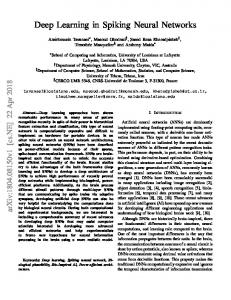
to emit a spike or less likely to emit a spike depending upon whether the synapse is excitatory synapse or inhibitory synapse [10,25]. The resulting effect of an input spike on postsynaptic neuron is called Post-Synaptic Potential (PSP). The PSP via excitatory synapse is called Excitatory Post-Synaptic Potential (EPSP) which typically increases the membrane potential above its resting potential, usually denoted by urest . The resting potential in biological neurons is typically around -70 mV. We can alternatively measure the membrane potential with reference to resting potential as well and consider 0 mV as resting potential. Similarly, the PSP via inhibitory synapse is called Inhibitory Post-Synaptic Potential (IPSP) which decreases the membrane potential below resting potential. A typical EPSP and IPSP response of a biological neuron is shown in figure 2.1. The magnitude of PSP depends on the synaptic weight or synaptic efficacy and the immediacy of PSP after spike is determined by synaptic delay which is dependent on the length of the synapse that the spike needs to travel. The cumulative effect of all the PSPs from presynaptic neuron forms the pre-spike membrane potential. u(t) EPSP ε(t − s)
u(t)
s
s
t
ε(t − s)
t
IPSP
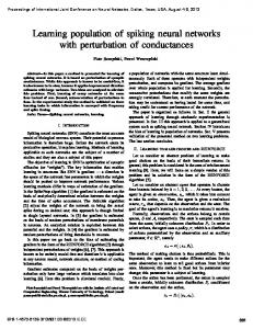
Figure 2.1: Typical EPSP and IPSP response of a biological neuron. When the pre-spike membrane potential increases from resting potential high enough, usually called threshold value, the linear accumulation of PSP breaks down and it exhibits a pulse like excursion, called spike or Action Potential (AP) [10]. After spike, the neuron membrane potential does not return to resting potential. Instead, the membrane potential passes through a phase of hyperpolarization below the resting value. This hyperpolarization is called After-Hyperpolarization Potential (AHP). The AHP is due to what is called refractory response of the neuron. There is a certain amount of time immediately after the action potential when the neuron is unable to fire at any cost. This period is called absolute refractory period. After absolute refractory period, the neuron still hesitates to fire, but is able to fire if the cumulative PSP is high enough. This phase is known
Nanyang Technological University
Singapore
Ch. 2. Spiking Neuron Basics 2.2. Models of Spiking Neuron
Page : 14
as relative refractory period. This behavior of a biological neuron is depicted in figure 2.2. u(t)[mV]
Spike (AP)
20
5 −20
10
15
−80
t[ms]
EPSPs urest IPSP
−100 −120
25
ϑ
−40 −60
20
AHP synaptic efficacy refractory response
−140 −160
input spikes
t
Figure 2.2: Dynamics of a biological neuron.
2.2
Models of Spiking Neuron
A spiking neuron tries to describe the dynamic behavior of a biological neuron mathematically with varying degree of detail. We will discuss different mathematical models suitable for this purpose next.
2.2.1
Hodgkin-Huxley Model
Alan L Hodgkin and Andrew F Huxley made a detailed study of action potential in Squid Giant axon and based on their ionic conduction model, they came up with what is now famously known as Hodgkin-Huxley model of neuron. They described the ionic conduction channel with various effective conductance model for Sodium and Potassium ion channel with each of the variable conductance separately modeled via their own set of non-linear differential relation. The electrical
Nanyang Technological University
Singapore
Ch. 2. Spiking Neuron Basics 2.2. Models of Spiking Neuron
Page : 15
model that Hodgkin-Huxley proposed for modeling the Squid Giant axon is illustrated in figure 2.3. Input Current I(t)
gleak
K
Na u(t)
C Eleak
EK
ENa
Figure 2.3: Hodgkin Huxley model based on ion channels. The membrane potential, u(t), is described using following set of equations [54]: C
du = −gNa m3 h (u − ENa ) − gK n4 (u − EK ) − gleak (u − Eleak ) + I(t) dt (2.1a) dm m − m0 (u) =− dt τm (u) h − h0 (u) dh =− dt τh (u) dn n − n0 (u) =− dt τn (u)
(2.1b) (2.1c) (2.1d)
where C is capacitance of the membrane gNa , gK and gleak are the conductance parameters for different ion channels ENa , EK and Eleak are the equilibrium potentials of ion channels m, n and h describe the opening and closing of voltage dependent channels I(t) is the injection current For more complex neurons with additional ion channels, one can simply include additional conductance term for it in (2.1). With suitable model for conductance parameters and channel gate functions, Hodgkin-Huxley model provides very realistic results. It is for their remarkable modeling of physiological behavior of
Nanyang Technological University
Singapore
Ch. 2. Spiking Neuron Basics 2.2. Models of Spiking Neuron
Page : 16
neuron, Hodgkin and Huxley were awarded Nobel Prize in Physiology or Medicine in 1963.
Despite being very accurate model of a neuron, the different non-linear dynamic interrelationship in the coupled system of differential equation makes it very difficult to efficiently solve the system of differential equation, especially when it comes to solving it for a large network of neurons interacting with each other. Therefore, Hodgkin-Huxley model is not suitable in modeling a population of spiking neurons.
2.2.2
Two Dimensional Neuron Model
The complexity of Hodgkin-Huxley model can be simplified for practical purposes exploiting the similarities between ionic conductance parameters and using the idea of separation of time scale. These simplification reduce the complex formulation of Hodgkin-Huxley model into a system of two differential equations which can be generalized into following form [10]. C
du = f (u, w) + I(t) dt dw = g(u, w) dt
(2.2a) (2.2b)
Where, w(t) is the membrane recovery variable.
There are a handful two dimensional model of neuron, each with diverse origin. However, they follow the same system of equation described in (2.2). Some of the two dimensional models are listed below:
Nanyang Technological University
Singapore
Ch. 2. Spiking Neuron Basics 2.2. Models of Spiking Neuron
Page : 17
u3 −w , C=1 3 g(u, w) = 0.08(u + 0.7 − 0.8 w)
FitzHugh-Nagumo model [55]
f (u, w) = u −
Morris Lecar model [56]
f (u, w) = −gCa Mss (u) (u − ECa ) − gK w (u − EK ) − gL (u − EL ) Wss (u) − w g(u, w) = Tw (u)
Izhikevich Model [57]
f (u, w) = 0.04 u2 + 5 u + 140 − w
, C=1
g(u, w) = a (b u − w) spike if u ≥ 30 mV, then
u ← c w ← w + d �
AdEx Adaptive exponential integrate-and-fire model [58]
f (u, w) = −gL (u − EL ) + gL ∆T exp
u−ϑ ∆T
� −w
a (u − EL ) − w τw u ← u rest spike if u ≥ ϑ, then w ← w + d
g(u, w) =
These two dimensional model of neuron are simple enough to be practically implement for a population of spiking neurons and are able to exhibit complex dynamic behavior seen in biological neurons.
2.2.3
One Dimensional Neuron Model
For even more scalable simulation, the two dimensional model of neuron can be further simplified into single differential equation. This is called one dimensional neuron model which takes the following general form: du = f (u) + R I(t) dt spike if u = ϑ, then reset u ← urest τ
(2.3)
The function f can take different form resulting in Leaky Integrate and Fire (LIF) as linear formulation and Nonlinear Integrate Fire model. They are listed below:
Nanyang Technological University
Singapore
Ch. 2. Spiking Neuron Basics 2.2. Models of Spiking Neuron
Page : 18
Leaky Integrate and Fire (LIF) [4, 10, 25]
f (u) = −(u − urest )
Exponential Integrate and Fire (EIF) [59]
) f (u) = −(u − urest ) + ∆ exp( u−ϑ ∆
Quadratic Integrate and Fire (QIF) [10]
f (u) = c2 (u − c1 )2 + c0
These one dimensional model of neuron are very simple and easy to implement, however, their major drawback is that these model do not demonstrate the refractory behavior of neuron which is a major neuronal behavior. Nevertheless, they are reliable in predicting the response spike to input spikes barring very nuanced behavior [60].
2.2.4
Spike Response Model
The previous models of neuron were based on modeling the membrane dynamics of biological neuron. Spike Response Model (SRM) on the other hand is based on characterization of behavior observed in biological neuron. It was introduced by Gerstner [61]. This model of neuron is based on linear filters corresponding to PSP, refractory response and injection current. Consider a neuron N´ which is receiving input spikes from a set of presynaptic ´ Denote the set of delayed neurons Γ´ = {´ı : N´ı is presynaptic to N´} = I. synaptic connection by K the synaptic weight of k th synapse, where k ∈ K, from (k) N´ı to N´ by w´´ı , the synaptic delay of k th synapse, where k ∈ K, from N´ı to N´ by (k) (1) (2) (f −1) d´´ı , the set of previous firing times of neuron N´ by F´ = {t´ , t´ , · · · , t´ } and the injection current input to neuron N´ by I(t). Then the pre-spike membrane potential is modeled as: delayed post synaptic response
refractory response
u´(t) =
z X
(f −1)
t´
}| { zX X X }| { (k) (f ) (f −1) (k) ν(t − t´ )+ w´´ı ε(t − t´ı − d´´ı )
∈F´
´ı∈Γ´ t(f ) ∈F ´ ı
´ ı
k
(2.4) injection current response
z Z +
∞
}|
{
κ(r) I(t − r) dr
0
where ν(s) is the refractory response kernel which models potential reset after spike, ε(s) is the spike response kernel which models normalized PSP and κ(s) is the injection current kernel which models the response to injection input current
Nanyang Technological University
Singapore
Ch. 2. Spiking Neuron Basics 2.2. Models of Spiking Neuron
Page : 19
[25, 62]. The commonly used SRM kernels are (see [2, 25, 61, 63, 64]):
ν(s) =
−ϑ e− τsr Θ(s) abs − s−δ τr
−ν e 0
OR
Θ(s − δ abs ) − K Θ(s) Θ(δ abs − s)
s e− τs Θ(s) s e− τss Θ(s) ε(s) = τs s 1− τss e Θ(s) τ s s s (e− τm − e− τs )Θ(s),
OR OR OR 0 ≤ τs ≤ τm
s
κ(s) = e− τc Θ(s) where Θ(·) is the Heaviside step function and τ is the time constant corresponding to the kernels. Different form of spike response kernel, ε(s), is possible for excitatory and inhibitory synapse. It is common to represent inhibitory synapse by negative weight and use the same spike response kernel. When the membrane potential rises up to a threshold value ϑ, N´ emits a spike at (f ) t = t´ i.e. (f )
t´
(f )
(f )
(f )
(f −1)
: u´(t´ ) = ϑ, u0´(t´ ) > 0, t´ > t´
(2.5)
SRM model of neuron, although seems simple, is quite general. With proper response kernels, it can simulate very complex neuronal behavior observed in biological neurons [10, 25]. In addition, this neuron model is rather straightforward to implement as well. Denote the input spikes from neuron Ni in vector form as ti . The sum of normalized PSP response from neuron N´ı is usually denoted as (k)
y´´ı (t, ti ) =
X
(f )
(k)
ε(t − t´ı − d´´ı )
(2.6)
(f ) t´ı ∈F´ı
Denote the set of all the weights of N´ by ´
w´I´ = [· · · , w´´ı , · · · ]T ∈ R|I ||K| (k)
Nanyang Technological University
(2.7)
Singapore
Ch. 2. Spiking Neuron Basics 2.2. Models of Spiking Neuron
Page : 20
and the corresponding spike response vector by ´
y ´I´(t, ti ) = [· · · , y´´ı (t, ti ), · · · ]T ∈ R|I ||K| (k)
(2.8)
Then the Spike Response Model can be succinctly written as u´(t) =
X
ν(t −
(f −1) t´ )
+
wT´I´y ´I´(t, tI´)
Z +
(f )
(f )
(f )
(f )
κ(r) I(t − r) dr
(2.9)
0
(f −1) t´ ∈F´
t´
∞
(f −1)
: u´(t´ ) = ϑ, u0´(t´ ) > 0, t´ > t´
Usually, the refractory response kernel, ν(s), and the spike response kernel, ε(s), die out with time. The refractory response of the most recent neuron spike, de(f −1) noted by t´ , is the dominant refractory kernel. Further, the effect of any input spike before the last neuron spike is also insignificant. Therefore, we can reduce the set of input spikes from presynaptic neuron by including additional restriction as follows. (f )
F´ı = {t´ı
(f )
(f −1)
(k)
: ´ı ∈ Γ´ & t´ı + d´´ı > t´
}
(2.10)
This results in short term memory variant of SRM, called Short-term Memory neuron [25]. (f −1)
u´(t) = ν(t − t´ (f )
t´
(f )
) + wT´I´y ´I´(t, tI´) (f )
(f )
(2.11) (f −1)
: u´(t´ ) = ϑ, u0´(t´ ) > 0, t´ > t´
Further, if we consider only the first spike of the neuron, the refractory response is vestigial. This is called SRM0 model [2, 25]. u´(t) = wT´I´y ´I´(t) (f )
t´
2.2.5
(f )
(2.12) (f )
: u´(t´ ) = ϑ, u0´(t´ ) > 0
Type A and Type B Spiking Neuron
For the study of computational capacity of spiking neurons, Wolfgang Maass [1] used spiking neuron model with simplified spike response function and variable
Nanyang Technological University
Singapore
Ch. 2. Spiking Neuron Basics 2.3. Spike Coding
Page : 21
threshold to represent refractoriness. Mathematically, they are defined as follows. u´(t) =
X
(f )
w´´ı ε(t − t´ı − d´´ı )
(2.13)
´ı∈Γ´ (f )
t´
(f −1)
(f )
: u´(t´ ) = θ(t − t´
)
Type A and Type B spiking neuron differ in their spike response function. The former has simple pulse function as spike response function and the latter has triangular function as spike response function. This is depicted in figure 2.4. Type A ε(t − s)
u(t) 1
1 t
s (a)
∞
Type B (f ) θ(t − t´ ) ε(t − s) ϑ
u(t)
t
s (b)
t
(f )
t´
(c)
Figure 2.4: Type A and Type B spiking neurons as defined in [1] (a) spike response function for Type A spiking neuron (b) spike response function for Type B spiking neuron (c) variable threshold for refractoriness. These simple models of spiking neuron have been used to show various computational prowess of spiking neural network (cf. Chapter1.1.2).
2.3
Spike Coding
The currency of information exchange in an SNN is spike. On the other hand, the real world signals and data are numeric values. To use an SNN as a computational unit, it is of paramount importance to convert the real world signals into spikes and back. It is clear that spike train carry information between neurons. However, what aspect of spike train is exactly responsible for information transfer is not very clear. There are two schools of thought: rate encoding and pulse encoding (cf. Chapter 1.1.1). Rate encoding assumes that the information is borne by the firing rate of the spike train, whereas pulse encoding advocates that precise timing of each individual spike carries information. For interpretation of output spikes, winner-takes-all scheme for classification i.e. whichever neuron fires first is the associated class or classification based on more
Nanyang Technological University
Singapore
Ch. 2. Spiking Neuron Basics 2.3. Spike Coding
Page : 22
active neuron i.e. whichever neuron shows more spike activity is the associated class are plausible methods of interpreting output spikes. As far as encoding numeric signals into spikes, traditional method in neuroscience is to consider spikes as a Poisson process with instantaneous firing rate modulated by input signal [16]. A Linear Non-Linear Poisson (LNP) model based on analysis of LIF and EIF neuron model produces better spike encoding compared to Poisson encoding [65]. Even more accurate spike generation has been proposed by Pillow et al. using spiking neuron model: generalized integrate and fire model [66] and Generalized Linear Model (GLM) [67]. For computational purposes, in case of binary inputs the signal can be encoded using earlier or later spike. The real inputs on the other hand need special treatment. A simple method is to use interspike interval to represent the numeric data. The methods described above that are used in neuroscience are also suitable for encoding numeric data. Other methods include Threshold-based encoding (TBE) [68,69], adaptive response method [70] which encode numeric time series into spike trains. However, these methods produce a spike train. The issue is that most of the methods for learning in multilayer spiking neural network cannot handle multiple spikes. Population encoding [2] is an effective method for encoding numeric signal values into single spike time for a group of neurons. Population encoding and Threshold based encoding are described below.
2.3.1
Population Encoding
In population encoding, an array of Gaussian receptive fields that are uniformly separated with overlapping profile along the input data range is used to represent input neurons. Different input value have different strength of response in the receptive fields. If the strength of response is high for a neuron’s receptive field, earlier spike is encoded for it and if the strength of response is low for a neuron’s receptive field, later spike is encoded for it. If the strength of response is very low, no spike is encoded for the corresponding neuron [2]. The spike times are rounded to nearest time unit. In figure 2.5, the process of population encoding is demonstrated using four Gaussian receptive fields to encode the input numeric into spikes from time t = 0 to 4 units.
Nanyang Technological University
Singapore
Ch. 2. Spiking Neuron Basics 2.3. Spike Coding
Page : 23
Input range
t(f )
1
0
0.882 0.606
1
0.044
2
⇒ 0.606 0.882
3 4
0.135 0 0.044 Imin
0.135 t(f ) = 0 1 2 3 4
Iin Imax
Figure 2.5: Population encoding of input values using Gaussian receptive fields. Bohte et al. [2] suggest distributing the center of Gaussian receptive fields at µi = Imin +
2 i − 3 Imax − Imin , 2 m−2
i = 1, 2, · · · , m
(2.14)
and their spread defined by σ=
1 Imax − Imin β m−2
(2.15)
where β controls the amount of spread, the input numeric is bounded by the range [Imin , Imax ]. The popualtion encoding scheme work similar to the Retinal Ganglion Cell (RGC) in eye and produces sparse encoding [2].
2.3.2
Threshold Based Encoding
Threshold based encoding (TBE), in contrast to population encoding, encodes the information in a continuous signal into on and off spikes rather than encoding the information over a population of neurons. In its basic form, a threshold is set in log-scale i.e. the threshold value changes by an order of magnitude. Whenever the change in input data exceeds the threshold, a spike is generated. If the change is increasing, an on spike is generated and if the change is decreasing, an off spike is generated. This process is depicted in figure 2.6. The green signal follows the input signal until it crosses threshold. Whenever it crosses the threshold, the signal reference is reset and an on or off spike is generated.
Nanyang Technological University
Singapore
Ch. 2. Spiking Neuron Basics 2.3. Spike Coding
Page : 24
input
on spike bC bC bC bC bC bC
bC bC bC bC bC bC bC bC bC
bC bC bC bC bC bC bC bC
bC bC
bC
bC bC bC
bC
bC bC bC
bC bC bC
bC bC bC bC bC
bC bC bC bC bC bC bC bC bC bC bC bC
off spike
time
log magnitude
log magnitude
input
reconstruction
time
Figure 2.6: Threshold based encoding of a continuous signal. This simple mechanism is able to track the changes in input signal quite well, Although it cannot track the finer nuances in the input, the overall changes is represented quite well. Therefore, it suits quite well to convert temporal signals into spike using TBE. In fact same principle is used to encode real signal into spikes in Silicon Retina [71] and Silicon Cochlea [72, 73] which produce the sensor readings directly in terms of spikes.
Nanyang Technological University
Singapore
Chapter 3 Supervised Learning in SNN: An Overview Networks of noisy spiking neurons with temporal coding have have a strictly larger computational power than a sigmoidal neuron with same number of units —Wolfgang Maass, 2000
There are abundant learning algorithms to train an MLP. One might think that we can port the learning algorithms for MLP in the realm of SNN and use them for SNN training with little or no modification. However, since spiking neurons have far more complex dynamics than continuously differentiable monotonically increasing activation function, we face a major hurdle while trying to take derivative of input-output functional of a spiking neuron. Almost all the learning algorithms for learning an MLPs requires the use of derivative, therefore, formulating the derivative of input-output functional of a spiking neuron is necessary to be able to use backpropagation based learning rules in context of SNNs. The inherent discontinuity in membrane potential and an added aspect of time into the mix pose additional challenges in learning using SNNs. There have been workarounds that circumvent the issues posed by SNNs and put forth a couple of learning algorithms specially tailored for SNNs. In spite of that, learning in SNNs is still a developing area [74]. Some learning methods have been extended from the domain of MLPs while some have been specifically developed for SNNs which utilize the salient features of spiking neurons and arrive at novel learning methods in SNNs [25]. 25
Page : 26
Ch. 3. Supervised Learning in SNN: An Overview
The unsupervised learning methods for SNNs are mostly variants of Hebbian Learning [25]. In neuroscience experiments, it has been observed that change in synaptic strength is a function of relative differences in input and output spike times [75, 76]. If the presynaptic spike precedes postsynaptic spike, in general the synaptic strength increases – potentation and if the postsynaptic spike precedes presynaptic spike, in general the synaptic strength decreases – depression. This phenomenon is called Spike Timing Dependent Plasticity (STDP) in neuroscience. STDP is the basis of Hebbian learning in SNN. Sometimes, the reverse behaviour to STDP takes place. This is called anti-STDP or anti-Hebbian plasticity [77]. Hebbian learning based unsupervised learning methods for SNN include Multilayer RBF for SNNs by Bohte et al. [63] and SOM for SNN by Ruf et al. [22]. Gerstner et al. [12] and Zamani et al. [13] use associative memory consisting of spiking neurons which act as unsupervised learning unit for SNNs. The supervised learning for SNNs can be categorized into various groups. We will describe them along with their pros and cons below. The first group of supervised learning method are the methods that train a single spiking neuron to learn a spike train. The methods include Remote Supervised Method (ReSuMe) [78,79], Chronotron [80], Spike Pattern Association Neuron (SPAN) [81,82], precise spike driven synaptic plasticity rule [83], Linear Algebraic Method [84] etc. These set of learning methods learn the weights parameter of a spiking neuron, given the set of input spike trains and output spike train. Some of these methods may also learn other parameters of a spiking neuron such as synaptic delay and firing threshold. These methods are usually independent of the spiking neuron model, which makes them versatile. These methods learn the parameters in batch mode, meaning complete set of input spike trains and desired output spike train need to be presented for learning. This makes them not well suited for learning in sequential fashion for indefinite time. Nevertheless, they can be used in mini-batch mode in such a scenario. Although, these learning methods learn weights for a single neuron, extension of ReSuMe called Multi-ReSuMe [38] has been forked to learn in a multilayer architecture as well. The next group of supervised learning method for SNNs fall into the category of reservoir computing methods. The methods include echo state network and liquid state machine [85–87]. Here, a pool of neurons with random interconnections between them is used. These neurons can even have self recurrence as well. The pool of neurons are referred to as reservoirs. The neurons in the reservoir receive spikes from input neurons. For output, a neuron randomly receives input from
Nanyang Technological University
Singapore
Ch. 3. Supervised Learning in SNN: An Overview
Page : 27
the reservoir neurons and its weight parameter is learned so that it emits output spike of desired characteristics. The output neuron is usually trained using one of the methods mentioned above i.e. SNN method for training a single neuron. As far as the reservoir is concerned, the neurons in this pool can also tune their weights using unsupervised STDP rule. The advantage of this method is that same reservoir network can be used to learn other patterns by simply adding an output neuron and connecting it to the reservoir neuron and continuous stream of spikes are handled naturally. Their major drawback, however, is that there is little control over how the reservoir is created as it is based on random connections and there is no general rule for designing a good reservoir. The recipe for creating a good reservoir is an acquired skill via experience and how they work is unclear. Next group of supervised learning methods for SNNs are the class of learning methods known as evolving Spiking Neural Networks (eSNN) [88]. The basic eSNN adds a neuron in the output layer on the fly for each new input pattern. The weights are determined by Rank Order (RO) coding, which uses the first input spike time to determine weight. The new neuron is merged to a pre-existing neuron if its acquired weight is similar to a pre-existing neuron, based on some similarity metric. When neurons are merged, their weights are averaged. This makes it vary fast learning method, requiring one pass only. However, the weight of a neuron does not change after that as a result it ignores the subsequent spikes at the input. The extensions to eSNN allow for adaptation of weights as a response to subsequent input spikes [89–92]. They differ on the manner in which weights are tuned for subsequent input spikes, for e.g., dynamic evolving Spiking Neural Network (deSNN) [89] uses Spike Driven Synaptic Plasticity (SDSP) rule whereas Basis Coupled Evolving Spiking Neural Network (BCESNN) uses basis coupled rank order learning to fine tune the weights. A special structured network of spiking neurons with spatially influenced connection between them has also been developed. It is called NeuCube [93]. The spatially arranged structure makes it suitable for spatial data. The NeuCube structure is similar to reservoir network in reservoir computing, with additional structural arrangement and no recurrence. In NeuCube, the output neuron is added using deSNN rule. It makes NeuCube suitable for spatio-temporal data. Another group of learning method for SNN are SpikeProp [2] and its derivatives viz. Extended SpikeProp [94], SpikeProp for multiple spiking neuron [17, 64, 95], Resilient Propagation (RProp) [96] etc. These methods allow learning in a multilayer architecture, similar to MLPs. Although, the presence of hidden layer gives
Nanyang Technological University
Singapore
Ch. 3. Supervised Learning in SNN: An Overview 3.1. Neural Network Architecture
Page : 28
them computational edge, their major drawback is that they are mostly limited to a single spike. In addition they also have issue of stability issues as well. Nevertheless, they are the among the very few SNN learning methods that can learn in a multilayer neural network architecture, making use of hidden layer. Among the supervised learning methods listed above, SpikeProp, its derivatives and Multilayer extension of ReSuMe [38] can deal with learning in an SNN with hidden layer. Reservoir computing methods do have hidden layer neurons, however, the learning takes place in output layer only. We will discuss these methods in detail in the following sections. But before that, we will formally describe the neuron architecture and speed-up techniques during forward simulation of SNN.
3.1
Neural Network Architecture
∂E ∂W IH
∂E ∂W OH
H (H)
N1
I (I) t1
(I) N1
.. .
.. . (I) ti
(O) t (O) 1 Σ N1 − ext �1 .
(O) t¯1
(O)
(O) t¯o
..
(H) Nh
(I) Ni
.. . (I) t|I|
(O) No
.. .
.. .
(I) N|I|
(O) N|O|
(H)
N|H| (1)
dhi
(2)
dhi (I)
(I) Ni
······
O
ti
(k)
dhi
to
− �ext o
Σ
(O)
t|O|
− �ext |O|
Σ
(O) t¯|O|
(1)
ε(·) ε(·)
ε(·) .. (|K|) . dhi ε(·)
whi
(2)
whi
(k)
whi
(H)
Nh
(H)
th
(|K|)
whi
Figure 3.1: SNN architecture with |K| delayed synaptic connections, |I| input layer neurons, |H| hidden layer neurons and |O| output layer neurons.
Nanyang Technological University
Singapore
Ch. 3. Supervised Learning in SNN: An Overview 3.1. Neural Network Architecture
Page : 29
In this thesis we will deal with three-layer-fully-connected feedforward neural network architecture. Each connection between two neurons consists of multiple delayed synaptic connections. Such a network is illustrated in figure 3.1. Here I, H and O denotes the set of input layer neurons, hidden layer neurons and output layer neurons. Furthermore, K denotes the set of delayed synaptic connection. Therefore, there are |I| input layer neurons, |H| hidden layer neurons, |O| output layer neurons and |K| delayed synaptic connections. (I)
(H)
Ni : i ∈ I denotes a neuron in input layer, Nh : h ∈ H denotes a neuron in (O) hidden layer and No : o ∈ O denotes a neuron in output layer. For the sake of brevity, we will denote a neuron in input layer, hidden layer and output layer by Ni , Nh and No respectively. We will refer to the detailed notation only when there is ambiguity in meaning. Similarly, the firing time of Ni , Nh and No is denoted (f ) (f ) (f ) by ti , th and to respectively. If we are only considering the first spike of the Ni , Nh and No , which is common in SpikeProp as we will see in Section 3.3, the first spike time is denoted by ti , th and to respectively. For k th : k ∈ K synaptic connection between Ni and Nh , synaptic weight is (k) (k) denoted by whi and synaptic delay is denoted by dhi . Similarly, for k th synaptic (k) connection between Nh and No , synaptic weight is denoted by woh and synaptic (k) delay is denoted by doh . All the weights associated with neuron Nh and No represented in vector form is defined as whI = [· · · , whi , · · · ]T ∈ R|I||K|
(k)
(3.1)
(k)
(3.2)
woH = [· · · , woh , · · · ]T ∈ R|H||K|
respectively and all the delays associated with neuron Nh and No represented in vector form is defined as (k)
(3.3)
(k)
(3.4)
dhI = [· · · , dhi , · · · ]T ∈ R|I||K| doH = [· · · , doh , · · · ]T ∈ R|H||K|
respectively. Next, the weight matrix associated with hidden layer neurons and output layer neurons represented in matrix form is defined as W HI = [· · · , whI , · · · ]T ∈ R|H|×|I||K|
(3.5)
W OH = [· · · , woH , · · · ]T ∈ R|O|×|H||K|
(3.6)
Nanyang Technological University
Singapore
Ch. 3. Supervised Learning in SNN: An Overview 3.2. Forward Simulation of SNN
Page : 30
respectively and the delay matrix associated with hidden layer neurons and output layer neurons represented in matrix form is defined as D HI = [· · · , dhI , · · · ]T ∈ R|H|×|I||K|
(3.7)
D OH = [· · · , doH , · · · ]T ∈ R|O|×|H||K|
(3.8)
respectively. These weights and delays hold the knowledge acquired by the SNN described in this thesis. Throughout this thesis, we use (¯·) notation to denote the ideal parameters. There(f ) fore, ideal spike value of output neuron is denoted by t¯o (t¯o if first spike is considered). Further, �ext o refers to the additive noise which acts as external disturbance to the system. This external disturbance is not additional disturbance that is added, but rather it is mixed with the desired spike firing time in learning sample, (f ) denoted by tˆo (tˆo if first spike is considered), which is always mixed with noise, i.e. ) ext ¯(f ) tˆ(f o = to + �o
tˆo = t¯o + �ext o
(3.9) (3.10)
We will use this additive model to perform detailed error analysis to prove stability of SNN learning algorithm later in Chapter 7 and Chapter 8. For the time being, one can ignore this disturbance term and continue.
3.2
Forward Simulation of SNN
Forward simulation is the first step during training a neural network. It is more important step for SNNs because it is the most taxing step during training process. This is because unlike traditional MLPs spiking neurons do not have closed form solution for their output spike times. As a result one must iteratively find the solution for output spike times of a spiking neuron which means that it requires multiple pass at different time to determine the solution. The general strategy is to perform a linear scan for say t = tstart : tres : tstop and keep on checking for the firing condition u´(t) > ϑ. There have been numerous efforts in efficiently simulating large scale spiking neural networks using CPUs and GPUs [11, 48–52]. This topic is out of the scope of this thesis. For our purposes, we use step-wise refinement technique on a progressively smaller interval to efficiently evaluate neuron spike
Nanyang Technological University
Singapore
Ch. 3. Supervised Learning in SNN: An Overview 3.2. Forward Simulation of SNN
Page : 31
time. This approach is described in Algorithm 1 for evaluating first spike time of a spiking neuron and in Algorithm 2 for evaluating spike train firing times of a spiking neuron. Algorithm 1 First firing time of Neuron N´ 1: 2: 3: 4: 5: 6: 7: 8: 9: 10: 11: 12: 13: 14: 15: 16: 17:
function CalcTfire(N´) tstep ← INIT_STEP t´ ← NO_FIRE repeat for t ← tstart : tstep : tstop do calculate u´(t) if u´(t) ≥ ϑ then t´ ← t tstart ← t − tstep tstop ← t break end if end for tstep ← tstep /STEP_FACTOR until tstep ≥ tres return t´ end function
. INIT_STEP = 1
. STEP_FACTOR = 10
Algorithm 2 Spike train firing times of Neuron N´ 1: 2: 3: 4: 5: 6: 7: 8: 9: 10: 11: 12: 13:
(f )
function CalcTfireMulti(N´, {t´ }, tstart , tstop , tstep ) if tstep < tres then (f ) (f ) {t´ } ← {t´ } ∪ {tstart } else for t ← tstart : tstep : tstop do calculate u´(t) if u´(t) ≥ ϑ then (f ) (f ) {t´ } ← CalcTfireMulti(N´, {t´ }, t − tstep , t, tstep /STEP_FACTOR) end if end for end if (f ) return {t´ } end function
This step-wise refinement method significantly speeds up forward simulation of SNN (appx. 50×), as it evaluates spike times in logarithmic order compared to linear order of plain brute force method.
Nanyang Technological University
Singapore
Ch. 3. Supervised Learning in SNN: An Overview 3.3. SpikeProp
Page : 32
3.3
SpikeProp
The SpikeProp algorithm for SNNs is the counterpart of the backpropagation algorithm for MLPs. It follows the principle of error sharing in hidden layer through gradient evaluation. As we mentioned before, the non-linear dynamic behavior of spiking neuron makes it difficult to evaluate derivative of spike event with respect to continuous time values such as membrane potential. Bohte et al. circumvent this issue in SpikeProp [2] by using linearization approximation of membrane potential in the neighborhood of neuron firing time. As it turns out, this so called approximation is mathematically correct which we will see shortly. Assumptions: 1. Each neuron in the network fires exactly once during the period under consideration. In other words, the neurons have long enough refractory period so that they are able to spike only once during the simulation interval. 2. The spiking neuron is modeled using Spike Response Model (SRM) (cf. Chapter 2.2.4) The assumption that a neuron fires exactly once allows us to greatly simplify the SRM model allowing us to get rid of refractory response and multiple input spike characterization. This results in what is known as SRM0 model. We will reiterate the SRM0 model again next. u´(t) = wT´I´y ´I´(t)
(3.11)
t´ : u´(t´) = ϑ, u0´(t´) > 0
Here, (k)
(k)
y´´ı (t) = ε(t − t´ı − d´´ı )
(3.12)
is the delayed spike response function (k)
y hI (tI ) = [· · · , yhi (ti ), · · · ]T ∈ R|I||K| y oH (tH ) = [· · ·
(k) , yoh (th ), · · · ]T
∈ R|H||K|
(3.13) (3.14)
are spike response vector for a neuron in hidden layer and output layer respectively
Nanyang Technological University
Singapore
Ch. 3. Supervised Learning in SNN: An Overview 3.3. SpikeProp
Page : 33
and Y HI (tI ) = [· · · , y hI´(tI ), · · · ]T ∈ R|H|×|I||K|
(3.15)
Y OH (tH ) = [· · · , y oH´ (tH ), · · · ]T ∈ R|O|×|H||K|
(3.16)
are spike response matrices of hidden layer and output layer respectively From (3.11), the membrane potential vectors are uH = [· · · , wThI y hI (tI ), · · · ]T = diag(W HI Y HI (tI )T ) ∈ R|H|
(3.17)
uO = [· · · , wToH y oH (tH ), · · · ]T = diag(W OH Y OH (tH )T ) ∈ R|O|
(3.18)
Even though, the mapping from membrane potential to spike time is an event mapping as defined in (3.11), for backpropagation, we need to transfer the error in spike time into error in membrane potential. For completeness, denote the functional that maps membrane potential in subthreshold regime into spike time as f (u´) = t´
(3.19)
and its corresponding vector function as f (u) = [f (u1 ), f (u2 ), · · · , f (un )]T : Rn → Rn
(3.20)
Then, one can write the operation in hidden layer framework as tH = f diag W HI Y HI (tI )T
��
= f d W HI Y HI (tI )T
�
(3.21)
where f d (·) = f (diag(·)) : Rn×n → Rn
(3.22)
Then, the input-output mapping of a single spiking SNN with one hidden layer can be written as � ��T � tO = f d W OH Y OH f d W HI Y HI (tI )T
(3.23)
Now, for SpikeProp rule, we proceed as follows. Since it is necessary to have u´(t´ ) = ϑ during spike event, taking differential with respect to weight on both
Nanyang Technological University
Singapore
Ch. 3. Supervised Learning in SNN: An Overview 3.3. SpikeProp
Page : 34
sides, we get du´(t´)
=0 (k) dw´´ı ∂u´(t´) ∂u´(t´) ∂t´ + =0 =⇒ (k) ∂t´ ∂w´(k) ∂w´´ı ´ı ∂u´(t´) ∂t´ ∂u´(t´) =⇒ + u0´(t´) =0 (k) ∂u´(t´) ∂w´(k) ∂w´´ı ´ı =⇒
∂f (u´) 1 ∂t´ = =− 0 ∂u´(t´) ∂u´(t´) u´(t´)
(3.24)
This is the main contribution by Bohte et al. in [2], although the result is derived using linearization approximation. With this SpikeProp rule, the remaining backpropagation is straightforward.
3.3.1
Error Backpropagation
In this section, we will derive the error backpropagation for SpikeProp. The formulation presented here is different from the original derivation in [2]. We use linear algebraic representation to derive the result which will facilitate in the convergence and error analysis in upcoming chapters. Nevertheless, the result is same as in [2]. Consider the target firing time in training sample, tˆO Then the system error can be written as eO = tˆO − tO
(3.25)
The learning cost function is defined as E = 21 eTO eO
(3.26)
and the gradient descent weight update is given by ∆W J´I´ = −η
∂E , W J´I´ = W OH or W HI ∂W J´I´
(3.27)
where η is learning rate. The learning rate η can be either positive scalar or positive-definite matrix [97]. A positive number is used as learning rate in SpikeProp. In Chapter 5, Chapter 6 and Chapter 7, we will use a positive-definite
Nanyang Technological University
Singapore
Ch. 3. Supervised Learning in SNN: An Overview 3.3. SpikeProp
Page : 35
matrix of the form η = diag([η1 , · · · , η|J´| ]T ), J´ = O or H so that each spiking neuron has its individual learning rate. Using § A.1, the gradient for output layer weights is as follows. � ∂tO ∂E Y OH ∂uO ∂tO � � ∂f (uO ) = − diag eO Y OH ∂uO −1 ··· 0 u0 (t ) . 1 . 1 . .−1 .. . = − diag . . u0o (to. ) . . −1 0 ···
∂E = diag ∂W OH
= diag
�
�h
eO Y OH
u0|O| (t|O| )
e1 , u01 (t1 )
··· ,
iT e|O| 0 u|O| (t|O| )
� Y OH
∂E = diag(δ O )Y OH ∂W OH
(3.28)
(uO ) are 0 because firing time of a spiking neuron The off-diagonal elements of ∂f∂u O only depends upon its membrane potential only. For diagonal elements we have used (3.24). We have also defined intermediate variable
δO ,
∂tO ∂E eo ; δo , 0 ∂uO ∂tO uo (to )
(3.29)
for the sake of brevity. Similarly for hidden layer weights, we can obtain ∂E = diag(δ H )Y HI ∂W HI
(3.30)
where ∂tH ∂E ∂tH ∂uO = δO ∂uH ∂tH ∂uH ∂tH �h iT �h i (k) P (k) ∂yoh −1 −1 (to ) = diag u0 (t1 ) , · · · , u0 (t|H| ) δO − k woh
δH ,
1
P δh ,
o δo
P
∂to
|H|
u0h (th )
|H|×|O|
(k)
(k) ∂yoh (to ) ∂to
k woh
(3.31a)
=−
1 u0h (th )
Nanyang Technological University
∂uO 1 ∂tO δO = 0 eO ∂th uh (th ) ∂th
(3.31b)
Singapore
Ch. 3. Supervised Learning in SNN: An Overview 3.3. SpikeProp
Page : 36
Therefore, the SpikeProp weight update rule at iteration p is W J´I´(p + 1) = W J´I´(p) − η diag(δ J´)Y J´I´
(3.32)
and the SpikeProp weight update rule for a neuron N´ is w´I´(p + 1) = w´I´(p) − η δ´ y ´I´.
(3.33)
The SpikeProp learning algorithm is presented in Algorithm 3 for batch update. Algorithm 3 SpikeProp Learning 1: 2: 3: 4: 5: 6: 7: 8: 9: 10: 11: 12: 13: 14: 15: 16: 17: 18: 19: 20: 21: 22: 23: 24:
set up network connections initialize weights repeat M SE ← 0 for all training sample do (k) ∆w´´ı ← 0 ∀´ , ´ı, k for all Ni ∈ I do ti ← inputi end for for all N´ ∈ H, O do t´ ←CalcTfire(N´) end for for all N´ ∈ O, H do calculate δ´ for k ← 1 : |K| do (k) (k) (k) ∆w´´ı ← ∆w´´ı − η δ´ y´´ı (t´) end for if N´ ∈ O then M SE ← M SE + E/m end if end for end for (k) (k) (k) w´´ı ← w´´ı + m1 ∆w´´ı until M SE < TOL OR MAX_EPOCH is exceeded
3.3.2
. assume m samples
. Forward Simulation . algorithm 1
. equations (3.29) & (3.31) . ´ı ∈ Γ´
. equation (3.26)
Implementation Caveats
The weight update rule of SpikeProp backpropagation is very similar to the MLP backpropagation weight update rule. However, there are a couple of practical details that need to be considered during implementation of SpikeProp.
Nanyang Technological University
Singapore
Ch. 3. Supervised Learning in SNN: An Overview 3.3. SpikeProp
Page : 37
Weight initialization
SpikeProp training is influenced by initial weights of the network. Simon C. Moore [98] conducted an in-depth study on how different weight initialization affect the the result of SpikeProp learning. Furthermore, Bohte et al. [2] suggest using explicitly positive and negative weights for excitatory and inhibitory synapse. Although, a mix of positive and negative weights is needed to be learnt to arrive at solution, we find that it is not necessary to have explicit demarcation as excitatory and inhibitory synapse. We allow the weights to change sign and determine by itself whether a particular synapse needs to be excitatory or inhibitory and it works well. Same observation has been made in [96, 99] as well. For initial weight initialization, we use the method suggested by McKennoch et al. [96]. This method is intuitive and works better in practice than simple random initialization. It is described below. Define wmax =
ϑ ϑ & wmin = . |K| |Γ´| ε(tmin ) |K| |Γ´| ε(tmax )
(3.34)
Here, |Γ´| is the number of neurons in preceding layer, tmax and tmin are the maximum and minimum delay in firing that is expected once the neuron receives input spike. The weights are drawn form the normal distribution W ´´ı ∼ N (µ, σ 2 ) such that µ = 23 (wmax − wmin ) + wmin and σ = 16 (wmax − wmin ).
Dead Neuron Problem
Frequently, the weight associated to a neuron gets updated to such a small value that its membrane potential is unable to reach threshold value. This scenario is called dead neuron or silent neuron situation. Since we need the neuron to fire to proceed backpropagation using SpikeProp, SpikeProp and methods based on SpikeProp gradient are stuck in this scenario as no weight update can be made pertaining to this neuron. Fortunately, there are heuristic solutions that work well in practice. One such a solution is to lower the threshold of the specific neuron [96, 98]. Alternatively, we can selectively increase the weights associated with the dead neuron [64]. This is called boosting. We use boosting whenever a dead neuron is encountered in our simulation.
Nanyang Technological University
Singapore
Ch. 3. Supervised Learning in SNN: An Overview 3.4. Extension to SpikeProp
Page : 38
Hair Trigger Situation Another problem that is common in SpikeProp learning is when u0 (t´) ≈ 0+ i.e. the neuron membrane potential barely reaches the threshold. This scenario is called hair trigger situation. Since the term u0 (t´) is in the denominator of (3.29) and (3.31), from (3.33) the change in weight is very large. This is a major problem as it disturbs the learning trajectory. A practical solution to this problem is to set a lower bound to u0´(t´) at a reasonably small value, say 0.01. This is similar to Laplacian smoothing of statistical estimator. We will see in Chapter 5, Chapter 6, Chapter 7 and Chapter 8, the adaptive learning rules curb the hair trigger problem.
3.4
Extension to SpikeProp
With the problem of mapping change in spike times into change in membrane potential tackled by Bohte et al., different extensions based on gradient evaluation technique of SpikeProp have been made. In [94], Schrauwen et al. extended SpikeProp for leaning delay parameters (cf. Section 3.4.1). In [96], McKennoch et al. use the sign of gradient to port QuickProp and RProp algorithms for use in SNN learning (cf. Section 3.4.2 and Section 3.4.3). Booji et al. [64], Ghosh et al. [17] and Xu et al. [95] extend the idea of SpikeProp for multiple firing neurons (cf. Section 3.4.4). We will discuss these extensions next.
3.4.1
Extended SpikeProp
Apart from synaptic weights, there are other free parameters in a SRM0 network like synaptic delay, neuron threshold and spike response time constant. In [94], Schrauewn et al. worked on learning all these free parameters. It was observed that delay learning is the most effective among others which is described below. For delay adaptation, consider ∂E (k)
∂d´´ı =⇒
∂E (k)
∂d´´ı
� � ∂E ∂t´ ∂u´(t´) (k) 0 (k) = = δ´ −w´´ı ε (t´ − t´ı − d´´ı ) ∂t´ ∂u´(t´) ∂d(k) ´´ı =
(k) (k) ∂y´´ı (t´) −δ´w´´ı
∂t
Nanyang Technological University
(3.35)
Singapore
Ch. 3. Supervised Learning in SNN: An Overview 3.4. Extension to SpikeProp
Page : 39
Define (k)
"
∂y´´ı (t´) ,··· y˙ ´I´ = · · · , ∂t
#T ´
∈ R|I||K|
(3.36)
Then the delay update rule according to gradient descent rule is d´I´(p + 1) = d´I´(p) + α δ´ diag(w´I´)y˙ ´I´
(3.37)
where α is the learning rate for delay adaptation. Similar results exist for adaptation of τs and ϑ as well. However, experimental results in [94] show that these parameters do not change their values significantly from their initial point. The SpikeProp with delay learning referred to as SpikePropDel in the rest of this thesis.
3.4.2
QuickProp
QuickProp for SNN follows the same process as the original QuickProp for MLP in [100] with the gradient term evaluated using SpikeProp. The weight adaptation rule at pth iteration is given by (k) ∆w´´ı (p)
where
∂E (k) (p) ∂w´´ı
=
∂E (k) (p) ∂w´´ı ∂E (k) (p ∂w´´ı
− 1) −
∂E (k) (p) ∂w´´ı
(k)
(k)
∆w´´ı (p − 1) = β ∆w´´ı (p − 1)
(3.38)
(k)
refers to the error gradient at pth iteration and ∆w´´ı (p − 1) is the
weight adaptation in previous step (iteration p − 1). It is based upon two basic assumptions [100]: 1. The error vs. weight curve for each weight can be approximated by a parabola whose arms open upward. 2. The change in the slope of the error curve, as seen by each weight, is not affected by all the other weights that are changing at the same time. When the learning step reaches minimum point, the gradient values become very small and nearly equal. From (3.38), we can see that this will cause large change in weight and is a problematic situation. One must use an additional limiting mechanism to settle this problem [100]. Further, in the sensitivity analysis of QuickProp in [96] shows that the change in firing time cause by QuickProp weight
Nanyang Technological University
Singapore
Ch. 3. Supervised Learning in SNN: An Overview 3.4. Extension to SpikeProp
Page : 40
update rue is unbounded and dependent on current weight. This is not a general behaviour of QucickProp and is unique to SNNs [96]. The highly non-linear error surface of SNNs test the limits of assumptions made by QuickProp and aggravates its unstable nature. Nevertheless it is faster than SpikeProp if it does not diverge.
3.4.3
RProp
RProp for SNN is also same as the original RProp for MLP in [101]. The weight is updated according to the rules in (3.39) and (3.40). (k) η + ∆´´ı (p − 1), if ∂E(k) (p − 1) ∂E(k) (p) > 0 ∂w´´ı ∂w´´ı (k) (k) ∆´´ı (p) = η − ∆´´ı (p − 1), if ∂E(k) (p − 1) ∂E(k) (p) < 0 ∂w´´ı ∂w´´ı ∆(k) (p − 1), otherwise. ´´ı
(3.39)
(k) −∆´´ı (p), if ∂E(k) (p) > 0 ∂w´´ı (k) (k) ∆w´´ı (p) = ∆´´ı (p), if ∂E(k) (p) < 0 ∂w´´ı 0, otherwise
(3.40)
Here, 0 < η − < 1 < η + are the parameters that change the weight adaptation amount. In RProp, η + ≈ 1.2 and η − ≈ 0.5 usually works well [101]. This is evident in the results of [96] for RProp. RProp method is ill suited for sequential update because the change in gradient from learning sample to sample results in oscillating behaviour in weight update rather than learning. Such behaviour is not observed in batch update. Nevertheless, such oscillating behaviour is common when the learning error becomes small (cf. Chapter 5.3). In terms of speed, RProp is much faster than standard SpikeProp and faster than QuickProp as well.
3.4.4
SpikeProp for Multiple Spiking Neuron
Originally, SpikeProp was developed for multilayer SNNs with assumption that neurons fire exactly once. In spite of that, there have been couple of attempts to extend it for multiple spiking neurons as well.
Nanyang Technological University
Singapore
Ch. 3. Supervised Learning in SNN: An Overview 3.4. Extension to SpikeProp
Page : 41
Booji et al. [64] considered multiple spiking neurons in hidden layer and a recursive learning rule was developed. Ghosh et al. [17] simplify this idea using short term memory neuron model (cf. Chapter 2.2.4) and derived learning rule. This learning rule is called Multi-SpikeProp. This rule is more tractable than the one in [64] because it gets rid of refractory response of older firing times, which are usually zero anyway. The learning rule is described below.
Network error is defined as E=
1X ˆ (to − to )2 2 o
(3.41)
Weight update rule is ∂E
(k)
δw´´ı = −η
(3.42)
(k)
∂w´´ı
where for output layer neuron, ∂E (k)
∂woh
= (to − tˆo )
∂to
(3.43)
(k)
∂woh
for hidden layer neuron, ∂E (k)
(f )
=
∂whi
X (to − tˆo ) o
1 X X (k) 0 (f ) (k) ∂th w ε (t − t − d o oh h oh ) (k) u0o (to ) h k ∂whi
(3.44)
(f )
and the term (f )
∂t´
(k)
∂w´´ı
∂t´
(k)
∂w´´ı
is evaluated recursively as follows
" # (f −1) ∂t 1 ´ (k) (f ) (f ) (f −1) y (t ) − ν 0 (t´ − t´ ) =− 0 (k) u´(t´) ´´ı ´ ∂w´´ı
(3.45)
Xu et al. [95] further developed on this idea to postulate SpikeProp-Multi rule for learning a fixed number of spike times with the assumption that the number of desired spike times is always equal to the number of actual firing times in the network. This is a rather rigid assumption because it is not always possible to satisfy the condition, more so when the learning is in its initial stage.
Nanyang Technological University
Singapore
Ch. 3. Supervised Learning in SNN: An Overview 3.5. Remote Supervision Method
Page : 42
3.5
Remote Supervision Method
ReSuMe is short for Remote Supervision Method. It is an extension to supervised Hebbian learning. It overcomes the inability of supervised Hebbian learning to weaken synaptic weights and instability problem [74]. Further, it can be used to train a single spiking neuron to learn a spike train pattern [15, 78, 79]. Its major advantage is that it is independent of the spiking neuron model. Denote the input spike train, output spike train and the desired spike train as Si (t), So (t) and Sod (t) respectively. The neuron with desired spike train is called the teacher neuron and is used to adapt the weight woi between the input neuron, Ni , and the output neuron, No . This mechanism is illustrated in figure 3.2. Nod Sod (t) Ni
Si (t) woi
Ni
So (t)
Figure 3.2: Weight adaptation in ReSuMe learning using correlation between input-output spike train and input-teacher spike train. The learning rule is influenced by the Least Mean Square (LMS) learning rule and is described below [15, 78, 79]. d woi (t) = dt
Sod (t)
�
∞
Z
�
ad + Wd (s)Si (t − s) ds 0 � � Z ∞ Wo (s)Si (t − s) ds + So (t) ao +
(3.46)
0
For excitatory synapses, the constants ad > 0 & ao < 0 and for the case of inhibitory synapses, ad < 0 & ao > 0 [15, 78, 79]. The learning windows in (3.46) have been proposed as Wd (s) = Ad e
− τs
Wo (s) = −Ao e
d
Θ(s)
− τs o
Θ(s)
(3.47) (3.48)
where Ad , Ao > 0 for excitatory synapses and Ad , Ao < 0 for inhibitory synapses. The learning window time constants τd and τo are always positive. ReSuMe learning with learning window is illustrated in figure 3.3.
Nanyang Technological University
Singapore
Ch. 3. Supervised Learning in SNN: An Overview 3.6. Multi-ReSuMe Wd (s)
Page : 43
Wo (s)
(f )
(f )
s = tˆo − ti
s
(f )
(f )
s
s = to − ti Si (t)
Si (t)
Sod (t)
So (t)
woi (t)
woi (t) t
(a)
(b)
t
Figure 3.3: Weight adaptation in ReSuMe learning using learning windows. (a) Changes in weight woi caused by teacher neuron spike and input neuron spike. (b) Changes in weight woi caused by output neuron spike and input neuron spike.
Among the methods that teach spike train pattern to a spiking neuron, ReSuMe is very popular, partly because of its model independence and partly because of its effectiveness in learning.
3.6
Multi-ReSuMe
Sporea et al. [38] have recently extended ReSuMe learning for multilayer SNN, called Multi-ReSuMe. The authors used firing rate backpropagation to transfer the error from output layer to hidden layer neurons and then use ReSuMe like transformation into spike signals. The learning rule for Multi-ReSuMe is described below. Similar to ReSuMe learning, the learning window is defined as
W (s)
s � apre (s) = −A e τ− 1 − Θ(s) s
apost (s) = A e− τ+ Θ(s)
Nanyang Technological University
(3.49)
Singapore
Page : 44
Ch. 3. Supervised Learning in SNN: An Overview 3.7. Performance Measures
Now, the learning rule for output layer neuron is � �Z ∞ � � d 1 d pre woh (t) = Sh (t) a (s) So (t − s) − So (t − s) ds dt |O| 0 � � Z ∞ � 1 � d post a (s)Sh (t − s) ds S (t) − So (t) a + |O| o 0
(3.50)
and the learning rule for hidden layer neuron is � X �Z ∞ � d � d 1 pre whi (t) = Si (t) a (s) So (t − s) − So (t − s) ds woh dt |O| |H| 0 o � � Z ∞ � 1 X� d post a (s)Si (t − s) ds woh So (t) − So (t) a + |O| |H| o 0 (3.51) The complexity of this method increases in quadratic order when the size of spike train goes on increasing. Apart from that, it assumes rate coding to distribute error in hidden layer which does not accord with the precise time argument for SNN.
3.7
Performance Measures
In this section, we will discuss about different measures that will be used to compare the learning performance of two SNN algorithms. We will analyze the performance from different vantage points using various measures to obtain fair overall performance comparison. These measures are specifically chosen because they are independent of the coding implementation, therefore, they evaluate the effectiveness of the algorithm rather than the effectiveness of coding.
3.7.1
Network Error
Network is the measure of how close the achieved output is with respect to the target output. For single spiking neurons, Mean Square Error (MSE) is sufficient measure of network error which is the cost function defined in (3.26). However for spike train learning, MSE is not sufficient. We need to use similarity measures for spike trains to characterize network error. There are different similarity measures to compare spike trains viz. Victor Purpura distance, van Rossum distance,
Nanyang Technological University
Singapore
Ch. 3. Supervised Learning in SNN: An Overview 3.7. Performance Measures
Page : 45
Schriber et al. induced divergence, Hunter Milton similarity measure etc. (for comparison, refer to [102]). We will use popular van Rossum distance which is of similar form as MSE to measure network error. For two spike trains S(t) and ˆ S(t), it is defines as follows [102]. 1 ˆ DR (S(t), S(t)) = τR
Z h�
�i2 � � t − ˆ dt S(t) − S(t) ∗ e τR Θ(t)
(3.52)
t
The distance is zero if and only if the two spikes are identical. Network error serves as the target of minimum error value of learning for an algorithm. We will refer to it as network error tolerance or simply tolerance value.
3.7.2
Convergence Rate
We will use convergence rate as a measure of success during learning instances. It is defined as follows. Convergence Rate — Convergence Rate of a learning algorithm is defined as the probability of success in learning during a trial. The success in learning is measured in terms of the network error reaching a certain tolerance value during learning. For a learning algorithm, a convergence rate close is one is a desirable property. Sometimes, we will refer to convergence rate as conv. in shorthand form to save space in illustrations.
3.7.3
Mean Epoch
As a measure of speed of a learning algorithm, we will use the number of epochs to reach a specified network error to measure it. We chose epoch for this purpose because it is not dependent on the implementation of the code and reflects the speed of learning rather than the efficiency in coding. Further, it also allows us make comparison between algorithms that are implemented in batch or sequential mode as in an epoch the network gets to learn from all the available training samples and change its parameters. As a statistical measure of speed, we will use the average of number of epochs required by a certain algorithm to reach a tolerance network error value. We will
Nanyang Technological University
Singapore
Ch. 3. Supervised Learning in SNN: An Overview 3.7. Performance Measures
Page : 46
refer to it as mean epoch throughout this thesis. A learning algorithm with smaller mean epoch to reach sufficiently low tolerance value is a desirable property of an algorithm.
3.7.4
Accuracy
Accuracy of learning is the main objective of classification learning. We will measure accuracy on training dataset as well as testing dataset whenever relevant to measure the performance of a learning algorithm. As always higher training accuracy along with higher testing accuracy is desired for an algorithm.
3.7.5
Average Learning Curve
In this thesis, by learning curve we will mean the plot of network error values versus the epochs elapsed. The average of learning curve over different trials depicts the efficacy of an learning algorithm showing how consistent the learning method is for different trials. An average learning curve that quickly settles into a stable and lower network error is desired for an algorithm.
Nanyang Technological University
Singapore
Chapter 4 Non-Linear Stability Theory It is relatively easy to estimate conic bounds for simple interconnections, where it might be more difficult, say, to find Lyapunov functions. —George Zames, 1966
Stability is an important and desirable property of a system, be it continuous time or discrete time. Broadly, when we say a system is stable, we mean that the system is well behaved i.e. the internal states of the system or outputs of the system do not diverge to infinity along with time, but rather are bounded, perhaps converge over time. In practical systems, stability of the system is paramount. There are two broad techniques for stability analysis of non-linear system: Lyapunov’s internal state method and Input-Output method. The convergence and stability issues is crucial aspect of machine learning systems. We will discuss these stability concepts with focus on machine learning uses in this chapter. Before we discuss about aforementioned stability techniques for nonlinear systems, we will present some basic definitions.
4.1
Mathematical Preliminaries
Throughout this thesis, for a variable x we will use the notation x(t) to imply it is a continuous time signal and use x(p) to imply it is a discrete time signal. We will not use the more common notation for discrete time signal, x(k) or xk to avoid 47
Ch. 4. Non-Linear Stability Theory 4.1. Mathematical Preliminaries
Page : 48
confusion with the delayed synaptic connection which is denoted by k as well.
4.1.1
The L2 space and Extended L2 space
Inner Product — The Inner product of two signals x and y is denoted by hx|yi. For continuous time signals x(t) and y(t), it is defined as Z hx| yi ,
∞
x(t) y(t) dt
0
and for discrete time signals x(p) and y(p), it is defined as hx| yi ,
∞ X
x(p) y(p)
p=1
L2 norm — The L2 norm of signal x is denoted by kxk2 and defined as R ∞ x(t)2 dt for continuous time signal p 0 kxk2 , hx| xi = P ∞ x(p)2 for discrete time signal p=1 By default, a norm kxk is referred to as L2 norm. L2 space — The L2 space is the space of all square integral functions defined by L2 , {x : kxk2 < ∞} The extended L2 space, denoted by L2e is the space consisting of those elements of x whose truncation lies in L2 [103]. The inner product and norm are redefined in extended space as Truncated Inner Product — The truncated inner product of two signals x and y is denoted by hx|yiT . For continuous time signals x(t) and y(t), it is defined as Z hx| yiT ,
T
x(t) y(t) dt 0
Nanyang Technological University
Singapore
Ch. 4. Non-Linear Stability Theory 4.1. Mathematical Preliminaries
Page : 49
and for discrete time signals x(p) and y(p), it is defined as hx| yiT ,
T X
x(p) y(p)
p=1
L2e norm — The L2e norm of signal x is denoted by kxk2e and defined as R T x(t)2 dt for continuous time signal p 0 kxk2e , hx|xiT = P T x(p)2 for discrete time signal p=1
L2e space — The L2e space is the space functions defined by L2e , {x : kxk2e < ∞}
4.1.2
The L∞ space
L∞ norm — The L∞ norm of signal x is denoted by kxk∞ and defined as kxk∞ , sup |x| L∞ space — The L∞ space is the space of all bounded functions defined by L∞ , {x : kxk∞ < ∞}
4.1.3
Gain
Gain — [104]The gain of an operator H : x → y is denoted by γ(H) and defined by γ(H) = sup
kHxk kxk
where the supremum is taken over all x in Do (H), all y in Ra (H) for which x 6= 0.
Nanyang Technological University
Singapore
Ch. 4. Non-Linear Stability Theory 4.1. Mathematical Preliminaries
Page : 50
Do (H) b=C +R C
a=C −R Ra (H) Interior of sector is shaded
Figure 4.1: A conic sector in a plane. Depending upon the norm, gain in corresponding space is defined. The inequality kHxk ≤ γ(H) kxk follows immediately.
4.1.4
Passivity
A passive system is the system that always absorbs energy [105]. Passivity — [103]An operator H : x → y where x, y ∈ L2e is passive only if there exists some constant β such that hx| yiT = hHx| xiT ≥ β A passive operator is also called non-dissipative. When β = 0, the relation H is also positive (short for positive semidefinite). A positive relation is degenerately conic (cf. Section 4.1.5), with a sector from 0 to ∞ [104].
4.1.5
Conic Sector
Conic Sector — [103]An operator H : x → y where x, y ∈ L2e is
Nanyang Technological University
Singapore
Ch. 4. Non-Linear Stability Theory 4.1. Mathematical Preliminaries
Page : 51
(a) inside the Cone(C, R) if hy − (C − R)x| y − (C + R)xiT ≤ 0
∀T ∈ Z+
(b) outside the Cone(C, R) if hy − (C − R)x| y − (C + R)xiT ≥ 0
∀T ∈ Z+
(c) strictly inside the Cone(C, R) if for some κ > 0 hy − (C − R)x| y − (C + R)xiT ≤ −κ kx, yk2T
∀T ∈ Z+
(d) strictly outside the Cone(C, R) if for some κ > 0 hy − (C − R)x| y − (C + R)xiT ≥ −κ kx, yk2T
∀T ∈ Z+
Here kx, yk2T = kxk2T +kyk2T . An illustration of conic sector is depicted in figure 4.1.
4.1.6
Normalized Signal
Normalized signals and operators are indicated by (·n ) in this thesis. For a discrete time signal x(p), it is defined as 1
xn (p) , ρ(p)− /2 x(p) and for operator H : x(p) → y(p), it is defined as 1
1
H n [·] , ρ(p)− /2 H[ρ(p) /2 ·] where ρ(p) is called normalization factor [105]. Similarly for a continuous time signal x(t) and operator H : x(t) → y(t), it is defined as 1
x(t)n , ρ(t)− /2 x(t) 1
1
H n [·] , ρ(t)− /2 H[ρ(t) /2 ·] where ρ(t) is normalization factor.
Nanyang Technological University
Singapore
Ch. 4. Non-Linear Stability Theory 4.2. Lyapunov Stability
Page : 52
4.1.7
Exponentially Weighted Signal
The exponentially weighted counterpart of a discrete time signal x(p) is denoted by x(p)β and defined as x(p)β = β p x(p),
β>0
Similarly for continuous time signal, it is denoted by x(t)β and defined as x(t)β = eβt x(t)
4.2
Lyapunov Stability
Lyapunov stability is extremely popular and very powerful method for stability and convergence analysis. It describes stability of a system based in its internal state parameters. Simply stating, if the internal state parameters of the system move towards equilibrium point or remain close to the equilibrium point, then the system is Lyapunov stable. We will now formally sate Lyapunov stability criterion. Lemma 4.1. [106](Second Method of Lyapunov: For Continuous-Time Autonomous System) Consider an autonomous nonlinear dynamical system ˙ x(t) = f (x), where x(t) ∈ D ⊆ the origin, and f : equilibrium point of equilibrium, if there
x(t0 ) = x0 ∈ Rn Rn is the system state vector, D is an open set containing D → Rn is a continuous function on D. Let x = 0 be an the system. The autonomous system is stable about its zero exists a scalar-valued function V (x), defined on D, such that
(a) V (0) = 0. (b) V (x) > 0 for all x 6= 0 in D. (c) V˙ (x) ≤ 0 for all x 6= 0 in D. Furthermore, the system is asymptotically stable about its zero equilibrium when V˙ (x) < 0. Lemma 4.2. [106](Second Method of Lyapunov: For Discrete-Time Autonomous
Nanyang Technological University
Singapore
Ch. 4. Non-Linear Stability Theory 4.3. Input-Output Stability
Page : 53
System) Consider a discrete autonomous nonlinear dynamical system x(p + 1) = f (x(p)),
x(0) = x0 ∈ Rn
where x(p) ∈ D ⊆ Rn is the system state vector, D is an open set containing the origin, and f : D → Rn is continuously differentiable in a neighbourhood of ¯ = 0 be an equilibrium point for the system. Then the system the origin. Let x is globally (over the entire domain D) and asymptotically stable about this zero equilibrium if there exists a scalar-valued function V (x(p)), defined on D and continuous in x(p), such that (a) V (0) = 0. (b) V (x(p)) > 0 for all x(p) 6= 0 in D. (c) ∆V (x(p)) , V (x(p)) − V (x(p − 1)) ≤ 0 for all x(p) 6= 0 in D. (d) V (x) → ∞ as kxk → ∞. In this thesis, we will apply Lyapunov stability to derive conditions that guarantee the convergence and stability of learning algorithms for SNNs.
4.3
Input-Output Stability
When assessing stability via Lyapuov’s direct method, it is assumed that there are no external disturbances or noise in the system. However, in practical system, we cannot avoid disturbances. In learning systems, the disturbance can be in form of external disturbances due to error in learning samples or internal disturbance due to incorrect internal modelling parameters as well. The functional analysis based input-output theory makes minimal assumption about the process under consideration and lends well to investigate robust stability of parameter adaptation based learning algorithms. The Conic Sector Stability theorem is generalization of the concept of Bounded Input Bounded Output (BIBO) stability for more general processes. During early 1970’s, George Zames [104] outlined three ways of accessing closed loop stability in terms of input-output relationship: Small Gain Theorem, Passivity Theorem and Conic Sector Stability Theorem. The first two are actually special cases of Conic Sector Stability Theorem. These Conic Sector Stability results were later extended by various individuals, most notably by Safonov [107]. We will now
Nanyang Technological University
Singapore
Ch. 4. Non-Linear Stability Theory 4.3. Input-Output Stability
Page : 54
discuss Conic Sector Stability for nonlinear discrete systems and the extension of the stability result in L∞ space for relaxation of the constraints. Before we delve into the details, we will formalize the feedback system as follows. �(p)
e(p) + r(p)
H1
eˇ(p)
− H2
Figure 4.2: Closed-loop feedback system.
Consider a feedback system described by following equations e(p) = �(p) − r(p) = −H2 eˇ(p) + �(p)
(4.1a)
eˇ(p) = H1 e(p)
(4.1b)
r(p) = H2 eˇ(p)
(4.1c)
with H1 , H2 : L2e → L2e , r(p), eˇ(p), e(p) ∈ L2e and �(p) ∈ L2 . The feedback system is shown in figure 4.2. This system will be the subject of conic sector stability in the upcoming sections and represent the update system of parameter adaptation algorithms for SNN learning in this thesis.
4.3.1
Conic Sector Stability
The basic formulation of conic sector stability is presented in [104] (Theorem 2a). We will present a specific extension to conic sector stability by Michael G. Safanov [107] for discrete time adaptive control systems. Theorem 4.3. Consider the feedback system of (4.1). If (a) H1 : e(p) → eˇ(p) satisfies N h X σ p=0
2
i e(p)2 + e(p) eˇ(p) ≥ −γ
Nanyang Technological University
(4.2a)
Singapore
Ch. 4. Non-Linear Stability Theory 4.3. Input-Output Stability
Page : 55
(b) H2 : eˇ(p) → r(p) satisfies N h X σ p=0
2
i r(p) − r(p) eˇ(p) ≤ −ω kr(p), eˇ(p)k2N 2
(4.2b)
for some σ, γ, ω > 0, then the closed loop signals e(p), eˇ(p) ∈ L2 . Proof. The proof follows similar approach in [103]. From (4.2a) and (4.1a), we get N h X σ p=0
=⇒
2
N h X σ p=0
2
i (�(p) − r(p))2 + (�(p) − r(p)) eˇ(p) ≥ −γ �(p)2 +
i σ r(p)2 − σ �(p) r(p) + �(p) eˇ(p) − r(p) eˇ(p) ≥ −γ 2 (4.3)
Combining (4.2b) and (4.3) −ω
kr(p), eˇ(p)k2N
+
N h X σ p=0
2
i �(p)2 − σ �(p) r(p) + �(p) eˇ(p) ≥ −γ
(4.4)
Using the Schwartz inequality −ω kr(p), eˇ(p)k2N + + σ k�(p)kN
σ k�(p)k2N 2 kr(p)kN + k�(p)kN kˇ e(p)kN ≥ −γ
=⇒ ω kr(p), eˇ(p)k2N − σ k�(p)kN kr(p)kN − k�(p)kN kˇ e(p)kN ≤ γ +
σ k�(p)k2N 2
(4.5)
As N → ∞, kr(p), eˇ(p)k2N → ∞. Therefore from (4.5), we must have ω < 0 which contradicts with the original assumption. Therefore kr(p), eˇ(p)k2N → ∞ is bounded, which implies r(p), eˇ(p) ∈ L2 . From (4.1a), since r(p), eˇ(p) ∈ L2 , we also have e(p) ∈ L2 . Corollary 4.3.1. Consider the feedback system of (4.1). The equivalent conditions in Theorem 4.3 for the closed loop signals e(p), eˇ(p) ∈ L2 are (a) H1 + σ/2 is passive. (b) H2 is strictly inside Cone(σ −1 , σ −1 ).
Nanyang Technological University
Singapore
Ch. 4. Non-Linear Stability Theory 4.3. Input-Output Stability
Page : 56
Proof. From (4.2a), we get N � X σ p=0
⇐⇒
D�
2
� e(p) + H1 [e(p)] e(p) ≥ −γ
H1 +
E σ� [e(p)] e(p) ≥ −γ 2 N
(4.6)
and the result (a) follows. For (b), consider (4.2b) N X p=0
r(p)
�σ 2
� r(p) − eˇ(p) ≤ −ω kr(p), eˇ(p)k2N
N X
� � 2 2ω r(p) r(p) − eˇ(p) ≤ − ⇐⇒ kr(p), eˇ(p)k2N σ σ p=0 � � 2 2ω ⇐⇒ r(p) r(p) − eˇ(p) ≤− kr(p), eˇ(p)k2N σ σ N
(4.7)
From definition of conic sector (cf. Section 4.1.5), H2 is strictly inside a Cone with C −R=0 1 2 =⇒ C = R = σ C +R= σ This completes the proof.
Theorem 4.3 is a specific version of conic sector stability extension by Safanov [107] which suits well to the stability analysis of SNN learning algorithms in this thesis. A more general version of conic sector stability extension for discrete time adaptive control systems is as follows. Theorem 4.4. Consider the feedback system of (4.1). If (a) H1 : e(p) → eˇ(p) satisfies N X �
� eˇ(p)2 + α e(p) eˇ(p) + βe(p)2 ≥ −γ
(4.8a)
p=0
Nanyang Technological University
Singapore
Ch. 4. Non-Linear Stability Theory 4.3. Input-Output Stability
Page : 57
(b) H2 : eˇ(p) → r(p) satisfies N X �
� β r(p)2 − α r(p) eˇ(p) + eˇ(p)2 ≤ −ω kr(p), eˇ(p)k2N
(4.8b)
p=0
for some α, β, γ, ω ∈ R and γ, ω > 0, then the closed loop signals e(p), eˇ(p) ∈ L2 .
Proof. The proof follows the same approach taken for Theorem 4.3.
The L2 stability result of Theorem 4.3 can be extended a system of vector feedback system as well, formulated as follows. Consider a vector feedback system described by following equations e(p) = �(p) − r(p) = −H 2 eˇ(p) + �(p)
(4.9a)
eˇ(p) = H 1 e(p)
(4.9b)
r(p) = H 2 eˇ(p)
(4.9c)
M M with H 1 , H 2 : LM ˇ(p), e(p) ∈ LM 2e → L2e , r(p), e 2e and �(p) ∈ L2 .
�(p)
e(p)
+
H1
e ˇ(p)
− r(p) H2
Figure 4.3: Closed-loop feedback system for vector signals.
The feedback system of vector signals is shown in figure 4.3. Following is the extension of Theorem 4.3 for system of vector signals. Theorem 4.5. Consider the feedback system of (4.1). If (a) H 1 : e(p) → eˇ(p) satisfies N h X σ p=0
2
i e(p)T e(p) + e(p)T eˇ(p) ≥ −γ
Nanyang Technological University
(4.10a)
Singapore
Ch. 4. Non-Linear Stability Theory 4.3. Input-Output Stability
Page : 58
(b) H2 : eˇ(p) → r(p) satisfies N h X σ
2
p=0
M i X r(p) r(p) − r(p) eˇ(p) ≤ −ω krm (p), eˇm (p)k2N T
T
(4.10b)
m=1
for some σ, γ, ω > 0, then the closed loop signals e(p), eˇ(p) ∈ LM 2 .
Proof. From (4.10a) and (4.9a), we get N h X σ
T
=⇒
i
(�(p) − r(p)) (�(p) − r(p)) + (�(p) − r(p)) eˇ(p) ≥ −γ
2
p=0
T
N h X σ
2
p=0
�(p)T �(p) +
σ r(p)T r(p) − σ �(p)T r(p) 2 i +�(p) eˇ(p) − r(p) eˇ(p) ≥ −γ T
T
(4.11)
Combining (4.10b) and (4.11) −ω
M X
kr(p), eˇ(p)k2N
m=1
+
N X M h X σ p=0 m=1
2
�m (p)2 − σ �m (p) rm (p) + �m (p) eˇm (p)
i
≥ −γ
(4.12)
Using the Schwartz inequality M h X
−ω krm (p), eˇm (p)k2N +
m=1
σ k�m (p)k2 2
i + σ k�m (p)k krm (p)k + k�m (p)k kˇ em (p)k ≥ −γ =⇒
M X �
ω krm (p), eˇm (p)k2N − σ k�m (p)kN krm (p)kN
m=1
− k�m (p)kN kˇ em (p)kN
i
M σ X ≤γ+ k�m (p)k2N 2 m=1
(4.13)
Following the same argument of contradiction for Theorem 4.3, we have rm (p), eˇm (p), em ∈ L2 ∀m. Therefore, r(p), eˇ(p), e ∈ LM 2 .
Nanyang Technological University
Singapore
Ch. 4. Non-Linear Stability Theory 4.3. Input-Output Stability
4.3.2
Page : 59
Extension of Conic Sector Stability to L∞ space
The necessary condition for L2 stability of feedback system (4.1) using Conic Sector Stability (cf. Section 4.3.1) is �(p) ∈ L2 . Usually in adaptive discrete control system, �(p) represents the disturbance to the system. The condition that �(p) ∈ L2 means that the disturbance to the system must die out to zero eventually. In practical system, this is never the case and not a practical condition for stability. However, it is reasonable in practical system to assume that the disturbance is bounded i.e. �(p) ∈ L∞ . Therefore, L∞ relaxation of Conic Sector Stability is rather useful for practical system. The relaxation of Conic Sector Stability result in L∞ uses the idea of exponentially weighted signals (cf. Section 4.1.7) as is done in [103, 105]. We will now present the L∞ extension of Conic Sector Stability results to L∞ . The proof follows similar flow as in [103, 105], Theorem 4.6. If the exponentially weighted signals for the feedback system (4.1) r(p)β , eˇ(p)β , e(p)β ∈ L2 and the disturbance �(p) ∈ L∞ , then eˇ(p) ∈ L∞ . Proof. With r(p)β , eˇ(p)β , e(p)β ∈ L2 , the map Hf : �(p)β → eˇ(p)β is L2 stable. Therefore, there exists K, such that
eˇ(p)β 2 ≤ K �(p)β 2 N N
(4.14)
By definition N X
eˇ(p)β 2 = (β p eˇ(p))2 ≥ (β p eˇ(N ))2 N
(4.15)
p=0
and N X
�(p)β 2 ≤ k�(p)k2 β 2p ≤ k�(p)k2∞ ∞ N p=0
β 2N , 1 − β −2
β>1
(4.16)
Combining (4.14), (4.15) and (4.16), we can conclude that eˇ(N )2 ≤ k�(p)k2∞
K , 1 − β −2
β>1
(4.17)
which completes the proof.
Nanyang Technological University
Singapore
Ch. 4. Non-Linear Stability Theory 4.3. Input-Output Stability
Page : 60
It is not always possible to show stability of denormalized signals. In that case, we can prove L2 stability of normalized signal and extend it to L∞ space. The extension of L2 stability result of normalized signals in L∞ space requires specific form of normalization factor (cf. Section 4.1.6) defined as ρ(p) = µ ρ(p − 1) + max(|φ(p)|2 , ρ¯)
ρ¯ > 0, µ ∈ (0, 1)
(4.18)
where φ(p) = W [ˇ e(p)] such that W : eˇ(p) → φ(p) is L2 stable. This form of normalization factor has unique property that for the map H : x(p) → y(p), H[(µ1/2 z)−1 ·] and H n = ρ(p)1/2 H[ρ(p)1/2 ·] share the same Cone [103, 105]. We will now present the L∞ extension of Conic Sector Stability results of normalized signals to L∞ stability of denormalized signals. This stability result for denormalized signals requires the use of normalization factor of the form used in [105]. The following theorem is slightly modified form than [105] for extension of stability result in L∞ space. Theorem 4.7. Consider the feedback system (4.1) and normalization factor (4.18). If rn (p)β , eˇn (p)β , en (p)β ∈ L2 , and the disturbance �(p) ∈ L∞ , then eˇ(p) ∈ L∞ .
Proof. With rn (p)β , eˇn (p)β , en (p)β ∈ L2 , proceeding similarly as in Theorem 4.6, we obtain K , β>1 1 − β −2 K =ψ ρ¯(1 − β −2 )
eˇn (N )2 ≤ k�n (p)k2∞ ≤ k�(p)k2∞
(4.19)
Now, from (4.18) ρ(1) ≤ µ ρ(0) + |φ(1)|2 + ρ¯ =⇒ µ−1 ρ(1) ≤ ρ(0) + µ−1 |φ(1)|2 + µ−1 ρ¯ and ρ(2) ≤ µ ρ(1) + |φ(2)|2 + ρ¯ = µ2 ρ(0) + µ |φ(1)|2 + µ ρ¯ + |φ(2)|2 + ρ¯ � =⇒ µ−2 ρ(2) ≤ ρ(0) + µ−1 |φ(1)|2 + µ−2 |φ(2)|2 + ρ¯(µ−1 + µ−2 )
Nanyang Technological University
Singapore
Ch. 4. Non-Linear Stability Theory 4.3. Input-Output Stability
Page : 61
Continuing further with β 2 = µ−1 , we get µ−N ρ(N ) ≤ ρ(0) +
N X
µ−p |φ(p)|2 + ρ¯
p=1
N X
µ−p
i=p
2 µ−N − 1 = ρ(0) + φ(p)β N + ρ¯ 1−µ
ρ¯ 2 =⇒ µ−N ρ(N ) ≤ ρ(0) + φ(p)β N + µ−N 1−µ
(4.20)
From the definition of L2 gain of the map W β : eˇ(p)β → φ(p)β , we have
φ(p)β 2 ≤ γ2 eˇ(p)β N N
where γ2 = γ2 (W β )
(4.21)
Therefore
2 � µ−N ρ(N ) ≤ ρ(0) + γ2 eˇ(p)β N + µ−N
ρ¯ 1−µ
(4.22)
and by using (4.19), we get �
�
2 ρ¯ β −N
µ ρ(N )ˇ e (N ) ≤ ψ ρ(0) + γ2 eˇ(p) N + µ 1−µ � ρ¯ ≤ ψ ρ(0) + µ−N 1−µ � �2 �
2 −N 2 β
+γ2 µ eˇ(N ) + eˇ(p) N −1 � �
ρ¯ 2 β 2 −N 2 2 −N =⇒ µ (1 − ψ γ2 )ˇ e(N ) ≤ ψ ρ(0) + µ + γ2 eˇ(p) N −1 (4.23) 1−µ −N
n
2
�
If ψ satisfies 1 − ψ γ22 > µ, we get µ
−N
� � N −1 ψ ρ¯ ψ γ22 X −p −N eˇ(N ) ≤ ρ(0) + µ + µ eˇ(p)2 2 2 1 − ψ γ2 1−µ 1 − ψ γ2 p=0 2
= K0 + K1 µ
−N
where K0 =
N −1 ψ γ22 X −p + µ eˇ(p)2 1 − ψ γ22 p=0
(4.24)
ψ ρ(0) ψ ρ¯ > 0, K1 = >0 2 2 1 − ψ γ2 1 − ψ γ2 1 − µ
Nanyang Technological University
Singapore
Ch. 4. Non-Linear Stability Theory 4.3. Input-Output Stability
Page : 62
Now, applying Bellman-Gronwall lemma (cf.§ B.1), we get µ
−N
� N −1 � N −1 Y ψ γ22 ψ γ22 X −p 1− K1 µ eˇ(N ) ≤ K0 + K1 µ + 1 − ψ γ22 p=0 1 − ψ γ22 j=p+1 � �N −p−1 N −1 ψ γ22 ψ γ22 X −p −N 1− K1 µ = K0 + K1 µ + 1 − ψ γ22 p=0 1 − ψ γ22 ( �N −p−1 ) N −1 � X µ = K0 + K1 µ−N 1 + ψ γ22 (4.25) 1 − ψ γ22 p=0 2
−N
If 1 − ψ γ22 > µ is true, the term inside the brackets is less than 1 and the series is convergent, therefore, we can conclude that eˇ(p) ∈ L∞ . Now by using (4.19) in 1 − ψ γ22 > µ, we get K γ2 > µ ρ¯(1 − β −2 ) 2 1 =⇒ (1 − µ)2 > K γ22 k�(p)k2∞ ρ¯ 1 − k�(p)k2∞
(4.26)
Since µ ∈ (0, 1), there exists a ρ¯ which will make (4.26) true. This completes the proof.
Nanyang Technological University
Singapore
Chapter 5 SpikeProp with Adaptive Learning Rate Stability of learning is a major concern during SpikeProp learning. An observable of unstable nature in SpikeProp learning is the sudden jump in learning cost function, E. These sudden jump in learning cost is known as surge. A typical example of surge during SpikeProp learning is illustrated in figure 5.1. In a typical learning process using SpikeProp, surges occur quite often. Often times they are big enough that they drastically change the learning trajectory and cause failure in learning. Even if they are not big enough, they constantly change the learning ravine and consequently slow the learning process. 102 101
Cost, E
100
Surges
10−1 10−2 10−3 10−4
0
100
200
300
400
500
600
700
Epochs
Figure 5.1: Surges during SpikeProp training for XOR data, η = 0.01. The main source of instability during SpikeProp training is due to the complex, non-linear relationship between membrane potential of neuron and spike firing 63
Page : 64
Ch. 5. SpikeProp with Adaptive Learning Rate 5.1. The SpikePropAd Algorithm
time of the neuron. Furthermore, it is necessary to have a mix of excitatory and inhibitory synaptic connections, i.e. positive and negative weights, to learn useful results [2, 99]. The issue is that the presence of negative weights means that the membrane potential is not smooth, but has undulating nature. This is referred to as twisted dynamics (see [99] for illustration of twisted dynamics). The hair trigger issue (cf. Chapter 3.3.2) also lends to the unstable nature of SpiekProp learning, causing large change in weights as a result changing the learning trajectory substantially. It is plausible to think that use of small learning rate, η, in SpikeProp learning would avoid the stability issues in SpikeProp with due trade-off in speed of learning. Contrary to this, in the in-depth study on the occurrence of surges during SpikeProp learning by Takase et al. [99] shows that along with large learning rates, small learning rates also means more surge and unstable learning. This is a surprising result. It means that simply using a small enough learning rate does not curb the stability problems of SpikeProp. A learning rate that is neither too large, nor too small is warranted for stable learning in SpikeProp. In this Chapter, we will present SpikeProp with adaptive learning rate (SpikePropAd) which will vary the learning rate depending on the current state of SNN. The formulation of adaptive learning rate cancels the effect of dead neuron problem. We will prove the stability of learning using weight convergence analysis. We will show the efficacy of SpikePropAd based on simulation results on different standard datasets and compare it with other relevant methods as well. Finally, we will present our thoughts on SpikePropAd learning paramter. A preliminary version of this learning rule was proposed in [39] and extended in [40].
5.1
The SpikePropAd Algorithm
In this section, we will present the SpikePropAd algorithm for learning weights in multilayer feedforward SNN as an extension to SpikeProp algorithm. The adaptive learning rate is defined for each individual neuron and varies depending on the current state of the neuron. It is defined as follows: � � 0 u´(t´)(u0´(t´) − λ) tanh if u0´(t´) > λ 2 opt ky ´I´k (5.1) η´ (p) = 0 otherwise
Nanyang Technological University
Singapore
Ch. 5. SpikeProp with Adaptive Learning Rate 5.2. Weight Convergence Analysis of SpikePropAd
Page : 65
where λ > 0 is a positive bound on minimum slope of membrane potential to allow for weight update. The role of tanh function here is to keep the learning rate η´opt (p) bounded between 0 and 1 so that the learning rate does not grow into an impractical value. The SpikePropAd weight update rule at iteration p follows the same form as (3.32) and (3.33). Therefore (p) diag(δ J´)Y J´I´ W J´I´(p + 1) = W J´I´(p) − η opt J´
(5.2)
� (p) = diag [· · · , η´opt (p), · · · ]T and the SpikePropAd weight update where η opt J´ rule for a neuron N´ is w´I´(p + 1) = w´I´(p) − η´opt (p) δ´ y ´I´.
(5.3)
Note that the quadratic term of u0´(t´) in numerator of η´opt (p) suppresses the u0´(t´) term in the denominator of δ´. Further, when u0´(t´) ≤ λ, the learning rate is 0. As a result, the hair trigger problem is not an issue in SpikePropAd. The algorithm for SpikePropAd learning is presented in Algorithm 4. From the point of view of implementation, there is not much additional computational overhead in using SpikePropAd. The additional step compared to SpikeProp learning is the computation of adaptive learning rate term, whose parameters u0´(t´) (k) and y´´ı (t´) are precomputed for SpikeProp as well. Further, compared to forward propagation, the weight update process requires negligible computational time (cf. Chapter 3.2). Next we will show that learning using SpikePropAd is convergent in the sense of weight parameters.
5.2
Weight Convergence Analysis of SpikePropAd
Consider the ideal weight matrices for hidden layer and output layer: W HI and W OH . Then the weight vector for a hidden layer neuron and an output layer neuron is w ¯ hI and w ¯ oH respectively. The ideal membrane potential for hidden layer neuron and output layer neuron is u¯´(t) = w ¯T´I´y ´I´(t)
Nanyang Technological University
(5.4)
Singapore
Page : 66
Ch. 5. SpikeProp with Adaptive Learning Rate 5.2. Weight Convergence Analysis of SpikePropAd
Algorithm 4 SpikePropAd Learning 1: 2: 3: 4: 5: 6: 7: 8: 9: 10: 11: 12: 13: 14: 15: 16: 17: 18: 19: 20: 21: 22: 23:
set up network connections initialize weights repeat M SE ← 0 for all training sample do for all Ni ∈ I do ti ← inputi end for for all N´ ∈ H, O do t´ ←CalcTfire(N´) end for for all N´ ∈ O, H do calculate δ´ calculate η´opt for k ← 1 : |K| do (k) (k) (k) w´´ı ← w´´ı − η´opt δ´ y´´ı (t´) end for if N´ ∈ O then M SE ← M SE + E/m end if end for end for until M SE < TOL OR MAX_EPOCH is exceeded
. assume m samples
. algorithm 1
. equations (3.29) & (3.31) . equation (5.1) . ´ı ∈ Γ´
. equation (3.26)
and the desired output firing time vector is � �� � T T ˆ ¯ tO = tO = f d W OH Y OH f d W HI Y HI (tI )
(5.5)
The approach for weight convergence analysis of SpikePropAd uses the Lyapunov function of the same form in [108, 109]. The Lyapunov function is defined as the difference between norm of actual and ideal weight vectors in two adjacent iterations. If we show Lyapunov stability of the weight based Lyapunov function, the current weight matrices or vectors always move towards ideal weight, or at least maintain the same distance from ideal weight, at each iteration. We will consider individual learning rate for each neuron η´(p) and relate it to the optimal learning rate η´opt (p) later. Denote the difference between actual and ideal weight matrix as w ˜ ´I´(p) = w´I´(p)− w ¯ ´I´.
Nanyang Technological University
Singapore
Ch. 5. SpikeProp with Adaptive Learning Rate 5.2. Weight Convergence Analysis of SpikePropAd
Page : 67
Now, define the Lyapunov function
2
V´ = w ˜ ´I´(p)
2
2
∆V´ = w ˜ ´I´(p + 1) − w ˜ ´I´(p)
(5.6) (5.7)
Theorem 5.1. The weight vector w´I´ is convergent in the sense of Lyapunov function V´ such that ∆V´ ≤ 0 if for a fixed parameter λ ≥ 0, the SpikeProp learning rate of neuron N´ at iteration p satisfies 0 u (t )(u0 (t ) − λ) 2 ´ ´ ´ ´ ky ´I´k2 0 ≤ η´(p) ≤ 0
if u0´(t´) > λ
(5.8)
otherwise
Proof. Consider
2
2
∆V´ = w ˜ ´I´(p + 1) − w ˜ ´I´(p)
2
2
= w´I´(p + 1) − w ¯ ´I´ − w´I´(p) − w ¯ ´I´ = (w´I´(p + 1) − w ¯ ´I´)T (w´I´(p + 1) − w ¯ ´I´) − (w´I´(p) − w ¯ ´I´)T (w´I´(p) − w ¯ ´I´) = w´I´(p + 1)T w´I´(p + 1) + w ¯T´I´w ¯ ´I´ − 2w ¯T´I´w´I´(p + 1) − w´I´(p)T w´I´(p) − w ¯T´I´w ¯ ´I´ + 2w ¯T´I´w´I´(p) = w´I´(p + 1)T w´I´(p + 1) − 2w ¯T´I´w´I´(p + 1) − w´I´(p)T w´I´(p) + 2w ¯T´I´w´I´(p) by using (5.3), we get ∆V´ = w´I´(p)T w´I´(p) + η´(p)2 δ´2 yT´I´y ´I´ − 2η´(p) δ´ w´I´(p)T y ´I´ + 2η´(p) δ´ w ¯T´I´y ´I´ − w´I´(p)T w´I´(p) by using (3.11) and (5.4), we get 2
∆V´ = η´(p)
δ´2
2
y ´I´ − 2η´(p) δ´ (u´(t´) − u¯´(t´))
Nanyang Technological University
(5.9)
Singapore
Page : 68
Ch. 5. SpikeProp with Adaptive Learning Rate 5.2. Weight Convergence Analysis of SpikePropAd
By definition, we have eo = tˆo − to = t¯o − to
(5.10)
for output layer neuron. Similarly, the error for hidden layer neuron can be written as eh = t¯h − to ∂E ∂tO ∂Eh ≈− = eO =− ∂th ∂th ∂th
(5.11)
where Eh = 12 e2h and the backpropagation estimate of the local error of hidden ∂E layer neuron is eh ≈ − ∂t Note that, the membrane potential must be equal to h the threshold value when the neuron fires i.e. u´(t´) = u¯´(t¯´) = ϑ. Then u´(t´) − u¯´(t´) = u¯´(t¯´) − u¯´(t´) = u¯0´(ξ)e´
(5.12)
where min(t´, t¯´) < ξ < max(t´, t¯´). From (3.29), (3.31)and (5.12), (5.9) becomes
u¯0 (ξ) e2´
2 2 ´ y − 2η (p) e
´ ´ ´ 0 ´I u0´(t´)2 u´(t´) � �
2 η´(p) e2´
0 0 η´(p) y ´I´ − 2 u¯´(ξ) u´(t´) = 0 u´(t´)2
∆V´ = η´(p)2
(5.13)
The kernel function ε(·) and its derivative is bounded. Further, if the difference between u0´(t´) and u¯0´(ξ) is bounded by a positive parameter λ i.e. 0 u´(t´) − u¯0´(ξ) ≤ λ
(5.14)
=⇒ u0´(t´) − λ ≤ u¯0´(ξ) ≤ u0´(t´) + λ
(5.15)
Then from (5.13) � �
2 η´(p) e2´
0 2 0 η´(p) y ´I´ − 2 u´(t´) + 2 λ u´(t´) ≤ 0 ∆V´ ≤ 0 u´(t´)2 0 u (t )(u0 (t ) − λ) 2 ´ ´ ´ ´ if u0´(t´) > λ ky ´I´k2 =⇒ 0 ≤ η´(p) ≤ 0 otherwise
Nanyang Technological University
Singapore
Ch. 5. SpikeProp with Adaptive Learning Rate 5.3. Performance Comparison of SpikePropAd
Page : 69
Corollary 5.1.1. The SpikePropAd adaptive learning rate (5.1) satisfies Theorem 5.1. Proof. Note that 0 ≤ tanh x ≤ x, ∀x ≥ 0 and the result follows from (5.8).
5.3
Performance Comparison of SpikePropAd
In this section, we will compare the performance of SpikeProp algorithm, the faster variant of SpikeProp – RProp and the adaptive learning rate modification to SpikeProp (SpikePropAd) proposed in this Chapter. We will compare the methods based on results of simulations on four benchmark datasets: XOR, Fisher’s Iris data, Wisconsin Breast Cancer data [110] and Statlog (Landsat Satellite) data [110]. As discussed in Chapter 3.7, we will compare the simulation results based on their convergence rate (cf. Chapter 3.7.2), average number of epochs required to reach a tolerance value (cf. Chapter 3.7.3), training and testing accuracy (cf. Chapter 3.7.4) and average learning curve (cf. Chapter 3.7.5). The SNN architecture used is a three layer architecture as described in Chapter 3.1. The weights are initialized randomly based on normal distribution using the method described in Chapter 3.3.2. We will now present the simulation results on each of the datasets and discuss the performance results.
5.3.1
XOR problem
XOR classification is a basic nonlinear classification problem. The simulation parameters are listed below. Network Architecture Synaptic Delays SRM time constant Activation Threshold Simulation Interval Weight Initialization Dead Neuron Boosting
|I| = 3, |H| = 5, |O| = 1 & |K| = 16 1 : 1 : 16 τs = 7 ϑ=1 0 : 0.01 : 25 units tmin = 0.1 units & tmax = 10 units boost by 0.05
The binary inputs of XOR are encoded based on early and delayed spike firing times. A ‘1’ in input is represented by spike at 0 units and a ‘0’ in input is represented by spike at 6 units. Although there are only two inputs in XOR
Nanyang Technological University
Singapore
Ch. 5. SpikeProp with Adaptive Learning Rate 5.3. Performance Comparison of SpikePropAd
Page : 70
classification, a third input is used to denote the reference start time and always fires at t = 0 units. Similarly, ‘1’ and ‘0’ in output neuron is represented by spike at 10 and 16 time units respectively. 1000 different simulations for XOR problem were conducted using SpikeProp (η = 0.1 & 0.01), RProp (η + = 1.3, η − = 0.5) and SpikePropAd (λ = 1, 0.1, 0.01 & 0.001). A maximum of 5000 epochs is used to label the training instance as converging or non-converging. Figure 5.2 shows the plot of convergence rate versus the mean square error achieved for different methods. It is clear that SpikePropAd (λ = 0.1, 0.01 & 0.001) have better convergence rate compared to other methods over the entire mean square error tolerance range. Note, however, for λ = 1 the convergence rate is zero always. This is because the constraint on the slope in (5.1) is not satisfied and the learning rate is almost always zero as a result. For λ = 0.1, 0.01 & 0.001 the convergence rate performance is practically indistinguishable. 1
Convergence Rate
0.95
bCbC
bCbC
*
* *
*
0.9
bCbC
bC *bC
bC
*bC
*bC *
**
*
*
* *
0.85
* * *
SpikeProp, η = 0.1 SpikeProp, η = 0.01 RProp, η + = 1.3, η − = 0.5 bC bC bC bC
0 bC 10−4
SpikePropAd, SpikePropAd, SpikePropAd, SpikePropAd,
λ=1 λ = 0.1 λ = 0.01 λ = 0.001
bC
bC
bC
bC
10−3
10−2
10−1
100
MSE Tolerance
Figure 5.2: Convergence Rate plot for learning XOR problem using SpikeProp, RProp and SpikePropAd. In figure 5.3, the average number of epochs required to converge to different mean square error tolerance is plotted for different methods. The lower limit of error bar indicate the minimum number of epochs required and the upper error bar indicates the standard deviation of the epochs required. The mean and standard deviation of epochs are calculated out of the instances that converged within 5000 epochs. It is evident from figure 5.3 that SpikePropAd (λ = 0.01 & 0.001) have better performance among the lot in terms of number of epochs required to reach a mean square error value. Note that the convergence rate for SpikePropAd (λ = 1) is always zero, indicating no convergence at all.
Nanyang Technological University
Singapore
Ch. 5. SpikeProp with Adaptive Learning Rate 5.3. Performance Comparison of SpikePropAd 1600
SpikeProp, η = 0.1 SpikeProp, η = 0.01 RProp, η + = 1.3, η − = 0.5
Epochs to Converge
1400 1200
Page : 71
SpikePropAd, λ = 0.1 SpikePropAd, λ = 0.01 SpikePropAd, λ = 0.001
1000 800 600 bC bC bC bC
400
bC bC
bC
0
bC bC
200
bC bC bC
bC bC
0.0001
bC
bC
bC bC
bC bC
0.001
bC bC
0.01
bC
bC bC bC
bC bC
0.1
bC bC
1
MSE Tolerance
Figure 5.3: Average number of epochs required to learn XOR problem using SpikeProp, Rprop and SpikePropAd. 105
SpikeProp, η = 0.1 SpikeProp, η = 0.01 RProp, η + = 1.3, η − = 0.5
104
Cost, E
103
SpikePropAd, SpikePropAd, SpikePropAd, SpikePropAd,
102
λ=1 λ = 0.1 λ = 0.01 λ = 0.001
101 100
10−1 10−2 10−3
0
500
1000
1500
2000
2500
3000
3500
4000
4500
5000
Epochs
Figure 5.4: Average learning curves during XOR problem learning using SpikeProp, RProp and SpikePropAd. Figure 5.4 compares average cost function required for each of the methods during 1000 different trials. SpikePropAd (λ = 0.001) has the best performance in terms of average cost function. Figure 5.5 shows a typical learning curve for XOR training. One can clearly see that RProp method performs well at first; however, during RProp training the network mostly jumps into non-firing mode1 as can be seen in figure 5.5 and it can barely recover from that state even with the employment of boosting. This explains the rise in average error of RProp in figure 5.4 after some epochs. Note that the surge jumps are small in the case of SpikePropAd and 1
When the output neuron does not fire during training, we associate the firing time of the neuron to a large value (10,000) compared to the simulation time. This results in large training error; however, during the calculation of average error for each method, whenever the output neuron does not fire, the cost is set to zero so that the influence of dead output neuron does not overwhelm the average cost curve.
Nanyang Technological University
Singapore
Ch. 5. SpikeProp with Adaptive Learning Rate 5.3. Performance Comparison of SpikePropAd
Page : 72
106
SpikeProp, η = 0.1 SpikeProp, η = 0.01 RProp, η + = 1.3, η − = 0.5 SpikePropAd, λ = 0.1 SpikePropAd, λ = 0.01
Cost, E
104 102 100
10−2 10−4
0
50
100
150
200
250
300
350
400
450
Epochs
Figure 5.5: Typical learning curves during XOR pattern learning using SpikeProp, RProp and SpikePropAd. therefore do not affect the learning process substantially.
ηo (p)|o = 1
It is evident from the results that SpikePropAd shows similar performance for λ = 0.1, 0.01 & 0.001, with slightly better performance for smaller λ = 0.001. For λ = 1, the learning rate was almost always found to be zero, resulting in no significant learning at all. 1 0.8 0.6 0.4 0.2 0 0
50
100
150
200
250
300
350
400
Iterations, p
ηh (p)|h = 1
Figure 5.6: Trace of learning rate of output layer neuron in a typical XOR learning using SpikePropAd with λ = 0.01. 1 0.8 0.6 0.4 0.2 0 0
50
100
150
200
250
300
350
400
Iterations, p
Figure 5.7: Trace of learning rate of a hidden layer neuron in a typical XOR learning using SpikePropAd with λ = 0.01. Figure 5.6 and figure 5.7 show the trace of learning rate in each iteration for output layer neuron and a hidden layer neuron for SpikePropAd with λ = 0.01 respectively. The learning rates in both the hidden layer and output layer neurons
Nanyang Technological University
Singapore
Ch. 5. SpikeProp with Adaptive Learning Rate 5.3. Performance Comparison of SpikePropAd
Page : 73
show a periodic rise and fall in the learning rate values. It is interesting to note that the period is 4 iterations which is the number of training samples for XOR simulation. The learning rates fluctuate between 0 and 1 for hidden layer neuron whereas it is mostly on the higher side for output layer neuron, thus explaining quicker convergence.
5.3.2
Fisher’s Iris classification
Fisher’s Iris data consists of four numeric features based on different dimensions of the flower and the task is to delineate between three species of Fisher’s Iris flower viz. Iris Setosa, Iris Virginica and Iris Versicolor. The simulation parameters for Fisher’s Iris classification are listed below. Network Architecture Synaptic Delays SRM time constant Activation Threshold Simulation Interval Weight Initialization Dead Neuron Boosting
|I| = 16, |H| = 7, |O| = 1 & |K| = 16 1 : 1 : 16 τs = 7 ϑ=1 0 : 0.01 : 25 units tmin = 0.1 units & tmax = 10 units boost by 0.05
Since the features of this dataset are not binary, we use population encoding method (cf. Chapter 2.3.1) with 4 Gaussian receptive fields to encode the input features into spike times between t = 0 to 4 units for 16 input neurons. The output class was encoded by spikes at 5, 10 & 15 units for the three Iris types. Simulations were performed on the encoded data using SpikeProp (η = 0.01 & 0.0001), RProp (η + = 1.3, η − = 0.5) and SpikePropAd (λ = 1, 0.1, 0.01 & 0.001) for 100 different initial weights. We considered a maximum number of 1500 epochs and those instances that failed to meet tolerance by 1500 epochs were deemed nonconverging. In figure 5.8, plot of convergence rate versus the mean square error is plotted. It is clear that SpikePropAd (λ = 0.01) has the best convergence rate among the methods. As a whole SpikePropAd demonstrates better convergence performance compared to other mehtods with exception for λ = 0 which has zero convergence rate. Mean epochs required to converge to different mean square error is plotted in figure 5.9 for various methods. The lower point in error bar denotes the minimum number of epoch required and the upper length of the error bar indicates the stan-
Nanyang Technological University
Singapore
Ch. 5. SpikeProp with Adaptive Learning Rate 5.3. Performance Comparison of SpikePropAd
Page : 74
1 0.9
*bCbC * * bC bC
Convergence Rate
0.8
**bC
*bC
*bC
0.7 0.6
SpikeProp, η = 0.01 SpikeProp, η = 0.0001 RProp, η + = 1.3, η − = 0.5 SpikePropAd, λ = 1 SpikePropAd, λ = 0.1 SpikePropAd, λ = 0.01 SpikePropAd, λ = 0.001
* * *
0.5 0.4
bC
0.3 bC
*
0.2 * bC bC
0.1 0 *bC 10−2
bC
bC
bC
bC
10−1
100
MSE Tolerance
Figure 5.8: Convergence Rate plot for learning Fisher’s Iris data using SpikeProp, RProp and SpikePropAd. 2000
SpikeProp, η = 0.01 SpikeProp, η = 0.0001 RProp, η + = 1.3, η − = 0.5
1600
SpikePropAd, λ = 0.1 SpikePropAd, λ = 0.01 SpikePropAd, λ = 0.001
1400 1200 bC
1000 bC
bC bC
0.01
bC bC
bC bC
0.05
bC
bC bC
bC
0.1
bC
bC
bC
0.5
bC
bC
bC
bC
bC
bC
bC
12.35
bC
12
bC bC
200 0
bC
13.69
bC
15.62
bC
20.85
400
19.86
600
22.22
800
21.58
Epochs to Converge
1800
bC
1
MSE Tolerance
Figure 5.9: Average number of epochs required to learn Fisher’s Iris data using SpikeProp, Rprop and SpikePropAd. dard deviation of the epochs. The mean epoch and standard deviation of epochs are calculated out of the instances that converged within 1500 epochs. SpikePropAd (λ = 0.01) has the best result in terms of number of epochs required to reach a mean square error value, except at tolerance value of 10−2 . However, note that RProp method has convergence rate of 25% corresponding to this tolerance value (see figure 5.8) and 75% of the trials did not converge in 1500 epochs. Figure 5.10 and figure 5.11 show the plot of training accuracy and testing accuracy respectively corresponding to different final mean square values for all the methods. The upper error bar position indicates the maximum accuacy achieved and the length of lower error bar indicates the standard deviation in accuracy for both training and testing accuracy. SpikePropAd (λ = 0.1, 0.01 & 0.001) have good
Nanyang Technological University
Singapore
Training Accuracy
Ch. 5. SpikeProp with Adaptive Learning Rate 5.3. Performance Comparison of SpikePropAd
SpikeProp, η = 0.01 SpikeProp, η = 0.0001 RProp, η + = 1.3, η − = 0.5 bC bC
bC
1
bC
bC
bC bC
bC
bC bC
bC
bC
SpikePropAd, λ = 0.1 SpikePropAd, λ = 0.01 SpikePropAd, λ = 0.001 bC bC
bC
bC
Page : 75
bC
bC bC
bC
bC bC
bC
bC
bC bC
bC bC
bC bC
0.9 0.8 0.7 0.6
0.01
0.05
0.1
0.5
1
MSE Tolerance
Figure 5.10: Training accuracy in Fisher’s Iris classification using SpikeProp, RProp and SpikePropAd. 1.3
SpikeProp, η = 0.01 SpikeProp, η = 0.0001 RProp, η + = 1.3, η − = 0.5
Testing Accuracy
1.2 1.1
SpikePropAd, λ = 0.1 SpikePropAd, λ = 0.01 SpikePropAd, λ = 0.001
1 bC bC
0.9
bC bC
bC bC
bC
bC
bC
bC
bC bC
bC
bC
bC
bC
bC bC
bC bC
bC
bC
bC bC
bC bC
bC
bC
bC
bC
0.8 0.7 0.6
0.01
0.05
0.1
0.5
1
MSE Tolerance
Figure 5.11: Testing accuracy in Fisher’s Iris classification using SpikeProp, RProp and SpikePropAd. training accuracy and consistent testing accuracy, indicating good generalization performance. However, the testing accuracy is slightly lower for smaller tolerance values. RProp on the other hand shows big dip in both training and testing accuracy with decrease in final mean square error, which is strange! The accuracy performance of SpikeProp is similar to SpikePropAd. But the real advantage of SpikePropAd is in the number of epochs required to achieve such performance. A comparison of average mean square error attained by each of the methods during 100 different trials is shown in figure 5.12 and figure 5.13 shows a typical learning curve for Fisher’s Iris classification learning. Similar to the observation for XOR problem, it can be seen from figure 5.13 that frequent dead neuron problem plagues RProp, as a result, it looses its initial advantage as depicted by the rise of its
Nanyang Technological University
Singapore
Ch. 5. SpikeProp with Adaptive Learning Rate 5.3. Performance Comparison of SpikePropAd
Page : 76
105
SpikeProp, η = 0.01 SpikeProp, η = 0.0001 RProp, η + = 1.3, η − = 0.5
104
Cost, E
103
SpikePropAd, SpikePropAd, SpikePropAd, SpikePropAd,
λ=1 λ = 0.1 λ = 0.01 λ = 0.001
102 101 100
10−1 10−2
0
500
1000
1500
Epochs
Figure 5.12: Average learning curves during Fisher’s Iris classification using SpikeProp, RProp and SpikePropAd. 104
SpikeProp, η = 0.01 SpikeProp, η = 0.0001 RProp, η + = 1.3, η − = 0.5 SpikePropAd, λ = 0.1 SpikePropAd, λ = 0.01
103
Cost, E
102 101 100 10−1 10−2
0
200
400
600
800
1000
1200
1400
1600
1800
2000
Epochs
Figure 5.13: Typical learning curves during Fisher’s Iris classification using SpikeProp, RProp and SpikePropAd. average cost in figure 5.12. The performance of SpikePropAd is comparable forλ = 0.1, 0.01 & 0.001 and is superior to other methods in terms of average error. Also note the horizontal average mean square error when λ = 1. Surges are also minimal for SpikePropAd in figure 5.13. For the parameter λ in SpikePropAd, there is nothing much to choose between 0.1, 0.01 and 0.001. λ = 0.01 shows marginal edge among other values in terms of number of epochs required. When λ = 1, the simulation results show that there is no learning which is similar to the result observed for XOR classification. The adaptation of learning rate in SpikePropAd during Fisher’s Iris learning is shown in figure 5.14 for output layer neuron and figure 5.15 for a hidden layer
Nanyang Technological University
Singapore
ηo (p)|o = 1
Ch. 5. SpikeProp with Adaptive Learning Rate 5.3. Performance Comparison of SpikePropAd
Page : 77
1 0.8 0.6 0.4 0.2 0 0
100
200
300
400
500
600
700
800
900
1000
Iterations, p
ηh (p)|h = 1
Figure 5.14: Trace of learning rate of output layer neuron in a typical Fisher’s Iris learning using SpikePropAd with λ = 0.01 for first 1000 iterations. 1 0.8 0.6 0.4 0.2 0 0
100
200
300
400
500
600
700
800
900
1000
Iterations, p
Figure 5.15: Trace of learning rate of a hidden layer neuron in a typical Fisher’s Iris learning using SpikePropAd with λ = 0.01 for first 1000 iterations.
neuron. The learning rate of output layer neuron is mostly close to one and decreases for a small period once in a while. The hidden layer neuron learning rate on the other hand changes quite a lot throughout. The periodic behaviour as observed in the case of XOR classification (see figure 5.6 and figure 5.7) is not evident in this case.
For a sense of learning comparison between SNN learning methods and standard backpropagation on MLPs, the results for Fisher’s Iris classification learning have been summarized in Table 5.1.
5.3.3
Wisconsin Breast Cancer classification
Wisconsin Breast Cancer data [110] consists of nine features that characterize the cell nucleus that are malignant or benign. The simulation parameters for this classification problem are listed below.
Nanyang Technological University
Singapore
Ch. 5. SpikeProp with Adaptive Learning Rate 5.3. Performance Comparison of SpikePropAd
Page : 78
Network Architecture Synaptic Delays SRM time constant Activation Threshold Simulation Interval Weight Initialization Dead Neuron Boosting
|I| = 64, |H| = 15, |O| = 2 & |K| = 16 1 : 1 : 16 τs = 7 ϑ=1 0 : 0.01 : 25 units tmin = 0.1 units & tmax = 10 units boost by 0.05
We use population encoding with 7 Gaussian receptive fields (cf. Chapter 2.3.1) to encode the nine input features of Wisconsin Breast Cancer dataset into spike times between t = 0 to 4. The output is based on winner-takes-all principle between the two output neurons. For benign case, the output spikes are encoded at 10 units for first neuron and 16 units for second output neuron and the reverse for malignant case. 100 simulations were performed on the encoded data using SpikeProp (η = 0.01 & 0.0001), RProp (η + = 1.3, η − = 0.5) and our SpikePropAd (λ = 1, 0.1, 0.01 & 0.001) starting from randomly initialized weights as described in Chapter 3.3.2. For this case, we considered 1000 epochs before labeling the simulation instance as non-converging. Figure 5.16 shows the plot of convergence rate for various mean square error tolerance values using different methods. SpikePropAd (λ = 0.1) exhibits better convergence rate among other methods. Note that for λ = 1, SpikePropAd does not converge at all. 1 0.8
*bCbC bC * bC
**bC
*bC *
*bC
bC
bC
Convergence Rate
bC
0.6 0.4
**bC
0.2 0 *bC
* * *
*bC *bC SpikeProp, η = 0.01 SpikeProp, η = 0.0001 RProp, η + = 1.3, η − = 0.5 bC bC bC bC
10−2
10−1
SpikePropAd, SpikePropAd, SpikePropAd, SpikePropAd,
λ=1 λ = 0.1 λ = 0.01 λ = 0.001 100
MSE Tolerance
Figure 5.16: Convergence Rate plot for learning Wisconsin Breast Cancer data using SpikeProp, RProp and SpikePropAd. In figure 5.17, the mean number of epoch required to converge to various mean square error is plotted for different methods. The lower error bar corresponds to
Nanyang Technological University
Singapore
Ch. 5. SpikeProp with Adaptive Learning Rate 5.3. Performance Comparison of SpikePropAd
Page : 79
1400
SpikeProp, η = 0.01 SpikeProp, η = 0.0001 RProp, η + = 1.3, η − = 0.5
1000 800
SpikePropAd, λ = 0.1 SpikePropAd, λ = 0.01 SpikePropAd, λ = 0.001
bC bC
600 400
bC bC
bC
bC bC bC bC
bC
bC
0
0.01
0.05
0.1
bC
bC
bC
0.5
bC
bC
6.08
bC bC
bC
6.34
bC bC
10.03
bC bC
12.08
bC bC
bC
17.96
200
22.69
Epochs to Converge
1200
bC
1
MSE Tolerance
Figure 5.17: Average number of epochs required to learn Wisconsin Breast Cancer data using SpikeProp, Rprop and SpikePropAd.
Training Accuracy
the minimum number of epoch and the length of upper error bar indicates the standard deviation of epochs. The mean epoch and standard deviation of epochs are calculated out of the instances that converged within 1000 epochs. From the figure, it is clear that RProp performs better in terms of number of epochs required to reach a given mean square error among the instances that converged. One should also note that the convergence of RProp is not as good as SpikePropAd. It is interesting to note that for η = 0.0001, SpikeProp has good convergence rate and performs well in terms of number of epochs required to converge as well. SpikeProp, η = 0.01 SpikeProp, η = 0.0001 RProp, η + = 1.3, η − = 0.5 1 bC
bC bC bC
bC bC
bC
bC bC
bC bC
bC bC
bC
bC
SpikePropAd, λ = 0.1 SpikePropAd, λ = 0.01 SpikePropAd, λ = 0.001 bC
bC
bC bC
bC bC bC
0.95
bC bC
bC
bC bC
bC
bC
bC
0.9 0.85 0.8
0.01
0.05
0.1
0.5
1
MSE Tolerance
Figure 5.18: Training accuracy in Wisconsin Breast Cancer classification using SpikeProp, RProp and SpikePropAd. Plots of Training accuracy and Testing accuracy versus final mean square error is shown in figure 5.18 and figure 5.19 respectively. The upper point of the error bar indicates the maximum accuracy achieved and the length of lower error bar
Nanyang Technological University
Singapore
Ch. 5. SpikeProp with Adaptive Learning Rate 5.3. Performance Comparison of SpikePropAd
Testing Accuracy
Page : 80
SpikeProp, η = 0.01 SpikeProp, η = 0.0001 RProp, η + = 1.3, η − = 0.5
SpikePropAd, λ = 0.1 SpikePropAd, λ = 0.01 SpikePropAd, λ = 0.001
1 0.95
bC
bC bC
bC
bC
bC
bC bC
bC
bC bC
bC bC
bC bC bC bC
bC bC
bC bC
bC bC
bC
bC bC
bC
bC
bC bC
0.9 0.85 0.8
0.01
0.05
0.1
0.5
1
MSE Tolerance
Figure 5.19: Testing accuracy in Wisconsin Breast Cancer classification using SpikeProp, RProp and SpikePropAd. indicates the standard deviation of both training accuracy and testing accuracy. The accuracy performance of SpikeProp and SpikePropAd is similar and show good generalization performance. On the other hand, RProp method has slightly worse performance in terms of accuracy even though it is faster. The decrease in training accuracy when the mean square error tolerance becomes smaller is also evident in this case similar to Fisher’s Iris clssification. 105
SpikeProp, η = 0.01 SpikeProp, η = 0.0001 RProp, η + = 1.3, η − = 0.5
104
Cost, E
103
SpikePropAd, SpikePropAd, SpikePropAd, SpikePropAd,
λ=1 λ = 0.1 λ = 0.01 λ = 0.001
102 101 100
10−1 10−2 0
100
200
300
400
500
600
700
800
900
1000
Epochs
Figure 5.20: Average learning curves during Wisconsin Breast Cancer classification using SpikeProp, RProp and SpikePropAd. Figure 5.20 compares the average cost function attained by each of the methods and a typical learning curve is presented in figure 5.21. It is again clear that the frequent dead neuron occurrence causes the average cost for RProp to fluctuate randomly. SpikePropAd (λ = 0.1, 0.01 & 0.001) show very similar performance and exhibit better results compared to SpikeProp and RProp in terms of average
Nanyang Technological University
Singapore
Ch. 5. SpikeProp with Adaptive Learning Rate 5.3. Performance Comparison of SpikePropAd
Page : 81
104
SpikeProp, η = 0.01 SpikeProp, η = 0.0001 RProp, η + = 1.3, η − = 0.5 SpikePropAd, λ = 0.1 SpikePropAd, λ = 0.01
103
Cost, E
102 101 100
10−1 10−2 10−3
0
100
200
300
400
500
600
700
800
900
1000
Epochs
Figure 5.21: Typical learning curves during Wisconsin Breast Cancer classification using SpikeProp, RProp and SpikePropAd. mean square error achieved. Note the horizontal average learning curve when λ = 1 for SpikePropAd. Also observe the surge jumps in figure 5.21. There are minimal surges in SpikePropAd.
ηo (p)|o = 1
Once again, we observe that SpikePropAd with λ = 0.1, 0.01 & 0.001 demonstrate comparable performance. λ = 0.1, however, shows slightly better convergence performance. For λ = 1, the adaptive learning rate is almost always zero, similar to the observations for XOR and Fisher’s Iris benchmark. 1 0.8 0.6 0.4 0.2 0 0
100
200
300
400
500
600
700
800
900
1000
Iterations, p
Figure 5.22: Trace of learning rate of output layer neuron in a typical Wisconsin Breast Cancer classification using SpikePropAd with λ = 0.01 for first 1000 iterations. The trace of learning rate for an output neuron and a hidden neuron for first 1000 iterations using SpikePropAd during Wisconsin Breast Cancer classification learning is plotted in figure 5.22 and figure 5.23 respectively. The output layer neuron learning rate again assumes higher values compared to hidden layer neuron learning rates. However, the learning rate varies over the range of 0 to 1 and no certain pattern is evident. For a sense of learning comparison between SNN learning methods and standard
Nanyang Technological University
Singapore
Ch. 5. SpikeProp with Adaptive Learning Rate 5.3. Performance Comparison of SpikePropAd ηh (p)|h = 1
Page : 82
1 0.8 0.6 0.4 0.2 0 0
100
200
300
400
500
600
700
800
900
1000
Iterations, p
Figure 5.23: Trace of learning rate of a hidden layer neuron in a typical Wisconsin Breast Cancer classification using SpikePropAd with λ = 0.01 for first 1000 iterations. backpropagation on MLPs, the results for Wisconsin breast cancer classification learning have been summarized in Table 5.1.
5.3.4
Statlog (Landsat Satellite) data classification
The Statlog (Landsat Satellite) data [110] consists of the multi-spectral values of pixels in a satellite image. Each pixel patch corresponds to a certain soil or vegetation type and the aim is to classify between those six classes. The simulation parameters for this classification problem are listed below. Network Architecture Synaptic Delays SRM time constant Activation Threshold Simulation Interval Weight Initialization Dead Neuron Boosting
|I| = 101, |H| = 25, |O| = 6 & |K| = 16 1 : 1 : 16 τs = 7 ϑ=1 0 : 0.01 : 25 units tmin = 0.1 units & tmax = 10 units boost by 0.05
The input features were encoded into spikes using 25 Gaussian receptive fields to a time frame of t = 0 to t = 4. The output are interpreted on a first to spike basis. 10 simulations were performed on the encoded data using SpikeProp (η = 0.1&0.01), RProp (η + = 1.3, η − = 0.5) and our SpikePropAd (λ = 1, 0.1, 0.01 & 0.001) starting from randomly initialized weights as described in Chapter 3.3.2. A maximum of 1000 epochs were considered before labeling the simulation instance as nonconverging. Figure 5.24 shows the plot of convergence rate for various mean square error tolerance values using different methods. SpikePropAd (λ = 0.1) exhibits better convergence rate among other methods. SpikePropAd (λ = 0.01 & 0.001) also depict the same convegence rate as for λ = 0.1, and therefore are not plotted. Also note that for λ = 1, SpikePropAd does not converge at all.
Nanyang Technological University
Singapore
Ch. 5. SpikeProp with Adaptive Learning Rate 5.3. Performance Comparison of SpikePropAd bC
1
*bC
0.9
Convergence Rate
0.8 0.7
*bC
*bC
* * *
SpikeProp, η = 0.1 SpikeProp, η = 0.01 RProp, η + = 1.3, η − = 0.5 SpikePropAd, λ = 1 SpikePropAd, λ = 0.1
bC
0.6
Page : 83
bC
*bC
0.5
*
0.4
*
0.3
*
0.2 0.1
*
0 *bC 2
*3bC
*4bC
*
*6bC
5
bC
7
bC
8
9
10
MSE Tolerance
Figure 5.24: Convergence Rate plot for learning Statlog (Landsat Satellite) data using SpikeProp, RProp and SpikePropAd. 1400
SpikeProp, η = 0.1 SpikeProp, η = 0.01 RProp, η + = 1.3, η − = 0.5
1000
SpikePropAd, λ = 0.1 SpikePropAd, λ = 0.01 SpikePropAd, λ = 0.001 bC
800 bC
600 bC bC
400
bC
bC bC
3
4
6
bC
bC
bC
8
bC
13.5
bC
13.2
bC
12.9
bC
16.3
bC
16
bC bC
19.4
bC
19.3
bC
15.6
0
bC bC
200
18.8
Epochs to Converge
1200
bC
bC
bC
10
MSE Tolerance
Figure 5.25: Average number of epochs required to learn Statlog (Landsat Satellite) data using SpikeProp, Rprop and SpikePropAd.
The mean number of epoch required to converge to different mean square error is shown in figure 5.25. The lower error bar corresponds to the minimum number of epoch and the length of upper error bar indicates the standard deviation of epochs. The mean epoch and standard deviation of epochs are calculated out of the instances that converged within 1000 epochs. SpikeProp on the whole shows better result in terms of number of epochs, λ = 0.01 being slightly better than λ = 0.1 & 0.001. Note the opposite trend for SpikeProp (η = 0.01). This is because the method converged 5, 3 and 1 times to MSE error of 10, 8 and 6 respectively. The instance that converged to MSE of 6 required substantially less number of epochs compared to other runs, as a result, this false trend is seen in figure 5.25. A larger number of trial should eliminate this false trend of number
Nanyang Technological University
Singapore
Ch. 5. SpikeProp with Adaptive Learning Rate 5.3. Performance Comparison of SpikePropAd
Page : 84
Training Accuracy
of epochs required for SpikeProp (η = 0.01). SpikeProp, η = 0.1 SpikeProp, η = 0.01 RProp, η + = 1.3, η − = 0.5
SpikePropAd, λ = 0.1 SpikePropAd, λ = 0.01 SpikePropAd, λ = 0.001
1 0.9 bC
bC bC
bC
bC bC
bC
bC bC
0.8 bC
bC
bC
bC bC
bC bC
bC
0.7
bC bC bC
0.6
bC bC
bC
bC
0.5 0.4
3
4
6
8
10
MSE Tolerance
Testing Accuracy
Figure 5.26: Training accuracy in Statlog (LandSat Satellite) classification using SpikeProp, RProp and SpikePropAd.
SpikeProp, η = 0.1 SpikeProp, η = 0.01 RProp, η + = 1.3, η − = 0.5
SpikePropAd, λ = 0.1 SpikePropAd, λ = 0.01 SpikePropAd, λ = 0.001
1 0.9 bC
0.8
bC bC
bC bC
bC bC
bC
bC bC
bC bC
bC bC
bC
bC
0.7
bC bC
bC bC
0.6
bC
bC bC
bC
0.5 0.4
3
4
6
8
10
MSE Tolerance
Figure 5.27: Testing accuracy in Statlog (LandSat Satellite) classification using SpikeProp, RProp and SpikePropAd. Training accuracy and Testing accuracy versus final mean square error is plotted in figure 5.26 and figure 5.27 respectively. The upper point of the error bar indicates the maximum accuracy achieved and the length of lower error bar indicates the standard deviation of both training accuracy and testing accuracy. SpikePropAd demonstrates better training accuracy results and testing accuracy statistics consistent with training accuracy results. The decrease of training and testing accuracy for RProp for the smaller tolerance value can again be seen in figure 5.26 & 5.27, an observation seen in Section 5.3.2 & 5.3.3 as well. Figure 5.28 shows the comparison of average cost function attained by each of the methods and a typical learning curve is presented in figure 5.29. Dead neuron
Nanyang Technological University
Singapore
Ch. 5. SpikeProp with Adaptive Learning Rate 5.3. Performance Comparison of SpikePropAd SpikeProp, η = 0.1 SpikeProp, η = 0.01 RProp, η + = 1.3, η − = 0.5
SpikePropAd, SpikePropAd, SpikePropAd, SpikePropAd,
Page : 85
λ=1 λ = 0.1 λ = 0.01 λ = 0.001
104
Cost, E
103
102
101
100
0
100
200
300
400
500
600
700
800
900
1000
Epochs
Figure 5.28: Average learning curves during Statlog (Landsat Satellite) classification using SpikeProp, RProp and SpikePropAd. 104
SpikeProp, η = 0.1 SpikeProp, η = 0.01 RProp, η + = 1.3, η − = 0.5 SpikePropAd, λ = 0.1 SpikePropAd, λ = 0.01
Cost, E
103
102
101
100
0
100
200
300
400
500
600
700
800
900
1000
Epochs
Figure 5.29: Typical learning curves during Statlog (Landsat Satellite) data classification SpikeProp, RProp and SpikePropAd. occurrence is clearly visible for RProp in the learning curves. SpikePropAd (λ = 0.1, 0.01 & 0.001) show very similar performance which is better compared to SpikeProp and RProp in terms of average mean square error achieved. Once again, note the horizontal average learning curve when λ = 1 for SpikePropAd. Also observe the surge jumps in figure 5.29. The surges in SpikePropAd are negligible compared to other methods. We observe that SpikePropAd with λ = 0.1, 0.01 & 0.001 demonstrate comparable performance. λ = 0.01, however, shows slightly better performance on the average
Nanyang Technological University
Singapore
Ch. 5. SpikeProp with Adaptive Learning Rate 5.4. Choice of SpikePropAd Learning Parameter
Page : 86
ηo (p)|o = 1
number of epochs to reach a tolerance value. For λ = 1, the adaptive learning rate is almost always zero, identical to the observations for XOR, Fisher’s Iris benchmark and Wisconsin Breast Cancer benchmark. 1 0.8 0.6 0.4 0.2 0 0
100
200
300
400
500
600
700
800
900
1000
Iterations, p
ηh (p)|h = 1
Figure 5.30: Trace of learning rate of output layer neuron in a typical Statlog (Landsat Satellite) data classification using SpikePropAd with λ = 0.001 for first 1000 iterations. 0.25 0.2 0.15 0.1 0.05 0 0
100
200
300
400
500
600
700
800
900
1000
Iterations, p
Figure 5.31: Trace of learning rate of a hidden layer neuron in a typical Statlog (Landsat Satellite) data classification using SpikePropAd with λ = 0.001 for first 1000 iterations. Figure 5.30 shows the trace of learning rate for an output neuron and figure 5.31 shows the trace of learning rate for a hidden neuron for first 1000 iterations using SpikePropAd during Statlog (Landsat Satellite) data classification learning process. The output layer neuron learning rate again assumes higher values compared to hidden layer neuron learning rates. For a sense of learning comparison between SNN learning methods and standard backpropagation on MLPs, the results for Statlog (Landsat Satellite) data classification learning have been summarized in Table 5.1.
5.4
Choice of SpikePropAd Learning Parameter
The parameter λ in SpikePropAd is crucial in evaluating the adaptive learning rate. A larger λ means that the slope of membrane potential, u0´(t´), must be very large in order to yield nonzero learning rate. Although this setting is theoretically good, it is impractical because we cannot expect u0´(t´) to be very large every
Nanyang Technological University
Singapore
Ch. 5. SpikeProp with Adaptive Learning Rate 5.4. Choice of SpikePropAd Learning Parameter
Page : 87
Table 5.1: Comparison of performance of SNN with standard neural network methods [2] Accuracy Method Iterations Training Testing Fisher’s Iris Classification SpikeProp, η = 0.0075 1000 97.4% ± 0.1 96.1% ± 0.1 Matlab BP 2.6 × 10⁶ 98.2% ± 0.9 95.9% ± 2.0 Matlab LM 3750 99.0% ± 0.1 95.7% ± 0.1 Wisconsin Breast Cancer Classification SpikeProp, η = 0.0075 1500 97.6% ± 0.2 97.0% ± 0.6 Matlab BP 9.2 × 10⁶ 98.1% ± 0.4 96.3% ± 0.6 Matlab LM 3500 97.7% ± 0.3 96.7% ± 0.6 Statlog (Landsat Satellite) Classification SpikeProp, η = 0.0075 60, 000 87.0% ± 0.5 85.3% ± 0.3 Matlab BP 110, 078 83.6% ± 1.3 82.0% ± 1.5 Matlab LM 1, 108, 750 91.2% ± 0.5 88.0% ± 0.1 time. In our simulations, for λ in the order of 1 or greater we invariably found zero learning rate as a result the learning was not effective. This was observed for all three benchmarks discussed before. As a result, the convergence rate for SpikePropAd when λ = 1 is always zero for all the simulation benchmarks. We have also seen in [39], which employs a special case of SpikePropAd learning rate for λ = 0, produces similar results to the ones discussed in previous sections for SpikePropAd, although the bound condition in (5.14) is not often true for λ = 0 thus theoretically loose. The learning results for different range of λ for SpikePropAd learning is summarized in Table 5.2. We can clearly see that λ in the range of 0.1 or less work well. It is also worth noting that the results for the two values of λ is not significantly different. For XOR and Fisher’s Iris classification, smaller λ yielded slightly better result whereas for Wisconsin Breast Cancer classification, larger value had slightly better result. This indicates that λ in the range of 0.1 or less generally produces good result for SpikePropAd. We should, however, not make λ very small in theory, although it may work well in practice.
Nanyang Technological University
Singapore
Ch. 5. SpikeProp with Adaptive Learning Rate 5.4. Choice of SpikePropAd Learning Parameter
Statlog
Wisconsin
Fisher
XOR
Page : 88
Table 5.2: Variation of λ in SpikePropAd. SpikePropAd Tol = 0.01 Tol = 0.0001 λ Conv Epoch Conv Epoch 1 0 0 0.1 0.997 148.72 0.996 206.02 0.01 0.996 74.595 0.996 100.37 0.001 0.999 73.163 0.999 97.148 0 1 77.726 0.999 105.998 Tol = 0.1 Tol = 0.01 1 0 0 0.1 1 99.86 0.9 573.99 0.01 1 74.82 0.95 494.27 0.001 1 86.61 0.95 534.43 0 0.97 86.65 0.94 546.72 Tol = 0.1 Tol = 0.01 1 0 0 0.1 1 182.87 0.72 504.72 0.01 1 229.59 0.66 507.82 0.001 1 228.11 0.55 552.2 0 1 231.85 0.53 573.84 Tol = 6 Tol = 3 1 0 0 0.1 1 18.8 1 454.8 0.01 1 19.3 1 387.2 0.001 1 19.4 1 494.9 0 1 19.7 1 502.6
Nanyang Technological University
Singapore
Chapter 6 SpikeProp with Adaptive Delay Learning In Spiking Neural Network, delays are an important aspect of knowledge representation. It has been observed in the works of Woflgang Maass [1, 20, 27] that delay parameters of SNN contributes to the computational capacity of SNNs. In his works, delay adjustment is crucial to Coincidence Detector (CD) and Element Distinctness (ED) modules (cf. Table 1.1) with the use of Type A and Type B neurons (cf. Chapter 2.2.5). Further, if we are able to learn delay parameter, we can get rid of redundant delayed synaptic connections that is used in SpikeProp and SpikePropAd. This will reduce the network complexity and yields efficient SNNs. There have been couple of efforts to learn delay parameter in an SNN. In [85], delay learning has been proposed for Reservoir Computing. SpikeProp has also been extended for delay learning as well (cf. Chapter 3.4.1). In this chapter, we will focus on the latter. Similar to vanilla SpikeProp, the delay learning extension of SpikeProp also faces stability issues in the form of surges and hair trigger situation. In this Chapter, we will follow the idea of weight convergence analysis to tackle the problem of surges and hair trigger situation, similar to Chapter 5, and speed up the learning process. We will propose an adaptive learning rate for delay learning in this Chapter. Along with it, the adaptive learning rate for weight learning in Chapter 5 constitutes the final algorithm. In the following section, we will present the adaptive delay learning extension to SpikeProp – SpikePropAdDel [41]. We will follow it by delay convergence analysis 89
Page : 90
Ch. 6. SpikeProp with Adaptive Delay Learning 6.1. The SpikePropAdDel Algorithm
proof. We will present the performance comparison with delay learning extension of SpikeProp and discuss our thoughts on learning parameter of SpikePropAdDel.
6.1
The SpikePropAdDel Algorithm
In this section, we will present the SpikePropAdDel algorithm for learning delays in multilayer feedforward SNN as an extension to SpikePropDel algorithm. The adaptive learning rate for learning weights is the same as defined in (5.1), i.e. � � 0 u´(t´)(u0´(t´) − λw ) tanh if u0´(t´) > λw ky ´I´k2 η´opt (p) = 0 otherwise
(6.1)
where λw > 0 is a positive bound on minimum slope of membrane potential to allow for weight update. The adaptive learning rate for learning delay is defined for each individual neuron and varies depending on the current state of the neuron similar to SpikePropAd. It is defined as follows: � � 0 u´(t´)(u0´(t´) − λd ) tanh if u0´(t´) > λd 2 opt kdiag(w ) y ˙ k α´ (p) = ´I´ ´I´ 0 otherwise
(6.2)
where λd > 0 is a positive bound on minimum slope of membrane potential to allow for delay update. The SpikePropAdDel weight update rule at iteration p follows the same form as (5.3) i.e. w´I´(p + 1) = w´I´(p) − η´opt (p) δ´ y ´I´.
(6.3)
and the SpikePropAdDel delay update rule at iteration p is (cf. Chapter 3.4.1) d´I´(p + 1) = d´I´(p) + αopt ˙ ´I´ ´ (p) δ´ diag(w ´I´)y
(6.4)
0 Note that the quadratic term of u0´(t´) in numerator of αopt ´ (p) suppresses the u´(t´) term in the denominator of δ´. Further, when u0´(t´) ≤ λw , λd the learning rate is 0. As a result, the hair trigger problem is not an issue in SpikePropAdDel as well.
The algorithm for SpikePropAdDel learning is presented in Algorithm 5.
Nanyang Technological University
Singapore
Ch. 6. SpikeProp with Adaptive Delay Learning 6.1. The SpikePropAdDel Algorithm
Page : 91
Algorithm 5 SpikePropAdDel Learning set up network connections initialize weights repeat M SE ← 0 for all training sample do for all Ni ∈ I do ti ← inputi end for for all N´ ∈ H, O do t´ ←CalcTfire(N´) end for for all N´ ∈ O, H do calculate δ´ calculate η´opt 15: calculate αopt ´ 16: for k ← 1 : |K| & ∀ ´ı ∈ Γ´ do (k) (k) (k) 17: w´´ı ← w´´ı − η´opt δ´ y´´ı (t´)
1: 2: 3: 4: 5: 6: 7: 8: 9: 10: 11: 12: 13: 14:
18: 19: 20: 21: 22: 23: 24: 25:
(k)
(k)
(k) ∂y
(k)
. assume m samples
. algorithm 1
. equations (3.29) & (3.31) . equation (6.1) . equation (6.2)
(t´)
´´ ı d´´ı ← d´´ı + αopt ´ δ´ w´´ı ∂t end for if N´ ∈ O then M SE ← M SE + E/m end if end for end for until M SE < TOL OR MAX_EPOCH is exceeded
. equation (3.26)
Similar to SpikePropAd, from the point of view of implementation, there is not much additional computational overhead in using SpikePropAdDel. The additional step compared to SpikePropDel learning is the computation of adaptive learning rate term, whose parameters u0´(t´) and PropDel as well.
(k)
∂y´´ı (t´) ∂t
are precomputed for Spike-
The adaptive weight update formulation is weight convergent from Chaper 5.2. Next we will show that learning using SpikePropAdDel is convergent in the sense of delay parameters.
Nanyang Technological University
Singapore
Page : 92
6.2
Ch. 6. SpikeProp with Adaptive Delay Learning 6.2. Delay Convergence Analysis of SpikePropAdDel
Delay Convergence Analysis of SpikePropAdDel
Consider the ideal delay vectors for hidden layer and output layer neurons: d¯hI and d¯oH . Then h iT ´ (k) y¯´I´ = · · · , ε(t´ − t´ı − d¯´´ı ), · · · ∈ R|I||K|
(6.5)
The ideal membrane potential for hidden layer neuron and output layer neuron is u¯´(t) = wT´I´y¯´I´(t)
(6.6)
The approach for delay convergence analysis of SpikePropAdDel uses the Lyapunov function of similar form as for SpikePropAd. The Lyapunov function is defined as the difference between norm of actual and ideal delay vectors in two adjacent iterations. If we show Lyapunov stability of the delay based Lyapunov function, the current weight matrices or vectors always move towards ideal delay, or at least maintain the same distance from ideal delays, at each iteration. We will consider individual delay learning rate for each neuron α´(p) and relate it to the optimal learning rate αopt ´ (p) later. Denote the difference between actual and ideal delay matrix as d˜´I´(p) = d´I´(p) − d¯´I´. Now, define the Lyapunov function
2
V´d = d˜´I´(p)
2
2
∆V´d = d˜´I´(p + 1) − d˜´I´(p)
(6.7) (6.8)
Theorem 6.1. The delay vector d´I´ is convergent in the sense of Lyapunov function V´d such that ∆V´d ≤ 0 if for a fixed parameter λd ≥ 0, the SpikePropDel delay learning rate of neuron N´ at iteration p satisfies 0 u (t )(u0 (t ) − λ) 2 ´ ´ ´ ´ kdiag(w´I´)y˙ ´I´k2 0 ≤ α´(p) ≤ 0
if u0´(t´) > λd
(6.9)
otherwise
Nanyang Technological University
Singapore
Ch. 6. SpikeProp with Adaptive Delay Learning 6.2. Delay Convergence Analysis of SpikePropAdDel
Page : 93
Proof. Consider
2
2
∆V´d = d˜´I´(p + 1) − d˜´I´(p)
2
2
= d´I´(p + 1) − d¯´I´ − d´I´(p) − d¯´I´ = (d´I´(p + 1) − d¯´I´)T (d´I´(p + 1) − d¯´I´) − (d ´(p) − d¯ ´)T (d ´(p) − d¯ ´) ´I
´I
´I
´I T d¯´I´d¯´I´ −
T = d´I´(p + 1) d´I´(p + 1) + 2d¯´I´d´I´(p + 1) T T − d ´(p)T d ´(p) − d¯´I´d¯ ´ + 2d¯´I´d ´(p) T
´I
´I
´I
´I
T = d´I´(p + 1) d´I´(p + 1) − 2d¯´I´d´I´(p + 1) T − d ´(p)T d ´(p) + 2d¯´I´d ´(p) T
´I
´I
´I
by using (6.4), we get = d´I´(p)T d´I´(p) + α´(p)2 δ´2 y˙ T´I´ diag(w´I´)2 y˙ ´I´ − d´I´(p)T d´I´(p) T + 2α´(p) δ´ d´I´(p)T diag(w´I´)y˙ ´I´ − 2α´(p) δ´ d¯´I´ diag(w´I´)y˙ ´I´
2
∆V´d = α´(p)2 δ´2 diag(w´I´)y˙ ´I´ + 2α´(p) δ´ d˜´I´(p)T diag(w´I´)y˙ ´I´ (6.10)
Now consider the Taylor polynomial expansion (k)
(k)
(k)
ε(t´ − t´ı − d¯´´ı ) = ε(t´ − t´ı − d´´ı + d˜´´ı ) = ε(t´ − t´ı −
(k) d´´ı )
1 � ˜(k) �2 00 (k) 0 (k) ˜ d ε (ζ´) + d´´ı ε (t´ − t´ı − d´´ı ) + 2 ´´ı
(6.11)
(k) (k) where ζ´ = t´ − t´ı − (1 − c) d´´ı − c d¯´´ı , c ∈ (0, 1). Now, arranging (6.11) in vector form, we get
1 y¯´I´ = y ´I´ + diag(d˜´I´)y˙ ´I´ + diag(d˜´I´)2 ε00 (ζ) 2
(6.12)
where ζ = t´ 1 − tI´ − (1 − c) d´I´ − c d¯´I´, c ∈ (0, 1) and ε00 (ζ) = [· · · , ε00 (ζ´), · · · ]T . Multiplying both sides by wT´I´ and by using (3.11) and (5.4), we get 1 u¯´(t´) = u´(t´) + wT´I´ diag(d˜´I´)y˙ ´I´ + wT´I´ diag(d˜´I´)2 ε00 (ζ) 2 1 =⇒ d˜´I´(p)T diag(w´I´)y˙ ´I´ = u¯´(t´) − u´(t´) − wT´I´ diag(d˜´I´(p))2 ε00 (ζ) (6.13) 2
Nanyang Technological University
Singapore
Ch. 6. SpikeProp with Adaptive Delay Learning 6.2. Delay Convergence Analysis of SpikePropAdDel
Page : 94
Then (6.10) becomes
2
∆V´d = α´(p)2 δ´2 diag(w´I´)y˙ ´I´ − 2α´(p) δ´ (u´(t´) − u¯´(t´)) − α´(p) δ´ wT´I´ diag(d˜´I´(p))2 ε00 (ζ)
(6.14)
By definition, we have eo = tˆo − to = t¯o − to
(6.15)
for output layer neuron. Similarly, the error for hidden layer neuron can be written as eh = t¯h − to = −
∂E ∂tO ∂Eh ≈− = eO ∂th ∂th ∂th
(6.16)
where Eh = 12 e2h and the backpropagation estimate of the local error of hidden ∂E layer neuron is eh ≈ − ∂t Note that, the membrane potential must be equal to h the threshold value when the neuron fires i.e. u´(t´) = u¯´(t¯´) = ϑ. Then u´(t´) − u¯´(t´) = u¯´(t¯´) − u¯´(t´) = u¯0´(ξ)e´
(6.17)
where min(t´, t¯´) < ξ < max(t´, t¯´). From (3.29), (3.31)and (5.12), (6.14) becomes ∆V´d = α´(p)2
2 e2´ u¯0 (ξ)
2 ´ diag(w ) y ˙ − 2α (p) e
´ ´ 0 ´I´ ´I´ u0´(t´)2 u´(t´)
− α´(p) δ´ wT´I´ diag(d˜´I´(p))2 ε00 (ζ) �
2 α´(p) e2´
= 0 α (p) diag(w ) y ˙ ¯0´(ξ) u0´(t´)
´ ´ ´ ´I ´I − 2 u 2 u´(t´) � u0´(t´) T 2 00 ˜ w´I´ diag(d´I´(p)) ε (ζ) − e´ (k) Note that as e´ → 0, d˜´´ı → 0. The factor However,
� lim
e´→0
(k) d˜´´ı
e´
�2 =
This means the term
(k) lim 2d˜´´ı e´→0
1 e´
(k)
dd˜´´ı de´
=0
1 e´
(6.18)
in the third term is problematic.
(6.19)
e´=0
(k) wT´I´ diag(d˜´I´(p))2 ε00 (ζ) is finitely bounded, provided d˜´´ı is
Nanyang Technological University
Singapore
Ch. 6. SpikeProp with Adaptive Delay Learning 6.3. Performance Comparison of SpikePropAdDel
Page : 95
finite ∀´ı, k. If we define a positive bound λd such that 0 1 T 2 00 0 ˜ ´(p)) ε (ζ) ≤ λd u´(t´) − u¯´(ξ) − w diag( d ´ ´ I 2e´ ´I Then from (6.18) � �
2 α´(p) e2´
0 2 0 ≤ 0 α´(p) diag(w´I´)y˙ ´I´ − 2 u´(t´) + 2 λd u´(t´) ≤ 0 u´(t´)2 0 u (t )(u0 (t ) − λd ) 2 ´ ´ ´ ´ if u0´(t´) > λd 2 kdiag(w ) y ˙ k =⇒ α´(p) ≤ ´I´ ´I´ 0 otherwise ∆V´d
Corollary 6.1.1. The SpikePropAdDel adaptive delay learning rate (6.2) satisfies Theorem 6.1.
Proof. Note that 0 ≤ tanh x ≤ x, ∀x ≥ 0 and the result follows from (6.9).
6.3
Performance Comparison of SpikePropAdDel
In this section, we will compare the performance of SpikeProp with delay adaptation (SpikePropDel) the adaptive delay learning modification to SpikeProp (SpikePropAdDel) proposed in this Chapter. We will compare the two methods based on results of simulations on four benchmark datasets: XOR, Fisher’s Iris data, Wisconsin Breast Cancer data [110] and Statlog (Landsat Satellite) data [110]. As discussed in Chapter 3.7, we will compare the simulation results based on their convergence rate (cf. Chapter 3.7.2), average number of epochs required to reach a tolerance value (cf. Chapter 3.7.3), training and testing accuracy (cf. Chapter 3.7.4) and average learning curve (cf. Chapter 3.7.5). The SNN architecture used is a three layer architecture as described in Chapter 3.1. The weights are initialized randomly based on normal distribution using the method described in Chapter 3.3.2. The delays are initialized using uniform random distribution. We will now present the simulation results on each of the datasets and discuss the performance results.
Nanyang Technological University
Singapore
Ch. 6. SpikeProp with Adaptive Delay Learning 6.3. Performance Comparison of SpikePropAdDel
Page : 96
6.3.1
XOR problem
The simulation parameters for XOR classification are listed below. Network Architecture SRM time constant Activation Threshold Simulation Interval Weight Initialization Dead Neuron Boosting
|I| = 3, |H| = 5 & |O| = 1 τs = 7 ϑ=1 0 : 0.01 : 25 units tmin = 0.1 units & tmax = 10 units boost by 0.05
The input output spike encoding is same as in Chapter 5.3.1. Simulations were performed on the XOR problem using SpikePropDel and SpikePropAdDel from 1000 different initial weights. A maximum cap of 5000 epochs was used to classify the trial as non-converging. Figure 6.1 shows the plot of convergence rate versus the mean square error tolerance achieved. SpikePropAdDel shows better convergence rate performance than SpikePropDel. 1 bC bC bC
Convergence Rate
0.95 bC bC bC
bC
0.9 0.85
bC bC bC
0.8 0.75 0.7 10−4
bC
bC
SpikePropDel, ηw = 0.1, ηd = 0.01, |K| = 16 SpikePropAdDel, λw = 0.001, λd = 10, |K| = 16 10−3
10−2
10−1
100
MSE Tolerance
Figure 6.1: Convergence Rate plot for learning XOR pattern using SpikePropDel and SpikePropAdDel. The average number of epochs required to converge to different mean square error tolerance is plotted in figure 6.2. The lower limit of error indicates the minimum number of epochs required and the upper bar indicates the standard deviation of the number of epochs required. It is clear from figure 6.2 that SpikePropAdDel achieves required MSE tolerance error values faster than SpikePropDel in general. In figure 6.3, average learning MSE error attained by SpikePropDel and SpikePropAdDel during 1000 different trials is plotted. Clearly SpikePropAdDel shows
Nanyang Technological University
Singapore
Ch. 6. SpikeProp with Adaptive Delay Learning 6.3. Performance Comparison of SpikePropAdDel
Page : 97
2000
Epochs to Converge
1800
SpikePropDel, ηw = 0.1, ηd = 0.01, |K| = 16 SpikePropAdDel, λw = 0.001, λd = 10, |K| = 16
1600 1400 1200 1000 800 bC
bC
600
bC
400 bC
200 0
bC
bC bC
0.0001
bC
0.001
bC
0.01
bC
0.1
1
MSE Tolerance
Figure 6.2: Average number of epochs required to learn XOR pattern using SpikePropDel and SpikePropAdDel. 102
Cost, E
101
100
10−1
10−2
SpikePropDel, ηw = 0.1, ηd = 0.01, |K| = 16 SpikePropAdDel, λw = 0.001, λd = 10, |K| = 16 0
500
1000
1500
2000
2500
3000
3500
4000
4500
5000
Epochs
Figure 6.3: Average learning curves for XOR problem using SpikePropDel and SpikePropAdDel.
better result. Note the numerous jumps in average learning curve for SpikePropDel. These jumps are due to big surges occurring in individual training process. Figure 6.4 shows a typical learning curve for SpikePropDel and SpikePropAdDel. SpikePropAdDel clearly shows minimal surge during training. A comparison of performance of different methods during XOR learning including SpikePropAd for different number of delayed synaptic contacts is listed in table 6.1. We can see that SpikePropAdDel, λw = 0.001, λd = 100, |K| = 16 has better performance in terms of number of epochs required. It does not have the best convergence rate, however, it is close.
Nanyang Technological University
Singapore
Ch. 6. SpikeProp with Adaptive Delay Learning 6.3. Performance Comparison of SpikePropAdDel Page : 98
Epoch Conv. Tol. mean SD 0.919 383.032 547.001 0.574 1080.665 995.526 0.955 89.464 162.836 0.1 0.663 622.410 906.583 0.999 115.678 199.552 0.983 100.243 300.208 0.849 696.879 878.723 0.442 1539.256 1183.220 0.924 152.952 275.678 0.0001 0.573 923.510 1128.732 0.996 206.024 281.096 0.878 266.392 589.668
Table 6.1: SpikePropAdDel Simulation Results: XOR problem Method SpikePropDel, ηw = 0.1, ηd = 0.01, |K| = 16 SpikePropDel, ηw = 0.1, ηd = 0.001, |K| = 4 SpikePropAdDel, λw = 0.001, λd = 100, |K| = 16 SpikePropAdDel, λw = 0.001, λd = 10, |K| = 4 SpikePropAd, λ = 0.1 RProp, η + = 1.3, η − = 0.5 SpikePropDel, ηw = 0.1, ηd = 0.01, |K| = 16 SpikePropDel, ηw = 0.1, ηd = 0.001, |K| = 4 SpikePropAdDel, λw = 0.001, λd = 100, |K| = 16 SpikePropAdDel, λw = 0.001, λd = 10, |K| = 4 SpikePropAd, λ = 0.1 RProp, η + = 1.3, η − = 0.5
Singapore
Nanyang Technological University
Ch. 6. SpikeProp with Adaptive Delay Learning 6.3. Performance Comparison of SpikePropAdDel
Page : 99
102 101
Cost, E
100 10−1 10−2
SpikePropDel, ηw = 0.1, ηd = 0.01, |K| = 16 SpikePropAdDel, λw = 0.001, λd = 10, |K| = 16
10−3 10−4
0
100
200
300
400
500
600
700
800
900
1000
Epochs
Figure 6.4: Typical learning curves for XOR problem using SpikePropDel and SpikePropAdDel.
6.3.2
Fisher’s Iris classification
The simulation parameters for Fisher’s Iris classification are listed below. Network Architecture SRM time constant Activation Threshold Simulation Interval Weight Initialization Dead Neuron Boosting
|I| = 16, |H| = 7 & |O| = 1 τs = 7 ϑ=1 0 : 0.01 : 25 units tmin = 0.1 units & tmax = 10 units boost by 0.05
The input and output spikes are encoded similarly as in Chapter 5.3.2. 100 different initial weights were used for different trials for SpikePropDel and SpikePropAdDel. A maximum of 1500 epochs was considered to label converged and non-converged trials. Convergence rate versus mean square error tolerance is plotted in figure 6.5. SpikePropAdDel shows consistent convergence performance. Figure 6.6 shows the plot of mean number of epochs required to reach different MSE tolerance values using SpikePropDel and SpikePropAdDel. Based on the number of epochs required, SpikePropAdDel shows better performance. Figure 6.7 and 6.8 show the plot of training accuracy and testing accuracy achieved for different MSE tolerance values. The upper error bar position indicates the maximum accuracy achieved and the length of lower bar indicates the standard deviation in accuracy for both training and testing accuracy. SpikePropAdDel shows better result for training accuracy and testing accuracy as well.
Nanyang Technological University
Singapore
Ch. 6. SpikeProp with Adaptive Delay Learning 6.3. Performance Comparison of SpikePropAdDel
Page : 100
bC
bC
1
Convergence Rate
0.9 bC
bC
0.8 0.7 0.6 0.5 bC
SpikePropDel, ηw = 0.1, ηd = 0.01, |K| = 16 SpikePropAdDel, λw = 0.01, λd = 0.01, |K| = 16 bC
0.4 bC
0.3 10−2
10−1
100
MSE Tolerance
Figure 6.5: Convergence Rate plot for learning Fisher’s Iris data using SpikePropDel and SpikePropAdDel. 1200
SpikePropDel, ηw = 0.1, ηd = 0.01, |K| = 16 SpikePropAdDel, λw = 0.01, λd = 0.01, |K| = 16
800 bC
600 bC
bC
400
bC bC bC
0
11.04
200
11.92
Epochs to Converge
1000
bC
0.01
0.05
0.1
bC
0.5
MSE Tolerance
Figure 6.6: Average number of epochs required to learn Fisher’s Iris data using SpikePropDel and SpikePropAdDel. The plot of average learning curve over 100 different trials of SpikePropDel and SpikePropAdDel for Fisher’s Iris learning is shown in figure 6.9. We can see that initially SpikePropDel has better performance, however, big jumps due to surge disturbs its performance. SpikePropAdDel, on the other hand, shows consistent learning performance. A typical learning curve for Fisher’s Iris learning using both methods is plotted in figure 6.10. Note the jumps due to surge in learning using SpikePropDel. In comparison, surges are non-existent in learning using SpikePropAdDel. Simulation results for different methods and different number of synaptic connections for SpikePropAdDel is summarized in table 6.2. It can be seen that for Fisher’s Iris classification, SpikePropAdDel produces good results in terms of
Nanyang Technological University
Singapore
Training Accuracy
Ch. 6. SpikeProp with Adaptive Delay Learning 6.3. Performance Comparison of SpikePropAdDel
Page : 101
SpikePropDel, ηw = 0.1, ηd = 0.01, |K| = 16 SpikePropAdDel, λw = 0.01, λd = 0.01, |K| = 16 bC
1 bC
bC bC
bC bC
bC bC
0.95 0.9 0.85 0.8
0.01
0.05
0.1
0.5
MSE Tolerance
Testing Accuracy
Figure 6.7: Training accuracy in Fisher’s Iris classification using SpikePropDel and SpikePropAdDel.
SpikePropDel, ηw = 0.1, ηd = 0.01, |K| = 16 SpikePropAdDel, λw = 0.01, λd = 0.01, |K| = 16 1 0.95 bC bC bC bC
bC bC
bC bC
0.9 0.85 0.8
0.01
0.05
0.1
0.5
MSE Tolerance
Figure 6.8: Testing accuracy in Fisher’s Iris classification using SpikePropDel and SpikePropAdDel.
training and testing accuracy. It does not have the best convergence rate. On the other hand the number of epoch required is competitive.
6.3.3
Wisconsin Breast Cancer classification
The simulation parameters for Wisconsin Breast Cancer classification problem are listed below.
Nanyang Technological University
Singapore
Ch. 6. SpikeProp with Adaptive Delay Learning 6.3. Performance Comparison of SpikePropAdDel Page : 102
Epoch Conv. mean SD 1 97.72 61.67 0.85 276.26 238.27 0.85 304.01 270.04 0.69 430.29 415.15 1 74.82 48.99 0.97 99.94 197.24 0.87 565.99 304.57 0.13 670.38 471.24 0.44 698.64 327.03 0.02 489 335.17 0.95 494.27 350.38 0.25 339.56 324.75
Training Accuracy max mean SD 1 0.995 0.007 1 0.996 0.005 1 0.991 0.014 1 0.991 0.012 1 0.995 0.010 1 0.987 0.041 1 0.999 0.002 1 1 0 1 0.999 0.004 1 1 0 1 0.999 0.004 1 0.903 0.171
Testing Accuracy Tol. max mean SD 0.967 0.926 0.020 0.967 0.923 0.022 0.967 0.920 0.024 0.1 0.967 0.928 0.021 0.967 0.937 0.018 0.983 0.938 0.041 0.950 0.929 0.016 0.950 0.921 0.023 0.950 0.913 0.026 0.01 0.967 0.958 0.012 0.967 0.916 0.023 0.967 0.854 0.162
Table 6.2: SpikePropAdDel Simulation Results: Fisher’s Iris classification Method SpikePropDel, ηw = 0.1, ηd = 0.01, |K| = 16 SpikePropDel, ηw = 0.1, ηd = 0.0001, |K| = 4 SpikePropAdDel, λw = 0.01, λd = 0.01, |K| = 16 SpikePropAdDel, λw = 0.01, λd = 10, |K| = 4 SpikePropAd, λw = 0.01, |K| = 16 RProp, η + = 1.3, η − = 0.5, |K| = 16 SpikePropDel, ηw = 0.1, ηd = 0.01, |K| = 16 SpikePropDel, ηw = 0.1, ηd = 0.0001, |K| = 4 SpikePropAdDel, λw = 0.01, λd = 0.01, |K| = 16 SpikePropAdDel, λw = 0.01, λd = 10, |K| = 4 SpikePropAd, λw = 0.01, |K| = 16 RProp, η + = 1.3, η − = 0.5, |K| = 16
Singapore
Nanyang Technological University
Ch. 6. SpikeProp with Adaptive Delay Learning 6.3. Performance Comparison of SpikePropAdDel
Page : 103
102
Cost, E
101
100
10−1
10−2
SpikePropDel, ηw = 0.1, ηd = 0.01, |K| = 16 SpikePropAdDel, λw = 0.01, λd = 0.01, |K| = 16 0
500
1000
1500
Epochs
Figure 6.9: Average learning curves during Fisher’s Iris classification using SpikePropDel and SpikePropAdDel. 103
SpikePropDel, ηw = 0.1, ηd = 0.01, |K| = 16 SpikePropAdDel, λw = 0.01, λd = 0.01, |K| = 16
Cost, E
102 101 100
10−1 10−2
0
500
1000
1500
Epochs
Figure 6.10: Typical learning curves during Fisher’s Iris classification using SpikePropDel and SpikePropAdDel. Network Architecture SRM time constant Activation Threshold Simulation Interval Weight Initialization Dead Neuron Boosting
|I| = 64, |H| = 15 & |O| = 2 τs = 7 ϑ=1 0 : 0.01 : 25 units tmin = 0.1 units & tmax = 10 units boost by 0.05
The input and output spikes are encoded similarly as in Chapter 5.3.2. 100 different trials from different random weights were simulated on the encoded spike data using SpikePropDel and SpikePropAdDel for Wisconsin classification problem. Maximum cap of 1000 epochs was used to label converging and nonconverging simulation trials. The convergence rate versus MSE error is plotted
Nanyang Technological University
Singapore
Ch. 6. SpikeProp with Adaptive Delay Learning 6.3. Performance Comparison of SpikePropAdDel
Page : 104
in figure 6.11 for both methods. It is clear that SpikePropAdDel demonstrates superior convergence rate. bC
bC
1
bC
bC
bC bC
0.98 bC
bC
Convergence Rate
0.96 0.94 bC
0.92 0.9 0.88 0.86 0.84
SpikePropDel, ηw = 0.01, ηd = 0.1, |K| = 16 SpikePropAdDel, λw = 0.1, λd = 0.01, |K| = 16 bC bC
0.82 0.8 10−2
10−1
100
MSE Tolerance
Figure 6.11: Convergence Rate plot for learning Wisconsin Breast Cancer data using SpikePropDel and SpikePropAdDel. 300
SpikePropDel, ηw = 0.01, ηd = 0.1, |K| = 16 SpikePropAdDel, λw = 0.1, λd = 0.01, |K| = 16
Epochs to Converge
250 200 bC bC
150 100
bC bC
bC bC
50 bC bC
0
0.01
0.05
0.1
0.5
MSE Tolerance
Figure 6.12: Average number of epochs required to learn Wisconsin Breast Cancer data using SpikePropDel and SpikePropAdDel. Figure 6.12 shows the comparison of number of epochs required to achieve different MSE error values for both methods. The lower bar indicates the minimum number of epochs required and the length of upper bar shows the standard deviation in the average number of epochs required. The number of epochs required seem to be comparable for both SpikePropDel and SpikePropAdDel for the trials that converged in Wisconsin classification. The training accuracy and testing accuracy corresponding to different MSE error during Wisconsin classification learning are plotted in figure 6.13 and 6.14 respectively for SpikePropDel and SpikePropAdDel. The upper bar in the plot indicates
Nanyang Technological University
Singapore
Training Accuracy
Ch. 6. SpikeProp with Adaptive Delay Learning 6.3. Performance Comparison of SpikePropAdDel
Page : 105
SpikePropDel, ηw = 0.01, ηd = 0.1, |K| = 16 SpikePropAdDel, λw = 0.1, λd = 0.01, |K| = 16 bC bC
1
bC bC
bC bC
bC bC
0.95 0.9 0.85 0.8
0.01
0.05
0.1
0.5
MSE Tolerance
Testing Accuracy
Figure 6.13: Training accuracy in Wisconsin Breast Cancer classification using SpikePropDel and SpikePropAdDel.
SpikePropDel, ηw = 0.01, ηd = 0.1, |K| = 16 SpikePropAdDel, λw = 0.1, λd = 0.01, |K| = 16 1 bC bC
bC bC
0.95
bC bC
bC bC
0.9 0.85 0.8
0.01
0.05
0.1
0.5
MSE Tolerance
Figure 6.14: Testing accuracy in Wisconsin Breast Cancer classification using SpikePropDel and SpikePropAdDel. the maximum accuracy achieved and the length of lower bar indicates the standard deviation of accuracy. The plots show that both methods achieve similar accuracy results. The average learning curve for Wisconsin Breast Cancer learning using SpikePropDel and SpikePropAdDel is plotted in figure 6.15. It is clear that SpikePropAdDel shows consistently better learning performance than SpikePropDel. Figure 6.16 shows the typical learning curve during Wisconsin Breast Cancer learning. Note the surges occurring in learning using SpikePropDel. In comparison, there is very little surge during SpikePropAdDel. Simulation results for different methods and different number of synaptic connec-
Nanyang Technological University
Singapore
Ch. 6. SpikeProp with Adaptive Delay Learning 6.3. Performance Comparison of SpikePropAdDel
Page : 106
103 102
Cost, E
101 100
10−1 10−2
SpikePropDel, ηw = 0.01, ηd = 0.1, |K| = 16 SpikePropAdDel, λw = 0.1, λd = 0.01, |K| = 16
10−3 10−4
0
100
200
300
400
500
600
700
800
900
1000
Epochs
Figure 6.15: Average learning curves during Wisconsin Breast Cancer classification using SpikePropDel and SpikePropAdDel. 103
SpikePropDel, ηw = 0.01, ηd = 0.1, |K| = 16 SpikePropAdDel, λw = 0.1, λd = 0.01, |K| = 16
Cost, E
102 101 100
10−1 10−2
0
100
200
300
400
500
600
700
800
900
1000
Epochs
Figure 6.16: Typical learning curves during Wisconsin Breast Cancer classification using SpikePropDel and SpikePropAdDel.
tions for SpikePropAdDel is summarized in table 6.3. We can see that SpikePorpAdDel shows very good results among the lot.
6.3.4
Statlog (Landsat Satellite) data classification
The simulation parameters for Wisconsin Breast Cancer classification problem are listed below.
Nanyang Technological University
Singapore
Conv. 0.97 0.47 1. 0.86 1 1 0.93 0.18 1 0.27 0.72 0.55
Method
SpikePropDel, ηw = 0.01, ηd = 0.1, |K| = 16 SpikePropDel, ηw = 0.01, ηd = 0.01, |K| = 4 SpikePropAdDel, λw = 0.1, λd = 0.01, |K| = 16 SpikePropAdDel, λw = 0.1, λd = 0.001, |K| = 4 SpikePropAd, λ = 0.1 RProp, η + = 1.3, η − = 0.5 SpikePropDel, ηw = 0.01, ηd = 0.1, |K| = 16 SpikePropDel, ηw = 0.01, ηd = 0.01, |K| = 4 SpikePropAdDel, λw = 0.1, λd = 0.01, |K| = 16 SpikePropAdDel, λw = 0.1, λd = 0.001, |K| = 4 SpikePropAd, λ = 0.1 RProp, η + = 1.3, η − = 0.5
Epoch mean SD 105.58 83.71 687.69 214.13 73.44 19.66 260.8 71.52 182.87 70.67 71.38 26.48 220.42 52.32 921.29 134.54 168.42 57.64 807.42 125.69 643.4 254.29 656 204.03
Training Accuracy max mean SD 1 0.996 0.004 1 0.996 0.004 1 0.998 0.003 1 0.998 0.005 1 0.997 0.001 1 0.997 0.002 1 1 0.001 1 1 0.001 1 1 0.001 1 1 0 1 1 0.001 1 0.982 0.077
Testing Accuracy Tol. max mean SD 0.974 0.959 0.007 0.974 0.957 0.010 0.978 0.961 0.007 0.1 0.974 0.955 0.009 0.967 0.950 0.008 0.971 0.952 0.011 0.978 0.963 0.007 0.971 0.952 0.009 0.974 0.961 0.006 0.01 0.971 0.954 0.009 0.967 0.953 0.007 0.971 0.935 0.007
Table 6.3: SpikePropAdDel Simulation Results: Wisconsin Breast cancer classification
Ch. 6. SpikeProp with Adaptive Delay Learning 6.3. Performance Comparison of SpikePropAdDel
Nanyang Technological University
Page : 107
Singapore
Ch. 6. SpikeProp with Adaptive Delay Learning 6.3. Performance Comparison of SpikePropAdDel
Page : 108
|I| = 101, |H| = 25 & |O| = 6 τs = 7 ϑ=1 0 : 0.01 : 25 units tmin = 0.1 units & tmax = 10 units boost by 0.05
Network Architecture SRM time constant Activation Threshold Simulation Interval Weight Initialization Dead Neuron Boosting
The input and output spikes are encoded similarly as in Chapter 5.3.2. 10 different simulation trials were conducted using SpikePropDel and SpikePropAdDel starting from different random weight initializations for Landsat classification. A maximum cap of 1000 epochs was considered to label converging and nonconverging trials. Figure 6.17 shows the comparison of convergence rate between SpikePropDel and SpikePropAdDel for different MSE tolerance values. It is clear that SpikePropAdDel has better convergence rate performance. bC
bC
1
bC
bC
0.9
Convergence Rate
0.8 0.7 0.6 bC
0.5 0.4 0.3 0.2
bC bC
0.1 0
SpikePropDel, ηw = 0.01, ηd = 0.01, |K| = 16 SpikePropAdDel, λw = 0.01, λd = 0.001, |K| = 16
bC
3
4
5
6
7
8
9
10
MSE Tolerance
Figure 6.17: Convergence Rate plot for learning Statlog (Landsat Satellite) data using SpikePropDel and SpikePropAdDel. Figure 6.18 shows the plot of average number of epochs required to reach different tolerance values. The lower bar indicates the minimum number of epochs required and the length of upper bar indicates the standard deviation of the number of epochs. SpikePropAdDel, in this case demonstrates significant speed-up in terms of learning epochs. The training accuracy and testing accuracy achieved for different MSE tolerance values is depicted in figure 6.19 and 6.20 respectively. It can be seen that SpikePropAd has better accuracy performance as well. Figure 6.21 shows the average learning curve during Statlog (Landsat Satellite)
Nanyang Technological University
Singapore
Ch. 6. SpikeProp with Adaptive Delay Learning 6.3. Performance Comparison of SpikePropAdDel
Page : 109
400
SpikePropDel, ηw = 0.01, ηd = 0.01, |K| = 16 SpikePropAdDel, λw = 0.01, λd = 0.001, |K| = 16
Epochs to Converge
350 300 250 bC
200 150 100
3
bC
4
bC
6
1
bC
2
2
bC
0
5.6
bC
50
bC
bC
8
10
MSE Tolerance
Training Accuracy
Figure 6.18: Average number of epochs required to learn Statlog (Landsat Satellite) data using SpikePropDel and SpikePropAdDel.
SpikePropDel, ηw = 0.01, ηd = 0.01, |K| = 16 SpikePropAdDel, λw = 0.01, λd = 0.001, |K| = 16
1 0.95 0.9 0.85
bC bC
bC bC
bC bC
0.8 bC
bC
0.75 0.7
3
0.65
4
6
8
10
MSE Tolerance
Figure 6.19: Training accuracy in Statlog (LandSat Satellite) classification using SpikePropDel and SpikePropAdDel.
data classification learning using SpikePropDel and SpikePropAdDel. We can see that SpikePropAdDel demonstrates better learning performance. Note the big jumps in average learning curve due to surges in different trials. A typical learning curve for Landsat classification using SpikePropDel and SpikePropAdDel is sown in figure 6.22. Surges are frequent for SpikePropDel, but virtually non-existent in SpikePropAdDel learning. Simulation results for different methods and different number of synaptic connections for SpikePropAdDel is summarized in table 6.4. It is evident from the table that SpikePropAdDel shows very good performance in terms of convergence rate, epochs required, training accuracy and testing accuracy.
Nanyang Technological University
Singapore
Ch. 6. SpikeProp with Adaptive Delay Learning 6.3. Performance Comparison of SpikePropAdDel Page : 110
Epoch Conv. mean SD 70.2 65.8 14 14.8 2 0 2 0 19.3 3.5 83.1 19.8 247.4 144.6 144.5 39.4 12.8 2.0 36.1 5.5 312.4 196.6 1 1 1 1 1 1 0.5 0.4 1 0 1 1
Training Accuracy max mean SD 0.842 0.819 0.015 0.847 0.820 0.016 0.854 0.841 0.010 0.850 0.838 0.009 0.833 0.813 0.015 0.836 0.812 0.015 0.866 0.850 0.009 0.860 0.853 0.006 0.858 0.847 0.010 0.853 0.845 0.006 0.856 0.782 0.193
Testing Accuracy Tol. max mean SD 0.828 0.806 0.018 0.835 0.809 0.016 0.844 0.830 0.009 6 0.841 0.830 0.008 0.831 0.796 0.019 0.808 0.793 0.014 0.849 0.833 0.011 0.846 0.841 0.004 0.850 0.835 0.013 4 0.842 0.834 0.006 0.835 0.765 0.183
Table 6.4: SpikePropAdDel Simulation Results: Landsat data classification Method SpikePropDel, ηw = 0.01, ηd = 0.1, |K| = 16 SpikePropDel, ηw = 0.01, ηd = 0.01, |K| = 4 SpikePropAdDel, λw = 0.1, λd = 0.01, |K| = 16 SpikePropAdDel, λw = 0.1, λd = 0.001, |K| = 4 SpikePropAd, λ = 0.1 RProp, η + = 1.3, η − = 0.5 SpikePropDel, ηw = 0.01, ηd = 0.1, |K| = 16 SpikePropDel, ηw = 0.01, ηd = 0.01, |K| = 4 SpikePropAdDel, λw = 0.1, λd = 0.01, |K| = 16 SpikePropAdDel, λw = 0.1, λd = 0.001, |K| = 4 SpikePropAd, λ = 0.1 RProp, η + = 1.3, η − = 0.5
Singapore
Nanyang Technological University
Testing Accuracy
Ch. 6. SpikeProp with Adaptive Delay Learning 6.4. Choice of SpikePropAdDel Learning Parameter
Page : 111
SpikePropDel, ηw = 0.01, ηd = 0.01, |K| = 16 SpikePropAdDel, λw = 0.01, λd = 0.001, |K| = 16
1 0.95 0.9 0.85 bC bC
bC bC bC
0.8
bC bC
0.75 bC
0.7 0.65
3
4
6
8
10
MSE Tolerance
Figure 6.20: Testing accuracy in Statlog (LandSat Satellite) classification using SpikePropDel and SpikePropAdDel. 103
Cost, E
102
101
100
10−1
SpikePropDel, ηw = 0.01, ηd = 0.01, |K| = 16 SpikePropAdDel, λw = 0.01, λd = 0.001, |K| = 16 0
50
100
150
200
250
300
350
400
450
500
Epochs
Figure 6.21: Average learning curves during Statlog (Landsat Satellite) classification using SpikePropDel and SpikePropAdDel.
6.4
Choice of SpikePropAdDel Learning Parameter
SpikePropAdDel has two free parameters λw and λd . These parameters behave similar to λ for SpikePropAd. In fact λw is same as λ. λd also has similar properties as λw . The difference being the minimum slope of membrane potential, u0´(t´), for delay update and weight update are different in each case. Similar to SpikePropAd, a larger λd is theoretically good, it is impractical because we cannot expect u0´(t´) to be very large every time. In our simulations, for λd in the order of 10 or greater we invariably found zero learning rate as a result the learning result was found to be similar to the case in which just the weights were learned. This was observed
Nanyang Technological University
Singapore
Ch. 6. SpikeProp with Adaptive Delay Learning 6.4. Choice of SpikePropAdDel Learning Parameter
Page : 112
103
Cost, E
102
101
100
10−1
SpikePropDel, ηw = 0.01, ηd = 0.01, |K| = 16 SpikePropAdDel, λw = 0.01, λd = 0.001, |K| = 16 0
50
100
150
200
250
300
350
400
450
500
Epochs
Figure 6.22: Typical learning curves during Statlog (Landsat Satellite) classification using SpikePropDel and SpikePropAdDel.
Statlog
Wisconsin
Fisher
XOR
for all three benchmarks discussed before. λd = 0 is also possible, although the bound condition in is not often true for λd = 0 thus theoretically loose. The results of variation in λd are summarized in Table 6.5. Table 6.5: Variation of λd in SpikePropAdDel. SpikePropAdDel Tol = 0.01 Tol = 0.0001 λw λd Conv Epoch Conv Epoch 0.001 100 0.938 117.57 0.924 152.95 0.001 10 0.849 116.49 0.834 135.43 0.001 1 0.849 116.49 0.834 135.43 0.001 0.1 0.874 70.15 0.861 88.99 Tol = 0.1 Tol = 0.01 0.01 10 0.86 324.59 0.41 734.02 0.01 0.1 0.85 304.01 0.44 698.64 0.01 0.01 0.87 287.23 0.47 743.06 0.01 0.001 0.8 311.04 0.38 798.58 Tol = 0.1 Tol = 0.01 0.1 10 1 183.87 0.73 404.76 0.1 0.1 1 72.59 1 176.22 0.1 0.01 1 73.44 1 168.42 0.1 0.001 1 76.55 1 171.63 Tol = 6 Tol = 4 0.01 10 1 17.3 1 185.2 0.01 0.1 1 2 1 12.5 0.01 0.01 1 2 1 12.6 0.01 0.001 1 2 1 12.8
Nanyang Technological University
Singapore
Chapter 7 Robust Learning in SpikeProp The adaptive learning rate modification on SpikeProp based on weight convergence analysis in Chapter 5 provided a nice way to choose a proper learning rate that judiciously chooses a suitable learning rate for a neuron depending on the current state of the neuron and yields better learning performance, which is backed up by the simulation results as well. The effect of weight convergence was that the learning was successful and even faster than the speedier variant of SpikeProp: RProp. Further, in the learning curves, surges were minimal and under control. However, one important issue still remains: robustness to disturbances during learning. In learning systems, there are always some forms of disturbance in the system. The disturbance can be either external or internal. The external disturbance is present in the form of measurement error in learning samples i.e. the desired firing time tˆo is mixed with the ideal firing time t¯o and some form of external disturbance �ext o . The desired firing time is the target firing time in dataset input output tuple, whereas, the ideal firing time is the optimal/sub-optimal firing time that is attainable. It is reasonable to assume additive disturbance signal as indicated in (3.10). In real world data, this external disturbance cannot be avoided, although, it can be controlled to a minimum level by meticulous measurement of the data. It can however be avoided in case of synthetically generated data. Internal disturbance, on the other hand is due to modeling imperfection and can never be avoided during learning process. There is no internal disturbance in the system only if we have achieved an ideal parameters to a system. In such a situation, however, there is no point of learning. 113
Ch. 7. Robust Learning in SpikeProp 7.1. The SpikePropR Algorithm
Page : 114
In this Chapter, we will present how robustness to both external and internal disturbance can be achieved during SpikeProp learning. We will perform convergence analysis of SpikeProp in presence of external disturbance. We will formally define the error system of SNN learning process, prove stability results of error signals in L2 space and extend the L2 stability results into L∞ space. The extension to L∞ space is important because L2 stability requires the disturbance to die out to zero which is not always feasible in practice. L∞ extension relaxes this condition to boundedness of disturbance throughout the learning process which makes much more practical sense. The stability results and convergence results mean that learning system is stable in presence of non-zero external disturbance throughout the learning process. We will propose two different approaches to robust stability in this Chapter. First, we will consider the error system for an individual spiking neuron and proceed to stability results from there on. This will form the SpikePropR algorithm [42]. Second, we will consider the total error of the entire SNN system during learning process and show stability results for it. This will lead to the SpikePropRT algorithm [43]. We will compare the effectiveness of these two strategy at the end of this Chapter via simulation results of different benchmark problems.
7.1
The SpikePropR Algorithm
We will now present the details of SpikePropR algorithm in this section as a robust adaptive learning extension to SpikeProp for learning weights. The adaptive learning rate is defined for each individual neuron and varies depending upon the current state of the neuron akin to SpikePropAd. The robust adaptive learning rate is defined as � � 0 2 tanh u´(t´) 2 if (1 − σ´)e2´ ≥ �2m ky´I´k (7.1) η´R (p) = 0 otherwise where � σ´ = tanh
u0´(t´)2 2
ky´I´k
�
ky ´I´k2 . u0´(t´)2
Nanyang Technological University
(7.2)
Singapore
Ch. 7. Robust Learning in SpikeProp 7.2. Error System Formulation for SpikePropR
Page : 115
and �m > 0 is a constant bound on the disturbance to the neuron as we will see in next section. Therefore the SpikePropR weight update rule is W J´I´(p + 1) = W J´I´(p) − η R (p) diag(δ J´)Y J´I´ J´
(7.3)
� (p) = diag [· · · , η´R (p), · · · ]T and the SpikePropR weight update rule where η R J´ for a neuron N´ is w´I´(p + 1) = w´I´(p) − η´R (p) δ´ y ´I´.
(7.4)
This formulation of learning rate η´R (p) is similar to the adaptive learning rate scheme in Chapter 5. From theoretical point of view, small value of �m yields learning rates similar to that in (5.1) (when �m = 0). However, larger value of �m is desired for robustness to disturbance. There is an trade off between robustness and speed as always. Note that the quadratic term of u0´(t´) in numerator of η´R (p) suppresses the u0´(t´) term in the denominator of δ´. Further, as we will see in Remark 7.1 that for non-zero η´R , the membrane potential satisfies u0´(t´) > η´(p) ky ´I´k2 . As a result, the hair trigger problem is not an issue in SpikePropR. The algorithm for SpikePropR learning is presented in Algorithm 6. From the point of view of implementation, there is not much additional computational overhead in using SpikePropR. The additional step compared to SpikeProp learning is the computation of adaptive learning rate term, whose parameters (k) u0´(t´) and y´´ı (t´) are precomputed for SpikeProp as well. Further, compared to forward propagation, the weight update process requires negligible computational time (cf. Chapter 3.2). Next we will show that learning using SpikePropR is convergent in the sense of weight parameters.
7.2
Error System Formulation for SpikePropR
In this section, we will formulate the error feedback system of SNN training in presence of external disturbance. The error system formulation forms an error
Nanyang Technological University
Singapore
Page : 116
Ch. 7. Robust Learning in SpikeProp 7.2. Error System Formulation for SpikePropR
Algorithm 6 SpikePropR Learning 1: 2: 3: 4: 5: 6: 7: 8: 9: 10: 11: 12: 13: 14: 15: 16: 17: 18: 19: 20: 21: 22: 23: 24:
set up network connections initialize weights choose disturbance bound �m repeat M SE ← 0 for all training sample do for all Ni ∈ I do ti ← inputi end for for all N´ ∈ H, O do Evaluate firing time of N´ end for for all N´ ∈ O, H do calculate δ´ calculate η´R for ∀ k ← 1 : |K| & ´ı ∈ Γ´ do (k) (k) (k) w´´ı ← w´´ı − η´R δ´ y´´ı (t´) end for if N´ ∈ O then M SE ← M SE + E/m end if end for end for until M SE < TOL OR MAX_EPOCH is exceeded
. assume m samples
. Forward Propagation
. equations (3.29) & (3.31) . equation (7.1)
. equation (3.26)
feedback for each individual neuron leading to individual error approach to stability. For robust stability analysis, we will decompose the desired firing time as indicated in (3.10) tˆo = t¯o + �ext o
(7.5)
tˆO = t¯O + �ext O
(7.6)
Consider the ideal weight matrices for hidden layer and output layer: W HI and W OH . Then the weight vector for a hidden layer neuron and an output layer neuron is w ¯ hI and w ¯ oH respectively. The ideal membrane potential for hidden layer neuron and output layer neuron is u¯´(t) = w ¯T´I´y ´I´(t)
Nanyang Technological University
(7.7)
Singapore
Ch. 7. Robust Learning in SpikeProp 7.2. Error System Formulation for SpikePropR
Page : 117
the ideal output layer firing time vector is � ��T � t¯O = f d W OH Y OH f d W HI Y HI (tI )T
(7.8)
and the ideal hidden layer firing time vector is t¯H = f d W HI Y HI (tI )T
7.2.1
�
(7.9)
Output Layer Error System
Consider the system error of SNN. eO (p) = t¯O − tO + �ext O � ��T � = f d W OH Y OH f d W HI Y HI (tI )T � ��T � T + �ext − f d W OH Y OH f d W HI Y HI (tI ) O � � �� T = f d W OH Y OH f d W HI Y HI (tI )T � ��T � T − f d W OH Y OH f d W HI Y HI (tI ) � ��T � + f d W OH Y OH f d W HI Y HI (tI )T � ��T � − f d W OH Y OH f d W HI Y HI (tI )T + �ext O = −ˇ eO (p) + �O (p)
(7.10)
Here, �
T
��T �
eˇO (p) = f d W OH Y OH f d W HI Y HI (tI ) � ��T � −f d W OH Y OH f d W HI Y HI (tI )T
(7.11)
is the regression error due to output layer weight estimation error and � ��T � �O (p) = f d W OH Y OH f d W HI Y HI (tI )T � ��T � − f d W OH Y OH f d W HI Y HI (tI )T + �ext O
(7.12)
is the system disturbance consisting of internal modeling disturbance due to imperfect hidden layer weights and external disturbance. It is reasonable to assume that �O (p) is finitely bounded. Therefore, we can have a positive constant �m that
Nanyang Technological University
Singapore
Page : 118
Ch. 7. Robust Learning in SpikeProp 7.2. Error System Formulation for SpikePropR
bounds the elements of �O (p), i.e. k�o (p)k∞ = �m . Now, denote the oth row of matrices W OH and Y OH by woH and y oH respectively and using mean value theorem on the regression error pertaining to output neuron No � ��T � eˇo (p) = f woH y oH f d W HI Y HI (tI )T � ��T � T −f w ¯ oH y oH f d W HI Y HI (tI ) ∂f (uo ) ∂uo = (woH − w ¯ oH )T ∂uo ∂woH woH =ω where ω = (1 − c)woH + cw ¯ oH , c ∈ (0, 1) 1 =− 0 y oH (woH − w ¯ oH )T uo (to ) 1 (uo (to ) − u¯o (to )) =− 0 uo (to )
(7.13)
˜ OH (p) = W OH (p) − Denote the difference between current and ideal weight by W W OH . Then the regression error vector is
� � ∂f (uO ) T ˜ eˇO (p) = diag W OH (p) Y OH . ∂uO
7.2.2
(7.14)
Hidden Layer Error System
Consider the system error again eO (p) = t¯O − tO + �ext O � ��T � T = f d W OH Y OH f d W HI Y HI (tI ) � ��T � + �ext − f d W OH Y OH f d W HI Y HI (tI )T O � � �� T = f d W OH Y OH f d W HI Y HI (tI )T � ��T � − f d W OH Y OH f d W HI Y HI (tI )T � ��T � + f d W OH Y OH f d W HI Y HI (tI )T � ��T � T − f d W OH Y OH f d W HI Y HI (tI ) + �ext O = −ˇ eO|H (p) + �O|H (p)
Nanyang Technological University
(7.15)
Singapore
Ch. 7. Robust Learning in SpikeProp 7.2. Error System Formulation for SpikePropR
Page : 119
where � ��T � �O|H (p) = f d W OH Y OH f d W HI Y HI (tI )T � ��T � + �ext − f d W OH Y OH f d W HI Y HI (tI )T O
(7.16)
is the system disturbance due to external disturbance and internal disturbance caused by imperfect output layer weights and � ��T � eˇO|H (p) = f d W OH Y OH f d W HI Y HI (tI )T � ��T � − f d W OH Y OH f d W HI Y HI (tI )T � � �� = M f d W HI Y HI (tI )T −f d W HI Y HI (tI )T
(7.17)
is the regression error due to hidden layer weight estimation and M ∈ R|O|×|H| is the mean value matrix which evaluates to the following. �T ∂tO c0 ∈ (0, 1) M= ˆ ∂ tH tˆH =(1−c0 )tH +c0 t¯H � i h� P P (k) 0 (k) 1 ˆ w ε (t − t + d ) = u0o (to ) h k oh o h oh �
o,h
(7.18)
Note that the mean value matrix M is dependent only on output layer weights and the kernel fucntion ε0 (·) which is bounded. Therefore, if we temporarily assume that output layer weights are bounded (which we will show in Section 7.3 for ´ = o) then M is bounded in the sense that its elements are bounded.
Now multiplying both sides of (7.15) by M † , we obtain M † eO (p) = −ˇ eH (p) + M † �O|H (p) =⇒ eH (p) = −ˇ eH (p) + �H (p)
(7.19)
where � � ��T � �H (p) = M f d W OH Y OH f d W HI Y HI (tI )T †
� � ��T � ext T − f d W OH Y OH f d W HI Y HI (tI ) +�O
Nanyang Technological University
(7.20)
Singapore
Ch. 7. Robust Learning in SpikeProp 7.2. Error System Formulation for SpikePropR
Page : 120
is the disturbance in hidden layer, � � eˇH (p) = f d W HI Y HI (tI )T −f d W HI Y HI (tI )T
(7.21)
is the regression error in hidden layer and eH (p) = M † eO (p) = t¯H − tH + �H (p)
(7.22)
is the total error in hidden layer due to difference in actual firing time and ideal firing time of hidden layer neurons mixed with disturbance.
Now, if we show that the error signals eH (p) and eˇH (p) in (7.20) are bounded in L2 and L∞ space (which we will show in Section 7.4), the error signals eO (p) and eˇO|H (p) in (7.15) are also bounded given �O|H (p) is bounded in L2 and L∞ .
The matrix M † redistributes error from output layer to hidden layer. Therefore, �H (p) is bounded since �O|H (p) is bounded. We can again define a positive constant that bounds the elements of �H (p), i.e. k�h (p)k∞ = �m .
For eH (p), the backpropagation estimate of hidden layer neuron error is given by eH (p) = −
∂uO ∂E =− δO ∂tH ∂tH
(7.23)
and for regression error eˇH (p), consider the hth row of matrices W HI and Y HI , denote them by whI and y hI respectively, and using mean value theorem and following similarly as in (7.13) for output layer regression error, we obtain the following. eˇh (p) = −
1 u0h (th )
(uh (th ) − u¯h (th ))
(7.24)
˜ HI (p) = W HI (p)− And writing the difference between current and ideal weight by W W HI , we get � � ∂f (uH ) T ˜ eˇH (p) = diag W HI (p)Y HI . ∂uH
Nanyang Technological University
(7.25)
Singapore
Ch. 7. Robust Learning in SpikeProp 7.3. Weight Convergence Analysis of SpikePropR
7.3
Page : 121
Weight Convergence Analysis of SpikePropR
The approach for weight convergence analysis of SpikePropR uses the Lyapunov function of the same form in Chapter 5.2. The Lyapunov function is defined as the difference between norm of actual and ideal weight vectors in two adjacent iterations. If we show Lyapunov stability of the weight based Lyapunov function, the current weight matrices or vectors always move towards ideal weight, or at least maintain the same distance from ideal weight, at each iteration. The difference is that we will include the external disturbance �ext in the analysis. From the error system analysis in previous subsections, (7.10) and (7.19) mean that the error system of an individual neuron can be written as e´(p) = −ˇ e´(p) + �´(p)
(7.26)
k�´(p)k∞ = �m .
(7.27)
with
Denote the difference between actual and ideal weight matrix as w ˜ ´I´(p) = w´I´(p)− w ¯ ´I´. Now, define the Lyapunov function
2
V´ = w ˜ ´I´(p)
2
2
∆V´ = w ˜ ´I´(p + 1) − w ˜ ´I´(p)
(7.28) (7.29)
Theorem 7.1. The weight matrix W J´I´(p) is convergent in the sense of Lyapunov function ∆V´ ≤ 0 if the learning rate, η´(p), for each neuron at iteration p satisfies e´(p)2
η´(p) 1− 0 u´(t´)2
2
y ´I´
! ≥ �2m
(7.30)
whenever η´(p) is nonzero. Proof. When η´(p) = 0, it is easy to show that ∆V´ = 0. For nonzero η´(p), consider the Lyapunov function
2
2
∆V´ = w´I´(p + 1) − w ¯ ´I´ − w´I´(p) − w ¯ ´I´
Nanyang Technological University
Singapore
Ch. 7. Robust Learning in SpikeProp 7.3. Weight Convergence Analysis of SpikePropR
Page : 122
= (w´I´(p + 1) − w ¯ ´I´)(w´I´(p + 1) − w ¯ ´I´)T − (w´I´(p) − w ¯ ´I´)(w´I´(p) − w ¯ ´I´)T = w´I´(p + 1)w´I´(p + 1)T − 2w´I´(p + 1)w ¯ T´I´ − w´I´(p)w´I´(p)T + 2w´I´(p)w ¯ T´I´ by using (3.33), we get ∆V´ = (w´I´(p) − η´(p)δ´y ´I´)(w´I´(p) − η´(p)δ´y ´I´)T + 2η´(p)δ´y ´I´w ¯ T´I´ − w´I´(p)w´I´(p)T
2
= η´(p)2 δ´2 y ´I´ − 2η´(p)δ´ (u´(t´) − u¯´(t´)) by using the definition of regressor eˇ´(p) and δ´, we get
e´(p)2
2 ∆V´ = η´(p) 0
y ´ + 2η´(p) e´(p) eˇ´(p) u´(t´)2 ´I 2
(7.31)
Now, replacing eˇ´(p) = �´(p) − e´(p) using equation (7.26)
e´(p)2
2 2 y
´ + 2η´(p) (e´(p) �´(p) − e´(p) ) u0´(t´)2 ´I
e´(p)2
2 2 2 y ≤ η´(p)2 0
´ + η´(p) e´(p) + η´(p) �´(p) u´(t´)2 ´I
∆V´ = η´(p)2
− 2η´(p) e´(p)2 " ≤ −η´(p) −�2m +
η´(p)
2 y 1− 0
´ u´(t´)2 ´I
!
# e´(p)2
(7.32)
when η´ > 0, to have ∆V´ ≤ 0, we must have − �2m +
!
η´(p)
2 2 1− 0
y ´ e´(p) ≥ 0 u´(t´)2 ´I
which completes the proof. Remark 7.1. Note that for (7.30) to be true, there is an implicit requirement for non-zero learning rate that η´(p)
0
(7.34)
and the fact that tanh x < x for x > 0 and (7.2) implies σ´ < 1
(7.35)
From the definition (7.1), when η´R (p) > 0, we have (1 − σ´)e2´ =
!
2 η´R (p)
1− 0
y ´ e2´ ≥ �2m u´(t´)2 ´I
(7.36)
which is in agreement with (7.30) i.e. Theorem 7.1.
7.4
Robust Stability Analysis of SpikePropR �´(p)
e´(p)
+ r´(p)
H1
eˇ´(p)
− H2
Figure 7.1: Closed-loop feedback system of SpikePropR weight update. From Section 7.2, the error and disturbance signals eJ´, eˇJ´ and �J´ form a feedback system for SpikePropR parameter adaptation algorithm as similar to (4.1) e´(p) = �´(p) − r´(p) = −H2 eˇ´(p) + �´(p)
(7.37a)
eˇ´(p) = H1 e´(p)
(7.37b)
r´(p) = H2 eˇ´(p)
(7.37c)
with H1 , H2 : L2e → L2e and e´(p), r´(p), eˇ´(p) ∈ L2e . The operator H1 represents the SpikePropR learning algorithm and (7.37a) results from (7.26) with operator H2 = 1, i.e. r´(p) = eˇ´(p). The feedback operator H2 = 1 because there is no linear
Nanyang Technological University
Singapore
Ch. 7. Robust Learning in SpikeProp 7.4. Robust Stability Analysis of SpikePropR
Page : 124
controller in the weight update of SpikeProp. The closed loop feedback system is depicted in figure 7.1. We will now show L2 stability of normalized signals with the normalization factor defined as � � 2 ky´I´k (7.38) ρ´(p) = µ ρ´(p − 1) + max u0 (t´)2 , ρ¯ , ρ¯ > 0, µ ∈ (0, 1) ´
which is of the similar form as described in (4.18). Theorem 7.2. If SNN is trained using the SpikePropR adaptive learning rate defined in (7.1) and the disturbance signal �´(p) ∈ L2 , then the normalized signals eˇn´ (p), en´ (p) ∈ L2 where the normalization factor is defined as in (7.38).
Proof. From the definition of norm, �´(p) ∈ L2 =⇒ �n´ (p) ∈ L2 . We can clearly see from (4.18) 1 ρ´(p) u0´(t´)2
2
y ´I´ ≤ 1
From Corollary 7.1.1, SpikePropR satisfies Theorem 7.1, which means ∆V ≤ 0. Now multiplying both sides by ∆V ≤ 0 from Theorem 7.1 and by using (7.31)
2
y ´I´
! 2
2 e (p)
´ η´(p)2 0 ∆V ≤
y ´ + 2η´(p) e´(p) eˇ´(p) ρ´(p) u0´(t´)2 u´(t´)2 ´I
2 !
y ´I´ η´(p)e´(p)2
2 = 2η´(p)
y ´I´ + e´(p) eˇ´(p) ρ´(p) u0´(t´)2 2u0´(t´)2 Note that the term inside parenthesis is negative due to Theorem 7.1. For nonzero learning rate, we can have arbitrary small positive constant κ such that η´(p) > κ u0´(t´)2 /ky ´I´k2 then, we can further extend the result to −1
∆V ≤ 2κρ´(p)
�σ
´
2
� e´(p) + e´(p) eˇ´(p) . 2
(7.39)
Here,
η´(p)
2 σ´ = 0
y ´ > 0 u´(t´)2 ´I
Nanyang Technological University
(7.40)
Singapore
Ch. 7. Robust Learning in SpikeProp 7.4. Robust Stability Analysis of SpikePropR
Page : 125
when η´ > 0. Furthermore from (7.1), whenever Theorem 7.1 is satisfied, σ < 1 is guaranteed. Summing both sides from p = 0 to N and using the definition of normalized signals (cf. Chapter 4.1.6), we get N h X σ´ p=0
2
en´ (p)2
+
en´ (p) eˇn´ (p)
i
N �
2 �
2 1 X
˜ ´I´(p) ˜ ´I´(p + 1) − w ≥
w 2κ p=0
2 1
≥ − w ˜ ´I´(0) = −γ R 2κ
(7.41)
where
2 1
γ = ˜ ´I´(0) ≥ 0.
w 2κ R
(7.42)
Therefore, condition (4.2a) of Theorem 4.3 is satisfied. For H2n = H2 = 1, conditon (4.2b) implies �σ
´
2
�
2
2 − 1 eˇn´ (p) N ≤ −2ω eˇn´ (p) N
(7.43)
must be satisfied. Whenever σ´/2 − 1 < 0 =⇒ σ´ < 2, it is possible to choose arbitrary ω > 0 to satisfy inequality (7.43). Note that from (7.1) and Theorem 7.1, we have σ´ < 1. As a result, condition (4.2b) is also satisfied. This implies, from Theorem 4.3, en´ (p), eˇn´ (p) ∈ L2 . Now we will relax the stability conditions by extending L2 stability result in L∞ space. Theorem 7.3. If SNN is trained using the SpikePropR adaptive learning rate defined in (7.1) and the disturbance signal �´(p) ∈ L∞ then the signals eˇ´(p), e´(p) ∈ L∞ . Proof. First, consider the normalized exponentially weighted signals en´ (p)β , eˇn´ (p)β and �n´ (p)β . Following similarly as in Theorem 7.2 and transforming the error signals into exponentially weighted signals, we can show the L2 stability of the normalized exponentially weighted signals as well i.e. (H1n )β + σ´/2 , where (H1n )β = β p H1n β −p , is passive (condition (4.2a)) and (H2n )β = β p H2n β −p = 1 is strictly inside Cone(σ´−1 , σ´−1 ) (condition (4.2b)) for SpikePropR leaning. Note that it is
Nanyang Technological University
Singapore
Ch. 7. Robust Learning in SpikeProp 7.5. The SpikePropRT Algorithm
Page : 126
√ the same σ´ defined in (7.2). Also note that k�n´ (p)k∞ ≤ k�´(p)k∞ / ρ¯ from (4.18). Now, from Theorem 4.7, L∞ stability of eˇ´(p) is guaranteed with β 2 = µ−1 . With eˇ´(p) ∈ L∞ , it follows from the feedback system that e´(p) ∈ L∞ . This completes the proof.
The only requirement for L∞ stability of SpikePropR is the boundedness of the disturbance �´(p). As discussed before, this L∞ relaxation of stability result allows the disturbance �´(p) to be within fixed bounds rather than requiring it to be zero after some time for L2 stability. Therefore, this L∞ extension is rather useful from practical standpoint.
7.5
The SpikePropRT Algorithm
In this section, we will present the SpikePropRT algorithm for learning weights in multilayer feedforward SNN as an extension to SpikeProp algorithm. The adaptive learning rate based on dead zone on-off criterion is defined for the whole output layer neurons and hidden layer neurons depending on their current state. It is defined as follows. Define the normalization factor for output and hidden layer of similar form as in (4.18) ρO (p) = µ ρO (p − 1) + max
! 2 k oH , ρ¯ u0o (to )2
X ky o
(7.44)
and X ky k2 hI ρH (p) = µ ρH (p − 1) + max 0 2 u (t h h) h
!
∂tO 2
∂th , ρ¯
(7.45)
where ρ¯ > 0 & µ ∈ (0, 1). The normalized learning rates for output and hidden layer can now be defined as
ηO (p) =
η ρO (p)
0
if
P � o
1−
ηky oH k2 ρO (p)u0o (to )2
�
2
eo (p) ≥ �2m
(7.46)
otherwise
Nanyang Technological University
Singapore
Ch. 7. Robust Learning in SpikeProp 7.6. Error System Formulation for SpikePropRT
Page : 127
and
ηH (p) =
η ρH (p)
0
if 1 −
P
h
!
∂t 2 ηky hI k2 ∂tO h
ρH (p)u0h (th )2
2
keO (p)k ≥ �2m
(7.47)
otherwise
Here 0 < η ≤ 1 is the allowable range of learning rate.The dead zone turn onoff mechanism ensures that the learning system converges in the sense of weight parameter and since the normalization factor is baked in the learning system, the normalized system error is L2 stable and the denormalized system error feedback system is L∞ stable as we will show in next section. The parameter ρ¯ sets the lower bound on the normalization factor and µ is the constant that determines the compromise between alertness and robustness of learning [105]. �m on the other hand is the bound of overall disturbances present in the system contributing to total system error. Therefore the SpikePropRT weight update rule is W J´I´(p + 1) = W J´I´(p) − ηJ´(p) diag(δ J´)Y J´I´
(7.48)
and the SpikePropRT weight update rule for a neuron N´ is w´I´(p + 1) = w´I´(p) − ηJ´(p) δ´ y ´I´.
(7.49)
We can see from the choice of normalization factor for output and hidden layer defined in (7.44) and (7.44) respectively that whenever hair trigger situation arises, i.e. u0´(t´) → 0 the normalization factor also takes large value which compensates for large δ´. As a result, hair trigger problem is always in check. The SpikePropRT algorithm is presented in Algorithm 7. Next we will show that learning using SpikePropRT is convergent in the sense of weight parameters.
7.6
Error System Formulation for SpikePropRT
In this section, we will formulate the error feedback system of SNN training in presence of external disturbance. We will consider the disturbance to the system as a whole in this formulation.
Nanyang Technological University
Singapore
Page : 128
Ch. 7. Robust Learning in SpikeProp 7.6. Error System Formulation for SpikePropRT
Algorithm 7 SpikePropRT Learning 1: 2: 3: 4: 5: 6: 7: 8: 9: 10: 11: 12: 13: 14: 15: 16: 17: 18: 19: 20: 21: 22: 23: 24:
set up network connections initialize weights choose η, ρ¯, �m and µ repeat M SE ← 0 for all training sample do for all Ni ∈ I do ti ← inputi end for for all N´ ∈ H, O do Evaluate firing time of N´ end for calculate ηO (p) and ηH (p) for all N´ ∈ O, H do calculate δ´ for ∀ k ← 1 : |K| & ´ı ∈ Γ´ do (k) (k) (k) w´´ı ← w´´ı − ηJ´(p)δ´y´´ı (t´) end for if N´ ∈ O then M SE ← M SE + E/m end if end for end for until M SE < TOL OR MAX_EPOCH is exceeded
. assume m samples
. Fwd Prop . eqns (7.46) & (7.47) . eqns (3.29) & (3.31) . J´ = O or H
. eqn (3.26)
Similar to Section 7.2, for robust stability analysis, we will decompose the desired firing time as indicated in (3.10) tˆo = t¯o + �ext o
(7.50)
tˆO = t¯O + �ext O
(7.51)
Consider the ideal weight matrices for hidden layer and output layer: W HI and W OH . Then the weight vector for a hidden layer neuron and an output layer neuron is w ¯ hI and w ¯ oH respectively. The ideal membrane potential for hidden layer neuron and output layer neuron is u¯´(t) = w ¯T´I´y ´I´(t)
Nanyang Technological University
(7.52)
Singapore
Ch. 7. Robust Learning in SpikeProp 7.6. Error System Formulation for SpikePropRT
Page : 129
the ideal output layer firing time vector is � ��T � t¯O = f d W OH Y OH f d W HI Y HI (tI )T
(7.53)
and the ideal hidden layer firing time vector is t¯H = f d W HI Y HI (tI )T
7.6.1
�
(7.54)
Output Layer Error System
Consider the error signal eO (p) = t¯O − tO + �ext O � ��T � = f d W OH Y OH f d W HI Y HI (tI )T � ��T � T + �ext − f d W OH Y OH f d W HI Y HI (tI ) O � � �� T = f d W OH Y OH f d W HI Y HI (tI )T � ��T � T − f d W OH Y OH f d W HI Y HI (tI ) � ��T � + f d W OH Y OH f d W HI Y HI (tI )T � ��T � − f d W OH Y OH f d W HI Y HI (tI )T + �ext O = −ˇ eO (p) + �O (p)
(7.55)
Here, �
T
��T �
eˇO (p) = f d W OH Y OH f d W HI Y HI (tI ) � ��T � −f d W OH Y OH f d W HI Y HI (tI )T
(7.56)
is the regression error due to output layer weight estimation error and � ��T � �O (p) = f d W OH Y OH f d W HI Y HI (tI )T � ��T � − f d W OH Y OH f d W HI Y HI (tI )T + �ext O
(7.57)
is the system disturbance consisting of internal modelling disturbance due to imperfect hidden layer weights and external disturbance. Define a positive bound of the norm of �O (p), i.e. k�O (p)k ≤ �m ∀p.
Nanyang Technological University
Singapore
Ch. 7. Robust Learning in SpikeProp 7.6. Error System Formulation for SpikePropRT
Page : 130
Now, denote the oth row of matrices W OH and Y OH by woH and y oH respectively and using mean value theorem on the regression error pertaining to output neuron No �
T
��T �
eˇo (p) = f woH y oH f d W HI Y HI (tI ) � ��T � −f w ¯ oH y oH f d W HI Y HI (tI )T ∂f (uo ) ∂uo = (woH − w ¯ oH )T ∂uo ∂woH woH =ω where ω = (1 − c)woH + cw ¯ oH , c ∈ (0, 1) =−
7.6.2
y oH (woH − w ¯ oH )T uo (to ) − u¯o (to ) =− 0 uo (to ) u0o (to )
(7.58)
Hidden Layer Error System
Consider the error signal eO (p) = t¯O − tO + �ext O � ��T � = f d W OH Y OH f d W HI Y HI (tI )T � ��T � − f d W OH Y OH f d W HI Y HI (tI )T + �ext O � � �� T = f d W OH Y OH f d W HI Y HI (tI )T � ��T � T − f d W OH Y OH f d W HI Y HI (tI ) � ��T � + f d W OH Y OH f d W HI Y HI (tI )T � ��T � + �ext − f d W OH Y OH f d W HI Y HI (tI )T O = −ˇ eO|H (p) + �O|H (p)
(7.59)
where � ��T � eˇO|H (p) = f d W OH Y OH f d W HI Y HI (tI )T � ��T � − f d W OH Y OH f d W HI Y HI (tI )T
(7.60)
is the regression error due to hidden layer weight estimation and � ��T � T �O|H (p) = f d W OH Y OH f d W HI Y HI (tI )
Nanyang Technological University
Singapore
Ch. 7. Robust Learning in SpikeProp 7.7. Weight Convergence Analysis of SpikePropRT � ��T � − f d W OH Y OH f d W HI Y HI (tI )T + �ext O
Page : 131
(7.61)
is the system disturbance due to external disturbance and internal disturbance caused by imperfect output layer weights. Define a positive bound of the norm of
�O|H (p), i.e. �O|H (p) ≤ �m ∀p. Here, we assume that SpikeProp linearization around firing time is applicable. Then from (7.60), � eˇO|H (p) ≈
∂tO ∂tH
�T� � f d W HI Y HI (tI )T T
−f d W HI Y HI (tI ) =
X� h
∂tO ∂th
�T
��
f (whI y ThI ) − f (w ¯ hI y ThI )
�
Continuing similarly as in (7.58), we get
eˇO|H (p) = −
X � ∂tO �T h
� =
∂tO ∂tH
∂th �T
1 u0h (th )
(uh (th ) − u¯h (th ))
� � ∂f (uH ) ˜ HI (p)Y THI diag W ∂uH
(7.62)
˜ HI (p) = W HI (p) − W HI . Where, W
7.7
Weight Convergence Analysis of SpikePropRT
The approach for weight convergence analysis of SpikePropRT uses the Lyapunov function of the same form in Chapter 5.2. The Lyapunov function is defined as the difference between norm of actual and ideal weight vectors in two adjacent iterations. If we show Lyapunov stability of the weight based Lyapunov function, the current weight matrices or vectors always move towards ideal weight, or at least maintain the same distance from ideal weight, at each iteration. The difference is that we will include the external disturbance �ext in the analysis. We will show weight convergence for output layer and hidden layer separately.
Nanyang Technological University
Singapore
Page : 132
7.7.1
Ch. 7. Robust Learning in SpikeProp 7.7. Weight Convergence Analysis of SpikePropRT
Output Layer Weight Convergence Analysis
define a Lyapunov function VO
2
˜
∆VO = W OH (p + 1)
F
2
˜
= W OH (p)
F2
˜
− W OH (p)
(7.63) (7.64)
F
Theorem 7.4. If the output layer of SNN is trained using SpikePropRT with the output layer learning rate defined in (7.46), the weight W OH (p) is convergent in the sense of Lyapunov function ∆VO ≤ 0. Proof. Consider the Lyapunov function for an individual output neuron ∆Vo = kw ˜ oH (p + 1)k2 − kw ˜ oH (p)k2 = kwoH (p + 1) − w ¯ oH k2 − kwoH (p) − w ¯ oH k2 = (woH (p + 1) − w ¯ oH )(woH (p + 1) − w ¯ oH )T − (woH (p) − w ¯ oH )(woH (p) − w ¯ oH )T = woH (p + 1)woH (p + 1)T − 2woH (p + 1)w ¯ ToH − woH (p)woH (p)T + 2woH (p)w ¯ ToH by using (7.49), we get ∆Vo = (woH (p) − ηO (p)δo y oH )(woH (p) − ηO (p)δo y oH )T + 2ηO (p)δo y oH w ¯ ToH − woH (p)woH (p)T = ηO (p)2 δo2 ky oH k2 − 2ηO (p)δo (uo (to ) − u¯o (to )) by using the definition of regressor eˇo (p) and δo ∆Vo = ηO (p)2
eo (p)2 ky k2 + 2ηO (p) eo (p) eˇo (p) u0o (to )2 oH
(7.65)
replacing eˇo (p) = �o (p) − eo (p) by using equation (7.55) eo (p)2 ky k2 + 2ηO (p)(eo (p)�o (p) − eo (p)2 ) u0o (to )2 oH 2 2 eo (p) = ηO (p) 0 ky oH k2 2 uo (to )
∆Vo = ηO (p)2
Nanyang Technological University
Singapore
Ch. 7. Robust Learning in SpikeProp 7.7. Weight Convergence Analysis of SpikePropRT
Page : 133
+ 2ηO (p) eo (p) �o (p) − 2ηO (p) eo (p)2 eo (p)2 ≤ ηO (p) 0 ky oH k2 2 uo (to ) 2
+ ηO (p) eo (p)2 + ηO (p) �o (p)2 − 2ηO (p) eo (p)2 � � � � ηO (p) 2 2 2 = −ηO (p) −�o (p) + 1 − 0 ky k eo (p) uo (to )2 oH
(7.66)
Now, summing ∆Vo over all output layer neurons, we get " ∆VO ≤ −ηO (p) −
X
�o (p)2
o
! # ηO (p) ky oH k2 + 1− eo (p)2 0 (t )2 u o o o ! # " 2 X η ky k oH eo (p)2 ≤ −ηO (p) −�m (p)2 + 1− 0 (t )2 ρ (p)u O o o o X
(7.67)
The choice of learning rate in (7.46) ensures that for non-zero ηO (p), the right hand side in the above expression is less than zero. For zero learning rate, the right hand � � 2 oH k ≥ side is trivially zero. Further, the choice of ρO (p) ensures that 1 − ρOηky 0 2 (p)uo (to ) 0. As a result ∆VO ≤ 0 which completes the proof.
7.7.2
Hidden Layer Weight Convergence Analysis
Define a Lyapunov function
2
2
2
˜
˜
˜
VH = W HI (p) ∆VH = W HI (p + 1) − W HI (p) F
F
F
(7.68)
Theorem 7.5. If the hidden layer of SNN is trained using SpikePropRT with the hidden layer learning rate defined in (7.47), the weight W HI (p) is convergent in the sense of Lyapunov function ∆VH ≤ 0.
Proof. Consider the Lyapunov function for an individual hidden neuron and fol-
Nanyang Technological University
Singapore
Ch. 7. Robust Learning in SpikeProp 7.7. Weight Convergence Analysis of SpikePropRT
Page : 134
lowing similarly as in output layer ∆Vh = kw ˜ hI (p + 1)k2 − kw ˜ hI (p)k2 = kwhI (p + 1) − w ¯ hI k2 − kwhI (p) − w ¯ hI k2 = (whI (p + 1) − w ¯ hI )(whI (p + 1) − w ¯ hI )T − (whI (p) − w ¯ hI )(whI (p) − w ¯ hI )T = whI (p + 1)whI (p + 1)T − 2whI (p + 1)w ¯ ThI − whI (p)whI (p)T + 2whI (p)w ¯ ThI by using (7.49), we get ∆Vh = (whI (p) − ηH (p)δh y hI )(whI (p) − ηH (p)δh y hI )T + 2ηH (p)δh y hI w ¯ ThI − whI (p)whI (p)T = ηH (p)2 δh2 ky hI k2 − 2ηH (p)δh (uh (th ) − u¯h (th )) by using the definition of (3.31), we get �T � � ∂tO ∂tO ky hI k2 ∆Vh = eO (p) 0 ∂th ∂th uh (th )2 � �T ∂tO (uh (th ) − u¯h (th )) − 2ηH (p)eTO (p) ∂th u0h (th ) ηH (p)2 eTO (p)
�
(7.69)
Now, summing ∆Vh over all hidden layer neurons, we get �T � � ∂tO ∂tO ky hI k2 ∆VH = ηH (p) eO (p) 0 ∂th ∂th uh (th )2 h X � ∂tO �T (uh (th ) − u¯h (th )) T − 2ηH (p)eO (p) ∂th u0h (th ) h 2
X
eTO (p)
2
X
eTO (p)
�
from (7.62)
∆VH = ηH (p)
h
�
∂tO ∂th
�T �
∂tO ∂th
eO|H (p) + 2ηH (p)eTO (p)ˇ The matrix
�
∂tO ∂th
�T �
∂tO ∂th
�
�
ky hI k2 eO (p) 0 uh (th )2 (7.70)
∈ R|O|×|O| is rank 1 dyad (outer product) and has one
Nanyang Technological University
Singapore
Ch. 7. Robust Learning in SpikeProp 7.8. Robust Stability Analysis of SpikePropRT
Page : 135
2
O non-zero eigenvalue which is ∂t . Then ∂th
2 X
∂tO 2 T
eO (p)eO (p) ky hI k ∆VH ≤ ηH (p)
∂th u0 (th )2 2
h
h
+ 2ηH (p)eTO (p)ˇ eO|H (p)
(7.71)
replacing eˇO|H (p) = �O|H (p) − eO (p) using equation (7.59) X ky k2 hI ∆VH ≤ ηH (p) keO (p)k 0 uh (th )2 h 2
2
∂tO 2
∂th
+ 2ηH (p)eTO (p)�O|H (p) − 2ηH (p)eTO (p)eO (p)
X ky k2 ∂tO 2 2 hI 2
≤ ηH (p) keO (p)k 0 2 ∂t u (t ) h h h h
2 + ηH (p) �O|H (p) − ηH (p) keO (p)k2 " #
! X η ky k2 ∂tO 2 hI
keO (p)k2 ≤ −ηH (p) −�2m + 1 − 0 2 ∂t ρ (p)u (t ) H h h h h
(7.72)
The choice of learning rate in (7.47) ensures that for non-zero ηH (p), the right hand side in the above expression is less than zero. For zero learning rate, the zero. Further, the choice of ρH (p) ensures that � right hand side is trivially
2 � 2 P
∂tO hI k ≥ 0. As a result 1 − h ρHηky (p)u0 (th )2 ∂th h
∆VH ≤ 0 which completes the proof.
7.8
Robust Stability Analysis of SpikePropRT �J´(p)
eO (p)
+ r J´(p)
H 1,J´
e ˇJ´(p)
− H 1,J´
Figure 7.2: Closed-loop feedback system for SpikePropRT weight update.
Nanyang Technological University
Singapore
Ch. 7. Robust Learning in SpikeProp 7.8. Robust Stability Analysis of SpikePropRT
Page : 136
The error and disturbance signals eJ´(p) = eO (p), eˇJ´(p) = eˇO (p) or eˇO|H (p) and �J´(p) = �O (p) or �O|H (p) form a feedback system for a parameter adaptation algorithm as follows eJ´(p) = �J´(p) − r J´(p) = −H 2,J´ eˇJ´(p) + �J´(p)
(7.73a)
eˇJ´(p) = H 1,J´ eJ´(p)
(7.73b)
r J´(p) = H 2,J´ eˇJ´(p)
(7.73c)
with H1,´ , H2,´ : L2e → L2e and e´(p), r´(p), eˇ´(p) ∈ L2e . The operator H 1,J´ represents the SpikePropRT learning algorithm and (7.73a) results from (7.55) and (7.59) with operator H 2,J´ = 1, i.e. r J´(p) = eˇJ´(p). The feedback operator H 2,J´ = 1 because there is no linear controller in the weight update of SpikePropRT. For completeness, denote the dimension of the vectors e(p), eˇ(p) and �(p) by M . Figure 7.2 shows the closed loop feedback system. Theorem 7.6. If SNN is trained using the SpikePropRT adaptive learning rates defined in (7.46) and (7.47) and the disturbances �o (p), �o|H (p) ∈ L2 , then the normalized signals eˇno (p), eno (p), eˇno|H (p), eno (p) ∈ L2 ∀o.
Proof. The proof consists of two parts: for output layer learning error system and hidden layer learning error system respectively. In this proof we will temporarily assume nonzero learning rates only because the system is stable whenever learning rate is zero. From the definition of norm, �o (p) ∈ L2 =⇒ �no (p) ∈ L2 . Further, Theorm 7.4 is true for SpikePropRT. Summing both sides of (7.65) for all output layer neurons # eo (p)2 2 ky k + 2ηO (p)eo (p)ˇ eo (p) ∆VO = ηO (p) 0 uo (to )2 oH o " # X 1 η ky k2 2 oH = 2ηO (p) eo (p) + eo (p)ˇ eo (p) 2 ρO (p)u0o (to )2 o i X hη ≤ 2ηO (p) eo (p)2 + eo (p)ˇ eo (p) 2 o h i η η =2 eO (p)T eO (p) + eO (p)T eˇO (p) ρO (p) 2 "
X
2
(7.74)
Using definition of normalized signals (cf. Chapter 4.1.6) and summing from
Nanyang Technological University
Singapore
Ch. 7. Robust Learning in SpikeProp 7.8. Robust Stability Analysis of SpikePropRT
Page : 137
p = 0 to N , we get N h X η p=0
2
enO (p)T enO (p)
+
enO (p)T eˇnO (p)
i
N �
2 �
2 1 X
˜
˜
≥
W OH (p + 1) − W OH (p) 2η p=0 F F
2 1
˜
≥ − W (0)
= −γ O OH 2η F
(7.75)
where γO =
2 1
˜
W OH (0) ≥ 0. 2η F
(7.76)
Therefore, condition (4.10a) of Theorem 4.5 is satisfied. For H2n = H2 = 1, conditon (4.10b) implies −
X 2−η X n kˇ eo (p)k2N ≤ −2ω kˇ eno (p)k2N 2 o o
which is true for arbitrary ω ≤ eˇno (p) ∈ L2 .
(7.77)
(2−η)
/4 . As a result, from Theorem 4.5 eno (p),
Similarly for hidden layer learning error signals, �o|H (p) ∈ L2 =⇒ �no|H (p) ∈ L2 . From (7.71)
X ky k2 ∂tO 2 hI
+ 2ηH (p)eTO (p)ˇ ∆VH ≤ eO|H (p) 0 2 ∂t u (t ) h h h h i η hη T ≤2 eO (p)eO (p) + eTO (p)ˇ eO|H (p) (7.78) ρH (p) 2 ηH (p)2 eTO (p)eO (p)
Using definition of normalized signals (cf. Chaper 4.1.6), summing from p = 0 to N , and proceeding similarly as for output layer, we obtain N h X η p=0
2
i enO (p)T enO (p) + enO (p)T eˇnO|H (p) ≥ −γ H
(7.79)
where ∆VH =
2 1
˜
W HI (0) ≥ 0. 2η F
(7.80)
This satisfies condition (4.10a) of Theorem 4.5. For H2n = H2 = 1, conditon
Nanyang Technological University
Singapore
Ch. 7. Robust Learning in SpikeProp 7.9. Performance Comparison
Page : 138
(4.10b) implies −
X 2−η X n kˇ eno (p)k2N . kˇ eo (p)k2N ≤ −2ω 2 o o
(7.81)
We can have arbitrary ω ≤ (2−η)/4 that satisfies the condition above. Therefore, from Theorem 4.5, eno (p), eˇno|H (p) ∈ L2 . This completes the proof. Now we will relax the stability conditions by extending L2 stability result in L∞ space. Theorem 7.7. If the SNN is trained using the SpikePropRT adaptive learning rates defined in (7.46) and (7.47) and the disturbances �o (p), �o|H (p) ∈ L∞ , then the signals eˇo (p), eo (p), eˇo|H (p), eo (p) ∈ L∞ ∀o. Proof. For output layer learning error signals, consider the normalized exponentially weighted signals eno (p)β , eˇno (p)β and �no (p)β . Following similarly as in Theorem 7.6 and transforming the error signals into exponentially weighted signals, we can show the L2 stability of the normalized exponentially weighted signals n n β n β β −p , is passive (condition ) = β p H1,o ) + σ/2 , where (H1,o as well i.e. (H1,o n n β β −p = 1 is strictly inside Cone(η −1 , η −1 ) (condi) = β p H2,o (4.2a)) and (H2,o tion (4.2b)) for adaptive learning rates defined in (7.46) and (7.47). Also note √ that k�no (p)k∞ ≤ k�o (p)k∞ / ρ¯ from (7.44). Now, from Theorem 4.7, L∞ stability of eˇo (p) is guaranteed with β 2 = µ−1 . With eˇo (p) ∈ L∞ , it follows from the feedback system that eo (p) ∈ L∞ . This proves the stability for output layer. Now following similar procedure for hidden layer error system, and using Theorem 4.7, the result follows for hidden layer learning errors. The only requirement for L∞ boundedness is the boundedness of the disturbance �´(p). Therefore, this L∞ extension of stability result is very useful in practice.
7.9
Performance Comparison
Now, we will compare the performance of SpikePropR, SpikePropRT and other relevant learning methods for SNN viz. the adaptive delay learning modification to SpikeProp, SpikePropAd and RProp. We will compare these methods based
Nanyang Technological University
Singapore
Ch. 7. Robust Learning in SpikeProp 7.9. Performance Comparison
Page : 139
on results of simulations on four benchmark datasets: XOR, Fisher’s Iris data, Wisconsin Breast Cancer data [110] and Statlog (Landsat Satellite) data [110]. As discussed in Chapter 3.7, we will compare the simulation results based on their convergence rate (cf. Chapter 3.7.2), average number of epochs required to reach a tolerance value (cf. Chapter 3.7.3), training and testing accuracy (cf. Chapter 3.7.4) and average learning curve (cf. Chapter 3.7.5). The SNN architecture used is a three layer architecture as described in Chapter 3.1. The weights are initialized randomly based on normal distribution using the method described in Chapter 3.3.2. We will now present the simulation results on each of the datasets and discuss the performance results.
7.9.1
XOR problem
The simulation parameters for XOR classification are listed below. Network Architecture Synaptic Delays SRM time constant Activation Threshold Simulation Interval Weight Initialization Dead Neuron Boosting
|I| = 3, |H| = 5, |O| = 1 & |K| = 16 1 : 1 : 16 τs = 7 ϑ=1 0 : 0.01 : 25 units tmin = 0.1 units & tmax = 10 units boost by 0.05
The input output spike encoding is same as in Chapter 5.3.1. The results are based on 1000 different simulations using SpikeProp, RProp, SpikePropAd, SpikePropR and SpikePropRT with a maximum cap of 5000 epochs to label non-converging instances. The plot of convergence rate in figure 7.3 shows that SpikePropR has excellent convergence rate along with SpikePropAd. SpikePropRT has good convergence rate, however, it’s performance is not as good as SpikePropR and SpikePropAd. This is possibly because XOR is a synthetic dataset, therefore, there is no external disturbance. However, the SpikePropRT algorithm is conservative in its approach. The average number of epochs required to reach different minimum mean square error values is plotted in figure 7.4. The lower limit of error bar indicates the minimum number of epochs required and the upper error bar indicates the standard deviation of the epochs required. We can see that SpikePropAd is the fastest with SpikePropR closely behind. SpikePropRT on the other hand is the slowest among the lot. For SpikePropR, the smaller value
Nanyang Technological University
Singapore
Ch. 7. Robust Learning in SpikeProp 7.9. Performance Comparison
Page : 140
1 *rS
Convergence Rate
0.95
rS
rS
*bCbC
*bCbC
*
*
bC bC
*
0.9
bCrS
rS
bCrS * *
*bC * *
* *
0.85
SpikeProp, η = 0.1 RProp, η + = 1.3, η − = 0.5 SpikePropAd, λ = 0.01 SpikePropR, ǫm = 0.001 SpikePropR, ǫm = 0.0001 SpikePropRT, η = 1, ρ¯ = 1, ǫm = 0.01, µ = 0.5 SpikePropRT, η = 1, ρ¯ = 1, ǫm = 0.001, µ = 0.5
* * *
0.8 0.75
rS rS
0.7 bC
0.65 bC
0.6 10−4
10−3
10−2
10−1
100
MSE Tolerance
Figure 7.3: Convergence Rate plot for learning XOR pattern using SpikeProp, RProp, SpikePropAd, SpikePropR and SpikePropRT.
Epochs to Converge
2500
SpikeProp, η = 0.1 RProp, η + = 1.3, η − = 0.5 SpikePropAd, λ = 0.01 SpikePropR, ǫm = 0.001 SpikePropR, ǫm = 0.0001 SpikePropRT, η = 1, ρ¯ = 1, ǫm = 0.01, µ = 0.5 SpikePropRT, η = 1, ρ¯ = 1, ǫm = 0.001, µ = 0.5
2000
1500
1000
500 bC bC
bC bC
0
bC bC bC
bC bC
0.0001
bC
bC bC
bC
bC bC
0.001
bC
bC bC
bC bC bC
bC
0.01
bC bC bC
bC bC
0.1
bC bC bC bC
bC bC
bC
bC
1
MSE Tolerance
Figure 7.4: Average number of epochs required to learn XOR pattern using SpikeProp, RProp, SpikePropAd, SpikePropR and SpikePropRT. of the parameter �m yields better results. Note that for smaller �m and λ, SpikePropR and SpikePropAd yield similar learning rate. On the other hand, there is not much substantial difference in the number of epochs required among the two parameter set for SpikePropRT, even for smaller value of disturbance bound �m . We have plotted the average cost from 1000 different trails for all the different methods in figure 7.5. Although, the mean square error of SpikePropRT does not drop as fast as SpikePropAd and SpikePropR, the mean square error slowly, but steadily keeps on decreasing and eventually catches up with SpikePropAd and reaches the lowest value. The average learning performance is also similar between SpikePropRT with different parameter sets. Figure 7.6 shows a typical learning curve for XOR training. It can be seen that the occurrence of surge is far less
Nanyang Technological University
Singapore
Ch. 7. Robust Learning in SpikeProp 7.9. Performance Comparison 108
SpikeProp, η = 0.1 RProp, η + = 1.3, η − = 0.5 SpikePropAd, λ = 0.01 SpikePropR, ǫm = 0.001 SpikePropR, ǫm = 0.0001 SpikePropRT, η = 1, ρ¯ = 1, ǫm = 0.01, µ = 0.5 SpikePropRT, η = 1, ρ¯ = 1, ǫm = 0.001, µ = 0.5
106
Cost, E
Page : 141
104 102 100
10−2 0
500
1000
1500
2000
2500
3000
3500
4000
4500
5000
Epochs
Figure 7.5: Average learning curves for XOR problem using SpikeProp, RProp, SpikePropAd, SpikePropR and SpikePropRT. 108
SpikeProp, η = 0.1 RProp, η + = 1.3, η − = 0.5 SpikePropAd, λ = 0.01 SpikePropR, ǫm = 0.001 SpikePropR, ǫm = 0.0001 SpikePropRT, η = 1, ρ¯ = 1, ǫm = 0.01, µ = 0.5 SpikePropRT, η = 1, ρ¯ = 1, ǫm = 0.001, µ = 0.5
Cost, E
106 104 102 100 10−2 10−4
0
50
100
150
200
250
300
350
400
450
Epochs
Figure 7.6: Typical learning curves for XOR problem using SpikeProp, RProp, SpikePropAd, SpikePropR and SpikePropRT.
ηo (p)|o = 1
in SpikePropR, SpikePropRT and SpikePropAd compared to RProp. A typical 1 0.8 0.6 0.4 0.2 0 0
50
100
150
200
250
300
350
400
250
300
350
400
ηh (p)|h = 1
Iterations, p 1 0.8 0.6 0.4 0.2 0 0
50
100
150
200
Iterations, p
Figure 7.7: Trace of output and hidden layer learning rate in a typical XOR learning using SpikePropR (�m = 0.001).
Nanyang Technological University
Singapore
Ch. 7. Robust Learning in SpikeProp 7.9. Performance Comparison
Page : 142
ηO (p)
trace of learning rate in each iteration for output layer and hidden layer during training with SpikePropRT (�m = 0.001) for XOR problem is shown in figure 7.7 showing the continuous variation of the learning rate. The periodic variation of learning rate for every 4 iteration is visible. A typical trace of learning rate in 1 0.8 0.6 0.4 0.2 0 0
100
200
300
400
500
600
400
500
600
ηH (p)
Iterations, p 1 0.8 0.6 0.4 0.2 0 0
100
200
300
Iterations, p
Figure 7.8: Trace of output and hidden layer learning rate in a typical XOR learning using SpikePropRT (η = 1, ρ¯ = 1, �m = 0.01, µ = 0.5). each iteration for output layer and hidden layer during training with SpikePropRT (η = 1, ρ¯ = 1, �m = 0.01, µ = 0.5) for XOR problem is shown in figure 7.8 showing the dead zone rule and variable learning rate mechanism in effect.
7.9.2
Fisher’s Iris classification
The simulation parameters for Fisher’s Iris classification are listed below. Network Architecture Synaptic Delays SRM time constant Activation Threshold Simulation Interval Weight Initialization Dead Neuron Boosting
|I| = 16, |H| = 7, |O| = 1 & |K| = 16 1 : 1 : 16 τs = 7 ϑ=1 0 : 0.01 : 25 units tmin = 0.1 units & tmax = 10 units boost by 0.05
The input and output spikes are encoded similarly as in Chapter 5.3.2. 100 independent simulations were performed using using SpikeProp, RProp, SpikePropAd, SpikePropR and SpikePropRT and maximum epochs of 1500 was considered to label non-converging instances. Figure 7.9 compares the convergence rate of all the methods. We can see SpikePropRT (both parameter options) show very
Nanyang Technological University
Singapore
Ch. 7. Robust Learning in SpikeProp 7.9. Performance Comparison
Page : 143
good convergence rate with only two out of hundred instances failing to reach tolerance of 0.01. SpikePropRT is close in terms of convergence rate with �m = 0.001 performing better. On the other hand, the performance of SpikePropAd is midway between the two parameters of SpikePropR, but not as good as SpikePropRT. 1 0.9
bCrS
bCrS
0.8
Convergence Rate
**bCrS
* * *
*rS
*bCrS
*bCrS
0.7 0.6
SpikeProp, η = 0.01 RProp, η + = 1.3, η − = 0.5 SpikePropAd, λ = 0.01 SpikePropR, ǫm = 0.01 SpikePropR, ǫm = 0.001 SpikePropRT, η = 1, ρ¯ = 0.1, ǫm = 0.001, µ = 0.01 SpikePropRT, η = 1, ρ¯ = 1, ǫm = 0.001, µ = 0.05
* * *
0.5 0.4
rS
0.3 rS
*
0.2 * bC bC
0.1 0 10−2
10−1
100
MSE Tolerance
Figure 7.9: Convergence Rate plot for learning Fisher’s Iris data using SpikeProp, RProp, SpikePropAd, SpikePropR and SpikePropRT.
SpikeProp, η = 0.01 RProp, η + = 1.3, η − = 0.5 SpikePropAd, λ = 0.01 SpikePropR, ǫm = 0.01 SpikePropR, ǫm = 0.001 SpikePropRT, η = 1, ρ¯ = 0.1, ǫm = 0.001, µ = 0.01 SpikePropRT, η = 1, ρ¯ = 1, ǫm = 0.001, µ = 0.05
2000
1500 bC
1000 bC
bC bC bC
bC bC
0
0.01
bC bC bC bC
bC bC
bC bC
bC
0.05
bC bC
bC bC
bC
0.1
bC
bC
bC
bC
0.5
bC
bC
bC
15.62 12 9.72 11.73 7.31 5.53
bC
500
21.58 19.86 17.13 19.69 16.24 11.28
Epochs to Converge
2500
bC
bC
bC
bC
bC
bC
1
MSE Tolerance
Figure 7.10: Average number of epochs required to learn Fisher’s Iris data using SpikeProp, RProp, SpikePropAd, SpikePropR and SpikePropRT. In figure 7.10, mean number of epochs required is plotted. The lower point in error bar denotes the minimum number of epoch required and the upper length of the error bar indicates the standard deviation of the epochs. We can see that SpikePropRT (η = 1, ρ¯ = 0.1, �m = 0.001, µ = 0.01) is the fastest among the lot with other SpikePropRT instances quite close to it. SpikePropR and SpikePropAd also achieve learning in less number of epochs, similar number of epochs
Nanyang Technological University
Singapore
Ch. 7. Robust Learning in SpikeProp 7.9. Performance Comparison
Page : 144
Training Accuracy
among them. This performance is better than basic SpikeProp, however it is not as good as RProp, which in turn is not as good as SpikePropRT. Figure 7.11 and
SpikeProp, η = 0.01 RProp, η + = 1.3, η − = 0.5 SpikePropAd, λ = 0.01 SpikePropR, ǫm = 0.01 SpikePropR, ǫm = 0.001 SpikePropRT, η = 1, ρ¯ = 0.1, ǫm = 0.001, µ = 0.01 SpikePropRT, η = 1, ρ¯ = 1, ǫm = 0.001, µ = 0.05 bC
bC
bC bC
bC
1
bC
bC
bC
bC bC
bC
bC bC
bC
bC bC
bC bC
bC bC
bC
bC bC
bC bC
bC
bC
bC bC
bC bC
bC
bC
bC
bC
0.8 0.6
0.01
0.05
0.1
0.5
1
MSE Tolerance
Testing Accuracy
Figure 7.11: Training accuracy in Fisher’s Iris classification using SpikeProp, RProp, SpikePropAd, SpikePropR and SpikePropRT.
SpikeProp, η = 0.01 RProp, η + = 1.3, η − = 0.5 SpikePropAd, λ = 0.01 SpikePropR, ǫm = 0.01 SpikePropR, ǫm = 0.001 SpikePropRT, η = 1, ρ¯ = 0.1, ǫm = 0.001, µ = 0.01 SpikePropRT, η = 1, ρ¯ = 1, ǫm = 0.001, µ = 0.05 1 bC bC
bC
bC bC
bC bC
bC
bC bC
bC bC
bC bC
bC bC
bC
bC bC
bC
bC
bC bC
bC
bC
bC
bC
bC bC
bC bC
bC bC
bC
bC
0.8 0.6
0.01
0.05
0.1
0.5
1
MSE Tolerance
Figure 7.12: Testing accuracy in Fisher’s Iris classification using SpikeProp, RProp, SpikePropAd, SpikePropR and SpikePropRT. figure 7.12 show the plot of training accuracy and testing accuracy respectively corresponding to different final mean square values for all the methods. The upper error bar position indicates the maximum accuacy achieved and the length of lower error bar indicates the standard deviation in accuracy for both training and testing accuracy. SpikePropAd, SpikePropR and SpikePropRT show similar accuracy performance, which is better than the rest. RProp on the other hand shows big dip in both training and testing accuracy with decrease in final mean square error, which is strange! Average learning plots over 100 instances of Fisher’s Iris
Nanyang Technological University
Singapore
Ch. 7. Robust Learning in SpikeProp 7.9. Performance Comparison
Page : 145
108
SpikeProp, η = 0.01 RProp, η + = 1.3, η − = 0.5 SpikePropAd, λ = 0.01 SpikePropR, ǫm = 0.01 SpikePropR, ǫm = 0.001 SpikePropRT, η = 1, ρ¯ = 0.1, ǫm = 0.001, µ = 0.01 SpikePropRT, η = 1, ρ¯ = 1, ǫm = 0.001, µ = 0.05
Cost, E
106 104 102 100 10−2
0
500
1000
1500
Epochs
Figure 7.13: Average learning curves during Fisher’s Iris classification using SpikeProp, RProp, SpikePropAd, SpikePropR and SpikePropRT.
SpikeProp, η = 0.01 RProp, η + = 1.3, η − = 0.5 SpikePropAd, λ = 0.01 SpikePropR, ǫm = 0.01 SpikePropR, ǫm = 0.001 SpikePropRT, η = 1, ρ¯ = 0.1, ǫm = 0.001, µ = 0.01 SpikePropRT, η = 1, ρ¯ = 1, ǫm = 0.001, µ = 0.05
106
Cost, E
104
102
100
10−2
0
500
1000
1500
Epochs
Figure 7.14: Typical learning curves during Fisher’s Iris classification using SpikeProp, RProp, SpikePropAd, SpikePropR and SpikePropRT.
Learning is shown in figure 7.13. SpikePropRT ( η = 1, ρ¯ = 0.1, �m = 0.001, µ = 0.01) has the best performance among all the methods and SpikePropRT in general shows better performance than SpikeProp, RProp, SpikePropAd and SpikePropR. The performance of SpikePropR and SpikePropAd is similar. From the typical learning curve in figure 7.14, we can see that SpikePropRT, SpikePropR and SpikePropAd have lot less and smaller surges. The trace of learning rate in SpikePropR during Fisher’s Iris learning is shown in figure 7.15 for output layer and hidden layer. The trace of learning rate in SpikePropRT during Fisher’s Iris learning is shown in figure 7.16 for output layer and hidden layer.
Nanyang Technological University
Singapore
Ch. 7. Robust Learning in SpikeProp 7.9. Performance Comparison ηo (p)|o = 1
Page : 146
1 0.8 0.6 0.4 0.2 0 0
100
200
300
400
500
600
700
800
900
1000
700
800
900
1000
ηh (p)|h = 1
Iterations, p 1 0.8 0.6 0.4 0.2 0 0
100
200
300
400
500
600
Iterations, p
Figure 7.15: Trace of output and hidden layer learning rate in a typical Fisher’s Iris learning using SpikePropRT (�m = 0.001) for first 1000 iterations.
ηO (p)
1 0.8 0.6 0.4 0.2 0 0
200
400
600
800
1000
1200
1400
1600
1800
2000
1400
1600
1800
2000
ηH (p)
Iterations, p 1 0.8 0.6 0.4 0.2 0 0
200
400
600
800
1000
1200
Iterations, p
Figure 7.16: Trace of output and hidden layer learning rate in a typical Fisher’s Iris learning using SpikePropRT (η = 1, ρ¯ = 0.1, �m = 0.001, µ = 0.01) for first 2000 iterations.
7.9.3
Wisconsin Breast Cancer classification
The simulation parameters for Wisconsin Breast Cancer classification problem are listed below. Network Architecture Synaptic Delays SRM time constant Activation Threshold Simulation Interval Weight Initialization Dead Neuron Boosting
|I| = 64, |H| = 15, |O| = 2 & |K| = 16 1 : 1 : 16 τs = 7 ϑ=1 0 : 0.01 : 25 units tmin = 0.1 units & tmax = 10 units boost by 0.05
The input and output spikes are encoded similarly as in Chapter 5.3.2.
Nanyang Technological University
Singapore
Ch. 7. Robust Learning in SpikeProp 7.9. Performance Comparison
Page : 147
100 independent simulations using SpikeProp, RProp, SpikePropAd, SpikePropR and SpikePropRT were performed and 1000 epochs were considered before labeling the simulation trial as non-converging. Comparison of convergence rate of all the methods is shown in figure 7.17 Wisconsin Breast Cancer learning. All the instances of SpikePropRT show convergence rate of 1, which is excellent. SpikePropR on the other hand shows good convergence rate of 0.84, which is good and slightly better than SpikePropAd. The plot of number of average epochs required bC
bC
1
*bCrS
*rSrS rS
*bCrS *
rS
*bCrS
* Convergence Rate
0.5 * 0*
* * SpikeProp, η = 0.01 RProp, η + = 1.3, η − = 0.5 SpikePropAd, λ = 0.1 SpikePropR, ǫm = 0.01 SpikePropR, ǫm = 0.0001 SpikePropRT, η = 1, ρ¯ = 0.1, ǫm = 0.001, µ = 0.05 SpikePropRT, η = 1, ρ¯ = 0.1, ǫm = 0.01, µ = 0.5
* * *
−0.5
rS
−1 rS bC bC
−1.5 10−2
10−1
100
MSE Tolerance
Figure 7.17: Convergence Rate plot for learning Wisconsin Breast Cancer data using SpikeProp, RProp, SpikePropAd, SpikePropR and SpikePropRT.
SpikeProp, η = 0.01 RProp, η + = 1.3, η − = 0.5 SpikePropAd, λ = 0.1 SpikePropR, ǫm = 0.01 SpikePropR, ǫm = 0.0001 SpikePropRT, η = 1, ρ¯ = 0.1, ǫm = 0.001, µ = 0.05 SpikePropRT, η = 1, ρ¯ = 0.1, ǫm = 0.01, µ = 0.5
2000
1500
1000
bC bC bC
bC
bC
0.01
bC
bC bC
bC bC
bC
bC bC
bC
0.05
bC bC
0.1
bC
bC
bC bC
0.5
bC
bC
bC
12.08 10.03
bC
bC
bC
bC
5.114 3.18 2
0
bC
bC
22.26 8.54
500
22.69
Epochs to Converge
2500
bC
bC
bC
1
MSE Tolerance
Figure 7.18: Average number of epochs required to learn Wisconsin Breast Cancer data using SpikeProp, RProp, SpikePropAd, SpikePropR and SpikePropRT. in figure 7.18 show that SpikePropRT requires very few epoch to learn compared to SpikeProp, RProp and SpikePropAd. SpikePropR on the other hand has comparable speed as SpikePropAd. In figure 7.18, the lower error bar corresponds to
Nanyang Technological University
Singapore
Ch. 7. Robust Learning in SpikeProp 7.9. Performance Comparison
Page : 148
Training Accuracy
the minimum number of epoch and the length of upper error bar indicates the standard deviation of epochs. The plot of training and testing accuracy obtained
SpikeProp, η = 0.01 RProp, η + = 1.3, η − = 0.5 SpikePropAd, λ = 0.1 SpikePropR, ǫm = 0.01 SpikePropR, ǫm = 0.0001 SpikePropRT, η = 1, ρ¯ = 0.1, ǫm = 0.001, µ = 0.05 SpikePropRT, η = 1, ρ¯ = 0.1, ǫm = 0.01, µ = 0.5 1
bC bC
bC bC
bC bC
bC
bC
bC bC
bC bC
bC
bC
bC
bC bC
bC bC
bC
bC
bC bC
bC
bC
bC
bC
bC
bC
bC
bC
bC
bC
bC bC
0.9 0.8
0.01
0.05
0.1
0.5
1
MSE Tolerance
Testing Accuracy
Figure 7.19: Training accuracy in Wisconsin Breast Cancer classification using using SpikeProp, RProp, SpikePropAd, SpikePropR and SpikePropRT.
SpikeProp, η = 0.01 RProp, η + = 1.3, η − = 0.5 SpikePropAd, λ = 0.1 SpikePropR, ǫm = 0.01 SpikePropR, ǫm = 0.0001 SpikePropRT, η = 1, ρ¯ = 0.1, ǫm = 0.001, µ = 0.05 SpikePropRT, η = 1, ρ¯ = 0.1, ǫm = 0.01, µ = 0.5 1 bC bC
bC bC
bC
bC bC
bC bC
bC bC
bC
bC bC
bC bC
bC bC
bC bC
bC
bC bC
bC bC
bC bC
bC
bC bC
bC
bC
bC bC
bC
0.9 0.8
0.01
0.05
0.1
0.5
1
MSE Tolerance
Figure 7.20: Testing accuracy in Wisconsin Breast Cancer classification using using SpikeProp, RProp, SpikePropAd, SpikePropR and SpikePropRT. using SpikeProp, RProp, SpikePropAd, SpikePropR and SpikePropRT is shown in figure 7.19 and figure 7.20 respectively. SpikeProp, SpikePropAd, SpikePropR and SpikePropRT have good learning accuracy performance, which is in similar range and better than RProp. The average cost function over 100 different instances is plotted in figure 7.21 and typical learning curve is presented in figure 7.22 for Wisconsin Breast cancer data training. We can see that SpikePropRT shows significantly better average learning rate and very few surges as well. SpikePropR has similar average learning curve as SpikePropAd with minimal surges as well,
Nanyang Technological University
Singapore
Ch. 7. Robust Learning in SpikeProp 7.9. Performance Comparison
106
SpikeProp, η = 0.01 RProp, η + = 1.3, η − = 0.5 SpikePropAd, λ = 0.1 SpikePropR, ǫm = 0.01 SpikePropR, ǫm = 0.0001 SpikePropRT, η = 1, ρ¯ = 0.1, ǫm = 0.001, µ = 0.05 SpikePropRT, η = 1, ρ¯ = 0.1, ǫm = 0.01, µ = 0.5
104
Cost, E
Page : 149
102
100
10−2 0
100
200
300
400
500
600
700
800
900
1000
Epochs
Figure 7.21: Average learning curves during Wisconsin Breast Cancer classification using SpikeProp, RProp, SpikePropAd, SpikePropR and SpikePropRT. SpikeProp, η = 0.01 RProp, η + = 1.3, η − = 0.5 SpikePropAd, λ = 0.1 SpikePropR, ǫm = 0.01 SpikePropR, ǫm = 0.0001 SpikePropRT, η = 1, ρ¯ = 0.1, ǫm = 0.001, µ = 0.05 SpikePropRT, η = 1, ρ¯ = 0.1, ǫm = 0.01, µ = 0.5
106
Cost, E
104
102
100
10−2
0
100
200
300
400
500
600
700
800
900
1000
Epochs
ηo (p)|o = 1
Figure 7.22: Typical learning curves during Wisconsin Breast Cancer classification using SpikeProp, RProp, SpikePropAd, SpikePropR and SpikePropRT. 1 0.8 0.6 0.4 0.2 0 0
500
1000
1500
2000
2500
3000
3500
4000
4500
5000
3500
4000
4500
5000
ηh (p)|h = 1
Iterations, p 1 0.8 0.6 0.4 0.2 0 0
500
1000
1500
2000
2500
3000
Iterations, p
Figure 7.23: Trace of output and hidden layer learning rate in a typical Wisconsin Breast Cancer classification using SpikePropR (�m = 0.001) for first 5000 iterations.
Nanyang Technological University
Singapore
Ch. 7. Robust Learning in SpikeProp 7.9. Performance Comparison
Page : 150
ηO (p)
but not as good as SpikePropRT. The trace of learning rate for an output neuron and a hidden neuron for first 10000 iterations using SpikePropRT during Wisconsin Breast Cancer classification learning is plotted in figure 7.23. The trace of 10 9 8 7 6 5 4 3 2 1 0
0
1000
2000
3000
4000
5000
6000
7000
8000
9000
10000
7000
8000
9000
10000
ηH (p)
Iterations, p 10 9 8 7 6 5 4 3 2 1 0
0
1000
2000
3000
4000
5000
6000
Iterations, p
Figure 7.24: Trace of output and hidden layer learning rate in a typical Wisconsin Breast Cancer classification using SpikePropRT (η = 1, ρ¯ = 0.1, �m = 0.01, µ = 0.05) for first 10000 iterations. learning rate for an output neuron and a hidden neuron for first 10000 iterations using SpikePropRT during Wisconsin Breast Cancer classification learning is plotted in figure 7.24. It is interesting to note that the learning rate goes as high as 9, however, the dead zone rule keeps the learning stable in SpikePropRT.
7.9.4
Statlog (Landsat Satellite) data classification
The simulation parameters for Statlog (Landsat Satellite) data classification problem are listed below. Network Architecture Synaptic Delays SRM time constant Activation Threshold Simulation Interval Weight Initialization Dead Neuron Boosting
|I| = 101, |H| = 25, |O| = 6 & |K| = 16 1 : 1 : 16 τs = 7 ϑ=1 0 : 0.01 : 25 units tmin = 0.1 units & tmax = 10 units boost by 0.05
The input and output spikes are encoded similarly as in Chapter 5.3.2. 10 independent simulations were performed using SpikeProp, RProp, SpikePropAd, SpikePropR and SpikePropRT and a maximum of 1000 epochs was used before
Nanyang Technological University
Singapore
Ch. 7. Robust Learning in SpikeProp 7.9. Performance Comparison
Page : 151
labeling the instance as non-converging. The convergence rate is plotted in figure 7.25. SpikePropR, SpikePropRT and SpikePropAd demonstrate the best convergence rate. The average number of epochs required to reach different mean *bCrS
1
*bCrS
*bCrS
*bCrS
*bCrS
Convergence Rate
0.5
* *
0 *bCrS
* * SpikeProp, η = 0.01 RProp, η + = 1.3, η − = 0.5 SpikePropAd, λ = 0.01 SpikePropR, ǫm = 0.01 SpikePropR, ǫm = 0.0001 SpikePropRT, η = 1, ρ¯ = 0.1, ǫm = 0.01, µ = 0.01 SpikePropRT, η = 1, ρ¯ = 0.1, ǫm = 0.01, µ = 0.5
* * * *
−0.5
rS
−1 rS bC bC
−1.5 2
3
4
5
6
7
8
9
10
MSE Tolerance
Figure 7.25: Convergence Rate plot for learning Statlog (Landsat Satellite) data using SpikeProp, RProp, SpikePropAd, SpikePropR and SpikePropRT.
Epochs to Converge
2500
SpikeProp, η = 0.01 RProp, η + = 1.3, η − = 0.5 SpikePropAd, λ = 0.01 SpikePropR, ǫm = 0.01 SpikePropR, ǫm = 0.0001 SpikePropRT, η = 1, ρ¯ = 0.1, ǫm = 0.01, µ = 0.01 SpikePropRT, η = 1, ρ¯ = 0.1, ǫm = 0.01, µ = 0.5
2000
1500
1000
500 bC
bC bC bC bC
0
bC
bC bC bC
3
bC
bC
bC bC
bC
bC bC
4
bC
bC bC
bC
6
bC bC
bC
8
bC bC
bC
bC bC
bC
bC bC
bC
10
MSE Tolerance
Figure 7.26: Average number of epochs required to learn Statlog (Landsat Satellite) data using SpikeProp, RProp, SpikePropAd, SpikePropR and SpikePropRT. square values is plotted in figure 7.26. The lower error bar corresponds to the minimum number of epoch and the length of upper error bar indicates the standard deviation of epochs. We can see that SpikePropRT required lot less number of epochs compared to other methods. SpikePropR and SpikePropAd required similar number of epochs. The training accuracy and testing accuracy achieved for different MSE tolerance values is depicted in figure 7.27 and 7.28 respectively. It can be seen that SpikePropR, SpikePropRT, SpikePropAd and SpikeProp show comparable accuracy performance as well.
Nanyang Technological University
Singapore
Ch. 7. Robust Learning in SpikeProp 7.9. Performance Comparison
Page : 152
Training Accuracy
2.5
SpikeProp, η = 0.01 RProp, η + = 1.3, η − = 0.5 SpikePropAd, λ = 0.01 SpikePropR, ǫm = 0.01 SpikePropR, ǫm = 0.0001 SpikePropRT, η = 1, ρ¯ = 0.1, ǫm = 0.01, µ = 0.01 SpikePropRT, η = 1, ρ¯ = 0.1, ǫm = 0.01, µ = 0.5
2 1.5 1
bC
bC bC
bC
bC
bC bC
bC bC
bC
bC
bC
bC bC
bC bC
bC
bC
bC
bC
bC
bC
bC
bC
bC
bC bC
bC bC
bC
bC bC
0.5 0
3
4
6
8
10
MSE Tolerance
Figure 7.27: Training accuracy in Statlog (LandSat Satellite) classification using SpikeProp, RProp, SpikePropAd, SpikePropR and SpikePropRT.
Testing Accuracy
2.5
SpikeProp, η = 0.01 RProp, η + = 1.3, η − = 0.5 SpikePropAd, λ = 0.01 SpikePropR, ǫm = 0.01 SpikePropR, ǫm = 0.0001 SpikePropRT, η = 1, ρ¯ = 0.1, ǫm = 0.01, µ = 0.01 SpikePropRT, η = 1, ρ¯ = 0.1, ǫm = 0.01, µ = 0.5
2 1.5 1 bC
bC bC
bC bC
bC
bC
bC bC
bC bC
bC
bC
bC
bC bC
bC bC
bC bC
bC
bC bC
bC bC
bC
bC
bC
0.5 0
bC bC
bC
bC
3
4
6
8
10
MSE Tolerance
Figure 7.28: Training accuracy in Statlog (LandSat Satellite) classification using SpikeProp, RProp, SpikePropAd, SpikePropR and SpikePropRT. The average learning cost for each of the methods is plotted in figure 7.29 and a typical learning cost for each of the methods is plotted in figure 7.30. We can see that SpikePropRT has better performance in terms of average learnng cost. There is not much difference between different parameters of SpikePropRT as well. SpikePropR shows similar average learning curves as SpikePropAd. Also, in terms of surges, SpikePropAd, SpikePropR and SpikePropRT show superior performance. Figure 7.31 shows the trace of learning rate for an output neuron and a hidden neuron for first 1000 iterations using SpikePropRT (η = 1, ρ¯ = 0.1, �m = 0.01, µ = 0.5) during Statlog (Landsat Satellite) data classificationn learning process. Figure 7.32 shows the trace of learning rate for an output neuron and a hidden neuron for first 1000 iterations using SpikePropRT (η = 1, ρ¯ = 0.1, �m = 0.01, µ = 0.5) during Statlog (Landsat Satellite) data classificationn learning
Nanyang Technological University
Singapore
Ch. 7. Robust Learning in SpikeProp 7.9. Performance Comparison
Page : 153
106
SpikeProp, η = 0.01 RProp, η + = 1.3, η − = 0.5 SpikePropAd, λ = 0.01 SpikePropR, ǫm = 0.01 SpikePropR, ǫm = 0.0001 SpikePropRT, η = 1, ρ¯ = 0.1, ǫm = 0.01, µ = 0.01 SpikePropRT, η = 1, ρ¯ = 0.1, ǫm = 0.01, µ = 0.5
105
Cost, E
104 103 102 101 100
0
100
200
300
400
500
600
700
800
900
1000
Epochs
Figure 7.29: Average learning curves during Statlog (Landsat Satellite) classification using SpikeProp, RProp, SpikePropAd, SpikePropR and SpikePropRT. 106
SpikeProp, η = 0.01 RProp, η + = 1.3, η − = 0.5 SpikePropAd, λ = 0.01 SpikePropR, ǫm = 0.01 SpikePropR, ǫm = 0.0001 SpikePropRT, η = 1, ρ¯ = 0.1, ǫm = 0.01, µ = 0.01 SpikePropRT, η = 1, ρ¯ = 0.1, ǫm = 0.01, µ = 0.5
105
Cost, E
104 103 102 101 100
0
100
200
300
400
500
600
700
800
900
1000
Epochs
ηo (p)|o = 1
Figure 7.30: Typical learning curves during Statlog (Landsat Satellite) classification using SpikeProp, RProp, SpikePropAd, SpikePropR and SpikePropRT. 1 0.8 0.6 0.4 0.2 0 0
500
1000
1500
2000
2500
3000
3500
4000
4500
5000
3500
4000
4500
5000
ηh (p)|h = 1
Iterations, p 1 0.8 0.6 0.4 0.2 0 0
500
1000
1500
2000
2500
3000
Iterations, p
Figure 7.31: Trace of learning rate of a neuron in a typical Statlog (Landsat Satellite) data classification using SpikePropR (�m = 0.0001) for first 5,000 iterations.
Nanyang Technological University
Singapore
Ch. 7. Robust Learning in SpikeProp 7.10. Choice of SpikePropR Learning Parameter
ηO (p)
Page : 154
5 4 3 2 1 0
0
0.05
0.1
0.15
0.2
0.25
0.3
0.35
0.4
0.45
0.5 ×10⁶
0.35
0.4
0.45
0.5 ×10⁶
ηH (p)
Iterations, p 5 4 3 2 1 0
0
0.05
0.1
0.15
0.2
0.25
0.3
Iterations, p
Figure 7.32: Trace of learning rate of a neuron in a typical Statlog (Landsat Satellite) data classification using SpikePropRT (η = 1, ρ¯ = 0.1, �m = 0.01, µ = 0.5) for first 500,000 iterations. process.
7.10
Choice of SpikePropR Learning Parameter
The learning performance of SpikePropR for different values of �m is tabulated in Table 7.1. As the value of �m is increased, the learning becomes more conservative. If the value of 0.1 or higher is chosen, the inequality condition in SpikePropR learning becomes stringent; therefore, resulting in zero learning rate i.e., no learning at all.
7.11
Choice of SpikePropRT Learning Parameter
There are four tunable parameters in SpikePropRT learning: η, ρ¯, µ and �m . The results for different variation of these parameters is listed in Table 7.2. The results confirm that η/¯ ρ effect the max learning rate and hence the speed of learning. µ controls the robustness vs activeness of learning and �m controls the allowable error in the system.
Nanyang Technological University
Singapore
Statlog
Wisconsin
Fisher
XOR
Ch. 7. Robust Learning in SpikeProp 7.11. Choice of SpikePropRT Learning Parameter
Page : 155
Table 7.1: Variation of �m in SpikePropR. SpikePropR Tol = 0.01 Tol = 0.0001 �m Conv Epoch Conv Epoch 0.1 0 0 0.01 0.996 140.27 0.894 436.75 0.001 0.999 76.67 0.997 198.78 0.0001 0.998 72.76 0.997 103.85 Tol = 0.1 Tol = 0.01 0.1 0 0 0.01 1 78.42 0.93 555.1 0.001 1 78.01 0.97 466.75 0.0001 1 90.36 0.92 507.22 Tol = 0.1 Tol = 0.01 0.1 0 0 0.01 0.99 264.95 0.84 449.05 0.001 0.94 320.53 0.54 524.91 0.0001 1 191.4 0.76 508.42 Tol = 6 Tol = 3 0.1 0 0 0.01 1 7.5 1 350.4 0.001 1 10.3 1 385.2 0.0001 1 15.9 1 323.7
Nanyang Technological University
Singapore
Ch. 7. Robust Learning in SpikeProp 7.11. Choice of SpikePropRT Learning Parameter
Page : 156
µ 0.5 0.5 0.5 0.5 0.1
Fisher
1 0.01 1 1 1
0.1 0.1 1 0.1 0.1
0.001 0.001 0.001 0.01 0.001
0.05 0.05 0.05 0.05 0.01
Wisconsin
1 0.1 1 1 1
0.1 0.1 1 0.1 0.1
0.01 0.01 0.01 0.001 0.01
0.5 0.5 0.5 0.5 0.5
1 0.1 1 1 1
0.1 0.1 1 0.1 0.1
0.01 0.01 0.01 0.001 0.01
0.05 0.05 0.05 0.05 0.5
XOR
SpikePropRT η ρ¯ �m 1 1 0.001 0.1 1 0.001 1 0.1 0.001 1 1 0.01 1 1 0.001
Statlog
Table 7.2: Variation of learning parameters in SpikePropRT. Tol = 0.01 Conv Epoch 0.988 300.4 0.751 2504 0.954 329.21 0.991 295.15 0.981 357.54 Tol = 0.1 1 48.93 0.53 812.92 1 65.32 1 56.27 1 53.88 Tol = 0.1 1 33.26 1 177.81 0.99 33.374 1 33.23 1 33.26 Tol = 6 1 3.9 1 2.2 1 49.8 1 3.9 1 7.1
Nanyang Technological University
Tol = 0.0001 Conv Epoch 0.95 389.43 0.46 3039.1 0.913 435.11 0.957 420.87 0.939 418.95 Tol = 0.01 0.94 269.97 0.09 1172.1 0.98 397.59 0.94 282.72 0.98 241.23 Tol = 0.01 1 67.22 1 321.06 0.93 61.946 0.99 64.848 1 67.22 Tol = 3 1 160.4 0.3 364.33 1 673.9 1 169.6 1 222.9
Singapore
Chapter 8 Event based SpikeProp for Learning Spike Train Until now, the methods presented in this thesis for learning in an SNN with hidden layer consisted of various stable extensions to SpikeProp. These methods use the advantage of hidden layer, however, they are limited to the first spike of the neuron. There are methods that can learn a series of spikes, known as spike train (cf. Chapter 3). However, these methods are limited to training a single neuron only. Nevertheless, there are Multi-ReSuMe [38] and SpikeProp-Multi [95] that use the power of hidden layer dynamics and efficient information transfer capability of spike train, albeit with their own sets of drawbacks. Multi-ReSuMe method is based on the assumption that the input spike train is linearly transformed into output spike train through linear interaction with weights. In reality, there is a complex non-linear dynamic relation between input spike train to a spiking neuron and the output spike train it is emitting. Therefore this linear interaction of spike train is a rather loose assumption. Further, it needs the interaction between all the recorded spikes which makes it slower as the number of spikes increases. SpikeProp-Multi on the other hand considers the non-linear internal dynamics of a spiking neuron. The issue, however, is that it assumes that the number of desired spikes and number of actual spikes that occurred in a simulation interval must be same. This condition cannot always be guaranteed in practice. In this Chapter, we will introduce event based weight update strategy which updates weight for each spike of a neuron in a continuous fashion allowing us to 157
Ch. 8. Event based SpikeProp for Learning Spike Train 8.1. The EvSpikeProp Algorithm
Page : 158
learn a spike train pattern as the spikes come and go in a manner similar to online learning. We will call this method EvSpikeProp. Similar to Chapter 5 and 7, we will perform weight convergence analysis of this event based weight update method and show its robustness against learning disturbance, be it in the form of disturbance in desired spike sample or internal disturbance due to modeling imperfection, and hence stability of the learning process in L2 and L∞ space. The robust extension of EvSpikeProp will be denoted by EvSpikePropR. We will first introduce event based weight update strategy and formulate the weight update rule. Next, we will propose adaptive learning rate rule similar to SpikePropRT (cf. Chapter 7.5) and then proceed to its weight convergence analysis and robust stability analysis. Finally, we will compare the performance based on standard simulation results.
8.1
The EvSpikeProp Algorithm
The EvSpikeProp also follows the principle of backpropagation for weight update. It is similar to the MultiSpikeProp learning rule by Ghosh et al. [17] (cf. Chapter 3.4.4), however, there is slight difference in the weight update rule and the major distinction is in the manner in which weight update is scheduled. We will first formalize the SNN model and then formulate the EvSpikeProp learning rule.
8.1.1
Spiking Neuron Model and Network Architecture
The SNN architecture is the same three-layer-fully-connected feedforward architecture for SpikeProp and its extensions as depicted in figure 3.1 (cf. Chapter 3.1). The spiking neuron model, on the other hand is the short term memory neuron (cf. Chapter 2.2.4). We will reiterate the model equation below. (f −1)
u´(t) = ν(t − t´ (f )
t´
(f )
) + wT´I´y ´I´(t, tI´) (f )
(f )
(8.1) (f −1)
: u´(t´ ) = ϑ, u0´(t´ ) > 0, t´ > t´
For completeness, denote the function that maps membrane potential of neuron to spike time as (f )
t´ = f (u´)
Nanyang Technological University
(8.2)
Singapore
Ch. 8. Event based SpikeProp for Learning Spike Train 8.1. The EvSpikeProp Algorithm
Page : 159
f m (·) = [· · · , f (·), · · · ]T ∈ R|F | .
(8.3)
and
denote a function that maps membrane potential into a vector consisting of all the multiple spikes. (f )
(f )
∀t´ , taking differential with
At all spike event, we must satisfy u´(t´ ) = ϑ respect to a weight on both sides, we get (f )
du´(t´ ) (k)
=0
dw´´ı (f )
(f )
∂u´(t´ )
=⇒
(k)
+
(f )
∂w´´ı (f )
=⇒
∂u´(t´ ) (k)
+
∂w´´ı
(f )
=⇒
∂t´ (f )
(f ) u0´(t´ )
∂t´
(f ) ∂u´(t´ )
=
(f )
∂u´(t´ ) ∂t´
∂t´
(k)
=0
∂w´´ı
(f )
∂u´(t´ )
(f )
(k)
=0
∂u´(t´ ) ∂w´´ı
∂f (u´) (f ) ∂u´(t´ )
=−
1 (f )
u0´(t´ )
(8.4)
which is the SpikeProp rule that relates output spike as a function of membrane potential, extended for the case of multiple spike events.
8.1.2
Event Based Weight Update
One of the major issues with SpikeProp-Mulit [95] is that the number of actual firing at the output layer must match the number of desired firing time. This condition is not always met in practical situations. The issue arises because we need to wait for the complete simulation interval to update weight. In this section, we propose weight update for each spike event at output layer to overcome this problem. The term event, henceforth, refers to the spike event of a spiking neuron. This enables us to update weight in an online fashion, which means that we can keep on learning indefinitely. In addition, there is always a desired output firing time, be it quite a time beyond, to pair with output firing time as well. In backpropagation, the error needs to be distributed backward from output layer. As a result, for hidden layer weight update, we need to wait for error value at the output layer. Therefore, we wait for spike event at output layer and update weights for all spike events that occur between the recent spike and penultimate spike at the output layer. This strategy is illustrated in figure 8.1.
Nanyang Technological University
Singapore
Ch. 8. Event based SpikeProp for Learning Spike Train 8.1. The EvSpikeProp Algorithm
Page : 160
hidden layer spike times output layer spike times iteration
iteration
start
end
Update weights for each spiking event at iteration p and proceed to iteration p + 1
Figure 8.1: Event based weight update strategy. (f −1)
(f )
Formally, an iteration p consists of time interval (to , to ]. In every iteration, we update weights of each neuron for all of its firing event. The weight update is dependent on the spike event of output neuron. The hidden layer weight update rule is also linked to hidden layer neuron spike event as well. Because hidden layer weight is linked to output layer error, we need to wait for output firing event to update hidden layer weight. One should also note that for multiple neurons in output layer, the output spiking event occur independently. Therefore, this rule is applicable in that case also, although the time of weight update is different depending on which output neuron spikes first.
8.1.3
The Recurrent Factor
The refractory response means that there is a self recurrence in a spiking neuron, meaning previous spike have an effect on the upcoming spike. To simplify representation, we introduce a recurrent factor similar to Real Time Recurrent Learning (RTRL) [4], defined as (f )
(f ) λ´I´
∂t´ ´ ∈ R|I||K| = ∂w´I´
(8.5)
Now evaluating recurrent factor and by using (8.4) (f )
(f ) λ´I´
(f )
(f −1)
(f )
∂u´(t´ ) ∂t´ ∂t´ ∂t´ = + ) −1) ∂w´I´ ∂u´(t(f ∂w´I´ ∂t(f ´ ) ´
Nanyang Technological University
Singapore
Ch. 8. Event based SpikeProp for Learning Spike Train 8.1. The EvSpikeProp Algorithm (f )
=−
y ´I´(t´ ) (f )
u0´(t´ )
+
(f )
=− (f )
λ´I´
8.1.4
y ´I´(t´ )
Page : 161
(f ) (f ) ∂t´ (f −1) ∂u´(t´ ) λ´I´ (f −1) (f ) ∂t´ ∂u´(t´ ) ! (f −1) 0 (f ) −ν (t − t ) ´ ´ (f −1) λ´I´ 0 (f ) −u´(t´ )
+ (f ) u0´(t´ ) i −1 h (f ) (f −1) 0 (f ) (f −1) y (t ) − λ ν (t − t ) = ´ ´ ´I´ ´ (f ) ´I´ u0´(t´ )
(8.6)
Error Backpropagation
Using event based weight update strategy (cf. Section 8.1.2), without loss of generality, we will consider a single output neuron in this derivation. Same scheme is applicable for multiple output neurons as well. Consider the time frame after (f −1) output neuron spike at to . Assume that the next output neuron firing time is (f ) (f ) at to and we desire it to be at t¯o . We will denote the optimal parameters by (¯·). Then the optimal membrane potential is given by (f −1) ¯ T´I´y ´I´(t, tI´) u¯´(t) = ν(t − t¯´ )+w
(8.7)
and the optimal output firing times is given by ) ¯ ToH y oH (f m (W HI Y HI (tI )T ))) t¯(f o = f (w
(8.8)
In practical system, the desired learning targets are inevitably corrupted by external disturbances. If we denote the external disturbance in desired firing time by �ext o ∈ L2 , L∞ , the error in the output layer is given by ) (f ) ext ¯(f ) e(f o = to − to + �o
(8.9)
and the cost function is ) 2 E (f ) = 1/2 {e(f o }
(8.10)
For Output layer, we get (f )
∂E (f ) ∂to ∂E (f ) ) (f ) = = −e(f o λoH ) ∂woH ∂woH ∂t(f o
Nanyang Technological University
(8.11)
Singapore
Page : 162
Ch. 8. Event based SpikeProp for Learning Spike Train 8.1. The EvSpikeProp Algorithm
and for hidden layer, we get (f ) ) X (f ) ∂t(f ∂E (f ) X ∂th ∂E (f ) o = = − λ e(f ) . hI ) (f ) o ∂whI (f ) ∂whI ∂t(f ∂th (f ) h th ∈Fh
th ∈Fh
(f )
(f )
Define eh =
Therefore
∂to
e(f ) (f ) o ∂th
(8.12)
X (f ) (f ) ∂E (f ) =− eh λhI ∂whI (f )
(8.13)
th ∈Fh
And the weight update rule is (f )
) ∆woH = η e(f o λoH X (f ) (f ) ∆whI = η eh λhI
(8.14) (8.15)
(f ) th ∈Fh
The hidden layer weight update has components for each firing event of hidden layer neuron. If we follow strategy of weight update at each firing event, then we can view the hidden layer update rule above as the cumulative effect of individual update for each firing event.
In general we can write the update rule as (f )
(f )
∆w´I´ = η e´ λ´
(8.16) (f )
with weight update enforced at each t´ event. Like SpikeProp, the neurons can go silent due to weight update. In case a neuron goes silent for a long period of time, we use the heuristic solution of selectively increasing weights associated with the dead neuron (boosting) [64]. Hair trigger situation, the condition when change is weight is large due to neuron barely reaching threshold, is also a real issue. We will next propose a robust adaptive learning rate in next subsection that will tackle hair trigger situation and ensure stability during learning as well.
Nanyang Technological University
Singapore
Ch. 8. Event based SpikeProp for Learning Spike Train 8.2. The EvSpikePropR Algorithm
8.2
Page : 163
The EvSpikePropR Algorithm
The event based learning method for learning spike train, using fixed learning rate η throughout the learning process, also inherits the stability and convergence issue of SpikeProp as well as hair trigger problem. In this section, we will propose a variable learning rate based on normalization and dead zone on-off criterion which will curb aforementioned issues. The robust adaptive learning rates for output and hidden layer are defined as
ηo (p) =
η ρo (p)
0
if
1−
!
(f ) 2 η λoH ρo (p)
eo (p)2 ≥ �2m
(8.17)
otherwise
where � �
(f ) 2 ρo (p) = µρo (p − 1) + max λoH , ρ¯
(8.18)
is the normalization factor for output layer and
ηH (p) =
η ρH (p)
2
X X
∂t(f ) (f ) η
o λ e (p)2 ≥ �2m if 1 − ρH (p) ∂t(f ) hI o h h
0
(f )
th
(8.19)
otherwise
where
2 (f )
X X ∂to (f ) ρH (p) = µρH (p − 1) + max
(f ) λhI , ρ¯
∂t
h (f ) h
(8.20)
th ∈Fh
is the normalization factor for hidden layer. Here ρ¯ > 0, µ ∈ (0, 1) & η ∈ (0, 1). The normalization factors are of the same form as used in [105]. Note that from the definition of normalization factors ρo (p) and ρo|H (p), the left hand term in dead zone switching condition is always greater than zero, i.e. � �
(f ) 2 1 − η λoH /ρo (p) > (1 − η) > 0 and
Nanyang Technological University
Singapore
Ch. 8. Event based SpikeProp for Learning Spike Train 8.3. Weight Convergence Analysis of EvSpikePropR
Page : 164
� η
(f ) (f ) (f ) 2
λ ∂t /∂th > (1 − η) > 0. ρH (p) hI o (f )
� XX 1− h
th
The dead zone on-off condition in (8.17) and (8.19) ensures that the learning converges in the sense of weight convergence. The normalization factor on the other hand ensures that the normalized system is L2 stable and the denormalized system is L∞ stable. We will elaborate on the weight convergence and robust stability in L2 and L∞ space in next sections (cf. Section 8.3 and 8.4). The parameter ρ¯ sets the minimum value of normalization factor, which means the upper bound on the learning rate is η/¯ ρ. µ on the other hand is a compromise between alertness and robustness of learning [105]. The term �m is the upper bound on overall disturbance to the system. Furthermore, the choice of normalization (f ) factors, (8.18) and (8.20), ensure that large change in weight due to u0´(t´ ) → 0 is balanced by the resulting large normalization factor as well.
8.3
Weight Convergence Analysis of EvSpikePropR
The approach for weight convergence analysis of SpikePropR uses the same approach as in Chapter 7.7. We will present the error system formulation in the weight convergence analysis itself.
8.3.1
Output layer Weight Convergence Analysis
Consider ext ) (f ) ¯(f ) e(f o (p) = to − to + �o
� � ¯ ToH y oH (¯tH ) − f wToH y oH (tH ) + �ext =f w o � � ¯ ToH y oH (tH ) − f wToH y oH (tH ) =f w � � ¯ ToH y oH (¯tH ) − f w ¯ ToH y oH (tH ) + �ext +f w o ) (f ) = −ˇ e(f o (p) + �o (p)
(8.21)
Here � � ) T ¯ ToH y oH (tH ) eˇ(f o (p) = f w oH y oH (tH ) − f w
Nanyang Technological University
(8.22)
Singapore
Ch. 8. Event based SpikeProp for Learning Spike Train 8.3. Weight Convergence Analysis of EvSpikePropR
Page : 165
is regression error due to improper output layer weight and � � ) T T ¯ ¯ ¯ (p) = f w y ( t ) − f w y (t ) + �ext �(f H H o oH oH oH oH o
(8.23)
is the total disturbance to the system, consisting of internal modelling error in hidden layer weights and external disturbance to the system. Define a bound (f ) �m > k�o (p)k∞ as maximum disturbance to a system. Now, consider � � ) T T ¯ eˇ(f (p) = f w y (t ) − f w y (t ) H H oH oH o oH oH " # (f ) (f −1) (f ) (f ) ∂u (t ) ∂t ∂u (t ) ∂t o o o o o o ¯ oH )T = (woH − w + (f ) (f −1) ∂w ∂w oH oH ∂to ∂uo (to )
woH =ω
¯ oH , c ∈ (0, 1) where ω = (1 − c)woH + c w ! h i 1 (f −1) 0 (f ) (f −1) ¯ oH )T − = (woH − w y − λ ν (t − t ) oH o o oH (f ) woH =ω u0o (to ) (f )
¯ oH )T λoH = (woH − w
(8.24)
Define the difference between current and ideal weight in iteration p by w ˜ oH (p) = woH (p) − w ¯ oH and a Lyapunov function as ∆Vo = kw ˜ oH (p + 1)k2 − kw ˜ oH (p)k2
(8.25)
Theorem 8.1. If the output layer of the SNN is trained using EvSpikePropR with the output layer learning rate defined in (8.17), the weight woH (p) is convergent in the sense of Lyapunov function ∆Vo ≤ 0.
Proof. Consider the Lyapunov function for an individual output neuron ∆Vo = kw ˜ oH (p + 1)k2 − kw ˜ oH (p)k2 = kwoH (p + 1) − w ¯ oH k2 − kwoH (p) − w ¯ oH k2 = (woH (p + 1) − w ¯ oH )T (woH (p + 1) − w ¯ oH ) − (woH (p) − w ¯ oH )T (woH (p) − w ¯ oH ) = woH (p + 1)T woH (p + 1) − 2w ¯ToH woH (p + 1) − woH (p)T woH (p) + 2w ¯ToH woH (p)
Nanyang Technological University
Singapore
Page : 166
Ch. 8. Event based SpikeProp for Learning Spike Train 8.3. Weight Convergence Analysis of EvSpikePropR
by using (8.16), we get (f )
(f )
) T (f ) ∆Vo = (woH (p) + ηo (p)e(f o (p)λoH ) (w oH (p) + ηo (p)eo (p)λoH ) (f )
) − 2ηo (p)e(f ¯ToH λoH − woH (p)T woH (p) o (p)w
2 ) 2 (f ) (f ) ) ¯ oH )T λ(f = ηo (p)2 e(f (p) λ
o oH oH + 2ηo (p)eo (p)(w oH (p) − w (f )
by using the definition of regressor eˇo (p)
2 2 (f ) ) (f ) ) ˇ(f (p) λ ∆Vo = ηo (p)2 e(f
o (p) o oH + 2ηo (p) eo (p) e (f )
(f )
(8.26)
(f )
replacing eˇo (p) = �o (p) − eo (p) using equation (8.21)
2 2 (f ) 2 ) (f ) (f ) (f ) ∆Vo = ηo (p)2 e(f (p) λ
o oH + 2ηo (p) (eo (p) �o (p) − eo (p) )
2 2 (f ) 2 ) (f ) (f ) (f ) = ηo (p)2 e(f (p) λ
o oH + 2ηo (p) eo (p) �o (p) − 2ηo (p) eo (p)
2 2 (f ) 2 2 2 2 (f ) ) (f ) (f ) ≤ ηo (p) eo (p) λoH + ηo (p) e(f o (p) + ηo (p) �o (p) − 2ηo (p) eo (p) � � �
� η
(f ) 2 (f ) 2 2 (f ) = −ηo (p) −�o (p) + 1 −
λ eo (p) ρo (p) oH � � �
� η
(f ) 2 (f ) 2 2 ≤ −ηo (p) −�m (p) + 1 − (8.27)
λ eo (p) ≤ 0 ρo (p) oH The choice of learning rate in (8.17) ensures that for non-zero ηo (p), the right hand side in the above expression is less than zero. For zero learning rate, the side is trivially zero. Further, the choice of ρo (p) ensures that � right hand
2 �
(f ) 1 − ρoη(p) λoH ≥ 0. This completes the proof.
8.3.2
Hidden layer Weight Convergence Analysis
Consider the system error again ) (f ) ext ¯(f ) e(f o (p) = to − to + �o
� ¯ ToH y oH (f m (W HI Y HI (tI )T )) =f w � − f wToH y oH (f m (W HI Y HI (tI )T )) + �ext � = f wToH y oH (f m (W HI Y HI (tI )T ))
Nanyang Technological University
Singapore
Ch. 8. Event based SpikeProp for Learning Spike Train 8.3. Weight Convergence Analysis of EvSpikePropR
Page : 167
� − f wToH y oH (f m (W HI Y HI (tI )T )) � ¯ ToH y oH (f m (W HI Y HI (tI )T )) +f w � − f wToH y oH (f m (W HI Y HI (tI )T )) + �ext (f )
(f )
= −ˇ eo|H (p) + �o|H (p)
(8.28)
where � (f ) eˇo|H (p) = f wToH y oH (f m (W HI Y HI (tI )T )) � − f wToH y oH (f m (W HI Y HI (tI )T ))
(8.29)
is regression error due to improper hidden layer weight estimation and � (f ) ¯ ToH y oH (f m (W HI Y HI (tI )T )) �o|H (p) = f w � − f wToH y oH (f m (W HI Y HI (tI )T )) + �ext
(8.30)
is system disturbance due to improper output layer weights and external distur(f ) bance as well. Define a bound �m > k�o|H (p)k∞ as maximum disturbance to a system.
Here, we suppose linearization around firing time. Then (f )
(f ) eˇo|H (p)
≈ =
∂to ∂tH
� f m (W HI Y HI (tI )T )) − f m (W HI Y HI (tI )T ))
X X ∂to(f ) h
=
!T
(f )
th ∈Fh
(f ) ∂th
X X ∂to(f ) (f )
h
(f )
(f )
T
¯ hI ) (whI − w
∂th
(f )
∂uh (th ) " # (f ) (f −1) (f ) ∂uh (th ) ∂th ∂uh (th ) + −1) ∂whI ∂whI ∂t(f h
(f ) th ∈Fh
∂th
(f )
¯ ThI y hI (th ))) (f (wThI y hI (th )) − f (w
whI =ω
¯ hI , c ∈ (0, 1) where (1 − c)whI + cw =
X X ∂to(f ) h
(f )
th ∈Fh
(f ) ∂th
¯ hI )T − (whI − w
h (f −1) (f ) (f −1) y hI − λhI ν 0 (th − th )
Nanyang Technological University
1
!
(f )
u0h (th ) i whI =ω
Singapore
Page : 168
Ch. 8. Event based SpikeProp for Learning Spike Train 8.3. Weight Convergence Analysis of EvSpikePropR
=
) X X ∂t(f o h
(f ) th ∈Fh
(f ) ∂th
(f )
¯ hI )T λhI (whI − w
(8.31)
Define the difference between current and ideal weight in iteration p by w ˜ hI (p) = whI (p) − w ¯ hI and a Lyapunov function as ∆VH =
X X h
kw ˜ hI (p + 1)k2 − kw ˜ hI (p)k2
(8.32)
(f )
th ∈Fh
Theorem 8.2. If the hidden layer of the SNN is trained using EvSpikePropR with the hidden layer learning rate defined in (8.19), the weight W HI (p) is convergent in the sense of Lyapunov function ∆VH ≤ 0. Proof. Consider the Lyapunov function for an individual hidden neuron ∆Vh = kw ˜ hI (p + 1)k2 − kw ˜ hI (p)k2 = kwhI (p + 1) − w ¯ hI k2 − kwhI (p) − w ¯ hI k2 = (whI (p + 1) − w ¯ hI )T (whI (p + 1) − w ¯ hI ) − (whI (p) − w ¯ hI )T (whI (p) − w ¯ hI ) = whI (p + 1)T whI (p + 1) − 2whI (p + 1)T w ¯ hI − whI (p)T whI (p) + 2whI (p)T w ¯ hI by using (8.16), we get (f )
(f )
(f )
(f )
∆Vh = (whI (p) + ηH (p)eh (p)λhI )T (whI (p) + ηH (p)eh (p)λhI ) (f )
(f )
− 2ηH (p)eh (p)w ¯ ThI λh − whI (p)T whI (p)
2 (f ) ) 2 (f ) 2 (f ) ¯ hI )T λ(f = ηH (p) eh (p) λhI + 2ηH (p)eh (p)(whI − w hI by using the definition of (8.12), we get ( 2
∆Vh = ηH (p)
(f )
∂to
)2
(f )
∂th
eo(f ) (p)2
(f ) 2
λhI
(f )
) + 2ηH (p)e(f o (p)
∂to
(f ) ∂th
(f )
¯ hI )T λhI (whI − w
(8.33)
Now, summing ∆Vh over all hidden layer neurons and their corresponding firing
Nanyang Technological University
Singapore
Ch. 8. Event based SpikeProp for Learning Spike Train 8.3. Weight Convergence Analysis of EvSpikePropR
Page : 169
times, we get ∆VH =
X X h
∆Vh
(f ) th ∈Fh
( =
) ηH (p)2 e(f o (p)
2
X X
(f )
∂to
)2
(f )
h ) + 2ηH (p)e(f o (p)
∂th
(f )
th ∈Fh
) X X ∂t(f o h
(f )
th ∈Fh
(f ) ∂th
(f ) 2
λhI (f )
¯ hI )T λhI (whI − w
from (8.31) ( ∆VH =
2 ) ηH (p)2 e(f o (p)
X X
(f )
∂to
)2
(f )
h
∂th
(f )
th ∈Fh
(f ) 2 (f ) ) eo|H (p)
λhI + 2ηH (p)e(f o (p)ˇ (8.34)
(f )
(f )
(f )
replacing eˇO|H (p) = �O|H (p) − eO (p) using equation (8.28) ( ) ∆VH = ηH (p)2 e(f o (p)
X X 2
(f )
∂to
)2
(f )
h
∂th
(f )
th ∈Fh
(f ) 2 λ
hI
(f )
2 (f ) ) + 2ηH (p)e(f o (p)�o|H (p) − 2ηH (p)eo (p) ) ( (f ) 2
X X ∂t o
(f ) 2 2 ) ≤ ηH (p)2 e(f (p) λ
o hI (f ) ∂t (f ) h h th ∈Fh
(f )
2 ) + ηH (p)�o|H (p)2 − ηH (p)e(f o (p) X X ≤ −ηH (p) −�2m + 1 − h
(f )
th ∈Fh
2 (f )
η ∂to (f ) (f ) 2 λ e (p) ≤ 0
) hI o ρH (p) ∂t(f h (8.35)
The choice of learning rate in (8.19) ensures that for non-zero ηH (p), the right hand side in the above expression is less than zero. For zero learning rate, the right hand side is trivially zero. Further, the choice of ρH (p) ensures that
2 !
∂t(f ) (f ) P P o
≥ 0. This completes the proof. 1 − h t(f ) ∈F ρHη(p) ) λhI
∂t(f h h h
Nanyang Technological University
Singapore
Page : 170
8.4
Ch. 8. Event based SpikeProp for Learning Spike Train 8.4. Robust Stability Analysis of EvSpikePropR
Robust Stability Analysis of EvSpikePropR �m (p)
em (p)
+ rm (p)
H1,m
eˇm (p)
− H2,m
Figure 8.2: Closed-loop feedback system of EvSpikePropR weight update. Now we will use conic sector theorem from input-output theory (cf. Chapter 4) for stability analysis. The functional analysis based input-output stability theory makes minimal assumptions about the process under consideration is suitable to investigate the robust stability of this algorithm. (f )
(f )
(f )
The error and disturbance signals em (p) = eo (p), eˇm (p) = eˇo (p) or eˇo|H (p) and (f ) (f ) �m (p) = �o (p) or �o|H (p) form a feedback system for a parameter adaptation algorithm as follows em (p) = �m (p) − rm (p) = −H2,m eˇm (p) + �m (p)
(8.36a)
eˇm (p) = H1,m em (p)
(8.36b)
rm (p) = H2,m eˇm (p)
(8.36c)
with H1,m , H2,m : L2e → L2e and em (p), rm (p), eˇm (p) ∈ L2e . The operator H1,m represents the EvSpikePropR learning algorithm and (8.36a) results from (8.21) and (8.28) with operator H2,m = 1, i.e. rm (p) = eˇm (p). The feedback operator H2,m = 1 because there is no linear controller in the weight update of EvSpikePropR. Figure 8.2 shows the closed loop feedback system. Theorem 8.3. If the SNN is trained using EvSpikePropR adaptive learning rates defined in (8.17) and (8.19) and the disturbances �o (p), �o|H (p) ∈ L2 , then the n(f ) n(f ) n(f ) n(f ) normalized signals eˇo (p), eo (p), eˇo|H (p), eo (p) ∈ L2 .
Proof. The proof consists of two parts: for output layer learning error system and hidden layer learning error system respectively. We temporarily assume nonzero learning rates only as the system is stable whenever learning rate is zero.
Nanyang Technological University
Singapore
Ch. 8. Event based SpikeProp for Learning Spike Train 8.4. Robust Stability Analysis of EvSpikePropR (f )
n(f )
From the definition of norm, �o (p) ∈ L2 =⇒ �o
Page : 171
(p) ∈ L2 . From (8.26)
2 2 (f ) ) (f ) ) ∆Vo = ηo (p)2 e(f (p) λ ˇ(f
o o (p) oH + 2ηo (p) eo (p) e
(f ) 2 1 η λoH (f ) 2 ) ) e (p) + e(f ˇ(f = 2ηo (p) o (p) e o (p) 2 ρo (p) o ≤2
i η h η (f ) 2 ) (f ) (p) e ˇ (p) eo (p) + e(f o o ρo (p) 2
(8.37)
Using definition of normalized signals (cf Chapter 4.1.6) and summing from p = 0 to N , we get N h X η p=0
2
) en(f (p)2 o
+
) ) en(f (p) eˇn(f (p) o o
i
N � 1 X� ≥ kw ˜ oH (p + 1)k2 − kw ˜ oH (p)k2 2η p=0
≥−
1 kw ˜ oH (0)k2F = −γ o 2η
(8.38)
where γo =
1 kw ˜ oH (0)k2 ≥ 0. 2η
(8.39)
Therefore, condition (4.2a) of Theorem 4.3 is satisfied. For H2n = H2 = 1, conditon (4.2b) implies −
2
2 2−η ) )
eˇn(f (p) N ≤ −2ω eˇn(f (p) N o o 2
(8.40) n(f )
which is true for arbitrary ω ≤ (2−η)/4 . Therefore, from Theorem 4.3, eˇo n(f ) and from the feedback system, eo (p) ∈ L2 . (f )
(p) ∈ L2
n(f )
Similarly for hidden layer learning error signals, �o|H (p) ∈ L2 =⇒ �o|H (p) ∈ L2 . From (8.34)
∂t(f ) 2 X X
o (f ) 2 2 ) λ (p) ∆VH = ηH (p)2 e(f
(f ) hI o
∂t (f ) h
th ∈Fh
h
(f )
) + 2ηH (p) e(f ˇo|H (p) o (p) e h i η η (f ) 2 (f ) (f ) ≤2 e (p) + eo (p) eˇo|H (p) ρH (p) 2 o
Nanyang Technological University
(8.41)
Singapore
Ch. 8. Event based SpikeProp for Learning Spike Train 8.4. Robust Stability Analysis of EvSpikePropR
Page : 172
Using definition of normalized signals (cf Chapter 4.1.6), summing from p = 0 to N , and proceeding similarly as for output layer, we obtain N h X η p=0
2
i 2 ) n(f ) n en(f (p) + e (p) e ˇ (p) ≥ −γ H o o o|H
(8.42)
where γH =
1 X kw ˜ hI (0)k2 ≥ 0. 2η h
(8.43)
This satisfies condition (4.2a) of Theorem 4.3. For H2n = H2 = 1, conditon (4.2b) implies −
2
2 2−η ) )
eˇn(f (p) N ≤ −2ω eˇn(f (p) N . o o 2
(8.44)
We can have arbitrary ω ≤ (2−η)/4 that satisfies the condition above. Therefore, n(f ) n(f ) from Theorem 4.3, eˇo|H (p) ∈ L2 and consequently from feedback system, eo (p) ∈ L2 . This completes the proof. Now we will relax the stability conditions by extending L2 stability result in L∞ space. Theorem 8.4. If the SNN is trained using EvSpikePropR adaptive learning rates (f ) (f ) defined in (8.17) and (8.19) and the disturbances �o (p), �o|H (p) ∈ L∞ , then, the (f ) (f ) (f ) (f ) signals eˇo (p), eo (p), eˇo|H (p), eo (p) ∈ L∞ . Proof. For output layer learning error signals, consider the normalized exponenn(f ) n(f ) n(f ) tially weighted signals eo (p)β , eˇo (p)β and �o (p)β . Following similarly as in Theorem 8.3 and transforming the error signals into exponentially weighted signals, we can show the L2 stability of the normalized exponentially weighted n β n β n signals as well i.e. (H1,o ) + σ/2 , where (H1,o ) = β p H1,o β −p , is passive (condition n β n (4.2a)) and (H2,o ) = β p H2,o β −p = 1 is strictly inside Cone(η −1 , η −1 ) (condition (4.2b)) for adaptive learning rates defined in (8.17) and (8.19). Also note that √ n(f ) (f ) k�o (p)k∞ ≤ k�o (p)k∞ / ρ¯ from (8.18). (f )
Now, from Theorem 4.7, L∞ stability of eˇo (p) is guaranteed with β 2 = µ−1 . With (f ) (f ) eˇo (p) ∈ L∞ , it follows from the feedback system that eo (p) ∈ L∞ . This proves the stability for output layer.
Nanyang Technological University
Singapore
Ch. 8. Event based SpikeProp for Learning Spike Train 8.5. Performance Comparison of EvSpikePropR
Page : 173
Now following similar procedure for hidden layer error system, and using Theorem 4.7, the result follows for hidden layer learning errors.
The only requirement for L∞ boundedness is the boundedness of the disturbance �´(p). From (8.23) and (8.30), we can see that �o and �o|H consist of internal modelling disturbance and external disturbance. It might be possible to completely eliminate internal modelling disturbance after some iterations, however, it is not always possible to have zero external disturbance in practical situation. Therefore, this L∞ extension of stability result is very useful.
8.5
Performance Comparison of EvSpikePropR
Now, we will compare the performance of MultiReSuMe, EvSpikePropR and EvSpikePropR. SpikePropMulti has similar formulation as EvSpikePropR except how the weight update is scheduled and how multiple target spikes are handled, therefore, it is not included in the simulation. We will compare these methods based on results of simulations on four benchmark datasets: XOR, Fisher’s Iris data, Wisconsin Breast Cancer data [110] and a synthetic Poisson spike data (c.f. 8.5.4). As discussed in Chapter 3.7, we will compare the simulation results based on their convergence rate (cf. Chapter 3.7.2), average number of epochs required to reach a tolerance value (cf. Chapter 3.7.3), training and testing accuracy (cf. Chapter 3.7.4) and average learning curve (cf. Chapter 3.7.5). The SNN architecture used is a three layer architecture as described in Chapter 3.1. The weights are initialized randomly based on normal distribution using the method described in Chapter 3.3.2. We will now present the simulation results on each of the datasets and discuss the performance results.
8.5.1
XOR problem
The simulation parameters for XOR classification are listed below.
Nanyang Technological University
Singapore
Ch. 8. Event based SpikeProp for Learning Spike Train 8.5. Performance Comparison of EvSpikePropR
Page : 174
|I| = 3, |H| = 5, |O| = 1 & |K| = 161 1 : 1 : 16 τs = 30 ϑ=1 0 : 0.01 : 25 units tmin = 0.1 units & tmax = 10 units boost by 0.05
Network Architecture Synaptic Delays SRM time constant Activation Threshold Simulation Interval Weight Initialization Dead Neuron Boosting
The input values are encoded as firing times at t = 6 units and 0 units after the starting spike to represent ‘0’ and ‘1’ respectively. The desired firing times are represented by spike after 16 units and 10 units after the starting spike to represent ‘0’ and ‘1’ respectively. These spikes were arranged in a continuous spike train for each training sample and fed to the training system in continuous manner. A total of 1000 different instances of simulations with up to 5000 epochs were evaluated for comparison. The convergence rate is plotted in figure 8.3. We can see that EvSpikePropR clearly shows better convergence rate. In figure 8.4, 0.9
bC
bC
bC
bC
bC
bC
bC
bC bC
bC
bC
Convergence Rate
0.8
*
0.7 0.6 0.5 0.4
bC
* * * *
0.3 0.2
* *
* * * * bC
0.1 0 10−4
bC
*
bC bC
* *
bCbC
* *
bC
bC
bC
*
* *
**
*
**bC
*bC
*bC
*bC
*bC
*bC
* * EvSpikeProp, η = 0.0001 Multi-ReSuMe, A+ = 1.2, A− = 0.5 EvSpikePropR, η = 0.1, ρ¯ = 0.5, ǫm = 0.001, µ = 0.1 EvSpikePropR, η = 0.056, ρ¯ = 0.5, ǫm = 0.001, µ = 0.1 10−3
10−2
10−1
100
Network Error Tolerance
Figure 8.3: Convergence Rate plot for learning XOR pattern using MultiReSuMe, EvSpikePropR and EvSpikePropR. the average number of epochs required to reach different maximum network error values is plotted The lower limit of error bar indicates the minimum number of epochs required and the upper error bar indicates the standard deviation of the epochs required. It is clear that EvSpikePropR is the fastest. The average learning error from 1000 different trials is plotted in figure 8.5. We can see that EvSpikeProp clearly achieves smaller network error values. A typical spike raster plot depicting the network learning XOR spike pattern after each epoch is plotted 1
Results using |K| = 1 are also presented and are mentioned when presented.
Nanyang Technological University
Singapore
Ch. 8. Event based SpikeProp for Learning Spike Train 8.5. Performance Comparison of EvSpikePropR
Page : 175
7000
EvSpikeProp, η = 0.0001 Multi-ReSuMe, A+ = 1.2, A− = 0.5 EvSpikePropR, η = 0.1, ρ¯ = 0.5, ǫm = 0.001, µ = 0.1 EvSpikePropR, η = 0.056, ρ¯ = 0.5, ǫm = 0.001, µ = 0.1
5000 4000 bC
bC
3000 bC bC bC
bC bC bC
0.001
0.01
bC
bC
bC
bC
5.013
bC
0.1
4.862
bC
65.95
bC
0.0001
3
bC
0
28.39
bC bC
123.9
bC
1000
21
2000
90.33
Epochs to Converge
6000
bC
1
Network Error Tolerance
Figure 8.4: Average number of epochs required to learn XOR pattern using MultiReSuMe, EvSpikePropR and EvSpikePropR. 102
EvSpikeProp, η = 0.0001 Multi-ReSuMe, A+ = 1.2, A− = 0.5 EvSpikePropR, η = 0.1, ρ¯ = 0.5, ǫm = 0.001, µ = 0.1 EvSpikePropR, η = 0.056, ρ¯ = 0.5, ǫm = 0.001, µ = 0.1
Network Error
101
100
10−1
10−2
0
500
1000
1500
2000
2500
3000
3500
4000
4500
5000
Epochs
Figure 8.5: Average learning curves for XOR problem using MultiReSuMe, EvSpikePropR and EvSpikePropR. in figure 8.6. The green lines indicate the desired spike times. We can see that EvSpikePropR quickly locks on the target spike values and progressively refines on it. A typical trace of learning rate in each iteration for output layer and hidden layer during training with EvSpikePropR (η = 0.1, ρ¯ = 0.5, �m = 0.001, µ = 0.1) for XOR problem is shown in figure 8.7. The discontinuity in the plot indicates the dead zone rule in effect and the vairable learning rate is clear from the plot. We were also able to learn XOR pattern using single delayed synaptic connection, |K| = 1, instead of 16. 850 out of 1000 instances learned the pattern successfully using EvSpikePropR whereas 106 out of 1000 instances learned the pattern successfully using EvSpikeProp. In comparison, 552 out of 1000 instances learned the
Nanyang Technological University
Singapore
Ch. 8. Event based SpikeProp for Learning Spike Train 8.5. Performance Comparison of EvSpikePropR
Page : 176
EvSpikePropR EvSpikeProp
Multi-ReSuMe
η = 0.1, ρ¯ = 0.5,
η = 0.0001
A+ = 1.2, A− = 0.5
ǫm = 0.001, µ = 0.1
1500 1250
Epochs
1000 750 500 250 0
0
20
40
60
80 100
0
20
40
60
80 100
0
time[ms]
time[ms]
20
40
60
80 100
time[ms]
ηO (p)
Figure 8.6: Spike Raster plot after each epoch during XOR learning using using MultiReSuMe, EvSpikePropR and EvSpikePropR.. 100 10−1 10−2 10−3 10−4 10−5 10−6
0
100
200
300
400
500
600
700
800
900
1000
700
800
900
1000
ηH (p)
Iterations, p 100 10−1 10−2 10−3 10−4 10−5 10−6
0
100
200
300
400
500
600
Iterations, p
Figure 8.7: Trace of output and hidden layer learning rate in a typical XOR learning using EvSpikePropR (η = 0.1, ρ¯ = 0.5, �m = 0.001, µ = 0.1).
pattern successfully using ReSuMe.
8.5.2
Fisher’s Iris classification
The simulation parameters for Fisher’s Iris classification are listed below.
Nanyang Technological University
Singapore
Ch. 8. Event based SpikeProp for Learning Spike Train 8.5. Performance Comparison of EvSpikePropR Network Architecture Synaptic Delays SRM time constant Activation Threshold Simulation Interval Weight Initialization Dead Neuron Boosting
Page : 177
|I| = 16, |H| = 7, |O| = 1 & |K| = 16 1 : 1 : 16 τs = 30 ϑ=1 0 : 0.01 : 25 units tmin = 0.1 units & tmax = 10 units boost by 0.05
For input encoding, we used population encoding (cf. Chapter 2.3.1) with 4 Gaussian receptive fields and arranged the input spikes in spike train corresponding to each training sample. The output spikes were encoded to fire after t = 5 units, 10 units & 15 units after first input spike for each of three different classes. We performed 100 independent simulations with up to 1500 epochs. The plot of convergence rate for different methods during Fihser’s Iris learning is shown in figure 8.8. It is clear that EvSpikePropR demonstrates the best convergence rate. The mean number of epochs required to reach different network error values is bC
1 bC
0.8
Convergence Rate
bC
bC
bC
0.6
*bC *
*bC
*bC
* bC
0.4 0.2 bC
0 *bC
bC
* * * bC bC
10−2
* * ** * * EvSpikeProp, η = 0.1 Multi-ReSuMe, A+ = 1.2, A− = 0.5 EvSpikePropR, η = 0.1, ρ¯ = 0.1, ǫm = 0.1, µ = 0.5 EvSpikePropR, η = 0.1, ρ¯ = 1, ǫm = 0.01, µ = 0.1 10−1
100
Network Error Tolerance
Figure 8.8: Convergence Rate plot for learning Fisher’s Iris data using MultiReSuMe, EvSpikePropR and EvSpikePropR. plotted in figure 8.9. The lower point in error bar denotes the minimum number of epoch required and the upper length of the error bar indicates the standard deviation of the epochs. We can see that EvSpikePropR is the fastest among all methods. One must not be confused by less number of epochs required by EvSpikeProp to reach tolearnce value of 0.032 because only 2 out of 100 instances reached the tolearnce value within 1500 epochs. Average learning plots over 100 instances of Fisher’s Iris Learning is shown in figure 8.10. EvSpikeProp achieves lowest average learning network error among the bunch. A typical spike raster
Nanyang Technological University
Singapore
Ch. 8. Event based SpikeProp for Learning Spike Train 8.5. Performance Comparison of EvSpikePropR EvSpikeProp, η = 0.1 Multi-ReSuMe, A+ = 1.2, A− = 0.5 EvSpikePropR, η = 0.1, ρ¯ = 0.1, ǫm = 0.1, µ = 0.5 EvSpikePropR, η = 0.1, ρ¯ = 1, ǫm = 0.01, µ = 0.1
2000 1500 bC
bC
1000 bC
500
bC
bC
bC
1
bC
0.1
2.4
bC
0.032
2.1
0
bC
0.32
bC
bC
1
bC bC
2
Epochs to Converge
2500
15.11
Page : 178
bC
1
Network Error Tolerance
Figure 8.9: Average number of epochs required to learn Fisher’s Iris data using MultiReSuMe, EvSpikePropR and EvSpikePropR.
Network Error
102
EvSpikeProp, η = 0.1 Multi-ReSuMe, A+ = 1.2, A− = 0.5 EvSpikePropR, η = 0.1, ρ¯ = 0.1, ǫm = 0.1, µ = 0.5 EvSpikePropR, η = 0.1, ρ¯ = 1, ǫm = 0.01, µ = 0.1
101
100
10−1 0
200
400
600
800
1000
1200
1400
1600
1800
2000
Epochs
Figure 8.10: Average learning curves during Fisher’s Iris classification using MultiReSuMe, EvSpikePropR and EvSpikePropR. plot for a learning sample for Fisher spike pattern after each epoch is plotted in figure 8.11. The green line indicates the desired spike time. We can see that EvSpikePropR quickly locks on the target spike values and progressively refines on it. On the other hand, Multi-ReSuMe locks on the target initially but switches between spike at mid value for two classes. Figure 8.12 and figure 8.13 show the plot of training accuracy and testing accuracy respectively corresponding to different final network error values for all the methods. The upper error bar position indicates the maximum accuacy achieved and the length of lower error bar indicates the standard deviation in accuracy for both training and testing accuracy. EvSpikeProp demonstrates best and consistent training and testing accuracy as well. The trace of learning rate during EvSpikePropR training of
Nanyang Technological University
Singapore
Ch. 8. Event based SpikeProp for Learning Spike Train 8.5. Performance Comparison of EvSpikePropR
Page : 179
EvSpikePropR EvSpikeProp
η = 0.1
2000
Multi-ReSuMe
η = 0.1, ρ¯ = 0.1,
A+ = 1.2, A− = 0.5
ǫm = 0.1, µ = 0.5
Epochs
1500
1000
500
0
0
5
10
15
20
25
0
5
10
15
20
25
0
time[ms]
time[ms]
5
10
15
20
25
time[ms]
Training Accuracy
Figure 8.11: Spike Raster plot after each epoch during Fisher’s Iris Learning using MultiReSuMe, EvSpikePropR and EvSpikePropR.
EvSpikeProp, η = 0.1 Multi-ReSuMe, A+ = 1.2, A− = 0.5 EvSpikePropR, η = 0.1, ρ¯ = 0.1, ǫm = 0.1, µ = 0.5 EvSpikePropR, η = 0.1, ρ¯ = 1, ǫm = 0.01, µ = 0.1 1 0.8
bC bC
bC bC
bC
bC
bC bC bC bC
0.6
bC
bC bC
bC
bC
0.4 bC
0.2 0.01
0
0.032
0.1
0.32
1
Network Error Tolerance
Figure 8.12: Training accuracy in Fisher’s Iris classification using MultiReSuMe, EvSpikePropR and EvSpikePropR.
Fisher’s Iris data is shown in figure 8.14 for output layer and hidden layer.
8.5.3
Wisconsin Breast Cancer classification
The simulation parameters for Wisconsin Breast Cancer classification problem are listed below.
Nanyang Technological University
Singapore
Ch. 8. Event based SpikeProp for Learning Spike Train 8.5. Performance Comparison of EvSpikePropR
Testing Accuracy
Page : 180
EvSpikeProp, η = 0.1 Multi-ReSuMe, A+ = 1.2, A− = 0.5 EvSpikePropR, η = 0.1, ρ¯ = 0.1, ǫm = 0.1, µ = 0.5 EvSpikePropR, η = 0.1, ρ¯ = 1, ǫm = 0.01, µ = 0.1 1 0.8
bC
bC bC
bC
bC bC
bC bC
bC
bC bC
0.6
bC bC bC
0.4 0.2 0
0.01
bC bC
0.032
0.1
0.32
1
Network Error Tolerance
ηO (p)
Figure 8.13: Testing accuracy in Fisher’s Iris classification using MultiReSuMe, EvSpikePropR and EvSpikePropR. 100 10−1 10−2 10−3 10−4 10−5 10−6
0
100
200
300
400
500
600
700
800
900
1000
700
800
900
1000
ηH (p)
Iterations, p 100 10−1 10−2 10−3 10−4 10−5 10−6
0
100
200
300
400
500
600
Iterations, p
Figure 8.14: Trace of output and hidden layer learning rate in a typical Fisher’s Iris learning using EvSpikePropR (η = 0.1, ρ¯ = 0.1, �m = 0.1, µ = 0.5) for first 1000 iterations. Network Architecture Synaptic Delays SRM time constant Activation Threshold Simulation Interval Weight Initialization Dead Neuron Boosting
|I| = 64, |H| = 15, |O| = 2 & |K| = 16 1 : 1 : 16 τs = 30 ϑ=1 0 : 0.01 : 25 units tmin = 0.1 units & tmax = 10 units boost by 0.05
The nine inputs were encoded between time t = 0 to 4 using Population encoding with 7 Gaussian receptive fields and the input spikes were arranged as spike train. The outputs were interpreted based on winner-takes-all scheme.
Nanyang Technological University
Singapore
Ch. 8. Event based SpikeProp for Learning Spike Train 8.5. Performance Comparison of EvSpikePropR
Page : 181
100 independent simulations were performed with up to 1000 epochs of learning. Comparison of convergence rate of all the methods is shown in figure 8.15 for Wisconsin Breast Cancer learning. We can see that EvSpikePropR show excellent convergence rate. The average number of epochs required to reach different bC
1
bC
bC
bC
bC
bC
*bC *
0.8
*bC
*bC
Convergence Rate
bC
0.6 0.4
* bC
0.2 0 *bC
* * * * * * * EvSpikeProp, η = 0.1 Multi-ReSuMe, A+ = 1.3, A− = 0.45 EvSpikePropR, η = 0.1, ρ¯ = 0.1, ǫm = 0.001, µ = 0.05 EvSpikePropR, η = 0.032, ρ¯ = 0.1, ǫm = 0.001, µ = 0.05
* * * bC bC
10−2
10−1
100
Network Error Tolerance
Figure 8.15: Convergence Rate plot for learning Wisconsin Breast Cancer data using MultiReSuMe, EvSpikePropR and EvSpikePropR.
EvSpikeProp, η = 0.1 Multi-ReSuMe, A+ = 1.3, A− = 0.45 EvSpikePropR, η = 0.1, ρ¯ = 0.1, ǫm = 0.001, µ = 0.05 EvSpikePropR, η = 0.032, ρ¯ = 0.1, ǫm = 0.001, µ = 0.05
1000
bC bC
0.01
0.032
0.1
bC
bC
bC
1
bC
0.32
1
bC bC
4.84
bC
3.08
bC
2
bC
1
0
bC
2.01
bC
18.05
bC
6.98
500 52.96
Epochs to Converge
1500
bC
bC
1
Network Error Tolerance
Figure 8.16: Average number of epochs required to learn Wisconsin Breast Cancer data using MultiReSuMe, EvSpikePropR and EvSpikePropR. minimum network error values is plotted in figure 8.16. The lower error bar corresponds to the minimum number of epoch and the length of upper error bar indicates the standard deviation of epochs. We can see that EvSpikePropR (η = 0.1, ρ¯ = 0.1, �m = 0.001, µ = 0.05) requries the least number of epoch. EvSpikePropR (η = 0.032, ρ¯ = 0.1, �m = 0.001, µ = 0.05) is quite close though. The learning plots averaged over 100 different learning instances is plotted in figure 8.17. We can clearly see that EvSpikePropR (η = 0.032, ρ¯ = 0.1, �m = 0.001,
Nanyang Technological University
Singapore
Ch. 8. Event based SpikeProp for Learning Spike Train 8.5. Performance Comparison of EvSpikePropR
Page : 182
103
EvSpikeProp, η = 0.1 Multi-ReSuMe, A+ = 1.3, A− = 0.45 EvSpikePropR, η = 0.1, ρ¯ = 0.1, ǫm = 0.001, µ = 0.05 EvSpikePropR, η = 0.032, ρ¯ = 0.1, ǫm = 0.001, µ = 0.05
Network Error
102 101 100
10−1 10−2 0
100
200
300
400
500
600
700
800
900
1000
Epochs
Figure 8.17: Average learning curves during Wisconsin Breast Cancer classification using MultiReSuMe, EvSpikePropR and EvSpikePropR. EvSpikePropR EvSpikeProp
η = 0.1
1000
Multi-ReSuMe
η = 0.032, ρ¯ = 0.1,
A+ = 1.3, A− = 0.45
ǫm = 0.001, µ = 0.05
Epochs
800
600
400
200
0
0
5
10
15
time[ms]
20
25
0
5
10
15
time[ms]
20
25
0
5
10
15
20
25
time[ms]
Figure 8.18: Spike Raster plot after each epoch during Wisconsin Breast Cancer Learning using MultiReSuMe, EvSpikePropR and EvSpikePropR.
µ = 0.05) shows the best performance with the average learning curve of EvSpikePropR (η = 0.1, ρ¯ = 0.1, �m = 0.001, µ = 0.05) also good. Compared to the learning curves of EvSpikeProp and ReSuMe, EvSpikePropR demonstrates significantly better learning performance through intelligent use of learning rate. In figure 8.18, the spike raster plot of a learning sample class is plotted for each epoch during learning. The green line indicates the desired spike time. We can clearly see that EvSpikePropR quickly corrects the spike time towards the target without any oscillation. The training and testing accuracy achieved using different learning methods is plotted in figure 8.19 and figure 8.20 respectively. We can see
Nanyang Technological University
Singapore
Training Accuracy
Ch. 8. Event based SpikeProp for Learning Spike Train 8.5. Performance Comparison of EvSpikePropR
Page : 183
EvSpikeProp, η = 0.1 Multi-ReSuMe, A+ = 1.3, A− = 0.45 EvSpikePropR, η = 0.1, ρ¯ = 0.1, ǫm = 0.001, µ = 0.05 EvSpikePropR, η = 0.032, ρ¯ = 0.1, ǫm = 0.001, µ = 0.05 1 bC
bC bC
bC
bC
bC
bC
bC
0.8
bC
bC
bC bC
bC
bC
bC
bC
0.6
bC
bC bC
bC
0.4 0.2 0
0.01
0.032
0.1
0.32
1
Network Error Tolerance
Testing Accuracy
Figure 8.19: Training accuracy in Wisconsin Breast Cancer classification using using MultiReSuMe, EvSpikePropR and EvSpikePropR. EvSpikeProp, η = 0.1 Multi-ReSuMe, A+ = 1.3, A− = 0.45 EvSpikePropR, η = 0.1, ρ¯ = 0.1, ǫm = 0.001, µ = 0.05 EvSpikePropR, η = 0.032, ρ¯ = 0.1, ǫm = 0.001, µ = 0.05 1 bC bC
bC bC
bC bC
bC bC
bC
bC bC
bC
0.8
bC
bC
0.6
bC bC bC
0.4 0.2 0
bC
0.01
0.032
0.1
0.32
bC
bC
1
Network Error Tolerance
Figure 8.20: Testing accuracy in Wisconsin Breast Cancer classification using using MultiReSuMe, EvSpikePropR and EvSpikePropR. that the accuracy performance of EvSpikePropR and EvSpikeProp is very good and that of ReSuMe lagging behind. The trace of learning rate for an output neuron and a hidden neuron for first 1000 iterations using EvSpikePropR during Wisconsin Breast Cancer classification learning is plotted in figure 8.21. We can see the modulation of learning rate by the robust stability and dead zone rule.
8.5.4
Poisson Spike data classification
Poisson Spike data is a synthetic data in which three spike trains are generated using Poisson spike generation and the task is to distinguish between these spike train types. The first class consists of Poisson spike train with firing rate of 1.5, 0.3
Nanyang Technological University
Singapore
Ch. 8. Event based SpikeProp for Learning Spike Train 8.5. Performance Comparison of EvSpikePropR
ηO (p)
Page : 184
100 10−1 10−2 10−3 10−4 10−5 10−6
0
100
200
300
400
500
600
700
800
900
1000
700
800
900
1000
Iterations, p
ηH (p)
10−2 10−3 10−4 10−5 10−6 10−7 10−8 10−9 10−10
0
100
200
300
400
500
600
Iterations, p
Figure 8.21: Trace of output and hidden layer learning rate in a typical Wisconsin Breast Cancer classification using EvSpikePropR (η = 0.032, ρ¯ = 0.1, �m = 0.001, µ = 0.05) for first 1000 iterations. & 0.2. The second class consists of Poisson spike train with firing rate of 0.6, 0.1 & 1.5. The output is represented using spike trains of two distinct spike pattern with four and three spike for each of the classes. The simulation parameters for Poisson Spike data classification problem are listed below. Network Architecture Synaptic Delays SRM time constant Activation Threshold Simulation Interval Weight Initialization Dead Neuron Boosting
|I| = 3, |H| = 30, |O| = 1 & |K| = 2 1:1:2 τs = 30 ϑ=1 0 : 0.01 : 25 units tmin = 0.1 units & tmax = 10 units boost by 0.05
10 independent simulations were performed with up to 1000 epochs of learning. Comparison of convergence rate of all the methods is shown in figure 8.22 for Poisson Spike Data learning. We can see that EvSpikePropR show excellent convergence rate. In figure 8.23, the plot of mean number of epoch required to reach a tolerance value is plotted. The lower error bar corresponds to the minimum number of epoch and the length of upper error bar indicates the standard deviation of epochs. We can see that EvSpikePropR (η = 0.032, ρ¯ = 1, �m = 0.1, µ = 0.5) requries the least number of epoch. EvSpikePropR (η = 0.01, ρ¯ = 1, �m = 0.1, µ = 0.5) also has decent performance. Figure 8.24 shows the average learning curve during Poisson Spike Data learning averaged for 10 different trials. We can clearly see that EvSpikePropR (η = 0.032, ρ¯ = 1, �m = 0.1, µ = 0.5) shows
Nanyang Technological University
Singapore
Ch. 8. Event based SpikeProp for Learning Spike Train 8.5. Performance Comparison of EvSpikePropR bC
1
Page : 185
*bC
bC
*bC
Convergence Rate
0.8 bC
0.6
* bC
0.4
bC bC
0.2 bC
0 *bC
* * * * * * EvSpikeProp, η = 0.001 Multi-ReSuMe, A+ = 1.1, A− = 0.25 EvSpikePropR, η = 0.032, ρ¯ = 1, ǫm = 0.1, µ = 0.5 EvSpikePropR, η = 0.01, ρ¯ = 1, ǫm = 0.1, µ = 0.5
*bC
−0.2
* *
−0.4
bC bC
−0.6 −0.8
10−1
100
Network Error Tolerance
Figure 8.22: Convergence Rate plot for learning Poisson spike data classification using MultiReSuMe, EvSpikePropR and EvSpikePropR. EvSpikeProp, η = 0.001 Multi-ReSuMe, A+ = 1.1, A− = 0.25 EvSpikePropR, η = 0.032, ρ¯ = 1, ǫm = 0.1, µ = 0.5 EvSpikePropR, η = 0.01, ρ¯ = 1, ǫm = 0.1, µ = 0.5
1000
bC bC bC
bC bC
bC bC bC
bC
0
bC bC
0.1
0.18
0.32
0.56
bC
bC
2
500
bC
1.7
bC
8.3
Epochs to Converge
1500
bC
1
Network Error Tolerance
Figure 8.23: Average number of epochs required to learn Poisson spike data classification using MultiReSuMe, EvSpikePropR and EvSpikePropR. the best performance with the average learning curve of EvSpikePropR (η = 0.01, ρ¯ = 1, �m = 0.1, µ = 0.5) also good. We can see that in comparision to the learning curves of EvSpikeProp and ReSuMe, EvSpikePropR demonstrates significantly better learning performance through intelligent use of learning rate. In figure 8.25, the spike raster plot of a learning sample class is plotted for each epoch during learning. The green lines indicate the desired spike times. We can see that EvSpikeProp learns the first three target spikes quickly, but struggles to correctly produce the fourth target spike. The solution diverges while trying to correct the fourth spike. EvSpikePropR on the other hand quickly latches to the first three target spikes and slowly adjusts for the fourth target spike. The spike raster plot for multi-ReSuMe shows erratic spiking behaviour with more spikes concentrated
Nanyang Technological University
Singapore
Ch. 8. Event based SpikeProp for Learning Spike Train 8.5. Performance Comparison of EvSpikePropR
Page : 186
Network Error
102
EvSpikeProp, η = 0.001 Multi-ReSuMe, A+ = 1.1, A− = 0.25 EvSpikePropR, η = 0.032, ρ¯ = 1, ǫm = 0.1, µ = 0.5 EvSpikePropR, η = 0.01, ρ¯ = 1, ǫm = 0.1, µ = 0.5
101
100
10−1
0
100
200
300
400
500
600
700
800
900
1000
Epochs
Figure 8.24: Average learning curves during Poisson spike data classification using MultiReSuMe, EvSpikePropR and EvSpikePropR. EvSpikePropR EvSpikeProp
Multi-ReSuMe
η = 0.032, ρ¯ = 1,
η = 0.001
A+ = 1.1, A− = 0.25
ǫm = 0.1, µ = 0.5
1000
Epochs
800
600
400
200
0
0
5
10
15
time[ms]
20
25
0
5
10
15
time[ms]
20
25
0
5
10
15
20
25
time[ms]
Figure 8.25: Spike Raster plot after each epoch during Poisson spike data classification Learning using MultiReSuMe, EvSpikePropR and EvSpikePropR.
around the target spike times. The training and testing accuracy achieved using different learning methods is plotted in figure 8.26 and figure 8.27 respectively. We can see that the accuracy performance of EvSpikePropR and EvSpikeProp good. The trace of learning rate for an output neuron and a hidden neuron for first 1000 iterations using EvSpikePropR during Wisconsin Breast Cancer classification learning is plotted in figure 8.28. We can see the modulation of learning rate by the robust stability and dead zone rule. Note the discontinuities in the learning rate for zero learning rate.
Nanyang Technological University
Singapore
Ch. 8. Event based SpikeProp for Learning Spike Train 8.6. Choice of EvSpikePropR Learning Parameter
Page : 187
1.8
EvSpikeProp, η = 0.001 Multi-ReSuMe, A+ = 1.1, A− = 0.25 EvSpikePropR, η = 0.032, ρ¯ = 1, ǫm = 0.1, µ = 0.5 EvSpikePropR, η = 0.01, ρ¯ = 1, ǫm = 0.1, µ = 0.5
Training Accuracy
1.6 1.4 1.2 1
bC
bC
bC
bC
bC
bC bC
bC bC
bC bC
bC
bC
bC bC
0.8 bC bC
0.6 bC
bC bC
0.4 0.2 0
0.1
0.18
0.32
0.56
1
Network Error Tolerance
Figure 8.26: Training accuracy in Poisson spike data classification using using MultiReSuMe, EvSpikePropR and EvSpikePropR. 1.8
EvSpikeProp, η = 0.001 Multi-ReSuMe, A+ = 1.1, A− = 0.25 EvSpikePropR, η = 0.032, ρ¯ = 1, ǫm = 0.1, µ = 0.5 EvSpikePropR, η = 0.01, ρ¯ = 1, ǫm = 0.1, µ = 0.5
Testing Accuracy
1.6 1.4 1.2 1 bC
bC
bC
bC bC
bC
bC bC
bC
bC bC
bC bC
bC bC
0.8 bC bC
0.6 bC
bC
0.4 bC
0.2 0
0.1
0.18
0.32
0.56
1
Network Error Tolerance
Figure 8.27: Testing accuracy in Poisson spike data classification using using MultiReSuMe, EvSpikePropR and EvSpikePropR.
8.6
Choice of EvSpikePropR Learning Parameter
There are four tunable parameters in EvSpikePropR learning: η, ρ¯, µ and �m . The results for different variation of these parameters is listed in Table 8.1. The results confirm that η/¯ ρ effect the max learning rate and hence the speed of learning. µ controls the robustness vs activeness of learning and �m controls the allowable error in the system.
Nanyang Technological University
Singapore
Ch. 8. Event based SpikeProp for Learning Spike Train 8.6. Choice of EvSpikePropR Learning Parameter
Page : 188
µ 0.1 0.1 0.1 0.1 0.5
Fisher
0.1 0.01 0.1 0.1 0.1
1 1 0.01 1 1
0.01 0.01 0.01 0.1 0.01
0.1 0.1 0.1 0.1 0.5
Wisconsin
0.1 0.032 0.1 0.1 0.1
0.1 0.1 1 0.1 0.1
0.001 0.001 0.001 0.1 0.001
0.05 0.05 0.05 0.05 0.5
0.01 0.032 0.01 0.01 0.01
1 1 0.1 1 1
0.1 0.1 0.1 0.01 0.1
0.5 0.5 0.5 0.5 0.25
XOR
EvSpikePropR η ρ¯ �m 0.1 0.5 0.001 0.056 0.5 0.001 0.1 0.01 0.001 0.1 0.5 0.1 0.1 0.5 0.001
Poisson
Table 8.1: Variation of learning parameters in EvSpikePropR. Tol = 0.01 Tol = 0.0001 Conv Epoch Conv Epoch 0.98 790.2 0.95 1408.9 0.98 1206.2 0.89 2032.4 1 724.3 0.93 1747 1 732.6 0.28 1022.4 0.8 2541.3 0.14 2226.9 Tol = 0.1 Tol = 0.018 1 56 0.42 1250 1 153.4 0 1 126.7 0.05 1377 1 50.3 0.18 1332 1 24.3 0.3 1756.3 Tol = 0.1 Tol = 0.01 1 7 1 101.1 1 2 1 267.6 1 6.9 1 80.3 1 6.4 1 127.8 1 3 1 254.6 Tol = 1 Tol = 0.1 1 2 0.2 630.5 1 1.7 0.4 582.5 1 2 0.2 858 1 2 0.2 814 1 2 0 -
Nanyang Technological University
Singapore
Ch. 8. Event based SpikeProp for Learning Spike Train 8.6. Choice of EvSpikePropR Learning Parameter
ηO (p)
10−1 10−2 10−3 10−4 10−5 10−6 10−7
Page : 189
0
100
200
300
400
500
600
700
800
900
1000
700
800
900
1000
Iterations, p
ηH (p)
10−2 10−3 10−4
0
100
200
300
400
500
600
Iterations, p
Figure 8.28: Trace of output and hidden layer learning rate in a typical Poisson spike data classification using EvSpikePropR (η = 0.032, ρ¯ = 1, �m = 0.1, µ = 0.5) for first 1000 iterations.
Nanyang Technological University
Singapore
Chapter 9 Conclusion and Future Work 9.1
Conclusion
The non-linear and discontinuous nature of spiking neurons makes it vulnerable to stability and convergence issues. Firstly, there are not much learning algorithms for SNN, especially in a network with hidden layer. Secondly, the algorithms that exist face stability and convergence concerns. The goal in this thesis is to develop fast, stable and convergent methods to lean in an SNN with hidden layer i.e. multilayer SNN. In this thesis, several algorithms were proposed. The algorithms for SNN presented here focus on the convergence issues of the algorithms. In addition, robustness to external disturbances and stability of the learning method is a key concern in this thesis. The convergence study is presented here for single spike learning of weight and delay as well as spike train learning of weight parameter. The stability and robustness study is done for learning weight parameter for both single spike and multiple spike learning. The main results of this thesis are summarized below. 1. Weight convergence analysis of SpikeProp algorithm was performed in detail. Proof of convergence of weight parameter is shown and the implication is that the weights learned will move closer to, at least not move farther from, the ideal weight parameter. In Chapter 5, an adaptive learning rate based on weight convergence condition – SpikePropAd– is presented. The result of convergence condition is that the learning is much faster and the training converges successfully a lot of time compared to the existing methods. The learning accuracy results were also superior compared to the peers. The 191
Page : 192
Ch. 9. Conclusion and Future Work 9.1. Conclusion
weight convergence also curbed the issue of surges, resulting in none or minimal surges during learning and avoided hair trigger issue as well, both of which are a major concern in SpikeProp learning. 2. Delay convergence analysis of delay learning extension of SpikeProp was performed in detail in Chapter 6. An adaptive learning rate for delay adaptation based on delay convergence condition led to SpikePropAdDel extension of SpikeProp. In the simulations, better convergence and faster learning was observed compared to plain SpikeProp delay learning method. We were also able to learn the same benchmark problem with smaller network size, although, it tool longer time to learn using SpikePropAdDel. The results, however, were not superior to SpikePropAd. Perhaps, it is because in SpikePropAdDel, there are double the tunable parameters because both weights and delays are being learned, as a result, there is additional degree of freedom for the learning algorithm to manage. Further, we were not able to achieve learning results with delay learning alone. Therefore, delay adaptation is always used in conjugation with weight adaptation in this thesis. 3. Along with weight convergence analysis, robustness analysis to external disturbance was performed in Chapter 7. The robustness analysis was performed with two different approach: the individual error analysis leading to SpikePropR algorithm and the total error analysis leading to SpikePropRT algorithm. Nevertheless, the stability of learning algorithm in L2 space was shown and extended for stability in L∞ space. As we have mentioned numerous times, the extension of stability results in L∞ space is more practical because it requires the disturbance signal to be bounded, rather than the requirement of disturbance to die out to zero in L2 stability. Both SpikePropR and SpikePropRT have minimal assumption of bounded disturbance signal in the learning system. 4. In simulation results, SpikePropR showed better convergence rate compared to SpikePropAd, SpikeProp and RProp method. However, sometimes it was slightly slower than SpikePropAd. Nevertheless with slight loss in speed, better convergence was achieved using SpikePropR. Furthermore, SpikePropRT showed even better convergence rate than SpikePropR method, especially for bigger problem set. The trade-off between convergence and speed of learning was also evident in SpikePropRT learning as well. However, it was faster and showed better convergence than the rest, barring XOR problem. This indicates that the total error approach to robust stability is more effective.
Nanyang Technological University
Singapore
Ch. 9. Conclusion and Future Work 9.1. Conclusion
Page : 193
5. We proposed a new Event based weight update rule – EvSpikeProp – that can learn a spike train in a continuous manner in Chapter 8. This allows us to exploit the hidden layer dynamics as well as efficient information exchange using spike train, unlike the previous methods which were limited to single spike of the neuron. With the knowledge of convergence and robustness analysis of SpikeProp, convergence and robustness results were shown for EvSpikeProp leading to EvSpikePropR algorithm. Total error system analysis was chosen because it performed better for single spiking case. Indeed the simulation results show that EvSpikePropR has better performance compared to EvSpikeProp and MultiReSuMe learning. EvSpikeProp and EvSpikePropR also required less computation time as MultiReSuMe became more slower and slower with bigger network because of the inherent necessity to compare between each and every spike in a spike train. Furthermore, EvSpikePropR algorithm, being equipped with convergence and stability results, showed much better convergence results as well as much faster learning speed. The accuracy results were also good. 6. For XOR data, we were able to learn the pattern using single synaptic connection with no delay much consistently (85% of the time) with EvSpikePropR. It is very very difficult to learn even the XOR pattern in such a network using single spike learning, even with the efficient modifications to SpikeProp presented in this thesis. This shows the advantage of multiple spike in SNN learning scenario. The technique of weight convergence used in this thesis has proven its usefulness to determine stable learning steps in SpikeProp based learning methods. Along with increasing the chances of successful learning, it also speeds up the learning process, achieving stable result much quickly. This is demonstrated via all the adaptive learning-rate based learning methods introduced in this thesis. It shows that weight convergence is a useful method to achieve not only convergent learning, but faster learning as well. In this thesis, the benefits of weight convergence method is seen in the case of supervised learning in multilayer SNNs. Nevertheless, it is a useful enhancement that can be applied to other similar backpropagation based learning methods in general. In addition, the robust stability analysis based on conic sector theory is a useful tool in analyzing robust stability of a learning system as well, as demonstrated in SpikePropR, SpikePropRT and EvSpikePropR learning methods in this thesis. The robust stability is useful in establishing stability of a learning method even in presence of external disturbance and internal disturbance.
Nanyang Technological University
Singapore
Page : 194
Ch. 9. Conclusion and Future Work 9.1. Conclusion
These rigorous theoretical results also translate well in practical scenario as well. For better generalization, we can easily add regularization term in the loss function and modify the learning rule accordingly. The modification is trivial. Early stopping using cross validation data is independent of the leaning rule. It can easily be implemented for the learning methods in this thesis for better generalization performance. Most of the methods dealt in this thesis are for learning the first spike of a SNN. It limits their application for learning in static (vector based) data only. The event based learning method, introduced in Chapter 8, overcomes this limitation of SpikeProp based methods and expands its horizon for learning in temporal data sequences. The work presented in Chapter 8 has been derived for a fully connected feedforward network. Nevertheless, it is straightforward to modify the learning rule of EvSpikeProp and EvSpikePropR for a spatially restricted interconnections between the layers for learning spatio-temporal patterns. In addition, these methods can be cascaded in front of a spiking neural network reservoir (similar to the one in reservoir computing [85–87]) or a structured interconnection between spiking neurons (similar to NeuCube [93]). The advantage is that we can use the flexibility and power of hidden layer dynamics, instead of a single neuron, to learn spike patterns as well. Also, there is nothing to stop us from using the results for output layer neuron in EvSpikePropR for learning weights for a single neuron as well. It can, therefore, serve as a robust and convergent learning rule to learn weights for a single neuron. The event based learning in EvSpikeProp and EvSpikePropR allow us to handle learning for a continuous stream of input spikes and desired spikes indefinitely in a seamless manner. It is a distinct advantage from most of the batch mode spike train learning methods. For all the methods introduced in this thesis, the neuron model is some variant of SRM. Modeling a SRM is more taxing than simpler LIF models of a spiking neuron. Therefore, it is less computationally intensive to use LIF models in bigger sized networks with large number of neuron and synapses. This is a limitation to SpikeProp and its variants like the ones discussed in this thesis that makes using them for bigger networks difficult to implement compared to the ones with LIF neurons. Although, a form of speed up for SRM neuron is presented in Algorithm 1 & 2, it is an issue in implementing our methods for bigger networks with thousands of neurons.
Nanyang Technological University
Singapore
Ch. 9. Conclusion and Future Work 9.2. Future Work
Page : 195
Also, since the learning algorithms presented in this thesis all involve hidden layer neurons, it is not always possible to interpret the weight parameters that are learned via these learning algorithms. Similar is the case for MLP and deep learning methods for second generation ANNs, especially for non image datasets. We just know that the knowledge is represented by the weight and delay parameter. The manner in which the parameters represent knowledge is unknown for these methods. These methods simply output desired outputs given the input spikes.
9.2
Future Work
In this section, we will discuss about the possible future research directions leading from the works of this thesis.
9.2.1
Robustness Analysis of Delay Learning Extension of SpikeProp
Delay learning is a crucial aspect of knowledge representation in Spiking Neural Network. Delay adaptation allows us to use smaller network and get rid of redundant connections. In addition it is more biologically plausible way of knowledge representation. As we discussed in Chapter 6, it is also important in the sense that it gives more computational power to SNN. Nevertheless, delay learning using SpikeProp faces the same stability and convergence issues faced by SpikeProp with weight adaptation only. The issues are in fact doubled because the tunable parameters also increases in delay learning scenario. In this thesis, we performed delay convergence analysis of delay learning extension of SpikeProp to resolve convergence issues. Robust stability of SpikePropDel is also a useful. We would like to persue in this direction to propose more advanced robust delay learning extensions of SpikePropAd similar to SpikePropR and SpikePropRT for weight adaptation.
9.2.2
Delay Adaptation for Learning Spike Train
As far as we know, there is no delay learning algorithm for SpikeProp that can learn SpikeTrain in a multilayer setting. For single spiking neuron though, there is Dl-ReSuMe [111]. Since delay learning is more biologically plausible, it is an attractive area of further research. We would like to extend EvSpikeProp and
Nanyang Technological University
Singapore
Page : 196
Ch. 9. Conclusion and Future Work 9.2. Future Work
EvSpikePropR to learn delay parameters in a multilayer SNN to learn spike train. Such a method would be a first of its kind.
9.2.3
Implementation in Neuromorphic Chips
Neuromorphic chips are the future of on-chip neural network implementation. They are very useful because such a neural network using spiking neuron are very energy efficient (cf. Chapter 1.1.3). Further, simulating a SNN in a CPU or GPU based system is very slow and time consuming. A neuromorphic implementation would allow us to train an SNN in large scale to solve useful tasks. Further, it would test the scalability of SNN learning algorithms and test their usefulness.
9.2.4
Spike Encoding and Decoding Principle
Spiking Neural Network have huge interest and potential as a computational system. However, real world signals are numeric in nature and spiking neurons receive and emit spike patterns. There have been significant efforts to provide a method of translating numeric inputs into spikes and back such as LNP, GLM etc. (cf. Chapter 2.3). Nevertheless, there is no single robust method that serves as the key to spike encoding and decoding. A well settled method to encode and decode spikes would be very useful to use SNN as a computational unit, especially for regression problems.
Nanyang Technological University
Singapore
Appendix A Matrix Calculus
In this Appendix, we will present some useful formulae of matrix calculus. We will follow denominator layout convention here. In denominator layout, the result of differential operator follows the dimension of denominator variable. It is also called Hessian formulation. Similar results are possible using numerator layout convention as well.
A.1
Derivatives of Vector Functions
Suppose x ∈ Rn and y ∈ Rm i.e.
x1 x2 x= .. , . xn
y1 y2 y= .. .
(A.1)
ym
Further, y = y(x) : Rn → Rm is a function of x. 197
Ch. A. Matrix Calculus A.1. Derivatives of Vector Functions
Page : 198
A.1.1
Derivative of Vector with Respect to Vector
The derivative of y with respect to x is defined as ∂y
1
∂x
∂y11 ∂y ∂x2 , ∂x ...
··· ··· .. .
∂ym ∂x1 ∂ym ∂x2
∂y2 ∂xn
···
∂ym ∂xn
.. .
∂y1 ∂xn
∂y2 ∂x1 ∂y2 ∂x2
n×m
.. ∈ R .
(A.2)
This formulation is the transpose of Jacobian matrix.
A.1.2
Derivative of Scalar with Respect to Vector
The derivative of y with respect to x is defined as
∂y ∂x ∂y1 ∂x2
∂y , . ∈ Rn ∂x ..
(A.3)
∂y ∂xn
A.1.3
Derivative of Vector with Respect to Scalar
The derivative of y with respect to x is defined as ∂y h ∂y1 , ∂x ∂x
A.1.4
∂y2 ∂x
∂ym ∂x
···
i
∈ R1×m
(A.4)
Chain Rule for Vector Functions
Suppose x ∈ Rn , y ∈ Rm and z ∈ Rr i.e.
x1 x2 x= .. , . xn
y1 y2 y= .. & . ym
z1 z2 z= .. . zr
Nanyang Technological University
(A.5)
Singapore
Ch. A. Matrix Calculus A.1. Derivatives of Vector Functions
Page : 199
Further z = z(y) : Rm → Rr and y = y(x) : Rn → Rm . For the elements zi and xj , the derivative is m
X ∂yk ∂zi ∂zi = ∂xj ∂xj ∂yk k=1
∀i = 1, 2, · · · , r & j = 1, 2, · · · , n
(A.6)
Then,
∂z2 ∂x1 ∂z2 ∂x2
··· ··· .. .
∂zr ∂x1 ∂zr ∂x2
∂z1 ∂xn
∂z2 ∂xn
···
∂zr ∂xn
∂z = . ∂x ..
.. .
Pm
∂yk k=1 ∂x1 P m ∂yk k=1 ∂x2
= .. . Pm ∂yk
∂z1 ∂yk ∂z1 ∂yk
∂z1 k=1 ∂xn ∂yk
∂y
1
∂x
∂y11 ∂x2 = .. .
∂y1 ∂xn
=
∂z1 ∂x1 ∂z1 ∂x2
n×r
.. ∈ R .
Pm
∂yk ∂x1 Pk=1 m ∂yk k=1 ∂x2
.. .
∂z2 ∂yk ∂z2 ∂yk
Pm
··· ··· .. .
∂yk ∂x1 Pk=1 m ∂yk k=1 ∂x2
.. .
∂yk ∂z2 k=1 ∂xn ∂yk
···
Pm
∂z
···
···
∂y2 ∂x1 ∂y2 ∂x2
··· ··· .. .
∂ym ∂x1 ∂ym ∂x2
1 ∂y1
∂z1 ∂y2
∂z2 ∂y1 ∂z2 ∂y2
∂y2 ∂xn
···
∂ym ∂xn
∂z1 ∂ym
∂z2 ∂ym
.. .
Pm
.. .. . .
.. .
∂yk ∂zr k=1 ∂xn ∂yk
··· ...
∂zr ∂y1 ∂zr ∂y2
∂zr ∂yk ∂zr ∂yk
.. .
∂zr ∂ym
∂y ∂z ∂x ∂y
(A.7)
Further, if w(z) : Rr → Rp , then ∂w ∂y ∂z ∂w = ∂x ∂x ∂y ∂z
(A.8)
Note the order of chain rule expansion is from right to left.
A.1.5
Vector Derivative Formulae
The following table presents a collection of vector derivative formulae y Ax xT A xT x xT Ax
∂y ∂x T
A A 2x Ax + AT x
Nanyang Technological University
Singapore
Ch. A. Matrix Calculus A.2. Derivative of Matrix functions
Page : 200
A.2
Derivative of Matrix functions
We will present the definition of derivative of a matrix by a scalar and derivative of scalar by a matrix. For derivative of matrix by a vector, derivative of vector by a matrix and derivative of matrix by a matrix, there is no general consensus.
A.2.1
Derivative of Scalar by a Matrix
The derivative of y with respect to X ∈ Rm×n is defined as
∂y ∂x11 ∂y ∂x21
∂y ∂x12 ∂y ∂x22
··· ··· .. .
∂y ∂x1n ∂y ∂x2n
∂y ∂xm1
∂y ∂xm2
···
∂y ∂xmn
∂y , .. ∂X .
A.2.2
.. .
m×n .. ∈R .
(A.9)
Derivative of Matrix by a Scalar
The derivative of Y ∈ Rm×n with respect to x is defined as ∂y
11
∂x
∂y12 ∂x ∂Y , .. ∂x .
∂y1n ∂x
A.3
∂y21 ∂x ∂y22 ∂x
.. .
··· ··· ...
∂ym1 ∂x ∂ym2 ∂x
∂y2n ∂x
···
∂ymn ∂x
n×m
.. ∈ R .
(A.10)
Derivative of Function of Matrix Product
The derivative of a scalar functional of diagonal of product of two matrices yields a special form. It is presented below. § A.1. Define y = f (diag(AB)) = f (x) : Rn → R. where A ∈ Rn×m , B ∈ Rm×n & x = diag(AB) ∈ Rn ∂y Then = diag ∂A
�
∂y ∂x
�
BT
(A.11)
Proof. Consider ith row and ith column of matrices A and B respectively and
Nanyang Technological University
Singapore
Ch. A. Matrix Calculus A.3. Derivative of Function of Matrix Product
Page : 201
denote them by ai: and b:i . Then the ith element of x is xi = ai: b:i . Now consider ∂y ∂y ∂f (x) ∂ai: b:i ∂f (x) = = = bT:i ∂ai: ∂ai: ∂ai: ∂xi ∂xi Concatenating components the individual rowwise, we get ∂y ∂y T b 0 0 bT:1 � � ∂x1 :1 ∂x1 ∂y ∂y .. .. . . = . = 0 BT . 0 . = diag ∂A ∂x ∂y T ∂y b 0 0 ∂x bT:n ∂xn :n n
Nanyang Technological University
Singapore
Appendix B Discrete Bellman-Gronwall Lemma § B.1. For nonnegative sequences hx(n)i, hf (n)i and hg(n)i, if x(n) = f (n) +
n−1 X
g(k) x(k)
(B.1)
k=0
then x(n) = f (n) +
n−1 X
n−1 Y
f (k) g(k)
(1 + g(j))
(B.2)
j=k+1
k=0
Proof. Define G(n) =
n−1 Y
(1 + g(j))
(B.3)
j=0
and χ(n) = f (n) +
n−1 X
f (k) g(k)
k=0
= f (n) +
n−1 X
n−1 Y
(1 + g(j))
j=k+1
f (k) g(k)
k=0
G(n) G(k + 1)
(B.4)
First we prove the following identity G(n) = G(k) +
n−1 X
g(j) G(j)
(B.5)
j=k
203
Ch. B. Discrete Bellman-Gronwall Lemma
Page : 204
It is straightforward to see that G(0) = 1 G(1) = 1 + g(0) = G(0) + g(0)G(0) satisfy (B.5). If (B.5) is true for n = m, then G(m + 1) = (1 + g(m))G(m) = G(m) + g(m)G(m) = G(k) + = G(k) +
m−1 X j=k m X
g(j) G(j) + g(m)G(m) g(j) G(j)
j=k
and the proof of (B.5) follows by induction.
Now, to prove (B.2), note that x(0) = χ(0) = f (0) Now assume x(n) = χ(n) for 0 ≤ n < m. Then consider x(m) = f (m) +
= f (m) +
= f (m) +
= f (m) +
= f (m) +
m−1 X k=0 m−1 X
g(k) x(k) = f (m) +
m−1 X
g(k) χ(k)
k=0
( g(k) f (k) +
k−1 X
f (j) g(j)
k=0
j=0
m−1 X
m−1 k−1 XX
g(k)f (k) +
g(k) f (j) g(j)
k=0
k=0 j=0
m−1 X
m−2 X m−1 X
g(k)f (k) +
k=0
j=0 k=j+1
m−1 X
m−2 X m−1 X
g(k)f (k) +
k=0
G(k) G(j + 1)
G(k) G(j + 1)
g(k) f (j) g(j)
G(k) G(j + 1)
g(j) f (k) g(k)
G(j) G(k + 1)
k=0 j=k+1 m−2 X
)
(
m−1 X
G(j) = f (m) + g(m−1)f (m−1) + g(k) f (k) 1 + g(j) G(k + 1) k=0 j=k+1
)
by using (B.5), we get
Nanyang Technological University
Singapore
Ch. B. Discrete Bellman-Gronwall Lemma
Page : 205 m−2
X G(m) G(m) = f (m) + g(m−1)f (m−1) + g(k) f (k) G(m − 1 + 1) k=0 G(k + 1) = f (m) +
m−1 X k=0
f (k) g(k)
G(m) = χ(m) G(k + 1)
And the conclusion follows by induction.
Nanyang Technological University
Singapore
Author’s Publications Journal Papers 1. Sumit Bam Shrestha and Qing Song. Adaptive learning rate of SpikeProp based on weight convergence analysis. Neural Networks, 63(0):185 – 198, 2015. 2. Sumit Bam Shrestha and Qing Song. Robust learning in SpikeProp. Neural Networks, 86:54 – 68, 2017. 3. Sumit Bam Shrestha and Qing Song. Robustness to training disturbances in SpikeProp learning. under review, 2016. 4. Sumit Bam Shrestha and Qing Song. Robust multiple spike learning using spike-event based weight update. under review, 2016.
Conference Papers 1. Sumit Bam Shrestha and Qing Song. Weight convergence of SpikeProp and adaptive learning rate. In Communication, Control, and Computing (Allerton), 2013 51st Annual Allerton Conference on, pages 506–511, Oct 2013. 2. Sumit Bam Shrestha and Qing Song. Adaptive delay learning in SpikeProp based on delay convergence analysis. In International Joint Conference on Neural Networks (IJCNN), pages 277–284, July 2016. 3. Sumit Bam Shrestha and Qing Song. Event based weight update for learning infinite spike train. In 2016 15th IEEE International Conference on Machine Learning and Applications (ICMLA), pages 333–338, Dec 2016.
207
Bibliography [1] Wolfgang Maass. Networks of spiking neurons: The third generation of neural network models. Neural Networks, 10(9):1659 – 1671, 1997. [2] Sander M Bohte, Joost N Kok, and Han La Poutre. Error-backpropagation in temporally encoded networks of spiking neurons. Neurocomputing, 48(1):17– 37, 2002. [3] George Cybenko. Approximation by superpositions of a sigmoidal function. Mathematics of control, signals and systems, 2(4):303–314, 1989. [4] S.S. Haykin. Neural Networks and Learning Machines. Number v. 10 in Neural networks and learning machines. Prentice Hall, 2009. [5] Jeffrey L. Elman. Finding structure in time. Cognitive Science, 14(2):179 – 211, 1990. [6] Qing Song. On the weight convergence of elman networks. Neural Networks, IEEE Transactions on, 21(3):463–480, March 2010. [7] Y. LeCun, L. Bottou, Y. Bengio, and P. Haffner. Gradient-based learning applied to document recognition. Proceedings of the IEEE, 86(11):2278– 2324, Nov 1998. R [8] Yoshua Bengio. Learning deep architectures for ai. Foundations and trends in Machine Learning, 2(1):1–127, 2009.
[9] Geoffrey E. Hinton, Simon Osindero, and Yee-Whye Teh. A fast learning algorithm for deep belief nets. Neural Computation, 18(7):1527–1554, May 2006. [10] Wulfram Gerstner and Werner M Kistler. Spiking neuron models: Single neurons, populations, plasticity. Cambridge university press, 2002. 209
Page : 210
Bibliography
[11] Henry Markram. The Blue Brain Project. Nature Reviews Neuroscience, 7(2):153–160, 2006. [12] Wulfram Gerstner and J Leo van Hemmen. Associative memory in a network of ‘spiking’ neurons. Network: Computation in Neural Systems, 3(2):139– 164, 1992. [13] Masood Zamani, Alireza Sadeghian, and Sylvain Chartier. A bidirectional associative memory based on cortical spiking neurons using temporal coding. In Neural Networks (IJCNN), The 2010 International Joint Conference on, pages 1–8. IEEE, 2010. [14] Barbara Webb and Tom Scutt. A simple latency-dependent spiking-neuron model of cricket phonotaxis. Biological cybernetics, 82(3):247–269, 2000. [15] Filip Ponulak. Supervised learning in spiking neural networks with ReSuMe method. PhD thesis, Poznan University of Technology, 2006. [16] David Heeger. Poisson model of spike generation. Handout, University of Standford, 5, 2000. [17] Samanwoy Ghosh-Dastidar and Hojjat Adeli. A new supervised learning algorithm for multiple spiking neural networks with application in epilepsy and seizure detection. Neural Networks, 22(10):1419 – 1431, 2009. [18] Michael N. Shadlen and William T. Newsome. Noise, neural codes and cortical organization. Current Opinion in Neurobiology, 4(4):569 – 579, 1994. [19] Zachary F Mainen and Terrence J Sejnowski. Reliability of spike timing in neocortical neurons. Science, 268(5216):1503–1506, 1995. [20] Wolfgang Maass. Lower bounds for the computational power of networks of spiking neurons. Neural Computation, 8(1):1–40, January 1996. [21] Wolfgang Maass and Michael Schmitt. On the complexity of learning for a spiking neuron. In Proceedings of the tenth annual conference on Computational learning theory, pages 54–61. ACM, 1997. [22] Berthold Ruf and Michael Schmitt. Learning temporally encoded patterns in networks of spiking neurons. Neural Processing Letters, 5(1):9–18, 1997. [23] Rufin Van Rullen and Simon J. Thorpe. Rate coding versus temporal order coding: What the retinal ganglion cells tell the visual cortex. Neural Computation, 13(6):1255–1283, June 2001.
Nanyang Technological University
Singapore
Bibliography
Page : 211
[24] Daniel A Butts, Chong Weng, Jianzhong Jin, Chun-I Yeh, Nicholas A Lesica, Jose-Manuel Alonso, and Garrett B Stanley. Temporal precision in the neural code and the timescales of natural vision. Nature, 449(7158):92–95, 2007. [25] Hélène Paugam-Moisy and Sander M. Bohte. Handbook of Natural Computing, volume 1, chapter Computing with Spiking Neuron Networks, pages 335–376. Springer Berlin Heidelberg, 1st edition, 2011. [26] Tim Gollisch and Markus Meister. Rapid neural coding in the retina with relative spike latencies. Science, 319(5866):1108–1111, 2008. [27] Wolfgang Maass. Noisy spiking neurons with temporal coding have more computational power than sigmoidal neurons. In Michael Mozer, Michael I. Jordan, and Thomas Petsche, editors, Advances in Neural Information Processing Systems 9, NIPS, Denver, CO, USA, December 2-5, 1996, pages 211–217. MIT Press, 1996. [28] Michael Schmitt. On computing boolean functions by a spiking neuron. Annals of Mathematics and Artificial Intelligence, 24(1-4):181–191, 1998. [29] Paul A. Merolla, John V. Arthur, Rodrigo Alvarez-Icaza, Andrew S. Cassidy, Jun Sawada, Filipp Akopyan, Bryan L. Jackson, Nabil Imam, Chen Guo, Yutaka Nakamura, Bernard Brezzo, Ivan Vo, Steven K. Esser, Rathinakumar Appuswamy, Brian Taba, Arnon Amir, Myron D. Flickner, William P. Risk, Rajit Manohar, and Dharmendra S. Modha. A million spiking-neuron integrated circuit with a scalable communication network and interface. Science, 345(6197):668–673, 2014. [30] B.V. Benjamin, Peiran Gao, E. Mcquinn, S. Choudhary, A.R. Chandrasekaran, J.-M. Bussat, R. Alvarez-Icaza, J.V. Arthur, P.A. Merolla, and K. Boahen. Neurogrid: A mixed-analog-digital multichip system for largescale neural simulations. Proceedings of the IEEE, 102(5):699–716, May 2014. [31] Steve B Furber, Francesco Galluppi, Steve Temple, and Luis A Plana. The spinnaker project. Proceedings of the IEEE, 102(5):652–665, 2014. [32] Paul Merolla, John Arthur, Filipp Akopyan, Nabil Imam, Rajit Manohar, and Dharmendra S Modha. A digital neurosynaptic core using embedded crossbar memory with 45pj per spike in 45nm. In 2011 IEEE custom integrated circuits conference (CICC), pages 1–4. IEEE, 2011.
Nanyang Technological University
Singapore
Page : 212
Bibliography
[33] Samir Kumar. Introducing qualcomm zeroth processors: Brain-inspired computing, 2013. [34] Muhammad Mukaram Khan, David R Lester, Luis A Plana, A Rast, Xin Jin, Eustace Painkras, and Stephen B Furber. Spinnaker: mapping neural networks onto a massively-parallel chip multiprocessor. In 2008 IEEE International Joint Conference on Neural Networks (IEEE World Congress on Computational Intelligence), pages 2849–2856. Ieee, 2008. [35] Peter U Diehl, Daniel Neil, Jonathan Binas, Matthew Cook, Shih-Chii Liu, and Michael Pfeiffer. Fast-classifying, high-accuracy spiking deep networks through weight and threshold balancing. In 2015 International Joint Conference on Neural Networks (IJCNN), pages 1–8. IEEE, 2015. [36] Peter U Diehl, Guido Zarrella, Andrew Cassidy, Bruno U Pedroni, and Emre Neftci. Conversion of artificial recurrent neural networks to spiking neural networks for low-power neuromorphic hardware. arXiv preprint arXiv:1601.04187, 2016. [37] Zidong Du, Daniel D Ben-Dayan Rubin, Yunji Chen, Liqiang He, Tianshi Chen, Lei Zhang, Chengyong Wu, and Olivier Temam. Neuromorphic accelerators: a comparison between neuroscience and machine-learning approaches. In Proceedings of the 48th International Symposium on Microarchitecture, pages 494–507. ACM, 2015. [38] Ioana Sporea and André Grüning. Supervised learning in multilayer spiking neural networks. Neural Computation, 25(2):473–509, February 2013. [39] Sumit Bam Shrestha and Qing Song. Weight convergence of SpikeProp and adaptive learning rate. In Communication, Control, and Computing (Allerton), 2013 51st Annual Allerton Conference on, pages 506–511, Oct 2013. [40] Sumit Bam Shrestha and Qing Song. Adaptive learning rate of SpikeProp based on weight convergence analysis. Neural Networks, 63(0):185 – 198, 2015. [41] Sumit Bam Shrestha and Qing Song. Adaptive delay learning in SpikeProp based on delay convergence analysis. In International Joint Conference on Neural Networks (IJCNN), pages 277–284, July 2016.
Nanyang Technological University
Singapore
Bibliography
Page : 213
[42] Sumit Bam Shrestha and Qing Song. Robust learning in SpikeProp. Neural Networks, 86:54 – 68, 2017. [43] Sumit Bam Shrestha and Qing Song. Robustness to training disturbances in SpikeProp learning. under review, 2016. [44] Sumit Bam Shrestha and Qing Song. Robust multiple spike learning using spike-event based weight update. under review, 2016. [45] Sumit Bam Shrestha and Qing Song. Event based weight update for learning infinite spike train. In 2016 15th IEEE International Conference on Machine Learning and Applications (ICMLA), pages 333–338, Dec 2016. [46] R. Rom, J. Erel, M. Glikson, R.A. Lieberman, K. Rosenblum, O. Binah, R. Ginosar, and D.L. Hayes. Adaptive cardiac resynchronization therapy device based on spiking neurons architecture and reinforcement learning scheme. Neural Networks, IEEE Transactions on, 18(2):542–550, March 2007. [47] Julie Dethier, Vikash Gilja, Paul Nuyujukian, Shauki A Elassaad, Krishna V Shenoy, and Kwabena Boahen. Spiking neural network decoder for brainmachine interfaces. In Neural Engineering (NER), 2011 5th International IEEE/EMBS Conference on, pages 396–399. IEEE, 2011. [48] Romain Brette and Dan F. M. Goodman. Vectorized algorithms for spiking neural network simulation. Neural Computation, 23(6):1503–1535, March 2011. [49] A.K. Fidjeland and M.P. Shanahan. Accelerated simulation of spiking neural networks using gpus. In Neural Networks (IJCNN), The 2010 International Joint Conference on, pages 1–8, 2010. [50] Dmitri Yudanov, Muhammad Shaaban, Roy Melton, and Leon Reznik. GPU-based simulation of spiking neural networks with real-time performance & high accuracy. In Neural Networks (IJCNN), The 2010 International Joint Conference on, pages 1–8. IEEE, 2010. [51] Jayram Moorkanikara Nageswaran, Nikil Dutt, Yingxue Wang, and Tobi Delbrueck. Computing spike-based convolutions on GPUs. In Circuits and Systems, 2009. ISCAS 2009. IEEE International Symposium on, pages 1917–1920. IEEE, 2009.
Nanyang Technological University
Singapore
Page : 214
Bibliography
[52] Leszek Slazynski and Sander Bohte. Streaming parallel GPU acceleration of large-scale filter-based spiking neural networks. Network: Computation in Neural Systems, 23(4):183–211, 2012. [53] R. Ananthanarayanan, S.K. Esser, H.D. Simon, and D.S. Modha. The cat is out of the bag: cortical simulations with 109 neurons, 1013 synapses. In High Performance Computing Networking, Storage and Analysis, Proceedings of the Conference on, pages 1–12, Nov 2009. [54] Alan L Hodgkin and Andrew F Huxley. A quantitative description of membrane current and its application to conduction and excitation in nerve. The Journal of physiology, 117(4):500, 1952. [55] Richard FitzHugh. Impulses and physiological states in theoretical models of nerve membrane. Biophys J, 1(6):445–466, July 1961. [56] C. Morris and H. Lecar. Voltage oscillations in the barnacle giant muscle fiber. Biophys J, 35(1):193–213, July 1981. [57] E.M. Izhikevich. Simple model of spiking neurons. Neural Networks, IEEE Transactions on, 14(6):1569–1572, 2003. [58] Romain Brette and Wulfram Gerstner. Adaptive exponential integrate-andfire model as an effective description of neuronal activity. Journal of Neurophysiology, 94(5):3637–3642, 2005. [59] Nicolas Fourcaud-Trocmé, David Hansel, Carl van Vreeswijk, and Nicolas Brunel. How spike generation mechanisms determine the neuronal response to fluctuating inputs. The Journal of Neuroscience, 23(37):11628–11640, 2003. [60] Laurent Badel, Sandrine Lefort, ThomasK. Berger, CarlC.H. Petersen, Wulfram Gerstner, and MagnusJ.E. Richardson. Extracting non-linear integrateand-fire models from experimental data using dynamic i-v curves. Biological Cybernetics, 99(4-5):361–370, 2008. [61] Wulfram Gerstner. Time structure of the activity in neural network models. Phys. Rev. E, 51:738–758, Jan 1995. [62] Jilles Vreeken. Spiking neural networks, an introduction. Technical report, 2003.
Nanyang Technological University
Singapore
Bibliography
Page : 215
[63] S.M. Bohte, H. La Poutre, and J.N. Kok. Unsupervised clustering with spiking neurons by sparse temporal coding and multilayer rbf networks. Neural Networks, IEEE Transactions on, 13(2):426–435, 2002. [64] Olaf Booij and Hieu tat Nguyen. A gradient descent rule for spiking neurons emitting multiple spikes. Information Processing Letters, 95(6):552 – 558, 2005. Applications of Spiking Neural Networks. [65] Srdjan Ostojic and Nicolas Brunel. From spiking neuron models to linearnonlinear models. PLoS computational biology, 7(1):e1001056, 2011. [66] Jonathan W. Pillow, Liam Paninski, Valerie J. Uzzell, Eero P. Simoncelli, and E. J. Chichilnisky. Prediction and decoding of retinal ganglion cell responses with a probabilistic spiking model. The Journal of Neuroscience, 25(47):11003–11013, 2005. [67] Jonathan W. Pillow, Jonathon Shlens, Liam Paninski, Alexander Sher, Alan M. Litke, E. J. Chichilnisky, and Eero P. Simoncelli. Spatio-temporal correlations and visual signalling in a complete neuronal population. Nature, 454(7207):995–999, August 2008. [68] Rafael Serrano-Gotarredona, Matthias Oster, Patrick Lichtsteiner, Alejandro Linares-Barranco, Rafael Paz-Vicente, Francisco Gomez-Rodriguez, Håvard Kolle Riis, Tobi Delbrück, Shih-Chii Liu, S Zahnd, et al. Aer building blocks for multi-layer multi-chip neuromorphic vision systems. In NIPS, pages 1217–1224, 2005. [69] Vincent Chan, Shih-Chii Liu, and Andr van Schaik. Aer ear: A matched silicon cochlea pair with address event representation interface. IEEE Transactions on Circuits and Systems I: Regular Papers, 54(1):48–59, 2007. [70] Alexander Hadjiivanov. Adaptive conversion of real-valued input into spike trains. In International Joint Conference on Neural Networks (IJCNN), pages 1052–1059, July 2016. [71] Kareem A Zaghloul and Kwabena Boahen. A silicon retina that reproduces signals in the optic nerve. Journal of neural engineering, 3(4):257, 2006. [72] Vincent Chan, Shih-Chii Liu, and Andr van Schaik. Aer ear: A matched silicon cochlea pair with address event representation interface. IEEE Transactions on Circuits and Systems I: Regular Papers, 54(1):48–59, 2007.
Nanyang Technological University
Singapore
Page : 216
Bibliography
[73] Lloyd Watts, Douglas A Kerns, Richard F Lyon, and Carver A Mead. Improved implementation of the silicon cochlea. IEEE Journal of Solid-state circuits, 27(5):692–700, 1992. [74] Andrzej Kasiński and Filip Ponulak. Comparison of supervised learning methods for spike time coding in spiking neural networks. International Journal of Applied Mathematics and Computer Science, 16:101–113, 2006. [75] Guo-qiang Bi and Mu-ming Poo. Synaptic modifications in cultured hippocampal neurons: Dependence on spike timing, synaptic strength, and postsynaptic cell type. The Journal of Neuroscience, 18(24):10464–10472, 1998. [76] Henry Markram, Joachim Lübke, Michael Frotscher, and Bert Sakmann. Regulation of synaptic efficacy by coincidence of postsynaptic aps and epsps. Science, 275(5297):213–215, 1997. [77] F Ponulak and A Kasinski. Introduction to spiking neural networks: Information processing, learning and applications. Acta neurobiologiae experimentalis, 71(4):409, 2011. [78] Filip Ponulak and Andrzej Kasinski. Supervised learning in spiking neural networks with ReSuMe: Sequence learning, classification, and spike shifting. Neural Computation, 22(2):467–510, October 2009. [79] Filip Ponulak. ReSuMe-new supervised learning method for spiking neural networks. Institute of Control and Information Engineering, Poznan University of Technology., 2005. [80] Răzvan V Florian. Reinforcement learning through modulation of spiketiming-dependent synaptic plasticity. Neural Computation, 19(6):1468–1502, 2007. [81] Ammar Mohemmed, Stefan Schliebs, Satoshi Matsuda, and Nikola Kasabov. Span: Spike pattern association neuron for learning spatio-temporal spike patterns. International Journal of Neural Systems, 22(04):1250012, 2012. PMID: 22830962. [82] Ammar Mohemmed, Stefan Schliebs, Satoshi Matsuda, and Nikola Kasabov. Training spiking neural networks to associate spatio-temporal inputâĂŞoutput spike patterns. Neurocomputing, 107(0):3 – 10, 2013. Timely Neural Net-
Nanyang Technological University
Singapore
Bibliography
Page : 217
works Applications in Engineering Selected Papers from the 12th {EANN} International Conference, 2011. [83] Qiang Yu, Huajin Tang, Kay Chen Tan, and Haizhou Li. Precise-spikedriven synaptic plasticity: Learning hetero-association of spatiotemporal spike patterns. PLoS ONE, 8(11):e78318, 11 2013. [84] Andrew Carnell and Daniel Richardson. Linear algebra for time series of spikes. In Proc. European Symp. on Artificial Neural Networks, pages 363– 368. D-side Evere, Belgium, 2005. [85] Hélène Paugam-Moisy, Régis Martinez, and Samy Bengio. Delay learning and polychronization for reservoir computing. Neurocomputing, 71(7):1143– 1158, 2008. [86] Herbert Jaeger. The “echo state” approach to analysing and training recurrent neural networks-with an erratum note. Bonn, Germany: German National Research Center for Information Technology GMD Technical Report, 148:34, 2001. [87] Wolfgang Maass, Thomas NatschlAger, and Henry Markram. Real-time computing without stable states: A new framework for neural computation based on perturbations. Neural Computation, 14(11):2531–2560, November 2002. [88] Simei Gomes Wysoski, Lubica Benuskova, and Nikola Kasabov. Evolving spiking neural networks for audiovisual information processing. Neural Networks, 23(7):819–835, 2010. [89] Nikola Kasabov, Kshitij Dhoble, Nuttapod Nuntalid, and Giacomo Indiveri. Dynamic evolving spiking neural networks for on-line spatio- and spectrotemporal pattern recognition. Neural Networks, 41(0):188 – 201, 2013. Special Issue on Autonomous Learning. [90] D. Shirin, R. Savitha, and S. Suresh. A basis coupled evolving spiking neural network with afferent input neurons. In Neural Networks (IJCNN), The 2013 International Joint Conference on, pages 1–8, Aug 2013. [91] Jinling Wang, Ammar Belatreche, Liam Maguire, and Thomas Martin McGinnity. An online supervised learning method for spiking neural networks with adaptive structure. Neurocomputing, 144(0):526 – 536, 2014.
Nanyang Technological University
Singapore
Page : 218
Bibliography
[92] S. Dora, K. Subramanian, S. Suresh, and N. Sundararajan. Development of a self-regulating evolving spiking neural network for classification problem. Neurocomputing, pages –, 2015. [93] Nikola K. Kasabov. Neucube: A spiking neural network architecture for mapping, learning and understanding of spatio-temporal brain data. Neural Networks, 52(0):62 – 76, 2014. [94] Benjamin Schrauwen and Jan Van Campenhout. Extending SpikeProp. In Neural Networks, 2004. Proceedings. 2004 IEEE International Joint Conference on, volume 1. IEEE, 2004. [95] Yan Xu, Xiaoqin Zeng, Lixin Han, and Jing Yang. A supervised multi-spike learning algorithm based on gradient descent for spiking neural networks. Neural Networks, 43(0):99 – 113, 2013. [96] Sam McKennoch, Dingding Liu, and Linda G Bushnell. Fast modifications of the SpikeProp algorithm. In Neural Networks, 2006. IJCNN’06. International Joint Conference on, pages 3970–3977. IEEE, 2006. [97] Léon Bottou. Online learning and stochastic approximations. On-line learning in neural networks, 17(9):25, 1998. Revised in 2012. [98] Simon Christian Moore. Back-propagation in spiking neural networks. Master’s thesis, University of Bath, 2002. [99] Haruhiko Takase, Masaru Fujita, Hiroharu Kawanaka, Shinji Tsuruoka, Hidehiko Kita, and Terumine Hayashi. Obstacle to training spikeprop networks–cause of surges in training processŮ. In Neural Networks, 2009. IJCNN 2009. International Joint Conference on, pages 3062–3066. IEEE, June 2009. [100] Scott E Fahlman. An empirical study of learning speed in back-propagation networks. Technical Report 1800, Computer Science Department, Carnegie Mellon University, 1988. [101] Martin Riedmiller and Heinrich Braun. A direct adaptive method for faster backpropagation learning: The RPROP algorithm. In Neural Networks, 1993., IEEE International Conference on, pages 586–591. IEEE, 1993. [102] Justin Dauwels, François Vialatte, Theophane Weber, and Andrzej Cichocki. On similarity measures for spike trains. In Advances in Neuro-Information Processing, pages 177–185. Springer, 2008.
Nanyang Technological University
Singapore
Bibliography
Page : 219
[103] W.R. Cluett, S.L. Shah, S.L. Shah, and D.G. Fisher. Robustness analysis of discrete-time adaptive control systems using input-output stability theory: a tutorial. Control Theory and Applications, IEE Proceedings D, 135(2):133– 141, Mar 1988. [104] G. Zames. On the input-output stability of time-varying nonlinear feedback systems part one: Conditions derived using concepts of loop gain, conicity, and positivity. Automatic Control, IEEE Transactions on, 11(2):228–238, Apr 1966. [105] R. Ortega, L. Praly, and I.D. Landau. Robustness of discrete-time direct adaptive controllers. Automatic Control, IEEE Transactions on, 30(12):1179–1187, Dec 1985. [106] Guanrong Chen. Stability of nonlinear systems. Encyclopedia of RF and Microwave Engineering, 2004. [107] Michael George Safonov. Stability and robustness of multivariable feedback systems. MIT press, 1980. [108] Qing Song, Jizhong Xiao, and Yeng-Chai Soh. Robust backpropagation training algorithm for multilayered neural tracking controller. Neural Networks, IEEE Transactions on, 10(5):1133–1141, 1999. [109] Qing Song, Yilei Wu, and Yeng-Chai Soh. Robust adaptive gradient-descent training algorithm for recurrent neural networks in discrete time domain. Neural Networks, IEEE Transactions on, 19(11):1841–1853, 2008. [110] K. Bache and M. Lichman. UCI machine learning repository. University of California, Irvine, School of Information and Computer Sciences., 2013. [111] Aboozar Taherkhani, Ammar Belatreche, Yuhua Li, and Liam P Maguire. DL-ReSuMe: a delay learning-based remote supervised method for spiking neurons. IEEE transactions on neural networks and learning systems, 26(12):3137–3149, 2015.
Nanyang Technological University
Singapore