modelling anticancer drug activity [Barretina et al., 2012, Jang et al., 2014,. CCLE Consortium and GDSC Consortium, 2015]. Here, we applied EN re- gression ...
Supplementary Data Learning with multiple pairwise kernels for drug bioactivity prediction Anna Cichonska, Tapio Pahikkala, Sandor Szedmak, Heli Julkunen, Antti Airola, Markus Heinonen, Tero Aittokallio, Juho Rousu
Contents 1 Decomposition of the centering operator for the pairwise kernel 1.1 Calculation of the inner product in the pairwise space . . . .
2 5
2 Iterative optimization for the model training in pairwiseMKL
7
3 Cancer cell line features
8
4 Modifications to the implementation of KronRLS-MKL algorithm
9
5 Comparison to elastic net regression
9
6 Figures
12
1
1
Decomposition of the centering operator for the pairwise kernel
We are given a pair of kernel matrices Ka ∈ Rm×m , Kb ∈ Rn×n , representing two views collected from related data sources, and a pairwise kernel K: K = Ka ⊗ Kb ,
(1)
where K ∈ RN ×N and N = mn (of note, this is a general notation, Ka corresponds to drug kernel Kd ∈ Rnd ×nd , and Kb corresponds to cell line kernel Kc ∈ Rnc ×nc in the main paper). Let C be a kernel centering operator, i.e. C = IN − N1 1N 1TN , where IN is an N × N identity matrix and 1N is a vector of N components, all of them equal to 1. Note that C is symmetric, i.e. C = CT . Furthermore, the centering operator is a projection and, in turn, it is an idempotent operator, namely C = CC. The centered version of the kernel K is given by b = CKC. K (2) The centering means that the sum of the rows (columns) of the kernel matrix b = 0 (1T K b = 0T ). yields the zero vector, K1 � � (q) (q) The task is to find a set of pairs of matrices Qa ∈ Rm×m , Qb ∈ Rn×n , q = 1, . . . , nQ , such that C=
nQ X
(q)
(q)
Qa ⊗ Qb .
(3)
q=1
To do so, the submatrices of C will be first reordered into another ma2 2 trix C ∈ Rm ×n , whose singular values and vectors can provide the factors to the Kronecker decomposition in (3) (see the foundation in the paper [Van Loan, 2000]). It will be shown that the structure of C allows to reduce the entire computation to solving the singular value problem for a matrix of size 2 × 2. Let V ec(·) denote an operation acting on a matrix A ∈ Rm×n and yielding a vector a ∈ Rmn that is the concatenation of the rows of A. The reordered matrix C of C is constructed in the following way. • The matrix C is first cut into submatrices Srs ∈ Rn×n , r, s = 1, . . . , m, whose elements are given by (Srs )ij = (C)n(r−1)+i,n(s−1)+j .
2
(4)
• The rows of matrix C are equal to the vectorized submatrices Srs of C by enumerating them row-wise, thus Cm(r−1)+s,: = V ec(Srs ).
(5)
1 Since C is constructed as Imn − mn 1mn 1Tmn , its diagonal elements 1 1 are equal to 1 − mn , and all other elements are equal to − mn . Those diagonal elements form a grid in C, namely 1 , i = r(m + 1) + 1, j = s(n + 1) + 1, 1 − mn r = 0, . . . , m − 1, s = 0, . . . , n − 1, Cij = (6) 1 − mn , otherwise.
It allows us to write C as a sum of two rank-one matrices: � � � � 1 1 T C= 1− em2 en2 + − 1m2 1Tn2 , mn mn
(7)
where em2 is a vector of size m2 , and en2 is a vector of size n2 , whose components are given by 1 i = r(m + 1) + 1, r = 0, . . . , m − 1, em2 (8) 0 otherwise, and
1 i = s(n + 1) + 1, s = 0, . . . , n − 1, en2 0 otherwise.
(9)
The original C has a rank mn − 1. However, since C is a sum of two rank-one matrices, its rank cannot be greater than 2, and therefore 2 greatest singular values and the corresponding singular vectors can fully reproduce the matrix C. In the computation of the singular values and the singular vectors of C, we solve a slightly more general problem. Namely, we assume that the coefficients of the terms are arbitrary real numbers: C = aem2 eTn2 + b1m2 1Tn2 .
(10)
Let λ be the singular value of C and u, v the corresponding singular vectors: Cv = λu, (11)
3
which can be derived by the optimization problem max uT Cv 2 2 w.r.t. u ∈ Rm , v ∈ Rn , s.t. kuk2 = 1, kvk2 = 1,
(12)
where λ is equal to the optimum value. Directly solving this problem is very challenging since C has the size of m2 ×n2 . However, by exploiting the structure of C, the entire computation can be reduced to solving the singular value problem for a matrix with the size of 2 × 2 only. To this end, we can apply the following facts. The rows and the columns of C belong to only two classes, where they are equal to r1 = aen2 − b, r2 = b1n2 , c1 = aem2 − b, c2 = b1m2 ,
Number of components equal to a or b |a ∈ r1 | = n, |b ∈ r1 | = n(n − 1), |b ∈ r1 | = n2 , |a ∈ c1 | = m, |b ∈ c1 | = m(m − 1), |b ∈ c1 | = m2 .
(13)
The components of the singular vectors belonging to the rows (columns) of the same class have to have the same values, since swapping those rows (columns) does not change the matrix, and therefore the components of the singular vectors need to be preserved as well. Consequently, u has two different values: µ1 assigned to the class of r1 , and µ2 assigned to the class of r2 . Similarly, in case of v, we have: ν1 assigned to the class of c1 , and ν2 assigned to the class of c2 . By exploiting the structure of C, and the equation of singular values and vectors, (11), we can write uT Cv = mµ1 (anν1 + bn(n − 1)ν2 ) + m(m − 1)µ2 (bnν1 + bn(n − 1)ν2 ) = anmµ1 ν1 + bmn(n − 1)µ1 ν2 +bm(m − 1)nµ2 ν1 + bm(m − 1)n(n − 1)µ2 ν2 .
(14)
Furthermore, since u and v are singular vectors, thus kuk2 = 1, and kvk2 = 1. By exploiting again the structure of C, the norms can be written as kuk2 = mµ21 + m(m − 1)µ22 = 1, kvk2 = nν12 + n(n − 1)ν22 = 1.
(15)
Now, we can rewrite the large singular value decomposition (SVD) problem of (12) in a reduced form. Let the following substitutions be applied first: p √ µ ˜1 = mµ1 , µ ˜2 = p m(m − 1)µ2 , √ (16) ν˜1 = nν1 , ν˜2 = n(n − 1)ν2 .
4
Then (12) has the form of ˜ T R˜ max µ ν ˜ ∈ R2 , ν ˜ ∈ R2 , w.r.t. µ ˜ 2 = 1, s.t. kµk k˜ ν k2 = 1,
(17)
where R is matrix of size 2 × 2. Its elements are computed from the combination of (14) and the substitution, and they are equal to p � � √ a mn b mn(n − 1) p p , (18) R= b m(m − 1)n b m(m − 1)n(n − 1) in which a = 1 −
1 mn
1 and b = − mn .
From the solution of (17), we can restore the solution of (12) by reversing the substitutions (16) p √ ˜2 /p m(m − 1), µ1 = µ ˜1 / m, µ2 = µ √ (19) ν1 = ν˜1 / n, ν2 = ν˜2 / n(n − 1), and in turn the entire vectors u and v. The singular value λ is equal to µT Rν. The second greatest singular value and the corresponding singular vectors are computed in a similar way, too. Once we have the singular� values and singular vectors � λ1 , u1 , v1 and (q) (q) m×m n×n , q = 1, . . . , nQ , λ2 , u2 , v2 , the factor matrices Qa ∈ R , Qb ∈ R where nQ = 2, are constructed as follows. � � √ (1) Qa = λ1 (u1 )r r = m(i − 1) + j, i, j = 1, . . . , m � �ij √ (1) Qb = λ1 (v1 )r r = n(i − 1) + j, i, j = 1, . . . , n � �ij √ (20) (2) Qa = λ2 (u2 )r r = m(i − 1) + j, i, j = 1, . . . , m � �ij √ (2) Qb = λ2 (v2 )r r = n(i − 1) + j, i, j = 1, . . . , n ij
1.1
Calculation of the inner product in the pairwise space
First, based on the projection property of the kernel centering operator C, i.e. C = CC, and the fact that C and all the kernels are symmetric,
5
we can simplify the inner product as follows. � � � � D E b (i) K b (j) = tr CK(i) CCK(j) C b (i) , K b (j) = tr K K F � � = tr CK(i) CK(j) C � � = tr CCK(i) CK(j) � � = tr CK(i) CK(j) .
(21)
Then, by applying the Kronecker decomposition of the centering operator (eq. (3)), we can unfold the inner product: D E b (i) , K b (j) K F � � (i) = tr CK CK(j) " 2 # 2 h i X h i X (q) (q) (i) (i) (r) (r) (j) (j) = tr Qa ⊗ Q Ka ⊗ K Qa ⊗ Q Ka ⊗ K b
b
q=1
=
2 X 2 X
tr
b
b
r=1
�h
(q)
(q)
Qa ⊗ Qb
ih ih ih i� (i) (i) (r) (r) (j) (j) Ka ⊗ Kb Qa ⊗ Qb Ka ⊗ Kb ,
q=1 r=1
(22) where, in the last step, the linearity of the trace tr(·) is exploited. Next, based on the identities (A ⊗ B)(A0 ⊗ B0 ) = (AA0 ⊗ BB0 ), tr(A ⊗ B) = tr(A)tr(B),
(23) (24)
we can regroup the factors in (22): D
b (i) , K b (j) K
E F
=
2 X 2 X
tr
�h
(q)
(i)
(r)
(j)
Qa Ka Qa Ka
i
h i� (q) (i) (r) (j) ⊗ Qb Kb Qb Kb
q=1 r=1
=
2 2 X X
� � � � (q) (i) (r) (j) (q) (i) (r) (j) tr Qa Ka Qa Ka tr Qb Kb Qb Kb
q=1 r=1 2 D 2 X ED E X (i) (q) (r) (j) (i) (q) (r) (j) = Ka Qa , Qa Ka Kb Qb , Qb Kb . (25) q=1 r=1
Therefore, the inner product in the massive Kronecker product space can be reduced to a sum of inner products in the mcuh smaller original spaces of the views.
6
2
Iterative optimization for the model training in pairwiseMKL
Algorithm 1 MINRES 1: 2: 3: 4: 5: 6: 7: 8: 9: 10: 11: 12: 13: 14: 15: 16: 17:
α←0 r←y d←y s ← matvec(U, r) ρ ← rT s q←s while stopping criterion not met do γ ← qTρ q α ← α + γd r ← r − γq s ← matvec(U, r) ρ←ρ ρ ← rT s β ← ρ/ρ d ← r + βd q ← s + βq end while
α = y by iteratively upMinimum residual (MINRES) algorithm solves Uα th α dating the solution so that its norm within the t Krylov subspace is minimized during the tth iteration. The early iteration of MINRES may converge faster than those of some other Krylov subspace methods such as conjugate gradient, which makes it well-suited for optimization with early stopping (see [Fong and Saunders, 2012] for a more in depth description). The computationally most intensive part of MINRES iteration is the multiplication of the diagonally shifted kernel matrix matrix U with the tth residual vector r. In pairwiseMKL, this is carried out by the function matvec(U, r) =
P X
(i)
(i)
µi GVT(Kd , Kc , r, B) + λr
i=1
that calls the generalized vec-trick (GVT) algorithm GVT [Airola and Pahikkala, 2017] separately for each of the pairwise kernels and aggregates the weighted results together with the regularizer. GVT is a fast way to multiply a vector with a sub-matrix of a Kronecker product of two matrices, the sub-matrix being determined by the indexing matrix B.
7
3
Cancer cell line features • Copy number variation measurements of 43 255 genes We downloaded copy number data for all genes across cancer cell lines from http://www.cancerrxgene.org/. Copy numbers were derived from PICNIC analysis of Affymetrix SNP6 segmentation data [Forbes et al., 2014]. For each gene, we considered the maximum copy number of any genomic segment containing coding sequence. We removed genes with missing values across our set of 124 cell lines, which left us with copy number data for 43 255 genes. • Gene expression measurements of 13 321 genes We considered 13 321 basal gene expression profiles used in the work by [Ammad-ud-din et al., 2016]. Gene expression in cancer cell lines was measured with Affymetrix Human Genome U219 array and normalized using classical RMA method [Iorio et al., 2016]. We further standardized the data. • Methylation levels of 482 892 CpG sites We downloaded DNA methylation levels of CpG sites in the genome across cancer cell lines from http://www.cancerrxgene.org/. The data was obtained using Illumina Human Methylation 450 BeadChip array and processed with GenomeStudio Methylation Module (1.8.5) to values between 0 (completely unmethylated) and 1 (completely methylated) [Iorio et al., 2016]. We removed CpG sites with missing values across our set of 124 cell lines, which left us with methylation levels of 482 892 CpG sites. • Real-valued profiles of 12 366 somatic mutations We downloaded genomic variants found in cancer cell lines from http: //www.cancerrxgene.org/. Whole exome sequencing was performed with Illumina HiSeq 2000 platform [Forbes et al., 2014]. We considered each gene-mutation classification pair separately, e.g. A1BG-missense. For each of 12 366 such mutations, the feature value indicates a negative logarithm of the proportion of our cell lines with a positive mutation status. We removed mutations not present in our cell lines as well as mutations present only in a single cell line, since the latter constituted nearly 50% of our features.
Copy number and genetic mutation data were not available for cell line SK-NEP-1, whereas methylation data was not available for cell line SHP-77. We replaced missing values in the corresponding cell line kernel matrices with low positive numbers (1e-3). We checked that the resulting kernels were positive semidefinite (PSD).
8
4
Modifications to the implementation of KronRLS-MKL algorithm
The original implementation of KronRLS-MKL [Nascimento et al., 2016] uses predicted values in places where regression coefficients should be used (in the code, variable A contains predicted values but it should contain regression coefficients). After correcting this, the equation for calculating the final predictions should be added to the code (KronRLS-MKL version as of 29.01.2018).
5
Comparison to elastic net regression
Elastic net (EN) regression is a regularized model combining L1 and L2 penalties of lasso and ridge regression methods [Zou and Hastie, 2005]. It is well-suited for regression problems with highly correlated features as well as situations where the number of features is much higher than the number of samples. EN has two hyperparameters λ and α. λ ≥ 0 is a model complexity hyperparameter and 0 ≤ α ≤ 1 determines a compromise between ridge (α = 0) and lasso (α = 1). EN showed good and robust performance in many studies related to modelling anticancer drug activity [Barretina et al., 2012, Jang et al., 2014, CCLE Consortium and GDSC Consortium, 2015]. Here, we applied EN regression to the dataset on drug responses in cancer cell lines (Section 2.3.1 of the main paper) using the glmnet R package [Friedman et al., 2010]. We constructed a separate model for each of 124 drugs. Our cell line features consist of 13 321 gene expressions, 43 255 gene copy numbers, 12 366 somatic mutations and 482 892 CpG sites methylation (a total of 551 834 genomic features detailed in Supplementary Section 3). All the features were standardized. We removed from this analysis two cell lines with missing features (cell line SK-NEP-1 with missing copy number and mutation features and cell line SHP-77 with missing methylation profile). In order to assess the predictive performance of EN regression and tune the model hyperparameters, we carried out, for each drug, a nested 10-fold cross validation (CV; 10 outer folds, 3 inner folds) with 122 cell lines (samples) and 551 834 genomic features. The glmnet software automatically generates a sequence of 100 λ values, and we selected α from the set {0.01, 0.10, 0.20, . . . , 1.00}. The results are summarized in Table S1.
9
Table S1: Prediction performance, memory usage and running time of pairwiseMKL, KronRLS-MKL and EN methods in the task of drug response in cancer cell line prediction. Details of the analysis using pairwiseMKL and KronRLS-MKL are given in Section 3 of the main paper. Performance measures were averaged over 10 outer CV folds. In case of EN, performance was assessed after constructing a matrix of predicted drug responses in cancer cell lines from 124 separate models. F1 score was calculated using the threshold of ln(IC50 ) = 5 nM. The running time of EN is given per single drug model. EN selected, on average, 211 of 551 834 genomic features. Anticancer drug response prediction
RMSE
rPearson
F1 score
Memory
Time
pairwiseMKL
1.682
0.858
0.630
0.057 GB
1.45 h
KronRLS-MKL
1.899
0.849
0.378
3.890 GB
8.42 h
EN
1.830
0.829
0.613
5.480 GB
1.33 h
References [Van Loan, 2000] Van Loan,C.F. (2000) The ubiquitous Kronecker product. Journal of Computational and Applied Mathematics, 123, 85-100. [Fong and Saunders, 2012] Fong,D.C.L. and Saunders,M. (2012) CG versus MINRES: An empirical comparison, SQU Journal for Science, 17, 44-62. [Airola and Pahikkala, 2017] Airola,A. and Pahikkala,T. (2017) Fast Kronecker product kernel methods via generalized vec trick, IEEE Transactions on Neural Networks and Learning Systems. [Forbes et al., 2014] Forbes,S.A, et al. (2014) COSMIC: exploring the world’s knowledge of somatic mutations in human cancer, Nucleic Acids Research, 43, D805-D811.
10
[Ammad-ud-din et al., 2016] Ammad-ud-din,M. et al. (2016) Drug response prediction by inferring pathway-response associations with kernelized Bayesian matrix factorization, Bioinformatics, 32, i455-i463. [Iorio et al., 2016] Iorio,F. et al. (2016) A landscape of pharmacogenomic interactions in cancer, Cell, 166, 740-754. [Nascimento et al., 2016] Nascimento,A.C. et al. (2016) A multiple kernel learning algorithm for drug-target interaction prediction, BMC Bioinformatics, 17, 46. [Zou and Hastie, 2005] Zou,H. and Hastie,T. (2005) Regularization and variable selection via the elastic net, Journal of the Royal Statistical Society - Series B: Statistical Methodology, 67, 301-320. [Barretina et al., 2012] Barretina,J. et al. (2012) The Cancer Cell Line Encyclopedia enables predictive modelling of anticancer drug sensitivity, Nature, 483, 603-607. [Jang et al., 2014] Jang,I.S. et al. (2014) Systematic assessment of analytical methods for drug sensitivity prediction from cancer cell line data, In Biocomputing 2014, 63-74. [CCLE Consortium and GDSC Consortium, 2015] Cancer Cell Line Encyclopedia Consortium and Genomics of Drug Sensitivity in Cancer Consortium (2015) Pharmacogenomic agreement between two cancer cell line data sets, Nature, 528, 84-87. [Friedman et al., 2010] Friedman,J. et al. (2010) Regularization paths for generalized linear models via coordinate descent, Journal of Statistical Software, 33, 1-22.
11
6
Figures
1400
40
60
80
100
120
140
160
180
Single pairwise kernel
200 12 10
1200 8
1000 800
6
600
4
400 2
200 0 20
Memory given in GB
Number of elements in a single pairwise kernel matrix given in millions
Number of cell lines lines 20 1600
40
60
80
100
120
140
160
180
0 200
Number of drugs
Figure S1: Relationship between the number of drugs and cell lines, and the size of a single pairwise kernel. For instance, 200 drugs and 200 cell lines result in a pairwise kernel with 1.6 billion entries taking roughly 12GB memory. For comparison, in case of a more standard learning problem, such as prediction of anticancer efficacy of a single drug across a panel of cancer cell lines using cell line features only, there would be 200 cell lines as inputs instead of drug-cell line pairs, and the resulting kernel matrix would be composed of 40 000 elements taking 0.32 MB memory. Of note, a single curve describes here the relationship between the number of drugs and cell lines, and both the memory and the number of elements in a single pairwise kernel.
12
Figure S2: Prediction performance of KronRLS-MKL and pairwiseMKL in the task of drug response in cancer cell line prediction. Scatter plots between original and predicted bioactivity values across 15 376 drug-cell line pairs. Performance measures were averaged over 10 outer CV folds. F1 score was calculated using the threshold of ln(IC50 ) = 5 nM corresponding to low drug concentration of 148 nM. Color coding indicates the number of training data points, i.e., drug-cell line pairs including the same drug or cell line as the test data point.
13