SUPPLEMENTARY DATA Source apportionment of polycyclic aromatic hydrocarbons (PAHs) and polychlorinated biphenyls (PCBs) in ambient air of an industrial region in Turkey Yagmur Meltem Aydin *, Melik Kara, Yetkin Dumanoglu, Mustafa Odabasi, Tolga Elbir Department of Environmental Engineering, Faculty of Engineering, Dokuz Eylul University, Tinaztepe Campus, Buca, Izmir, Turkey
Content Table Captions Table S1. Summary of atmospheric concentrations (ng m-3) of Σ14PAHs Table S2. Summary of atmospheric concentrations (pg m-3) of Σ35PCBs Figure Captions Figure S1. Wind-roses showing the frequency (%) of prevailing wind directions during the sampling periods. Figure S2. Overall average concentrations (ng m-3) of individual PAHs (for all sites and seasons). Figure S3. Overall average concentrations (pg m-3) of individual PCBs (for all sites and seasons). Figure S4. Seasonal variation of source contributions to the Σ14PAH concentrations (ng/m3) in the study area. Figure S5. Seasonal variation of source contributions to the Σ35PCB concentrations (pg/m3) in the study area.
*
Corresponding author: Yagmur Meltem Aydin, Tel: +90 232 3017097, Fax: +90 232 4530922, Email:
[email protected]
S1
Calculation of Effective Air Sampling Volume The effective sampling air volumes for PAHs and PCBs for a 1-month sampling period were calculated using relationship developed by Shoeib & Harner (2002) for the non-polar hydrophobic chemicals. PUF disk effective air volume (Vair) is calculated as:
𝑉𝑎𝑖𝑟 = (𝐾ʹ𝑃𝑆𝑀−𝐴 ) × (𝑉𝑃𝑆𝑀 ) × �1 − 𝑒𝑥𝑝 �− 𝐾ʹ𝑃𝑆𝑀−𝐴 = 𝐾𝑃𝑆𝑀−𝐴 × 𝜌𝑃𝑆𝑀
𝑘𝐴 𝑡 × �� 𝐾ʹ𝑃𝑆𝑀−𝐴 𝐷𝑓𝑖𝑙𝑚
(1) (2)
3
-3
where,VPSM is the volume (cm ) of the PUF disk, ρPSM is the density (g cm ) of the disk, t is the exposure time -1
(day), kA is the air-side mass transfer coefficient (MTC) (cm d ), and Dfilm (m)is the effective film thickness (Pozo et al., 2004). KPSM-A is the passive sampling medium (PSM)-air partition coefficient but differs from the K'PSM-A (dimensionless). For PUF disk: (3)
𝑙𝑜𝑔𝐾𝑃𝑆𝑀−𝐴 = 𝑙𝑜𝑔𝐾𝑃𝑈𝐹−𝐴 = 0.6366 𝑙𝑜𝑔𝐾𝑂𝐴 − 3.1774
where, KOA is the octanol-air partition coefficient (Shoeib & Harner, 2002). kA was calculated using the recovery of depuration compounds initially spiked into the PUF disk: 𝐶𝑡 1 𝑘𝐴 = 𝑙𝑛 � � 𝐷𝑓𝑖𝑙𝑚 𝐾ʹ𝑃𝑆𝑀−𝐴 � � 𝐶0 𝑡
(4)
-3
where, Ct and Co (mass cm ) are the concentrations in the disk at the end and beginning of the sampling, 3
-1
respectively. Sampling rate (R, m day ) is calculated by Shoeib & Harner (2002): (5)
𝑅 = 𝑘𝐴 𝐴𝑃𝑆𝑀
2
where, APSM is the planar surface area (m ) of the PUF disk. 3
-1
Average sampling rates (R, m d ) calculated using the loss of depuration compounds (Equation 5) ranged 3
-1
from 4.21±1.37 to 4.93±1.50 m d for all sampling periods. Then, the air-side MTCs were calculated from these sampling rates were used along with compound-specific KPSM-A values (Equation 1) to determine the -3
effective sampling volumes (Vair) for individual PCBs and PAHs. Concentrations in the air Ci,air (ng m ) were calculated as:
𝐶𝑖,𝑎𝑖𝑟 =
𝑚𝑖 𝑉𝑎𝑖𝑟
(6) -1
where, mi is the mass of a target compound (i) in the passive samples (ng sample ). S2
Table S1. Summary of atmospheric concentrations (ng m-3) of Σ14PAHs Sampling Sites b S1
a
2.0
35.4
136
19.2
Geometric Mean 20.7
S2
b
2.9
24.6
162
8.9
17.9
16.7
49.6
75.5
S3
a
3.2
5.5
35.0
6.6
7.9
6.0
12.6
15.0
S4
a
5.9
9.9
38.2
9.2
11.9
9.5
15.8
15.0
S5
a
1.6
8.5
74.0
6.1
8.9
7.3
22.6
34.4
S6
b
6.5
24.0
80.8
39.2
26.5
31.6
37.6
31.7
S7
b
13.5
31.7
359
39.5
49.6
35.6
111
166
S8
b
11.2
21.5
255
31.5
37.3
26.5
79.7
117
S9
a
Summer
Fall
Winter
Spring
Median
Average
27.3
48.2
Standard Deviation 60.2
40.2
57.4
141
80.1
71.5
68.8
79.7
44.1
S10
a
45.0
46.9
130
54.4
62.2
50.6
69.2
41.1
S11
a
293
251
422
476
349
357
361
106
S12
a
24.9
31.7
112
109
55.7
70.6
69.4
47.5
S13
a
68.5
257
405
113
168
185
211
153
S14
a
16.2
41.4
66.4
31.5
34.4
36.4
38.8
21.1
S15
b
7.4
31.2
175
37.4
35.1
34.3
62.8
76.0
S16
b
12.1
13.0
279
62.6
40.7
37.8
91.6
127
S17
b
12.9
33.6
87.8
27.8
32.1
30.7
40.5
32.7
S18
b
7.5
17.3
138
40.6
29.2
29.0
51.0
60.0
S19
b
5.5
18.5
129
18.4
22.2
18.4
42.9
58.0
S20
b
7.9
18.4
88.5
28.4
24.6
23.4
35.8
36.1
S21
b
34.2
21.6
164
67.7
53.5
50.9
71.8
64.3
S22
a
31.7
33.5
114
58.8
51.6
46.1
59.4
38.2
S23
a
21.7
25.0
124
31.1
38.0
28.0
50.5
49.2
S24
b
16.2
12.1
87.2
16.6
23.1
16.4
33.0
36.2
S25
b
45.1
51.7
123
34.3
56.0
48.4
63.6
40.4
S26
a
12.2
35.7
71.5
52.8
35.8
44.3
43.0
25.2
S27
a
277
282
421
180
278
279
290
99.1
S28
a
58.3
64.6
142.7
72.7
79.1
68.6
84.6
39.2
S29
a
838
258
266
314
367
290
419
280
S30
a
316
89.3
97.9
137
139
117
160
106
S31
a
27.1
80.7
105
50.1
58.3
65.4
65.8
34.2
S32
b
15.5
15.1
132
30.1
31.0
22.8
48.1
56.2
S33
a
32.5
37.6
96.6
42.2
47.2
39.9
52.2
29.8
S34
a
248
201
140
92.6
159
170
170
68.2
S35
b
56.9
48.4
238
196
106
126
135
96.4
S36
b
2.2
11.7
28.0
17.2
10.6
14.5
14.8
10.8
S37
b
39.0
63.9
115
56.0
63.3
60.0
68.5
32.8
S38
b
18.1
17.1
40.6
24.3
23.5
21.2
25.0
10.9
S39
b
61.1
40.7
157
145
86.6
103
101
58.4
S40
b
22.2
29.9
171
67.3
52.6
48.6
72.7
68.7
Industrial sites,
b
Non-industrial sites
S3
Table S2. Summary of atmospheric concentrations (pg m-3) of Σ35PCBs Sampling Sites b S1
a
300
950
1100
640
Geometric Mean 670
S2
b
1100
2800
1300
1000
1400
1200
1600
850
S3
a
260
710
220
670
410
460
470
260
S4
a
650
1100
310
910
670
780
740
340
S5
a
1100
600
340
810
660
700
720
340
S6
b
1600
1600
1400
2300
1700
1600
1700
360
S7
b
460
1000
470
810
650
640
690
270
S8
b
610
1300
800
940
880
870
920
300
S9
a
Summer
Fall
Winter Spring
Median
Average
800
750
Standard Deviation 350
2000
4200
3500
1800
2700
2700
2900
1100
S10
a
6500
3000
3000
2100
3300
3000
3700
2000
S11
a
54000
25000
7800
30000
24000
27000
29000
19000
S12
a
2200
3000
6500
4300
3700
3600
4000
1900
S13
a
910
3500
8100
1400
2500
2500
3500
3300
S14
a
960
2500
1800
1300
1500
1600
1600
680
S15
b
880
2300
1500
1800
1500
1600
1600
590
S16
b
510
850
640
710
670
670
680
140
S17
b
620
570
150
580
420
570
480
220
S18
b
420
410
140
700
360
420
420
230
S19
b
410
1100
540
1100
720
820
780
360
S20
b
290
540
190
490
350
390
380
170
S21
b
2100
2200
1400
2600
2000
2100
2100
510
S22
a
31000
35000
15000
23000
25000
27000
26000
8800
S23
a
4900
5700
2400
7200
4700
5300
5100
2000
S24
b
8700
1800
490
1500
1800
1600
3100
3800
S25
b
13000
7600
3700
7200
7100
7400
7800
3700
S26
a
6800
4600
2500
22000
6500
5700
9000
8800
S27
a
5900
38000
22000
13000
16000
18000
20000
14000
S28
a
38000
36000
12000
19000
24000
27000
26000
13000
S29
a
230000
87000
15000
44000
61000
66000
94000
96000
S30
a
64000
17000
3400
14000
15000
15000
25000
27000
S31
a
23000
17000
7300
15000
15000
16000
16000
6700
S32
b
190
440
240
530
320
340
350
160
S33
a
12000
6600
2500
7600
6300
7100
7200
3900
S34
a
39000
15000
3900
9300
12000
12000
17000
16000
S35
b
13000
7000
1100
13000
5900
9800
8400
5500
S36
b
1100
1700
370
2300
1100
1400
1400
830
S37
b
8100
3900
1500
5400
4000
4700
4700
2800
S38
b
6000
2400
480
2500
2100
2500
2900
2300
S39
b
1000
1000
220
1500
760
1000
940
520
S40
b
54000
2200
380
4700
3800
3500
15000
26000
b
Industrial sites, Non-industrial sites
S4
Summer
Autumn
Winter
Spring
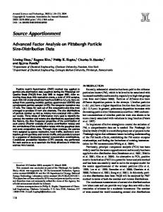
Figure S1. Wind-roses showing the frequency (%) of prevailing wind directions during the sampling periods.
S5
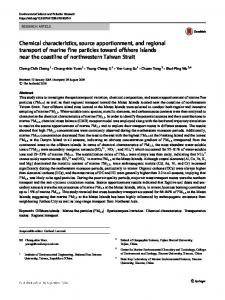
90
Concentration (ng m-3)
80 70 60 50 40 30 20 10 0
ACL
ACT
FLN
PHE
ANT
CRB
FL
PY
BaA
CHR
BaP
IcdP
DahA BghiP
Figure S2. Overall average concentrations (ng m-3) of individual PAHs (for all sites and seasons). Error bars indicate 1 SD. Acenaphthylene (ACL), acenaphthene (ACT), fluorene (FLN), phenanthrene (PHE), anthracene (ANT), carbazole (CRB), fluoranthene (FL), pyrene (PY), benz[a]anthracene (BaA), chrysene (CHR), benz[a]pyrene (BaP), indeno[1,2,3-c,d]pyrene (IcdP), dibenzo[a,h]anthracene (DahA). 4500 4000 3500
Concentration (pg m-3)
3000 2500 2000 1500 1000
0
PCB-18 PCB-17 PCB-31 PCB-28 PCB-33 PCB-52 PCB-49 PCB-44 PCB-74 PCB-70 PCB-95 PCB-101 PCB-99 PCB-87 PCB-110 PCB-82 PCB-151 PCB-149 PCB-118 PCB-153 PCB-132 PCB-105 PCB-138 PCB-158 PCB-187 PCB-183 PCB-128 PCB-177 PCB-171 PCB-156 PCB-180 PCB-170 PCB-199 PCB-194 PCB-206
500
Figure S3.Overall average concentrations (pg m-3) of individual PCBs (for all sites and seasons). Error bars indicate 1 SD.
S6
Contributions (ng m-3)
(a) Summer
700
Unburned crude oil and petroleum products
Diesel exhaust emissions
Gasoline exhaust emissions
Iron-steel production
Biomass/Coal combustion
600 500 400 300 200 100 0
(b) Fall
Contributions (ng
m-3)
700
Unburned crude oil and petroleum products
Diesel exhaust emissions
Gasoline exhaust emissions
Iron-steel production
600 500 400 300 200 100 0
Figure S4. Seasonal variation of source contributions to the Σ14PAH concentrations (ng/m3) in the study area.
S7
Biomass/Coal combustion
(c) Winter
Contributions (ng m-3 )
700
Unburned crude oil and petroleum products Gasoline exhaust emissions
Diesel exhaust emissions Iron-steel production
Biomass/Coal combustion
600 500 400 300 200 100 0
(d) Spring
Contributions (ng m-3)
700
Unburned crude oil and petroleum products Gasoline exhaust emissions
Diesel exhaust emissions Iron-steel production
600 500 400 300 200 100 0
Figure S4. Continued.
S8
Biomass/Coal combustion
(a) Summer
Coal and wood combustion
Technical PCB mixtures
Iron-steel production
Contributions (pg m-3)
35000 30000 25000 20000 15000 10000 5000 0
(b) Fall
Coal and wood combustion
Technical PCB mixtures
Contributions (pg m-3)
35000 30000 25000 20000 15000 10000 5000 0
Figure S5. Seasonal variation of source contributions to the Σ35PCB concentrations (pg/m3) in the study area. S9
Iron-steel production
(c) Winter
Contributions (pg m-3)
35000
Coal and wood combustion
Technical PCB mixtures
Iron-steel production
Coal and wood combustion
Technical PCB mixtures
Iron-steel production
30000 25000 20000 15000 10000 5000 0
(d) Spring
Contributions (pg m-3)
35000 30000 25000 20000 15000 10000 5000 0
Figure S5. Continued.
S10