Support Vector Machine Classification for Large Datasets Using ...

Support Vector Machine Classification for Large Datasets Using Decision Tree and Fisher Linear Discriminant Asdr´ ubal L´opez Chaua,b , Xiaoou Lib , Wen Yuc a

Universidad Aut´ onoma del Estado de M´exico, CU UAEM Zumpango, Zumpango Edo Mex, 55600, M´exico b Departamento de Computaci´ on, CINVESTAV-IPN, Mexico City, 07360, M´exico c Departamento de Control Autom´ atico, CINVESTAV-IPN, Mexico City, 07360, M´exico

Abstract The training of a support vector machine (SVM) has a time complexity between O(n2 ) and O(n3 ). Most training algorithms for SVM are not suitable for large data sets. Decision trees can simplify SVM training, however the classification accuracy becomes lower when there are inseparable points. This paper introduces a novel method for SVM classification. A decision tree is used to detect low entropy regions in input space. We use Fisher’s linear discriminant to detect the data near to support vectors. Experimental results demonstrate that our approach has good classification accuracy and low standard deviation, the training is significantly faster than other training methods. Keywords: Support vector machine, decision tree, Fisher linear discriminant 1. Introduction Support vector machine (SVM) is a well known classifier due to its excellent classification accuracy, generalization and compact model. It offers a hyperplane that represents the largest separation (or margin) between two classes [4]. In the linearly separable case the hyperplane is easy to compute, however in the general case it is necessary to use a soft margin SVM by introducing slack variables. In this way it is possible to find a hyperplane that splits the examples as cleanly as possible. In order to find a separation hyperplane, Preprint submitted to Elsevier

it is necessary to solve a Quadratic Programming Problem (QPP). This task is computational expensive, it has O(n3 ) time and O(n2 ) space complexities with n data [3]. The standard SVM is unfeasible for large data sets [20]. Many researchers have tried to find possible methods to apply SVM classification for large data sets. These methods can be divided into three types: a) reducing training data sets (data selection or data reduction) [14], b) using geometric properties of SVM [1], c) modifying SVM classifiers [24], April 22, 2013

d) decomposition [20]. Clustering is an effective tool to reduce data set size, for example, hierarchical clustering [15] and parallel clustering [19]. The sequential minimal optimization (SMO) [20] breaks the large QP problem into a series of smallest possible QP problems. The projected conjugate gradient (PCG) chunking scales somewhere between linear and cubic in the training set [8]. The random sampling method [14] is simple and commonly used for large data sets. However it needs to be applied several times, and the obtained results are not repeatable. Data selection methods choose objects which are support vectors (SV). These data are used for training the SVM classifier. Generally, the number of the support vectors is a small subset of the whole data [25]. The goals of this type of method are: (a) fast detection of support vectors (SV) which define the optimal separating hyperplane, (b) remove the data which are impossible to be SVs, (c) obtain similar accuracy using the reduced data set. In this paper, we use the data selection technique to train SVM with large data sets. Decision tree (DT) is classification method commonly used in many applications. A tree can be “learned” or induced by splitting the input space into subsets, based on an attribute value test. This process is repeated on each derived subset in a recursive manner [2]. Generally, the classification accuracy of SVM is better than DT. The training time of SVM is longer than DT for large data sets. The combination of SVM and DT can overcome two shortcomings of SVM: Computational burden and multiclass classification. In [7] each partition separated by a decision tree

is used to train SVM. It is similar with SMO, the large QP problem is transformed into several small SVMs by DT. In [13], the decision boundary of SVM is approximated by the boundaries of the decision tree. The multiclass SVM classification can be realized by the standard two-class classification by a binary tree [10]. There are two main problems: SVM has to be use to compute the margins at each leaf of DT [16]; the classification accuracy is poor when DT is not big enough [21], or the data are imbalance [27]. To improve the classification accuracy, the separability (margin measures) information are inserted in [5]. Fisher linear discriminant (FLD) is used to find a linear combination of features which separates two or more classes of objects. It is different from principal component analysis (PCA), in the last it is not an interdependence technique: a distinction between independent variables and dependent variables (also called criterion variables) must be made. In fact, SVM can be seen as a way to “sparsity” FLD [23]. FLD has been successfully applied in feature selection [26] and face recognition. The geometric properties of SVM can also be used to reduce the training data. In the linearly separable case, the maximum-margin hyperplane is equivalent to finding the closest pair of points in the convex hulls[1]. Neighborhood properties of the objects can be applied to detect SV and to improve classification accuracy of SVM. SVM with FLD uses the geometric properties of SVM. It is difficult to apply geometric properties in high-dimension and multiclass classification. While DT can overcome this disad2

where ξi > 0, i = 1 · · · n, are the slack variables, to tolerate mis-classifications. c > 0 is a regularization parameter. (3) is equivalent to the following dual problem with the Lagrange multipliers αi > 0 P P maxαi J(w) = − 21 ni=1,j=1 αi yi αj yj K hxi · xj i + ni=1 αi P such that : ni=1 αi yi = 0, C ≥ αi ≥ 0, i = 1, 2, . . . , n (4) with C > 0, αi ≥ 0, i = 1, 2, . . . , n, the coefficients corresponding to xi . All xi with nonzero αi are called support vectors. The function K is the kernel which must satisfy the Mercer condition [4]. The resulting optimal decision function is ! n X yi = sign αi yi K hxi · xj i + b (5)

vantage of SVM+FLD. In this paper, we use FLD to select part of data in each partition generated by DT. In this paper, we propose a novel data reduction method for SVM, it uses DT and FLD. The combination of decision tree and Fisher linear discriminant enable SVM for large data sets. With our method, low entropy regions in input space are detected. Only the data near to the support vectors are used to train SVM. We use 17 benchmark data sets to test our methods. The results show that our new classification method is very competitive compared with the other popular methods, such as LibSVM and SMO, especially for large data sets.

i=1

2. Three Classification SVM, DT, and FLD

Methods:

where x = [x1 , x2 , . . . , xn ] is the input data, αi and yi are Lagrange multipliers. A previously unseen sample x can be classified by (5). There is a Lagrangian multiplier α for each training point. When the maximum margin of the hyperplane is found, only the closed points to the hyperplane satisfy α > 0. These points are called support vectors (SV), the other points satisfy α = 0. So the solution is sparse. Here b is determined by Kuhn-Tucker conditions:

2.1. Support Vector Machine The training set X is given as X = {xi , yi }ni=1

(1)

where xi ∈ Rd , yi ∈ (1, .., CL ). The CL is the number of classes. Only continuous type attributes are used in this paper. SVM classifies data sets with an optimal separating hyperplane, which is given by T

w ϕ(xi ) + b

∂L ∂w

(2)

This hyperplane is obtained by solving the following quadratic programming problem P minw,b J(w) = 12 wwT + c ni=1 ξi (3) such that : yi wT ϕ(xi ) + b ≥ 1 − ξi

∂L ∂b

= 0, = 0,

∂L = ∂ξi 

αi 3

w= n X

n X

αi yi ϕ(xi )

i=1

αi yi = 0

i=1

0, αi − c ≥ 0   yi wT ϕ(xi ) + b ≥ 1 − ξi = 0

(6)

2.2. Decision Trees

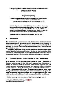
where atti is an attribute of training set X, the “split point00i is a value of the same type with the attribute i. The decision boundaries that are discovered by a decision tree are perpendicular to the axes of features. These boundaries can be seen as hyper rectangles. They are represented by the leaves L of T . A decision tree is shown in Figure 1.

When a data set X is large, the computational burden of (4) is heavy. We first use decision tree to separate X into several subsets. A decision tree is classifier whose model resembles a tree structure T , this structure is built from a labeled data set X. A decision tree is composed of nodes, and edges that connect the nodes. There are two type nodes: internal and terminal. The internal nodes have branches to connect to other ones, called its sons. The terminal nodes do not have any sons. A terminal node is called a leaf L of T . In general, a decision tree is generated by partitioning input data recursively into ”pure” regions with respect to certain measurement of the impurity. The measurements are defined in terms of instance distribution of the input splitting region. We use the following three impurity measurements: entropy, misclassification and the Gini impurities PCL −1 p(i|t)log2 p(i|t) Entropy(t) = − i=0 Classification error(t) = 1 − max[p(i|t)] P L −1 2 Gini = 1 − C i=0 [p(i|t)] (7) where CL is the number of classes, p(i|t) is the probability of of example i to be of the class t, which is the number of examples in the class t divided by the size of the set X, i =t| i.e., p(i|t) = |y|X| In order to create partitions in the input space, we use the following induction method atti < split pointi

Figure 1: Example of a decision tree

Any complex decision boundary can be approximated by using a large enough decision tree [9]. However, large decision trees can yield an over-fitting problem. The pruning method can be used to solve over-fitting in decision trees. There are two basic strategies to prune a decision tree: pre-pruning and post-prunning. The former strategy uses a criterion to stop the branch growing. The second strategy allows the tree to grow completely and then adjust it. In this paper, we use the post-pruning strategy, like C4.5 [21] and CART [2], because it is easy to obtain a (8) desired accuracy. 4

2.3. Fisher Linear Discriminant

lowing optimization problem

Although the decision tree method can |m+ − m− |2 (10) max J(ω) = help SVM to solve the computation problem s˜2+ + s˜2− ω for large data sets, the quadratic programming (4) is still slow, because SVM has to be Or equivalently solving applied to all data of each node of the deciω T SB ω sion tree [16]. Base on the geometric propermax J(ω) = T (11) ω S ω W ω ties of SVM, we use Fisher linear discriminant method to find the most possible data. We where only use these data for SVM training. + + |X |X P| T P| Considering a binary classification prob1 + T 1 m = |X + | ω x = ω |X + | x = ω T µ+ lem, i.e., the training data set X in (1) has i=1 i=1 − − |X |X CL = 2 (two classes). Let’s separate X into P| T P| 1 − T 1 + − m = |X − | ω x = ω |X − | x = ω T µ− two subsets X and X . i=1

X + = {xi ∈ X s.t. yi = c1 } X − = {xi ∈ X s.t. yi = c2 }

i=1

SB = (µ− − µ+ )(µ− − µ+ )T is called the between-class covariance matrix, P SW = P (xi − µ+ )(xi − µ+ )T + (xj −

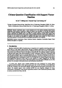
The Fisher’s linear discriminant method xi ∈X + xj ∈X − T searches for a vector ω that maximizes the µ− )(xj − µ− ) is called the total within-class separation between the means of X + and X − , covariance matrix. and at the same time that minimizes their The solution of (11) is given by scattering. In order to measure the scattering −1 ω = SW (µ+ − µ− ) (12) of X + and X − , the scatter s˜2 for projected objects on ω is defined as This solution can be obtained in O(d2 |X|). + An example of FLD is shown in Figure 2. |X P| 1 2 (yi − µ+ ) s˜+ = |X + | i=1 − |X P|

3. Support Vector Machine with Decision Tree and Fisher Linear Discrimi=1 − + inant |X |X P| P| µ− = |X1− | x, x ∈ X − , µ+ = |X1+ | x, x ∈ X + According to the geometric properties of i=1 i=1 (9) SVM, the separating hyperplane of SVM is where |X| is the cardinality or number of based on the support vectors which is a small elements in set X. s˜2 is also called within- subset of whole data. The support vector are class variance [3]. close to their opposite class, i.e., the support The vector ω is obtained by solving the fol- vectors are near to the boundaries [25] [12] s˜2− =

1 |X − |

(yi − µ− )

5

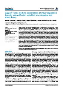
n the size of training set and d the number of features. 3) Search the data with shorter distances. We apply the Fisher’s linear discriminant to each pair of adjacent low entropy regions. The use of this linear discriminant is based on the fact that for linearly separable cases, the discriminant produces similar results of SVM [23]. Now we select the closest data between these regions. The selected data are called reduced data set XR . Once two adjacent regions have been detected, all the points in Lj are projected on vector ω,see (12). The data with the shortest projections are added to the reduced set XR . The total number of datum is d × |Lj |, where |Lj | is the data number in the leaf Lj , d is the dimension of the data of the induced tree T . It is important to notice that high entropy regions will contain support vectors, they do not need to be analyzed with Fisher linear discriminant in Step 3, but they are included directly in XR . Algorithm 1 shows the pseudo code of the proposed method. We use a simple example to show how our algorithm works. The data set used in the explanation is shown in Figure 3.

Figure 2: Example of Fisher’s linear discriminant in two dimensions, the black line is vector ω. Examples are projected on it.

[22]. The aim of using the decision tree and the Fisher linear discriminant is to find the data which are near to the support vectors. Our classification strategy can be divided in the following steps: 1) Discover regions that contain all or most of their examples with the same label. This label is the majority class for that region. 2) For each region, we determine all its adjacent or neighbor regions whose majority class is opposite. This is because we are interested in detecting data that are located to others with opposite label. Let’s T represent an induced decision tree, and Li a leaf of T . The leaves of T can be considered the low entropy regions that we need for implementing our strategy. After training a decision tree T , we detect the adjacent regions which contain opposite majority class in each region (leaf) Li . The decision tree partitions the input space such that it has lower entropy value. This partition needs O(n·d) time with

After the decision tree is trained, the input space is partitioned into six regions L1 to L6 . Each region is associated to a majority class y = {C1 , C2 }, with C1 = +1 or C2 = −1. Table 1 shows the discovered partitions, the majority class, and the adjacent regions. For a region Li , we use FLD to select the data which are close to adjacent regions Lj , that contain different class examples. For example, for region L4 (y = −1) the adjacent 6

Algorithm 1: General Algorithm 1 Input: X: Training set. δ: Threshold. Output: XR : XR ⊂ X s.t. |XR |  |X|. Begin Train a decision tree T ; // XR Begins empty XR ← N U LL For each leaf Li of T do 2 for each opposite class neighbor Lj do 3 if entropy of Lj is low then 4 //Select closest examples 5 Use Li and Lj to build X + ; 6 Compute ω (eq. (12)); 7 Add xi ∈ Lj to XR according to (12); 8 end for 9 else 10 //Add all the elements in Lj to XR . 11 XR ← XR ∪ L j ; 12 end if end for return XR End

Figure 3: Decision boundaries for SVM and Decision Tree classifiers

regions are L1 , L3 and L6 (y = +1). The region with high entropy value such as the L2 in Figure 3 is added directly to XR . 3.1. Adjacent regions

Detecting the adjacent regions is the key step in Algorithm 1. The leaves of an induced decision tree represent partitions or regions of input space. A decision tree splits the input space into low entropy regions, which are repTable 1: Partition of input space and adjacent regions resented as a leaf (terminal node) in the tree’s Region Majority class Adjacent regions structure. The leaves can be represented by L1 +1 L2 , L3 , L4 ( d ) L2 mixed L1 , L4 ,L5 \ L3 +1 L1 , L4 Li = rij , lij ≤ rij < hij (13) L4 -1 L1 , L2 , L3 ,L5 , L6 j=1 L5 -1 L2 , L4 , L6 where Li is the i − th leaf in the decision tree, L6 +1 L4 , L5 d is the dimension number of the training set, rij is a region of input space determined by 7

boundaries [lij , hij ), lij , hij ∈ R are the cutDefinition 2 Two leaves Lo and Lp are ting points found by an induction tree algo- neighbors if Lo ∪ Lp is a connected space. rithm. Property. Leaves Figure 4 shows a two-dimensional example, Lo and Lp are neighbors if exists m with 1 ≤ m ≤ d, and the follow are satisfied hom = lpm or lom = hpm lpn ≤ lon ≤ hpn or lpn ≤ hon ≤ hpn

(15) (16)

where 1 ≤ n ≤ d, n 6= m If two leaves Lo and Lp are neighbors, then there exists at least one point xn that satisfies xn ∈ {rok ∩ rpk }, f or k = 1, ..., d

(17)

This means that Lo and Lp must necessarily share a boundary or separating hyperplane which is orthogonal to an axis of features, for example m. The possible options are that the lower(upper) bound of Lp coincide with the upper(lower) bound of Lo , as in (15). Remark 2. The condition (15) is necessary, but not sufficient for two leaves to be neighbors. They need to share boundaries at the other dimensions. In order to fulfill (17), (16) must also be satisfied. We give an example to explain how to find the neighbors, see Figure 5. Here h1,1 = l5,1 (the separating hyperplane orthogonal to dimension one is shared by leaves L1 and L5 ), but L1 and L5 are not neighbors. Similarly, this occurs with the pairs (L1 ,L6 ), (L1 ,L7 ), (L2 ,L7 ), (L3 ,L5 ), (L3 ,L6 ), (L4 ,L6 ), (L4 ,L8 ) and (L5 ,L3 ). In Figure 6, the neighbors of L1 are L2 , L3 and L4 ; the neighbors of L2 are L1 , L3 , L4 , L5 and L6 .

Figure 4: Leaf Li with d = 2.

The regions detected by a decision tree have their boundaries defined by separating hyperplanes which are orthogonal to axes [9]. These regions are the leaves of decision tree and they can be interpreted as orthogonal disjoints or hyper boxes. Definition 1 Two leaves Lo and Lp , are candidate to be neighbors if their boundaries are changed by nT o d Lo = r , l ≤ r ≤ h oj oj oj oj nTj=1 o (14) d Lp = r , l ≤ r ≤ h pj pj pj pj j=1 Remark 1. Most induction tree algorithms split input space using a rule of the form xi < C. In the Definition 1, the boundaries of leaves Lo and Lp are changed to give them a connection chance. 8

Figure 6: The structure of decision tree that produces partitions shown in Fig. 5 Figure 5: Example of the boundaries produced by an induction tree algorithm

The second step is to compute the neighbors of any leaf Lp , see Algorithm 3. The The algorithm proposed in this paper to leave set SL satisfies (15) for an attribute m compute all the neighbors of a leaf includes in the matrix M . SL is explored again to find those leaves that are neighbors, namely, those two steps. The first step is to determine the bound- that satisfy (16). aries of each leaf, see Algorithm 2. All these boundaries are stored in a matrix M ∈ 4. Experiment results RNL ×2d , NL is the number of leaves in the In this paper our algorithm is compared induced decision tree. The i − th row in M contains the boundaries of leaf i. The first d with SMO [20], LibSVM [6] and Pegasos [29]. SMO was developed in 1998, it is the most columns of T contain the values lij , whereas the columns d + 1 upto 2d contain the val- representative method for training SVM. ues hij . The values lij and hij of a leaf are SMO is currently used to compare novel alimplemented as a vector, called B which is gorithms to train SVM. It uses the extreme initialized with the minimum and maximum case of decomposition approach , it modifies value representation of float point variables only a subset (known as the working set) of Lagrange multipliers per iteration, the size at root node. 9

Algorithm 2: Computation of leaves’ boundaries 1 Input: 2 T An induced decision tree. 3 Output: 4 M A matrix with the boundaries of all the leaves of T. 5 Begin 6 Initialize B as explained in the paper; 7 call BuildBoundaries(B,M) on root node; 8 return M; 9 End 10 11 12

13 14

15

16

17

18

19

20 21

Procedure BuildBoundaries(B, M) if current node is a leaf then Insert vector B as last row into matrix M ; else Create BL copying boundaries from B; BL : Change hij using attribute index and and split point value of current node; call BuildBoundaries(BL , M) on the left son of current node; Create BR copying boundaries from B; BR : Change lij using attribute index and and split point value of current node; call BuildBoundaries(BR , M) on the right son of current node; end if return

Figure 7: Checkerboard data set

Algorithm 3: Neighbors of a leaf 1 Input: 2 M matrix of leave’s boundaries. 3 Lp A leaf 4 Output: 5 N The neighbors of leaf Lp 6 Begin 7 for each attribute m 8 Get all leaves that satisfy (15); 9 for each leaf Lo gotten in the previous step 10 if Lo satisfies (16) then 11 Add to list N ; 12 end if 13 end for 14 end for 15 Remove repeated elements in N ; 16 return N ; 17 End

10

of working set is two. This leads to a small sub-problem to be minimized in each iteration. Because only two variables are involved in the optimization problem, it is not necessary to use any optimization software. In general, an advantage of decomposition methods is that they can deal with large data sets, because only a portion of training set is loaded in memory. A disadvantage of decomposition is that the convergence can be slow because selecting elements that form the working set is costly. LibSVM is a library updated in 2011 and used to train SVM with large data sets, it uses an method that implements an SMOtype algorithm. The main improvement of LibSVM over SMO is that the former uses a Hessian matrix (second order information) to select the elements of working set by detecting the points that most violate the KarushKuhn-Tucker conditions. Currently LibSVM one of the fastest methods for training SVM, it outperforms PSVM [17] and LS SVM [24]. Pegasos [29] is an algorithm developed in 2007 which alternates between stochastic gradient descent steps and projection steps. The algorithm has a small training times for large data sets. Pegasos achieves state-of-the-art results if Linear kernel is used, in the case of non linear kernel, Pegasis finds an approximated solution of the QP problem. All original data are applied to SMO and LibSVM training. The experiments are run on a computer with the following features: Core i7 2.2 GHz processor, 8.0 GB RAM, Windows 7 ultimate operating system. The algorithms are implemented in the Java language. The maximum amount of random ac-

cess memory given to the Java virtual machine is set to 2.0 GB. The results obtained in this paper correspond to 100 runs of each experiment. For each experiment, the training data are chosen randomly from 70% of the data set, the rest data are used for testing. The kernel used in all experiments is a radial basis function ! (x − z)T (x − z) (18) f (x, z) = exp − 2γ 2 where γ was selected using the grid search method. 4.1. Datasets In this paper we use 18 data sets to compare our method with the other ones. Nine data sets are public available, they are Haberman’s survival, Ionosphere, Breast cancer, Diabetes, Four-class, IJCNN-1, Bank marketing, Cod-RNA, and Skin Segmentation. Three data sets are modified for binary classification problems, they are Checkerboard [11] (see Figure 7), Iris, and Waveform. One data set is created artificially, it is Rotated cross (see Figure 8). The Table 2 shows a summary of the data sets used in the experiments. The Size is the number of examples in data set; Dim is the number of features; |yi = +1| and |yi = −1| is the number of data with label +1 and −1 respectively. 4.2. Parameters The parameters of our algorithms are the minimum number of objects in each leaf of

11

Table 2: Datasets for experiments Dataset Iris-setosa Iris-versicolor Iris-virginica Haberman’s Survival Ionosphere Breast-Cancer Diabetes Four-class Waveform-0 Waveform-1 Waveform-2 ijcnn1 Bank marketing Cod-rna Cross rotated Checkerboard100K Skin Segmentation

Figure 8: Rotated-cross data set

a decision tree (Min obj) and the fraction of examples that are taken from each region (δ). In order to achieve the best classification accuracy, the parameters of our algorithm need to be tuned. Table 3 shows the values used for each data set in the experiments. These values are selected by a grid searching method, which is widely used in the literature [3][23][24]. In Table 3, the regularization parameter for the QPP and the gamma for the kernel are represented by C and γ respectively. 4.3. Results The performances of SMO, LibSVM and our algorithm DTSVM are shown in the Table 4. It can be seen that the training time is improved in practically all cases with our method DTSVM. For small data sets, the time saving is not considerable. However, when the training sets are large, the computation burden is very low. The accuracies achieved by our algorithm are slightly de-

Size 100 100 100 306 351 683 768 862 3, 308 3, 347 3, 347 35, 000 45, 211 59, 535 90, 000 100, 000 245, 057

Dim |yi = +1| |yi = −1| 4 4 4 3 34 10 8 2 40 40 40 22 16 8 2 2 3

50 50 50 225 126 444 500 307 1, 653 1, 692 1, 692 3, 415 39, 922 19, 845 50, 000 50, 000 50, 859

50 50 50 81 225 239 268 555 1, 655 1, 655 1, 653 31, 585 5, 289 36, 690 40, 000 50, 000 194, 198

graded, but they are still acceptable. These are caused by the fact that some SV are not selected during the pre-processing step. The parameter C in our method is larger than LibSVM and SMO, because the training data of algorithm have more mixed samples. It is necessary to penalize the selected samples to obtain a good accuracy level. The size of training sets are reduced in about 80% to 90% for most cases. This reduction makes the training procedure faster for the large data set. The figure 9 shows the training times, these correspond to data sets larger than 1, 000. It can be seen that our DTSVM easily outperforms LibSVM and SMO. Pegasos has almost the same training time than our method. In some cases the training time using DTSVM is no better than Pegasos, however the accuracy obtained with our method is in general higher than the obtained with Pegasos, this can be seen in the figure 10.

12

Table 3: Value of parameters for the experiments Method LibSVM DTSVM LibSVM DTSVM LibSVM DTSVM LibSVM DTSVM LibSVM DTSVM LibSVM DTSVM LibSVM DTSVM LibSVM DTSVM LibSVM DTSVM LibSVM DTSVM LibSVM DTSVM LibSVM DTSVM LibSVM DTSVM LibSVM DTSVM LibSVM DTSVM LibSVM DTSVM LibSVM DTSVM

Dataset Iris-setosa

C

3.00 2.00 Iris-versicolor 1.00 3 Iris-virginica 1.00 3.00 Haberman’s survival 3.00 2.00 Ionosphere 2.50 3.00 Breast-cancer 1.00 1.50 Diabetes 1.00 2.5 Four-class 2.00 20.00 Waveform-0 1.00 2.50 Waveform-1 1.00 2.50 Waveform-2 1.00 2.50 ijcnn1 3.00 5.00 Bank marketing 3.50 4.30 cod-rna 4.50 10.50 Rotated Cross 2.00 3.00 Checkerboard100K 2.00 20.00 Skin Segmentation 1.00 2.00

γ

δ

Min obj

RBF Kernel

Algorithm 1

C4.5

3.00 1 3.00 1 3.00 1 2.00 2.00 1.55 2.00 1/n 1/n 1/n 2.00 3.00 3.50 1/n 1/n 1/n 1/n 1/n 1/n 1/n 1/n 2.3 1/n 3.5 3.5 1/n 1/n 3.00 3.50 1/n 1/n

0.10 0.10 0.15 0.30 0.50 0.50 0.15 0.15 0.35 0.35 0.35 0.10 0.05 0.35 0.15 0.35 0.15

2 2 2 15 2 10 5 2 35 35 35 30 40 100 20 2 25

Figure 9: Comparative of training times. The LibSVM and SMO run out of memory for the bank marketing data set.

5. Conclusions This paper proposes a novel method for SVM classification, DTSVM. By using decision trees (DT) and Fisher linear discriminant (FLD), DTSVM overcomes the problems of slow training of SVM and low accuracy of many DT and FLD based SVMs. The key point of our method is to find the low entropy regions and opposite class regions which are closed to decision boundaries. Experimental results demonstrate that our approach has good classification accuracy while

the training is significantly faster than other SVM classifiers. We compared DTSVM with other three methods of the state of the art, they are SMO, LibSVM library and Pegasos. Our method outperforms all these methods in training time and/or accuracy. For small data sets, the accuracy of DTSVM is maintained slightly lower than the classical SVM classifiers which use the whole data set. However, in the case of larger data sets, the classification accuracy are almost the same or even better than the other SVMs, because we do not use soft margin method to deal with the misleading points.

13

[1] M.Berg,

O.Cheong,

M.Kreveld,

[5] J. Chen, C. Wang, and R. Wang, Combining support vector machines with a pairwise decision tree, IEEE Geoscience and Remote Sensing Letters, vol. 5, no. 3, pp. 409 –413, july 2008. [6] C. Chih-Chung and L. Chih-Jen, Libsvm: A library for support vector machines, ACM Transactions on Intelligent Systems and Technology, vol. 2, no. 3, pp. 1–27, 2011. [7] F. Chang, C.-Y. Guo, X.-R. Lin, and C.J. Lu, Tree decomposition for large-scale svm problems,J. Mach. Learn. Res., vol. 9999, pp. 2935-2972, December 2010.

Figure 10: Comparative of accuracies. The LibSVM and SMO run out of memory for the bank marketing data set.

[8] R.Collobert, S.Bengio, SVMTorch: Support vector machines for large regression problems, Journal of Machine Learning Research, Vol.1, 143-160, 2001. [9] R. O. Duda, P. E. Hart, and D. G. Stork, Pattern Classification (2nd Edition). Wiley-Interscience, 2000.

M.Overmars, Computational Geometry: Algorithms and Applications, Springer-Verlag, 2008 [10] B. Fei and J. Liu, Binary tree of svm: A new fast multiclass training and classifi[2] L. Breiman, J. H. Friedman, R. A. Olcation algorithm, IEEE Transactions on shen, and C. J. Stone, Classification and Neural Networks, vol. 17, no. 3, pp. 696 Regression Trees. Wadsworth, 1984. -704, may 2006.

[3] C. M. Bishop, Pattern Recognition and [11] T.Ho and E. Kleinberg, Checkerboard Machine Learning, Secaucus, NJ, USA: data set, http://www.cs.wisc.edu/mathSpringer-Verlag New York, Inc., 2006. prog/mpml.html, 1996. [4] N. Cristianini and J. Shawe-Taylor, An [12] S. Katagiri and S. Abe, “Selecting supIntroduction to Support Vector Machines port vector candidates for incre-mental and Other Kernel-based Learning Methtraining,” in Systems, Man and Cyberods, Cambridge University Press, Mar. netics, 2005 IEEE Inter-national Con2000. ference, vol. 2, oct. 2005, pp. 1258–1263. 14

[13] M.A.Kumar and M. Gopal, “A hy- [19] C.Pizzuti, D.Talia, P-Auto Class: Scalbrid svm based decision tree,” Pattern able Parallel Clustering for Mining Large Recogn., vol. 43, no. 12, pp. 3977–3987, Data Sets, IEEE Trans. Knowledge and Dec. 2010 Data Eng., vol.15, no.3, pp.629-641, 2003. [14] Y. Lee and O. L. Mangasarian, Rsvm: Reduced support vector machines, Data [20] J. Platt, Fast training of support vector machines using sequential min-imal opMining Institute, Computer Sciences timization, Advances in Kernel Methods: Department, University of Wisconsin, Support Vector Ma-chines, pp. pp. 185– 2001, pp. 100–107. 208, 1998. [15] X.Li, J.Cervantes, W.Yu, Fast Classifi[21] J. R. Quinlan, C4.5: Programs for Macation for Large Data Sets via Random chine Learning. San Mateo, CA: Morgan Selection Clustering and Support VecKaufmann, 1993. tor Machines, Intelligent Data Analysis, Vol.16, No.6, 897-914, 2012 [22] H. Shin and S. Cho, Neighborhood property-based pattern selection for sup[16] M. Lu, C. L. P. Chen, J. Huo, and X. port vector machines, Neural Comput., Wang, Multi stage decision tree based vol. 19, no. 3, pp. 816–855, March 2007. on inter-class and inner-class margin of svm, Proceedings of the 2009 IEEE in- [23] A. Shashua, “On the relationship between the support vector machine for ternational conference on Systems, Man classification and sparsified fisher’s linand Cybernetics, Piscataway, NJ, USA: ear discriminant,” Neural Process. Lett., IEEE Press, 2009, pp. 1875–1880. vol. 9, no. 2, pp. 129–139, Apr. 1999. [17] G. Fung and O. L. Mangasarian, Proxi[24] J.A.K.Suykens , J.Vandewalle , Least mal Support Vector Machine Classifiers, squares support vector machine classiProceedings KDD-2001: Knowledge Disfiers, Neural Processing Letters, vol. 9, covery and Data Mining, August 26-29, no. 3, Jun. 1999, pp. 293–300. 2001, San Francisco, CA, 2001, pp. 77– 86 [25] D. M. J. Tax and R. P. W. Duin, “Support vector data description,” Mach. [18] Michael E. Mavroforakis and Margaritis Learn., vol. 54, no. 1, pp. 45–66, Jan. Sdralis and Sergios Theodoridis, A Geo2004. metric Nearest Point Algorithm for the Efficient Solution of the SVM Classifica- [26] E.Youn, .Koenig, M. K.Jeong, .H. Baek tion Task, IEEE Transactions on Neural , Support vector-based feature selection Networks, Vol. 18, 2007, pp. 1545–1549 using Fisher’s linear discriminant and 15

Support Vector Machine, Expert Systems with Applications, Volume 37 Issue 9, 6148-6156, 2010 [27] H. ZHAO, Y. YAO, AND Z. LIU, A classification method based on non-linear svm decision tree, in Proceedings of the Fourth International Conference on Fuzzy Systems and Knowledge Discovery , 2007, pp. 635–638. [28] C.ZHOU, X.WEI, Q.ZHANG, X.FANG, Fisher’s linear discriminant (FLD) and support vector machine (SVM) in nonnegative matrix factorization (NMF) residual space for face recognition, Optica Applicata, Vol. XL, No. 3, 2010 [29] SHALEV-SHWARTZ, SHAI AND SINGER, YORAM AND SREBRO, NATHAN, Pegasos: Primal Estimated sub-GrAdient SOlver for SVM, Proceedings of the 24th international conference on Machine learning, 2007, isbn 978-159593-793-3,Corvalis, Oregon, USA. pp. 807–814

16

Table 4: Performance Method

Dataset

LibSVM SMO Pegasos DTSVM LibSVM SMO Pegasos DTSVM LibSVM SMO Pegasos DTSVM LibSVM SMO Pegasos DTSVM LibSVM SMO Pegasos DTSVM LibSVM SMO Pegasos DTSVM LibSVM SMO Pegasos DTSVM LibSVM SMO Pegasos DTSVM LibSVM SMO Pegasos DTSVM LibSVM SMO Pegasos DTSVM LibSVM SMO Pegasos DTSVM LibSVM SMO Pegasos DTSVM LibSVM SMO Pegasos DTSVM LibSVM SMO Pegasos DTSVM LibSVM SMO Pegasos DTSVM LibSVM SMO Pegasos DTSVM LibSVM SMO Pegasos DTSVM

Iris-setosa

Training avg (ms) 3.11 3.01 0.10 0.88 Iris-versicolor 1.51 1.65 0.11 1.35 Iris-virginica 1.76 1.68 0.07 1.43 Haberman’s survival 9.48 10.51 9.01 4.51 Ionosphere 9.48 8.59 50.00 4.51 Breast-cancer 29.36 0.35 80.00 15.78 Diabetes 81.13 35.00 90.00 15.00 Four-class 18.10 21.23 29.12 14.06 waveformBin-0 1, 210.40 1, 687.00 410.21 193.30 waveformBin-1 1, 659.50 1, 840.00 420.18 316.60 waveformBin-2 1, 667.00 1, 859.00 421.01 193.00 ijcnn1 25, 875.25 48, 923.31 3, 720.06 5, 444.25 Bank marketing mem error mem error 7, 440.00 5, 444.25 cod-rna 441, 568.70 989, 476.00 3, 420.12 23, 224.7 Rotated Cross 119, 123.14 309, 111.00 2, 450.00 6, 726.91 Checkerboard100K 131, 855.25 285, 621.12 2, 536.64 8, 740.25 Skin Segmentation 131, 855.25 302, 670.83 6, 240.25 8, 740.25

Training stdev 2.45 2.33 1.02 3.82 2.33 3.10 1.12 3.75 2.42 2.48 0.95 4.01 7.89 6.55 5.25 8.87 7.89 9.91 8.15 8.87 1.95 1.45 6.34 7.64 6.27 7.12 7.15 14.77 5.87 8.51 8.15 17.14 180.69 78.96 45.36 66.57 49.39 33.89 117.15 168.59 42.85 30.55 110.49 75.55 3, 650.04 4, 605.03 256.01 375.03

135.48 375.03 33, 942.69 89, 279.26 453.01 11, 866.53 22, 368.78 2, 078.03 1, 968.48 2, 400.82 3, 116.76 4, 036.99 891.02 412.39 3, 116.76 2, 889.00 489.93 412.39

Acc Acc avg (%) stdev 94.65 0.03 94.70 0.02 95.00 0.12 89.21 0.19 100.00 0.00 100.00 0.00 100.00 0.00 100.00 0.00 100.00 0.00 100.00 0.00 100.00 0.00 100.00 0.00 73.41 0.03 73.55 0.03 72.59 0.08 73.08 0.06 91.41 0.03 90.05 0.03 89.17 006 77.35 0.06 96.63 0.01 96.92 0.01 96.77 0.08 97.31 0.08 74.73 0.02 77.34 0.03 77.73 0.05 73.25 0.08 99.81 0.00 98.78 0.02 77.14 0.12 97.55 0.04 94.39 0.01 93.99 0.02 93.95 0.04 93.78 0.01 92.52 0.02 92.60 0.00 92.02 0.01 91.31 0.01 92.50 0.01 92.70 0.02 92.58 0.01 91.98 0.00 97.92 3.65 96.01 1.01 90.63 0.02 96.06 0.00

89.28 96.06 93.05 94.01 93.86 92.46 94.15 93.65 66.49 93.78 98.86 98.99 50.66 97.15 98.86 98.10 92.89 97.05

0.13 0.00 0.01 0.02 0.15 0.01 0.02 0.01 0.25 0.02 5.79 0.01 0.15 0.00 5.79 0.03 0.06 0.00

Size reduced (%) 79.46 68.19 68.04 80.52 82.73 84.51 84.46 70.49 88.22 64.01 89.98 89.96 89.96 87.67 92.53 89.99 89.99