Support Vector Reduction in SVM Algorithm for ... - Semantic Scholar

606

IEEE GEOSCIENCE AND REMOTE SENSING LETTERS, VOL. 6, NO. 3, JULY 2009

Support Vector Reduction in SVM Algorithm for Abrupt Change Detection in Remote Sensing Tarek Habib, Member, IEEE, Jordi Inglada, Associate Member, IEEE, Grégoire Mercier, Senior Member, IEEE, and Jocelyn Chanussot, Senior Member, IEEE

Abstract—Satellite imagery classification using the support vector machine (SVM) algorithm may be a time-consuming task. This may lead to unacceptable performances for risk management applications that are very time constrained. Hence, methods for accelerating the SVM classification are mandatory. From the SVM decision function, it can be noted that the classification time is proportional to the number of support vectors (SVs) in the nonlinear case. In this letter, four different algorithms for reducing the number of SVs are proposed. The algorithms have been tested in the frame of a change detection application, which corresponds to a change-versus-no-change classification problem, based on a set of generic change criteria extracted from different combinations of remote sensing imagery. Index Terms—Image classification, image matching, image processing, remote sensing.

I. I NTRODUCTION

I

N THE context of risk management and hazard assessment using satellite imagery, high-performing change detection algorithms are of great importance [1]. For this type of application, change detection problems can be viewed as a classification using two classes (change/no change). Due to its multiple advantages, the support vector machine (SVM) binary classification algorithm has been widely used for the classification of satellite imagery [2]. In this letter, the SVM algorithm is used in the context of building a generic change detection algorithm. In order to achieve the goal of genericity, a large amount of change indicators have been extracted from the images and used as input in the SVMs, yielding highdimensionality input vectors. Despite the fact that, theoretically, the SVM algorithm can handle such large data sets with high dimensionality, in practice, the following two main problems arise: 1) The computation time required for the convergence of the optimization problem during the “learning” step of the SVM algorithm is very high, and 2) the classification time Manuscript received September 5, 2008; revised January 19, 2009. Current version published July 4, 2009. T. Habib is with the Centre National d’Études Spatiales, Direction du Centre de Toulouse/Système et Images/Analyse et Produits Images (DCT/SI/AP), 31401 Toulouse, France, and also with the Images and Signal Department, GIPSA-lab, 38402 Grenoble Cedex, France. J. Inglada is with the Centre National d’Études Spatiales, Direction du Centre de Toulouse/Système et Images/Analyse et Produits Images (DCT/SI/AP), 31401 Toulouse, France. G. Mercier is with the Laboratoire des Sciences et Technologies de l’information, Communication and Knowledge, Centre National de la Recherche Scientifique Unité Mixte de Recherche, Telecom Bretagne, Institut Telecom, 29238 Brest Cedex 3, France. J. Chanussot is with the Images and Signal Department, GIPSA-lab, 38402 Grenoble Cedex, France. Color versions of one or more of the figures in this paper are available online at http://ieeexplore.ieee.org. Digital Object Identifier 10.1109/LGRS.2009.2020306

increases in a polynomial fashion with the increase in the data dimensionality [3]. This letter focuses on the decrease of the classification time. In the SVM algorithm, the classification time is directly proportional to the number of support vectors (SVs) in the nonlinear case. Several methods for the SV reduction are proposed in Section III. The reduction of the SVs may logically result in a decrease in the classification accuracy; however, in the context of risk management and hazard assessment, a slight decrease in the classification accuracy can be tolerated for a gain in classification time. This letter is divided into the following sections. In Section II, a brief introduction on the SVM binary classification algorithm is presented. In Section III, the proposed techniques for obtaining the reduced set of SVs are presented. The conducted experiments and the results obtained using the different methods are discussed in Section IV. Finally, the conclusions are drawn in Section V. II. SVM S The SVMs are state-of-the-art large margin classifiers that have gained much popularity within the image-processing community. The SVM is a learning-based binary classification algorithm that is based on the concept of structural risk minimization [4]. This construction has shown to generally outperform traditional learning machines like multilayer neural networks that are based on the concept of empirical risk minimization [5]. In this section, a brief review of the theory of this algorithm is presented; for further details, the reader is invited to review [6]. n Consider a set of learning data (xi , yi )m i=1 , where xi ∈  are the input feature vectors, and yi ∈ {−1, +1} are the set of corresponding labels (i.e., classes). The SVM solution finds ytest = f (xtest ) for a new test vector xtest so that the probability of the error is minimal. The SVM decision for any new vector xtest is obtained under the hypothesis that xtest is issued from the same unknown probability density function that produced the learning set xi . If it is assumed that the two classes (i.e., the SVM is a binary classifier) can be separated by a hyperplane and that no prior information concerning the data distribution is available, then the optimal hyperplane is the one which maximizes the margin of separation between the two classes [6]. The optimal values of w and b can be obtained by solving a constrained minimization problem through the use of the Lagrange multipliers αi . The decision function provided by the SVM can thus be put in the following form: m   αi yi K(xtest , xi ) + b . (1) f (xtest ) = sgn i=1

1545-598X/$25.00 © 2009 IEEE

Authorized licensed use limited to: Jocelyn Chanussot. Downloaded on August 20, 2009 at 07:21 from IEEE Xplore. Restrictions apply.

HABIB et al.: SUPPORT VECTOR REDUCTION IN SVM ALGORITHM

The input feature vectors xi having a Lagrange multiplier αi that is not equal to zero are considered as SVs, hence the name SVMs. The kernel function K(·, ·) substitutes the scalar product ·, · in order to allow the SVM to learn the nonlinear classifiers as, for example, polynomial classifiers or radial basis function (RBF) networks. III. R EDUCED S ET OF SV With the goal of providing a tradeoff between the classification accuracy and the computation time, four different approaches are proposed in this section. The objective of these approaches is the selection of a representative subset of the SVs. These approaches are intended to select the SVs according to their importance in order to obtain an acceptable approximation of the SVM decision boundary. A. Set Reduction by Lagrange Multipliers The value of the Lagrange multipliers is a valid indicator of the importance of a given vector. Using the information provided by the Lagrange multipliers, the first approach would be to keep the SVs based on the value of the Lagrange multipliers. Thus, the SVs with the highest unbounded Lagrange multipliers (i.e., 0 < αi < C) will be used as the reduced set, and the rest of the SVs will be eliminated. The size of the reduced set is either specified a priori by a percentage of the entire set of SVs or by specifying a threshold on the value of the αi to be retained. If the percentage is higher than the available number of unbounded SVs, the set is completed using the randomly selected bounded SVs. Since this SV reduction procedure may not mrespect the constraints of the SVM algorithm, namely, i=1 αi yi = 0, then a new learning step has to be applied. A modified classification algorithm that takes into consideration the SVM constraints is proposed as follows: 1) Perform a first learning step; 2) choose a subset of the SVs according to a maximum value of the αi with αi < C; 3) reperform the learning step; and 4) classify. The added relearning step launches the learning process only on the chosen reduced set of vectors using the same kernel as the one used in the first learning step. Intuitively, since these vectors were already considered as SVs in the first learning step, then the optimization procedure will separate them similarly to the previous learning step, and thus, the role of the second learning step will be simply  to reattribute the values of the αi in order to guarantee m i=1 αi yi = 0. In practice, however, and due to the implementation issues of the SVM optimization, it was noted that a very limited number of vectors (basically two or three for a set of 600 SVs) are not considered as SVs anymore. It is not likely to have an impact on the overall classification performance since this quantity is negligible with respect to the total number of SVs. B. Set Reduction by Distance to Separating Surface The decision function as presented in (1) can be used to build a distance measure. The distance-to-hyperplane measure may be defined by fd (x) =

m  i=1

αi yi K(x, xi ) + b.

607

The SV’s relative position, with respect to the separating boundary, could be evaluated and then used as a criterion in the SV reduction. The procedures are: 1) Perform a first learning step; 2) choose a subset of the SVs according to a maximum value of fd (xi ) as in the aforementioned equation; 3) reperform the learning step; and 4) classify. As mentioned earlier, the relearned step is used in order to recompute the αi . As implemented in this algorithm, the SVs situated far away from the separating hyperplane are considered as better suited for set reduction since they provide a better generalization of the separating hyperplane. The situation far from the hyperplane limits the eventual overlap between the two classes and hence is expected to provide a better separability between the two classes. C. Set Reduction by Mechanical Analogy In [7], Schlkopf and Smola present the SVM classification problem as a mechanical problem. The structure of the SVM optimization problem is closely similar to the ones that typically arise in Lagrange’s formulation of mechanics. From this point of view, it is possible to give a mechanical interpretation to the optimal margin hyperplanes. Assume that each SV xi exerts a perpendicular force of magnitude αi and direction yi (w/w) on a solid plane sheet lying along the hyperplane. The idea is to use this mechanical analogy to reduce the number of SVs by merging the vectors using geometrical and mechanical properties. According to this point of view, two SVs x1 and x2 may be replaced by a new vector xnew if its mean is set as the mean of the two vectors. The difficult point would be to set the value of αnew , which is associated to xnew . Considering the mechanical analogy, the problem would be to identify the direction of this force (i.e., the vector that is perpendicular to the separating boundary w cannot be computed directly in the nonlinear case). This problem could be avoided by merging the two vectors directly in the feature space (i.e., the space induced by the kernel function). Assuming that the system is stable around the origin of the feature space, the αnew could be obtained as follows: αnew ynew K(xnew , xnew ) = y1 α1 K(x1 , x1 ) + y2 α2 K(x2 , x2 ).  Once again, in order to respect m i=1 αi yi = 0, the difference (i.e., δ) between the computed αnew and the required one for stability is computed by αnew ynew + δ = α1 y1 + α2 y2 .

(2)

Once the value of δ is obtained, it is distributed uniformly on the SVs of the same class of xnew [according to the sign of f (xnew ) in (1)], which guarantees the SVM stability constraint. An algorithm based on this mechanical analogy was developed. In order to identify the SVs that should be merged together, a specific signature was computed for each vector, and then, the vectors with similar signatures are merged. The proposed algorithm is decomposed in the following steps, which will be detailed further on: 1) Compute the signatures of the different SVs (sn ); 2) compute the distances between the different vectors according to their respective signature [D(si , sj )] by evaluating the symmetrized

Authorized licensed use limited to: Jocelyn Chanussot. Downloaded on August 20, 2009 at 07:21 from IEEE Xplore. Restrictions apply.

608

IEEE GEOSCIENCE AND REMOTE SENSING LETTERS, VOL. 6, NO. 3, JULY 2009

Kullback–Leibler (KL) distance; and 3) define a threshold and then merge the SVs having an interdistance that is less than the defined threshold. The signature sn of an SV xn is a vector of the m components (m is the number of SVs) defined, component by component, by the value of K(xi , xn ), 1  i  m

as follows (note that this computation can be extended to merge any number of vectors):

sn = (K(x1 , xn ), K(x2 , xn ), . . . , K(xm , xn )) .

(3)

The computation of the signature by using this procedure has two reasons: 1) The interaction between the different vectors using the kernel function is indicative of the distribution in the feature space, and 2) the kernel values are already computed during the learning phase, and hence, with proper storage, no further computation will be required. Once the signature for all the m vectors is computed, the symmetrized KL distance is used to identify the vectors to be merged. The expression of this distance was developed in [8] and is defined as follows: 1 1 1 = + R(s1 , s2 ) D(s1 s2 ) D(s2 s1 )

(4)

 where D(s1 s2 ) = s1 (x) log(s1 (x)/s2 (x))dx. The reason for using this type of distance instead of, for example, a simple quadratic distance is its interesting properties. This type of distance measurement is based on the KL divergence [9] that contains the discrimination information of the first hypothesis (i.e., represented by s1 ) on the second hypothesis (i.e., represented by s2 ). The addition of such a rich measurement that already contains information concerning the discrimination between the two classes can enhance the classification performance in the sense that it allows a first stage of clustering of the vectors. The threshold definition procedure can be done manually or automatically according to the required number of SVs at the output of this reduction process. This procedure has the advantage of not requiring a new learning step like the other algorithms; however, the computation of the signatures and the distances is a time-consuming task. Knowing that all these kernel evaluations have been already computed during the initial learning phase, storing these values greatly increases the speed of this algorithm. The total number of operations required for this algorithm is then (4m + 1) for the KL distance computation in addition to the six operations required to evaluate the values of αnew and xnew . On the other hand, merging two vectors saves the m operations for the classification of a new test vector. Thus, if N > (4m + 7), this type of reduced set SVM can be interesting, where N is the total number of test data vectors to be classified. D. Set Reduction by Optimization Problem Following the same procedure as that proposed for the mechanical analogy approach, another strategy may be used to evaluate αnew . It takes its inspiration from the SVM optimization problem in the sense that the solution of the SVM optimization problem using the new vector is equal to the solution obtained using the original vectors x1 and x2 . Once the values of ynew and xnew are specified, the αnew of the new SV xnew can be computed in order to replace the two SVs αi1 and αi2 . αnew can be obtained

αnew =

αi1 + αi2 − 12 (Ti1 + Ti2 + Ti1 ;i2 ) m  1 − 12 αi yi ynew K(xi , xnew ) i=1 i=i1 ,i2

where Ti1 ;i2 = 2αi1 αi2 yi1 yi2 K(xi1 , xi2 ), Ti =

m 

for i = i1 or i2

αj αi yj yi K(xi , xj ).

j=1 j=i1 i2

The number of operations required to compute αnew from the merging of the two vectors is (7m − 6); this includes the computation of the KL distance to identify the vectors to be merged. Thus, this type of reduction is interesting when N > (7m − 6), where N is the number of data vectors to be classified. When three vectors are merged using this technique, the reduction is interesting when N > (6m − 2); thus, the procedure becomes more interesting when the number of vectors to be merged increases. IV. E XPERIMENTS The proposed SV reduction algorithms were tested on three data sets. The first is the Goma data set that is composed of a pair of synthetic aperture radar images that were obtained before/after the Nyiragongo volcanic eruption in eastern Congo in 2002. The second set is composed of a pair of optical Satellite Pour l’Observation de la Terre images that were obtained before/after the earthquake that hit the Algerian city of Boumerdes. Several features were computed, namely, difference, ratio, ratio of means, ratio of medians, correlation, mean squares, KL distance, mutual information, cardinality match, gradient difference, entropy, and energy. Along with the original images, these images were used to form the input vectors for the SVM algorithm, with each feature representing one component of the vector; this yields vectors of size 14. For testing purposes, a soft margin SVM was used, with C = 1. An RBF kernel was used, with γ = 0.5 (i.e., it should be noted that the exact values of the parameters are of no interest in our case since we are only interested in obtaining information concerning the overall behavior of algorithms that are independent of these parameters). Ten different full iterations were performed on the test data. A single iteration is composed of the following steps: 1) Choose a random set of learning vectors (consisting 1% of the total number of available testing vectors); 2) perform the learning phase of the SVM algorithm in order to obtain the original SV set; 3) reduce the number of SVs by following the different algorithms (for the algorithm in Section III-A, this means 10% reduction with respect to the original set’s size, whereas for the remaining three algorithms, this means increase of the threshold by 10% of the maximum distance according to the specified criteria); 4) perform the SVM classification using the new sets (four new sets following the four proposed algorithms) of SVs; and 5) restart from step 3 until the new SV set’s size is only 10% of the original SV set.

Authorized licensed use limited to: Jocelyn Chanussot. Downloaded on August 20, 2009 at 07:21 from IEEE Xplore. Restrictions apply.

HABIB et al.: SUPPORT VECTOR REDUCTION IN SVM ALGORITHM

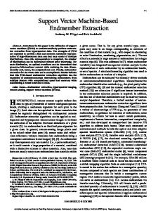
Fig. 1. Classification accuracy versus percentage (divided by ten) of the set’s size reduction with respect to the original set’s size using the reduced set algorithm of Section III-A applied on the different data sets. (a) Goma data set. (b) Boumerdes data set.

609

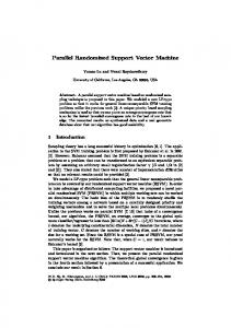
Fig. 2. Classification accuracy versus percentage (divided by ten) of the maximum distance using the reduced set algorithm defined in Section III-B. (a) Goma data set. (b) Boumerdes data set.

Note that, in the following figures, the green line is a simple connection between the mean values. This green line is intended to show the overall behavior of the different functions. A. Set Reduction by Lagrange Multipliers Fig. 1 shows the classification error using the reduced set as a function of the total number of SVs applied on the different testing data sets. Hence, the x-axis represents the percentage of SVs that was removed (×10). In the case shown in Fig. 1(a), the classification accuracy is almost constant with the removal of the SVs. However, due to the large variance of the classification error, following this method may not be robust to reduce the set from the Goma data. In the case shown in Fig. 1(b), the evolution is convenient in the sense that the classification accuracy decreases with the removal of the SVs. Thus, it offers a tradeoff between the classification accuracy and the classification time (through the reduction of the number of SVs). However, when removing a large number of SVs (i.e., higher than 70%), the variance of the classification accuracy is very high, showing that the results are more and more noisy. B. Set Reduction by Distance to Separating Surface Fig. 2 shows the results obtained for the algorithm using the distance-to-hyperplane criteria. From Fig. 2(a), the results show that the classification accuracy has a large variance with respect to the removal of the SVs. On the other hand, the mean values show that this technique can be used to provide a tradeoff between the classification accuracy and the classification time since the overall accuracy decreases with the decrease of the number of SVs. When tested on the Boumerdes data set as shown in Fig. 2(b), this approach provides irregular results, where the classification accuracy seems to be independent of the number of SVs.

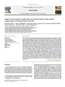
Fig. 3. Classification accuracy versus merging step using the algorithm of Section III-C. (a) Goma data set. (b) Boumerdes data set.

C. Set Reduction by Mechanical Analogy Fig. 3 shows the results obtained using the algorithm defined in Section III-C. It can be noticed that the error’s mean and variance increase with the number of merged vectors. As the number of SVs decreases, the separating surface becomes an approximation of the original surface and thus provides a lower classification accuracy. This shows that the reduced set using this technique can provide a tradeoff between the classification accuracy and the classification time through the reduction of the SVs. Despite a large variance of the classification accuracy, the reduced set using the mechanical analogy provides adequate results when applied to the Goma data set. As can be seen in Fig. 3(a), the classification accuracy slightly decreases with the decrease of the number of SVs. This is maintained until

Authorized licensed use limited to: Jocelyn Chanussot. Downloaded on August 20, 2009 at 07:21 from IEEE Xplore. Restrictions apply.

610

IEEE GEOSCIENCE AND REMOTE SENSING LETTERS, VOL. 6, NO. 3, JULY 2009

TABLE I AMOUNT OF REDUCTION OPPOSED TO THE AVERAGE CLASSIFICATION TIME (IN CPU TIME) FOR THE DIFFERENT SET REDUCTION TECHNIQUES

E. Classification Time

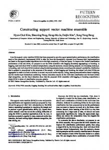
Fig. 4. Classification accuracy versus the merging step using the optimization problem algorithm. (a) Goma data set. (b) Boumerdes data set.

a very large number of SVs are removed (80%), where the classification result becomes unreliable due to the lack of representativeness of the remaining SVs. Fig. 3(b) shows the result obtained when the algorithm is applied on the Boumerdes data set. It can be noted that the algorithm provides reasonable results in terms of the variance of the classification accuracy as well as the accuracy with respect to the number of SVs that remains constant until 70% of the SVs are removed. D. Set Reduction by Optimization Problem Fig. 4 shows the results obtained using the algorithm defined in Section III-D. From these results, it can be shown that the mean error increases with the decrease of the number of SVs. However, the variance value remains high independently from the number of SVs. Fig. 4(a) shows the results of the application of the algorithm on the Goma data set. Despite a large variance of the classification accuracy, the algorithm provides good results, where the mean classification accuracy is being maintained at a relatively constant level with the removal of the SVs. Similar to the tests on the Goma data set are the tests on the Boumerdes data set. Fig. 4(b) shows that the algorithm is capable of preserving the classification accuracy despite the removal of the SVs. Hence, the obtained approximation of the separating hyperplane is satisfactory. After the inspection of the different obtained results, it can be observed that, in terms of classification accuracy, the mechanical-analogy-based algorithm provides the best results. The algorithm using the optimization problem is also efficient but suffers from the following two drawbacks: 1) high computational cost during the merging phase and 2) high error variance independently from the number of available SVs. The algorithms using the distance to the hyperplane and the direct filtering of the Lagrange multipliers provide irregular results, probably due to the relearn step that could change the shape of the separating hyperplane.

In this section, a comparison between the different methods is provided in terms of computational time. Table I shows the amount of reduction opposed to the average classification time As can be seen from these results, despite the computational cost added for the merging schemes represented by the optimization problem or the mechanical analogy set reduction techniques, the computation time reduction as proposed in these methods remains interesting. Note, however, that the computation time required for the filtering techniques (i.e., represented by the Lagrange multiplier set reduction and the distance-tohyperplane set reduction techniques) has a significantly less computation time, but, as shown earlier, this large decrease of the computation time comes at the expense of the classification accuracy. V. C ONCLUSION In this letter, four different SV set reduction algorithms have been proposed. The objective of these different algorithms is to accelerate the classification process for a generic SVM-based change detection algorithm in the context of risk management in order to respect crucial operational time constraints. Since the classification time is directly proportional to the number of SVs in the nonlinear case, the adopted strategy was to obtain a reduced set of the initial SVs. It was noted that the algorithms using the mechanical analogy (Section III-C) and the optimization problem (Section III-D) show good performances. The algorithm using the mechanical analogy provides the best results since it overperforms the algorithm using the optimization problem both in required computation and in the classification accuracy. R EFERENCES [1] T. Habib, J. Chanussot, J. Inglada, and G. Mercier, “Abrupt change detection on multitemporal remote sensing images: A statistical overview of methodologies applied on real cases,” in Proc. IEEE IGARSS, Barcelona, Spain, Jul. 2007, pp. 2593–2596. [2] N. Ghoggali and F. Melgani, “Genetic SVM approach to semisupervised multitemporal classification,” IEEE Geosci. Remote Sens. Lett., vol. 5, no. 2, pp. 212–216, Apr. 2008. [3] C. J. C. Burges, “Simplified support vector decision rules,” in Proc. Int. Conf. Mach. Learn., 1996, pp. 71–77. [4] V. N. Vapnik, The Nature of Statistical Learning Theory. New York: Springer-Verlag, 1995. [5] C. Cortes and V. Vapnik, “Support-vector networks,” Mach. Learn., vol. 20, no. 3, pp. 273–297, 1995. [6] N. Cristianini and J. Shawe-Taylor, An Introduction to Support Vector Machines and Other Kernel-Based Learning Methods. Cambridge, U.K.: Cambridge Univ. Press, 2000. [7] B. Schlkopf and A. J. Smola, Learning With Kernels: Support Vector Machines, Regularization, Optimization, and Beyond (Adaptive Computation and Machine Learning). Cambridge, MA: MIT Press, 2001. [8] D. H. Johnson and S. Sinanovic, “Symmetrizing the Kullback–Leibler distance,” Rice Univ., Center for Multimedia Communication, Houston, TX, 2001. Tech. Rep. [9] S. Kullback and R. A. Leibler, “On information and sufficiency,” Ann. Math. Statist., vol. 22, no. 1, pp. 79–86, 1951.

Authorized licensed use limited to: Jocelyn Chanussot. Downloaded on August 20, 2009 at 07:21 from IEEE Xplore. Restrictions apply.