Page 2 ...... deweg, 2009).42 The repository allows modellers to upload their work (as. QRM representations) and search for work of others based on the ...
Supporting Conceptual Modelling of Dynamic Systems
Jochem Liem
Supporting Conceptual Modelling of Dynamic Systems A Knowledge Engineering Perspective on Qualitative Reasoning
Academisch Proefschrift ter verkrijging van de graad van doctor aan de Universiteit van Amsterdam op gezag van de Rector Magnificus prof. dr. D.C. van den Boom ten overstaan van een door het college voor promoties ingestelde commissie, in het openbaar te verdedigen in de Aula der Universiteit op donderdag 19 december 2013, te 11.00 uur door
Joachim Liem geboren te Zaanstad
Promotiecommissie: Promotor:
prof. dr. J. A. P. J. Breuker
Copromotor:
dr. B. Bredeweg
Overige leden:
prof. dr. ir. W. Bouten dr. O. Corcho prof. dr. F. A. H. van Harmelen prof. dr. F. J. M. M. Veltman prof. dr. B. J. Wielinga
Faculteit der Natuurwetenschappen, Wiskunde en Informatica Universiteit van Amsterdam
Copyright © 2013 by Jochem Liem All rights reserved. No part of this publication may be reproduced or transmitted in any form or by any means, electronic or mechanical, including photocopy, recording, or any information storage and retrieval system, without written permission from the author. The research described in this thesis is co-funded by the European Commission and conducted in the context of the NaturNet-Redime (FP6, no. 004074) and DynaLearn (FP7, no. 231526) projects. Cover art and design by Yordy van der Werff (Always Be Bold). Printed and bound by GVO Drukkers & Vormgevers BV. | Ponsen & Looijen. This document was typeset using the typographical look-and-feel classicthesis developed by André Miede. The style was inspired by Robert Bringhurst’s seminal book on typography “The Elements of Typographic Style”. ISBN: 978-90-6464-731-4
SIKS Dissertation Series No. 2013-41 The research reported in this thesis has been carried out under the auspices of SIKS, the Dutch Research School for Information and Knowledge Systems.
We are going to die, and that makes us the lucky ones. Most people are never going to die because they are never going to be born. The potential people who could have been here in my place but who will in fact never see the light of day outnumber the sand grains of Arabia. Certainly those unborn ghosts include greater poets than Keats, scientists greater than Newton. We know this because the set of possible people allowed by our DNA so massively exceeds the set of actual people. In the teeth of these stupefying odds it is you and I, in our ordinariness, that are here. — Richard Dawkins (Dawkins, 1998)
Dedicated to the memory of Bep Noordsij (1952-2010) and Henk Soek (1948-2009).
CONTENTS 1
introduction 1.1 Representations . . . . . . . . . . . . . . . . . . . . . . . . . . . 1.2 Qualitative reasoning models . . . . . . . . . . . . . . . . . . . 1.2.1 Qualitative reasoning for science . . . . . . . . . . . . . 1.2.2 Qualitative reasoning for education . . . . . . . . . . . 1.3 Research questions . . . . . . . . . . . . . . . . . . . . . . . . . 1.4 Project context . . . . . . . . . . . . . . . . . . . . . . . . . . . . 1.5 Overview and contributions . . . . . . . . . . . . . . . . . . . . 1.6 Recommended reading order . . . . . . . . . . . . . . . . . . . 2 difficulties in conceptual modelling 2.1 Introduction . . . . . . . . . . . . . . . . . . . . . . . . . . . . . 2.2 What is modelling? . . . . . . . . . . . . . . . . . . . . . . . . . 2.3 What is a model? . . . . . . . . . . . . . . . . . . . . . . . . . . 2.4 Conceptual modelling for science and education . . . . . . . . 2.5 Formalisms . . . . . . . . . . . . . . . . . . . . . . . . . . . . . 2.5.1 Attributing meaning inconsistent with inferences to formalism terms . . . . . . . . . . . . . . . . . . . . . . 2.5.2 Attributing meaning to terms inconsistent with the community . . . . . . . . . . . . . . . . . . . . . . . . . 2.5.3 Developing syntactically correct models . . . . . . . . 2.5.4 Deriving allowed inferences from a model . . . . . . . 2.6 Tools . . . . . . . . . . . . . . . . . . . . . . . . . . . . . . . . . 2.6.1 Learning the tool . . . . . . . . . . . . . . . . . . . . . . 2.6.2 Modelling using the tool . . . . . . . . . . . . . . . . . 2.6.3 Understanding the simulation results . . . . . . . . . . 2.6.4 Correcting the simulation results . . . . . . . . . . . . . 2.7 Scientists and the scientific community . . . . . . . . . . . . . 2.7.1 Terminological alignment . . . . . . . . . . . . . . . . . 2.7.2 Access to existing models . . . . . . . . . . . . . . . . . 2.7.3 Automated model comparison . . . . . . . . . . . . . . 2.7.4 Model re-use . . . . . . . . . . . . . . . . . . . . . . . . 2.8 Education . . . . . . . . . . . . . . . . . . . . . . . . . . . . . . 2.8.1 Learning and using the domain terminology . . . . . . 2.8.2 Getting feedback on modelling results . . . . . . . . . 2.8.3 Deciding the next modelling challenge . . . . . . . . . 2.8.4 Encouraging good modelling practices . . . . . . . . . 2.9 Conclusions . . . . . . . . . . . . . . . . . . . . . . . . . . . . . 3 what is qualitative reasoning? 3.1 Garp3: Qualitative modelling and simulation workbench . . . 3.2 Qualitative reasoning principles . . . . . . . . . . . . . . . . . 3.2.1 Qualitativeness . . . . . . . . . . . . . . . . . . . . . . . 3.2.2 Conceptual representation of behaviour . . . . . . . . . 3.2.3 Processes and causality . . . . . . . . . . . . . . . . . . 3.2.4 Compositional modelling: from structure to behaviour 3.2.5 Assumptions and perspectives . . . . . . . . . . . . . . 3.3 Model ingredients . . . . . . . . . . . . . . . . . . . . . . . . . . 3.3.1 Structural ingredients . . . . . . . . . . . . . . . . . . . 3.3.2 Quantities and quantity spaces . . . . . . . . . . . . . . 3.3.3 Causal relations . . . . . . . . . . . . . . . . . . . . . . .
1 1 2 2 3 3 5 6 7 9 9 10 12 13 15 16 17 17 18 18 18 19 19 19 20 20 21 21 21 22 22 22 23 23 24 25 26 28 28 28 29 30 31 31 32 34 35
vii
viii
contents
3.3.4 Mathematical relations . . . . . . . . . . . . . . . . . . . 3.3.5 Correspondences . . . . . . . . . . . . . . . . . . . . . . 3.3.6 Model fragments . . . . . . . . . . . . . . . . . . . . . . 3.3.7 Scenarios . . . . . . . . . . . . . . . . . . . . . . . . . . . 3.3.8 Identity relations . . . . . . . . . . . . . . . . . . . . . . 3.4 Example model: osmosis . . . . . . . . . . . . . . . . . . . . . . 3.5 Qualitative simulation . . . . . . . . . . . . . . . . . . . . . . . 3.5.1 Determine states . . . . . . . . . . . . . . . . . . . . . . 3.5.2 Determine transitions . . . . . . . . . . . . . . . . . . . 3.6 Example simulation: Osmosis . . . . . . . . . . . . . . . . . . . 3.7 Conclusions . . . . . . . . . . . . . . . . . . . . . . . . . . . . . 4 learning spaces: bringing conceptual modelling to the classroom 4.1 Introduction . . . . . . . . . . . . . . . . . . . . . . . . . . . . . 4.2 Target audience . . . . . . . . . . . . . . . . . . . . . . . . . . . 4.3 Qualitative reasoning is difficult for learners . . . . . . . . . . 4.4 Approach: How to address difficulties in QR? . . . . . . . . . 4.5 Learning space 1: concept map . . . . . . . . . . . . . . . . . . 4.5.1 LS1 - Build mode representation . . . . . . . . . . . . . 4.5.2 LS1 - Simulate mode representation . . . . . . . . . . . 4.6 Learning space 2: global causal model . . . . . . . . . . . . . . 4.6.1 LS2 - Build mode representation . . . . . . . . . . . . . 4.6.2 LS2 - Simulate mode representation . . . . . . . . . . . 4.7 Learning space 3: causal model with state graph . . . . . . . . 4.7.1 LS3 - Build mode representation . . . . . . . . . . . . . 4.7.2 LS3 - Simulate mode representation . . . . . . . . . . . 4.8 Learning space 4: causal differentiation . . . . . . . . . . . . . 4.8.1 LS4 - Build mode representation . . . . . . . . . . . . . 4.8.2 LS4 - Simulate mode representation . . . . . . . . . . . 4.9 Learning space 5: conditional knowledge . . . . . . . . . . . . 4.9.1 LS5 - Build mode representation . . . . . . . . . . . . . 4.9.2 LS5 - Simulate mode representation . . . . . . . . . . . 4.10 Learning space 6: generic and reusable . . . . . . . . . . . . . 4.10.1 LS6 - Build mode representation . . . . . . . . . . . . . 4.10.2 LS6 - Simulate mode representation . . . . . . . . . . . 4.11 Design decisions . . . . . . . . . . . . . . . . . . . . . . . . . . 4.11.1 Allow simulation . . . . . . . . . . . . . . . . . . . . . . 4.11.2 Introduce aspects of qualitative system dynamics . . . 4.11.3 Self-contained minimal set of terms . . . . . . . . . . . 4.11.4 Consistency . . . . . . . . . . . . . . . . . . . . . . . . . 4.12 Special features . . . . . . . . . . . . . . . . . . . . . . . . . . . 4.13 DynaLearn - learning spaces implementation . . . . . . . . . . 4.13.1 Architecture . . . . . . . . . . . . . . . . . . . . . . . . . 4.13.2 New representations . . . . . . . . . . . . . . . . . . . . 4.13.3 Driving simulations on LS2-3 . . . . . . . . . . . . . . . 4.13.4 Interface changes . . . . . . . . . . . . . . . . . . . . . . 4.14 Learning spaces in the classroom . . . . . . . . . . . . . . . . . 4.15 Related work . . . . . . . . . . . . . . . . . . . . . . . . . . . . . 4.16 Conclusions . . . . . . . . . . . . . . . . . . . . . . . . . . . . . 5 modelling practice: doing things correctly 5.1 Introduction . . . . . . . . . . . . . . . . . . . . . . . . . . . . . 5.2 Quality characteristics of conceptual models . . . . . . . . . . 5.2.1 Formalism-based features . . . . . . . . . . . . . . . . .
36 37 38 40 41 41 44 45 47 48 52 55 55 56 56 57 60 61 61 61 61 62 64 65 66 69 69 71 72 72 74 75 75 80 80 80 81 83 84 85 86 86 86 89 89 90 92 94 97 97 99 99
contents
5.3
5.4
5.5
5.6
5.7
5.8
5.9
5.2.2 Domain representation-based features . . . . . . . . . . 100 5.2.3 Goal suitability . . . . . . . . . . . . . . . . . . . . . . . 102 5.2.4 Towards a model quality metric . . . . . . . . . . . . . 103 5.2.5 Modelling guideline format . . . . . . . . . . . . . . . . 103 Representing structure . . . . . . . . . . . . . . . . . . . . . . . 104 5.3.1 Entity definition hierarchy: type errors . . . . . . . . . 104 5.3.2 Entities: implicitly defining domain concepts . . . . . . 105 5.3.3 Configuration type errors . . . . . . . . . . . . . . . . . 106 5.3.4 Configuration naming and direction . . . . . . . . . . . 106 5.3.5 Decomposing entities . . . . . . . . . . . . . . . . . . . 107 Choosing quantities . . . . . . . . . . . . . . . . . . . . . . . . . 108 5.4.1 Decomposing quantities . . . . . . . . . . . . . . . . . . 108 5.4.2 Ambiguous process rate quantities . . . . . . . . . . . . 109 Establishing quantity spaces . . . . . . . . . . . . . . . . . . . . 110 5.5.1 The importance of zero versus other point values . . . 111 5.5.2 TIP: Quantity space with only an interval . . . . . . . . 112 5.5.3 Quantity space with only a point . . . . . . . . . . . . . 112 5.5.4 Domain and goal dependence . . . . . . . . . . . . . . 113 5.5.5 TIP: The size of quantity spaces . . . . . . . . . . . . . 114 5.5.6 Do not be vague . . . . . . . . . . . . . . . . . . . . . . 114 5.5.7 Using wrong value types in quantity spaces . . . . . . 115 5.5.8 TIP: {Zero, Low, Medium, High} considered harmful . 116 5.5.9 On aggregating process rates . . . . . . . . . . . . . . . 116 5.5.10 Quantity spaces and calculated quantities . . . . . . . 116 Representing causality . . . . . . . . . . . . . . . . . . . . . . . 117 5.6.1 Proportionality or influence? . . . . . . . . . . . . . . . 117 5.6.2 Causal chains . . . . . . . . . . . . . . . . . . . . . . . . 120 5.6.3 TIP: Feedback loops . . . . . . . . . . . . . . . . . . . . 121 5.6.4 TIP: Dealing with multiple competing causal dependencies . . . . . . . . . . . . . . . . . . . . . . . . . . . . . 121 5.6.5 Mixing different types of causality . . . . . . . . . . . . 122 Inequalities and correspondences . . . . . . . . . . . . . . . . . 122 5.7.1 Confusing correspondences and inequalities . . . . . . 123 5.7.2 TIP: Difference between inequalities in scenarios and model fragments . . . . . . . . . . . . . . . . . . . . . . 123 5.7.3 TIP: Sources of inconsistencies . . . . . . . . . . . . . . 123 5.7.4 Value assignments on derivatives . . . . . . . . . . . . 125 5.7.5 TIP: Successor states without correspondences . . . . . 125 Model fragments and scenarios . . . . . . . . . . . . . . . . . . 126 5.8.1 Repetition within model fragments . . . . . . . . . . . 126 5.8.2 Structurally incomplete system descriptions . . . . . . 126 5.8.3 Non-firing model fragments . . . . . . . . . . . . . . . 126 5.8.4 Miscategorized model fragments . . . . . . . . . . . . . 127 5.8.5 TIP: Using conditional value assignments and inequalities . . . . . . . . . . . . . . . . . . . . . . . . . . . . . . 127 Running simulations . . . . . . . . . . . . . . . . . . . . . . . . 128 5.9.1 Unknown quantity values in simulations . . . . . . . . 128 5.9.2 TIP: Maximum simulation result . . . . . . . . . . . . . 128 5.9.3 No states . . . . . . . . . . . . . . . . . . . . . . . . . . . 129 5.9.4 Dead-ends in state graphs . . . . . . . . . . . . . . . . . 129 5.9.5 Not all required states . . . . . . . . . . . . . . . . . . . 130 5.9.6 Constraining behaviour to remove incorrect states . . . 130 5.9.7 TIP: Keeping manageable simulations during modelling131
ix
x
contents
5.10 Actuator patterns . . . . . . . . . . . . . . . . . . . . . . . . . . 5.10.1 Process actuator . . . . . . . . . . . . . . . . . . . . . . . 5.10.2 External actuator pattern . . . . . . . . . . . . . . . . . 5.10.3 Equilibrium seeking mechanisms . . . . . . . . . . . . 5.10.4 Competing processes . . . . . . . . . . . . . . . . . . . . 5.11 A qualitative reasoning model quality measure . . . . . . . . 5.12 Evaluating the evaluation framework . . . . . . . . . . . . . . 5.13 Conclusions . . . . . . . . . . . . . . . . . . . . . . . . . . . . . 6 enabling service-based modelling support through reusable conceptual models 6.1 Introduction . . . . . . . . . . . . . . . . . . . . . . . . . . . . . 6.2 Requirements for reusable conceptual models . . . . . . . . . 6.3 Why the Web Ontology Language? . . . . . . . . . . . . . . . . 6.3.1 Reasons for choosing OWL . . . . . . . . . . . . . . . . 6.3.2 Anticipated issues using OWL . . . . . . . . . . . . . . 6.3.3 Other alternatives . . . . . . . . . . . . . . . . . . . . . . 6.4 Compartmentalizing representations . . . . . . . . . . . . . . . 6.5 Qualitative reasoning formalism ontology . . . . . . . . . . . . 6.6 Choosing URIs for QR ingredients . . . . . . . . . . . . . . . . 6.6.1 The base URI . . . . . . . . . . . . . . . . . . . . . . . . 6.6.2 URIs for model ingredient definitions, scenarios and model fragments . . . . . . . . . . . . . . . . . . . . . . 6.6.3 URIs for model ingredient individuals . . . . . . . . . 6.6.4 URIs for model ingredient parts associated to individuals . . . . . . . . . . . . . . . . . . . . . . . . . . . . 6.6.5 URIs when dealing with imported model fragments . 6.6.6 URIs for simulation ingredients . . . . . . . . . . . . . 6.7 Representing relations . . . . . . . . . . . . . . . . . . . . . . . 6.7.1 N-ary relations through reification . . . . . . . . . . . . 6.7.2 N-ary relations through annotation axioms . . . . . . . 6.7.3 Choosing a representation for relations . . . . . . . . . 6.8 Representing model fragments and scenarios . . . . . . . . . . 6.8.1 An example . . . . . . . . . . . . . . . . . . . . . . . . . 6.8.2 Where the representation of model fragments fails . . 6.8.3 Alternative representation . . . . . . . . . . . . . . . . . 6.8.4 Model fragment constraints . . . . . . . . . . . . . . . . 6.9 Representing simulations . . . . . . . . . . . . . . . . . . . . . 6.10 Representing attributes, quantities and quantity spaces . . . . 6.10.1 Representing attributes . . . . . . . . . . . . . . . . . . 6.10.2 Representing quantities . . . . . . . . . . . . . . . . . . 6.10.3 Representing quantity spaces . . . . . . . . . . . . . . . 6.11 Constraining mathematical expressions . . . . . . . . . . . . . 6.12 Service-based modelling support . . . . . . . . . . . . . . . . . 6.12.1 Grounding . . . . . . . . . . . . . . . . . . . . . . . . . . 6.12.2 Semantic Feedback . . . . . . . . . . . . . . . . . . . . . 6.12.3 Quiz . . . . . . . . . . . . . . . . . . . . . . . . . . . . . 6.12.4 A QR model repository for domain experts . . . . . . 6.13 Implementation and quality assurance . . . . . . . . . . . . . . 6.13.1 Implementation . . . . . . . . . . . . . . . . . . . . . . . 6.13.2 Quality assurance . . . . . . . . . . . . . . . . . . . . . . 6.14 The limitations of OWL . . . . . . . . . . . . . . . . . . . . . . 6.14.1 Representing specific situations . . . . . . . . . . . . . 6.14.2 Representing generic situations . . . . . . . . . . . . . .
131 131 133 133 135 135 139 141 143 143 144 146 146 150 152 152 156 158 158 159 160 161 161 162 163 163 164 165 166 166 168 169 170 172 173 173 174 174 177 178 179 180 180 181 181 181 183 184 184 185
contents
6.14.3 Representing identity . . . . . . . . . . . . . 6.14.4 Representing property individuals . . . . . . 6.14.5 Representing n-ary relations . . . . . . . . . 6.15 Conclusions . . . . . . . . . . . . . . . . . . . . . . . 6.15.1 QR formalisation . . . . . . . . . . . . . . . . 6.15.2 Service-based modelling support . . . . . . . 6.15.3 Requirements for reusability . . . . . . . . . 6.15.4 Limitations of OWL . . . . . . . . . . . . . . 6.15.5 OWL patterns . . . . . . . . . . . . . . . . . . 7 conclusions & discussion 7.1 Learning spaces . . . . . . . . . . . . . . . . . . . . . 7.2 Best practice in QR modelling . . . . . . . . . . . . . 7.3 Service-based modelling support . . . . . . . . . . . 7.4 Discussion and future work . . . . . . . . . . . . . . 7.4.1 Automated support . . . . . . . . . . . . . . 7.4.2 Studies with modellers . . . . . . . . . . . . 7.4.3 Knowledge representation . . . . . . . . . . 7.4.4 Result generalisation . . . . . . . . . . . . . . a model evaluation checklist a.1 Model error checklist . . . . . . . . . . . . . . . . . . a.2 Model Error Answer Sheet . . . . . . . . . . . . . . . b categorization of model error types c qr formalism ontology hierarchies c.1 Class hierarchy . . . . . . . . . . . . . . . . . . . . . c.2 Property hierarchy . . . . . . . . . . . . . . . . . . . d dynalearn ile interactions d.1 Learning Spaces . . . . . . . . . . . . . . . . . . . . . d.2 Grounding . . . . . . . . . . . . . . . . . . . . . . . . d.3 Semantic Feedback . . . . . . . . . . . . . . . . . . . d.4 Basic Help . . . . . . . . . . . . . . . . . . . . . . . . d.5 Quiz . . . . . . . . . . . . . . . . . . . . . . . . . . . . d.6 Teachable Agent . . . . . . . . . . . . . . . . . . . . . d.7 Diagnosis . . . . . . . . . . . . . . . . . . . . . . . . . d.8 A QR model repository for domain experts . . . . . e a theory of conceptual models e.1 Knowledge bases as conceptual models . . . . . . . e.2 Atoms . . . . . . . . . . . . . . . . . . . . . . . . . . e.3 Composites . . . . . . . . . . . . . . . . . . . . . . . e.4 Composites of composites . . . . . . . . . . . . . . . e.5 Reasoning . . . . . . . . . . . . . . . . . . . . . . . . f modelling difficulties and means of support bibliography list of figures list of tables abstract samenvatting acknowledgments siks dissertation series
. . . . . . . . .
. . . . . . . . .
. . . . . . . . .
. . . . . . . . .
. . . . . . . . .
. . . . . . . . .
. . . . . . . .
. . . . . . . .
. . . . . . . .
. . . . . . . .
. . . . . . . .
. . . . . . . .
. . . . . . . . . . . .
. . . . . . . . . . . . . . . . . . . .
. . . . . . . .
. . . . . . . .
. . . . . . . .
. . . . . . . .
. . . . . . . .
. . . . .
. . . . .
. . . . .
. . . . .
. . . . .
. . . . .
186 187 187 188 188 189 189 190 191 193 193 194 196 198 198 199 199 200 201 201 212 213 215 215 216 219 219 220 220 221 221 222 222 223 225 225 227 228 230 232 233 235 257 259 261 265 269 271
xi
1
INTRODUCTION
The powers of cognition come from abstraction and representation: the ability to represent perceptions, experiences, and thoughts in some medium other than that in which they have occurred, abstracted away from irrelevant details. This is the essence of intelligence, for if the representation and the processes are just right, then new experiences, insights, and creations can emerge. — Donald A. Norman (Norman, 1994) 1.1
representations
The ability to create, interpret and reason about representations is an essential part of intelligence (Norman, 1994). Representations are abstractions as they represent only part of the properties of whatever they represent. Two types of representations can be distinguished. Representations in the human mind are called internal mental (or cognitive) representations, while those outside are called external representations (Zhang, 1997). Most internal representations, which are typically referred to as concepts or ideas, are abstractions of reality.1 External representations are transferable artefacts that depict concepts and ideas using symbols. Constructing and interpreting such external representations are an essential tool for humans to understand reality (Norman, 1994). Such representations can only indirectly represent reality, as they are based on internal representations of reality. This thesis is about the development of external representations. Two properties that representations can potentially have are relevant to the research described in this thesis. First, representations can have fixed interpretations defined through a formal semantics. Examples are mathematics, which allows the study of quantities and change, and logic, which supports the investigation of sound reasoning. As a result of semantics, these languages support problem solving and decision making using standardized procedures. The ability of computers to automatically derive the possible inferences of such representations is the focus of the knowledge representation area of artificial intelligence (to which this thesis contributes). This field focusses on developing symbolic representations and algorithms that allow computers to perform human-like reasoning (van Harmelen et al., 2008). Second, representations can be visualised graphically. Graphical representations are believed to reduce the load on internal working memory by externalising (structural) representations (Dror and Harnad, 2008; Scaife and Rogers, 1996). Furthermore, unlike pure textual representations, which have to be processed sequentially, graphical representations are two-dimensional, which allow theirs users to more freely direct their attention (although influenced by layout). As a result, graphical representations are useful in communication, teaching and collaboration.
1 Internal representations also consist of representations of fictional worlds, concepts with which to describe the reality (such as mathematics, logic, and system theory), metarepresentations (Dennett, 2000), and representations that are the result of evolution (such as inherent theories about space and time, matter, agency and causality) (Dennett, 1989; Pinker, 2002, 2007).
1
2
introduction
1.2
qualitative reasoning models
Qualitative Reasoning (QR) models are a particular form of representation that can represent scientific theories and apply them to representations of systems to produce simulations (Bredeweg et al., 2006a, 2009). These simulations capture the possible behaviour of a system and provide a causal explanation of why this behaviour occurs. QR models have all the above mentioned benefits of external representations.2 They are symbolic representations with a formal semantics that allows inferences to be automatically derived by a computer. Moreover, QR models and simulations have a graphical representation which can aid in their interpretation and is useful in communication. 1.2.1
Qualitative reasoning for science
Constructing QR models is a form of conceptual modelling that can be an important tool for science. First, QR models allow for a conceptual representation of systems and scientific theories. Within these representations, there is a distinction between the (physical) structure and the behavioural aspects of systems. Consequently, the class of systems to which a theory applies is explicitly represented, and the particular systems to which theories apply are clearly defined. Second, particular systems represented in QR models can be simulated to produce a conceptual representation of the behaviour of a system. These simulation results can be compared to observations in reality in order to test particular hypotheses and the overall plausibility of the model (Kansou and Bredeweg, 2011; Salles et al., 2006). Third, causal relations between quantities are explicitly represented in QR models. Together with the conceptual representation of systems and theories, these causal relations allow explanations about the behaviour of systems to be generated. Fourth, the QR representation can be considered a conceptual form of system dynamics (Forrester, 1961; Sterman, 2002), which is an influential perspective in many of the sciences, and particularly in environmental science (Ford, 2009). Finally, QR models are particularly suited to gain understanding of the behaviour of (complex) dynamic systems. A complex system is defined as having a set of connected components which exhibits behaviour that cannot be reduced to the characteristics of a single component (Joslyn and Rocha, 2000). As such, complex systems exhibit behaviour that emerges from the interaction of the components. In QR models, different processes are modelled independently, and the reasoning engine automatically infers in which parts of a system these processes occur and how they interact. Consequently, QR models are an excellent means to represent complex systems. Examples of typical complex systems represented in QR models are ecological systems (Bredeweg et al., 2006c; Bredeweg and Salles, 2009b; Cioaca et al., 2009; Dias et al., 2009; Nakova et al., 2009; Noble et al., 2009; Nuttle et al., 2009; Salles and Bredeweg, 2003; Salles et al., 2006), climate (Milo˘sevi´c and Bredeweg, 2010; Mora-López and Conejo, 1998), and the economy (Hamscher et al., 1995). QR models should not be considered an alternative for numerical models, but rather as a different instrument with its own unique strengths. Numerical models allow for more precise comparison with observations. However, they typically do not explicitly represent systems and scientific theories. Furthermore, causal relations are not explicitly represented, which 2 Throughout
this thesis, the word representation is used to mean external representation.
1.3 research questions
prevents explanations from being generated. Due to their graphical and conceptual nature, QR models are also typically easier to understand than numerical models. Given these differences, QR and numerical models can be considered complementary. A QR model has unique explanatory features and explicit representations, while numerical models allow for more precise predictions and comparison with observations. 1.2.2
Qualitative reasoning for education
QR formalisms and tools can contribute to science education in multiple ways. First, they allow the modelling and simulation of systems, which is considered essential for science education (Eurydice, 2006; National Science Board, 2007). Particularly, when applied in a Learning by Modelling (LbM) approach, which can be considered a form of active learning (Bonwell and Eison, 1991), learners are "involved in a process of creating, testing, revising, and using externalized scientific models that may represent their own internalized mental models" (Schwarz and White, 2005). Second, modellers can further develop their knowledge by applying it to gradually more intricate systems. This aids the education goal of having students "demonstrate deep conceptual understanding through the application of content knowledge and skills to new situations." (DC: Authors, 2010). This is possible as a result of the separate representation of systems and scientific theories in QR.3 Third, simulation encourages reflection, which is an important aspect of learning (Eurydice, 2006; Hucke and Fischer, 2003; Niedderer et al., 2003). When simulation results are different than expected, learners have to either change their expectations or improve their model. Fourth, research indicates that constructing conceptual models of the behaviour of systems is in itself a valuable educational instrument (Elio and Sharf, 1990; Frederiksen and White, 2002; Leelawong and Biswas, 2008; Mettes and Roossink, 1981; Moon et al., 2011; Novak and Gowin, 1984; Ploetzner and Spada, 1998). Fifth, due to the similarities between QR and system theory, constructing QR models can be used to enhance system thinking, which is recognised by the OECD as a key priority in education (OECD, 2006).4 The potential benefits of simulation models, and QR particularly, are not being fully experienced in science and education. This has two main reasons. First, there is a lack of adequate tools to apply interactive computerbased simulations in the classroom (Zacharia, 2003). The tools that do exist are often considered difficult to use (Osborne et al., 2003). Second, conceptual modelling, and particularly developing QR models, is a difficult task. This thesis therefore focusses on supporting the conceptual modelling of dynamic systems to address these issues. 1.3
research questions
The research in this thesis aims to make QR formalisms and tools usable and useful for science and education. The main question this thesis addresses is therefore: How can the conceptual modelling of dynamic systems be supported to allow modellers to more effectively and efficiently accomplish their knowledge construction goals? 3 This
is explained in more depth in Chapter 3, particularly Sections 3.3.6 and 3.3.7. that education using QR improves system thinking is discussed in Chapter 4, Section 4.14. 4 Evidence
3
4
introduction
To allow this overarching question to be answered, it is decomposed into more specific research questions. 1. What are the difficulties that modellers can encounter in conceptual modelling? Modelling, and learning to model, encompass a diverse range of tasks, makes use of different assets, such as formalisms and tools, and are meant to accomplish different goals. Consequently, support can focus on different aspects of the modelling process. To give adequate support, it is important to know where such support is needed. 2. How can conceptual modelling formalisms and tools, such as those of QR, be made accessible to learners at the end of secondary and the beginning of higher education? Using QR to ameliorate the earlier mentioned lack of adequate usable simulation tools in science education (Osborne et al., 2003; Zacharia, 2003) requires the tools to be made usable for learners. The target audience should be learners that start learning about dynamic systems, such as in biology and physics. Such learners are typically at the end of secondary school and the beginning of higher education (age ranging from 15-25). We know from experience that the intricate nature of QR formalisms and tools complicates its use by learners (Bredeweg et al., 2007a). 3. What is the best practice for the conceptual modelling of dynamic systems? a. What are the characteristics that determine the quality of such conceptual models? b. How can the quality of conceptual models be improved? c. How should conceptual models be evaluated based on the quality characteristics? For learners who have grasped the formalism and tools, and for more experienced modellers, it is important to develop good models. However, modelling practices for simulation models are currently still poorly developed (Eurydice, 2006). Such a modelling practice is necessary both to learn how to model, and to improve and evaluate models (both in science and education). 4. How can conceptual models be made reusable to achieve servicebased modelling support? Support provided through software can reduce the endeavours required to apply conceptual modelling. However, there are modelling difficulties that require tools and assets beyond a conceptual modelling application to be properly supported. For example, in the learning by modelling approach adopted in the DynaLearn project,5 learners have to regulate their own learning, which is known to be beneficial for both motivation and the development of metacognitive skills (de Jong, 2006; Donnelly, 2001; Eurydice, 2006; Paris and Paris, 2001). However, learners typically require feedback from teachers to improve their model (Section 2.8.2) and to decide their next modelling challenge (Section 2.8.3). Automatically generating such individualised feedback requires comparing a learner’s model to similar models. Hence, a large number of community-developed models is necessary to provide adequate feedback. An online repository is an obvious choice to collect such models, and could provide feedback via a web service (Haas and Brown, 2004). However, the current format of QR models is not meant to be processed by other tools, which makes model comparison difficult. As such, there is an interoperability problem. An online model repository can be considered a service that provides support. The obstacle that prevents such services from providing modelling 5 http://www.DynaLearn.eu
1.4 project context
support, is that modelling tools typically use different (often closed and proprietary) representational formats. Therefore, conceptual models have to be made reusable so that they can be processed by services to provide modelling support. 1.4
project context
The research presented in this thesis was co-funded by the European Commission and conducted in the context of the NaturNet-Redime67 (FP6, no. 004074) and DynaLearn8 (FP7, no. 231526) projects. The overall goal of the NaturNet-Redime (NNR) project was to develop educational material to raise awareness about, and aid the understanding of, sustainable development and the environmental, economical, political and social factors that it encompasses. One of the tools developed in NNR was the Garp3 conceptual modelling and simulation workbench Garp3 (Bredeweg et al., 2006a, 2009).9 Garp3 makes QR technology accessible to domain experts who are not computer scientists. Domain experts used Garp3 to develop models about sustainability issues, particularly focussing on river ecology (Cioaca et al., 2009; Dias et al., 2009; Nakova et al., 2009; Noble et al., 2009; Nuttle et al., 2009). The resulting models were used as educational material (Nuttle and Bouwer, 2009), and argumentation tools in decision making processes with stakeholders (Salles and Bredeweg, 2009; Zitek et al., 2009). The development history of Garp3, its notable features, and its use in NNR is discussed in depth in Section 3.1. The goal of the DynaLearn project was to develop an Interactive Learning Environment (ILE) with a number of properties. First, it should allow the conceptual modelling and simulation of dynamic systems. Second, it should be engaging to learners. Third, it should be able to provide individualised feedback to learners. Fourth, it should be usable by learners at the end of secondary education. To achieve this goal, the project integrated three wellestablished, but separate, technologies: QR, on-screen conversational characters (André, 2008), and semantic web.10 . The diagrammatic conceptual modelling and simulation of dynamic systems using QR allows learners to articulate their ideas and be confronted with their implications, and has numerous educational benefits (Section 1.2.2). To make the QR functionality accessible to learners at the end of secondary education, a sequence of interactive work spaces, called Learning Spaces (LSs), was developed (Chapter 4). Virtual characters are known to improve the motivation and self-confidence of learners (Lester et al., 1997; Mulken et al., 1998) and are meant to engage learners (Section 1.3). Finally, the semantic web technology takes the form of a model repository that supports learners in using the correct terminology, provides individualised feedback on their models, and suggests possible next modelling steps. The model repository generates this kind of feedback based on the more than 200 models that domain experts have created using the LSs (Salles et al., 2012b). The QR models have been made reusable to enable these features (Chapter 6). The resulting software is the DynaLearn Interactive Learning Environment (ILE) (Bredeweg et al., 2013, 2010), which has numerous interactions that support learners (Appendix D). DynaLearn was evaluated with over 700 students in many countries, including Austria, 6 http://www.naturnet.org/ 7 http://hcs.science.uva.nl/projects/NNR/ 8 http://www.DynaLearn.eu 9 http://www.Garp3.org 10 The
architecture of DynaLearn is discussed in Section 6.12
5
6
introduction
Brazil, Bulgaria, Israel, the Netherlands, and the United Kingdom (Mioduser et al., 2012a). The evaluation of the LSs, which are developed as part of this thesis, is discussed in Section 4.14. 1.5
overview and contributions
This thesis is organised as follows: Chapter 2 — Difficulties in conceptual modelling investigates why conceptual modelling is a difficult task. Towards this goal, a theory of model development is proposed that identifies the tasks and assets involved in the process. The notion of models, and particularly (articulate) conceptual models, are defined and their importance for science and education is explained. Using the theory, definitions and application requirements, modelling difficulties are identified that are the natural consequences of formalisms, tools, and their application in science and education. Chapter 3 — What is qualitative reasoning? describes the state of the art in model development using the Garp3 qualitative reasoning formalism. The features of the diagrammatic modelling and simulation workbench Garp3 are presented, which establishes a baseline in tool development. To aid the understanding of the Garp3 formalism, the QR principles that underlie it are explained. The formalism terms and the reasoning that they allow are described in detail. An example model represented using the formalism and the simulation results derived using the reasoning are discussed, and their corresponding visualisations in the Garp3 workbench are shown. This chapter contributes to the state of the art by providing a notation for the Garp3 QR formalism. This notation is used throughout the thesis. Chapter 4 — Learning spaces: bringing conceptual modelling to the classroom describes methods to make qualitative modelling and simulation accessible to students at the end of secondary school and beginning of higher education. The Garp3 formalism and tool, which were developed to be used by domain experts, are comprehensive and intricate. This chapter discusses principles that allow formalisms to be decomposed into smaller sets, which are organised in a progression from the minimal set to the full formalism. Applied to the Garp3 formalism, this results in six Learning Spaces (LSs) that are part of the DynaLearn Interactive Learning Environment (ILE). Each learning space can be considered a self-contained tool that allows modelling (and simulation) with a subset of the Garp3 formalism. Evaluation studies were performed to determine whether the LSs are usable by learners from the target audience, and if they are useful in education. Chapter 5 — Modelling practice: Doing things correctly proposes a best practice for qualitative modelling and simulation that allows model evaluation to be performed as objectively as possible. The chapter proposes a number of desirable model features that contribute to particular quality characteristics. A catalogue of modelling errors is presented, which is based on the quality characteristics. The description of each modelling error includes a check to assess whether the error is made and modelling actions that correct the error. The errors are categorized by the representations associated with different features of qualitative system dynamics. Different patterns that frequently occur in models are also presented. The catalogue
1.6 recommended reading order
of modelling errors is integrated into an evaluation framework that allows quality measures for different aspects of a model to be derived. These individual measures can be integrated into an overall model quality measure. A pilot study in the context of a bachelor course in environmental science investigates whether the evaluation framework results in grades that correspond to quality estimations of evaluators. Chapter 6 — Enabling service-based modelling support through reusable conceptual models reports on the formalisation of qualitative reasoning models and simulations in the Web Ontology Language (OWL). Providing adequate automatic support to modellers requires means beyond a standalone modelling environment. For example, to provide feedback on a model, models in the community should be taken into account. Therefore, QR models should be made reusable by representing them in a knowledge representation language in order to achieve a service-based architecture. The chapter proposes a number of requirements to fulfil this goal and discusses particular representational issues and solutions regarding URIs, relations, composite representations, and sequences. Important limitations of OWL discovered through the formalisation are discussed, and possible remedies and future work are proposed. Finally, different forms of service-based modelling support in the DynaLearn ILE and the Garp3 modelling and simulation environment are presented, which are achieved through the QR formalisation in OWL. 1.6
recommended reading order
The chapter order is designed to convey how conceptual modelling can be supported. For readers with other reading goals the following subsets and orders are suggested. • For those unfamiliar with and willing to learn about QR modelling, reading about the learning spaces (Chapter 4) will making learning about Garp3 and QR easier (Chapter 3). Chapter 5 is a natural followup to learn how to model. Appendix D about the particular interactions in DynaLearn ILE might also be of interest. • Readers interested in the difficulties of conceptual modelling and means of support generally, but not interested in the specifics of QR, can start with the catalogue of modelling difficulties (Chapter 2). Next, the conclusion chapter can be read (Chapter 7), which describes how the solutions developed as part of the research described in this thesis address particular difficulties. Finally, consult Table 10 in Appendix F, which links each of the difficulties described in Chapter 2 to particular means of support. Discussion of particular support functionality can be found using the section references in this table. • Computer scientists interested in knowledge representation and interoperability can read about the Garp3 formalism (Chapter 3) and its representation in the Web Ontology Language (OWL) (Chapter 6). Note that familiarity with either OWL or description logics will make this chapter easier to read. Appendix E, which presents a theory of conceptual models that also applies to knowledge bases, might also be of interest.
7
2
D I F F I C U LT I E S I N C O N C E P T U A L M O D E L L I N G
It is a familiar and significant saying that a problem well put is half-solved. To find out what the problem and problems are which a problematic situation presents to be inquired into, is to be well along in inquiry. — John Dewey (Dewey, 1938) (. . . ) solving a problem simply means representing it so as to make the solution transparent. — Herbert Alexander Simon (Simon, 1969) 2.1
introduction
Modellers often experience the development of conceptual models as a difficult task (Bredeweg et al., 2007a; Knublauch et al., 2005; Rector et al., 2004). To alleviate some of the difficulties, communities develop methodologies and best practices to support conceptual model building (e.g., for ontologies (Corcho et al., 2003), concept maps (Novak and Cañas, 2008) and qualitative models (Bredeweg et al., 2008)). The conceptual model builders that this thesis focusses on are science researchers, and teachers and students in science (Bredeweg et al., 2007a). These groups have been developing qualitative models and experiencing difficulties of which the extent differs between the groups. Beginners take several months to gain proficiency in conceptual modelling. Experts with years of modelling experience, who develop models for research purposes, may require several months to complete the task. Furthermore, when modelling experts discuss models, there is often a lack of consensus about how things should be represented. In summary, qualitative modelling is a challenging task. What are the difficulties modellers encounter during modelling? To address this question, an overview of the modelling task is presented (Section 2.2). The next section describes what a model is and particularly what a conceptual model is (Section 2.3). As this thesis focusses on supporting conceptual modelling for science and education, the goals and requirements of modelling for this purpose are explained (Section 2.4). The modelling difficulties are grouped based on the conceptual modelling features from which they originate. The formalisms in which models are represented cause difficulties due to their inherent intricateness (Section 2.5). The tools that modellers use to develop models in the formalism can be difficult to use. (Section 2.6). Within a scientific context, researchers can have difficulties in obtaining the domain knowledge that they want to model, making use of existing models and disseminating their knowledge with their community (Section 2.7). Finally, students in science can experience difficulties with learning the domain, being in control of their education, and being motivated (Section 2.8).
9
10
difficulties in conceptual modelling
2.2
what is modelling?
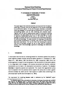
The goal of modelling is to develop a model that represents a particular system. A modeller often performs multiple tasks during the development of a model, such as obtaining knowledge about the system, implementing the model and disseminating the results. Moreover, modellers are typically part of a community and make use of the assets that the community has developed. An overview of all the aspects that are relevant to the development of a model are shown in Figure 1. Reality Community Assets Other Assets
Models
Tools
Formalisms
Systems Modeller Obtaining Legend Input/Output Required for Interacts with
Modelling
Disseminating
Model
Figure 1: An overview of the development of a model. The squares are representations and the ellipses denote tasks. The representations are inputs and outputs of tasks. For clarity reasons, not all the interactions are shown. Small circles represent tasks between items, while small squares refer to representations between tasks.
Models are typically developed in a formalism. Such formalisms are developed to suit the objectives of the community. Directly using a formalism is often considered impractical. As such, tools are developed to make the modelling process easier. Modellers can develop models in the formalism by using the tools. Communities are typically interested in particular kinds of systems. The members of the community can make models of these systems, but often also create other assets that describe these systems. These can include textual descriptions, visual depictions, and data sets based on observations. The developed models are not only based on the systems themselves, but typically also on these other community assets. There are three tasks that a modeller can perform that are relevant to the development of a model: obtaining, modelling and dissemination. In the obtain task, the modeller gathers information necessary to develop the model. As such, the system and the community assets are inputs for this task. The modeller can obtain information about the system by directly observing the system. Some modellers may already have knowledge about the system through years of examining such systems. The modeller is typically not the only one interested in the system. Within the community there are potentially others who have analysed such systems and developed assets that describe them. There might even be models available that represent the
2.2 what is modelling?
system. The analysis of these models and other assets allows the modeller to gain an understanding about the system. The models that have already been developed about the system are also useful in other ways than obtaining knowledge about the system. Existing models in the community might be sufficient to fulfil the goals of the modeller, which might eliminate the need to develop a model. Models that partially represent the system of interest can also provide insight in how parts of the system can me modelled. Moreover, parts of the model might be suitable to reuse in the modelling task. Gaining expertise in using formalisms and tools is essential in order to create a model in the correct way. Information about the formalism can be obtained in many ways. Documentation about the formalism can explain the primitives that it contains, their meaning and their intended use. Example models and models made by the community can explain the formalism through their use. Visualisations of models in tools can also contribute to a modeller’s understanding of the formalism. The availability of tools for particular formalisms can be a reason to choose a certain formalism. Moreover, expertise with the tool is required to be able to use the tool effectively. Such skills can be gained through documentation, videos showing models being built in the tool and by working through tutorials. The second task that has to be performed in the development of a model is the modelling task in which the modeller uses the tools to implement the model in the formalism. The inputs for this task are potentially all the community assets and the knowledge that the modeller has obtained. In the modelling task the models and other assets can play a direct role. Parts of models can potentially be reused, while the use of other assets is diverse. For example, data can be used to determine whether a model corresponds with observations, calibrate the parameters of a model, or form the basis from which a model is inferred. Textual descriptions can potentially be used as a data source in models, while visual depictions might be incorporated in the visualisation of the model. The final task in developing a model is dissemination. This is not just the sharing of the model with the community, but also any other results that have been established in the modelling process. Such results can include documentation explaining the model, new knowledge about the system, and knowledge about how a formalism should be used to represent particular aspects of systems. The three tasks relevant to developing a model are actually more integrated than described so far. The modelling task not just makes use of the information gained in the obtain task, but can itself result in acquiring knowledge. The reason is that during modelling the modeller makes his knowledge about the system explicit in the formalism. The decisions on how to model parts of the system in the formalism can change the modellers understanding of the system. Noticing that modelling a part of the system in a particular way does not work may have the same effect. Finally seeing inconsistencies or unwanted implications of the model (potentially inferred via automated reasoning) can cause the modeller to change his conceptualisation of the system. Such changes in knowledge may inspire revisions in the model that is being developed. Working on the dissemination task may have similar consequences. Describing the model and its implications in a text can cause the modeller to reconsider the model and his knowledge about the system.
11
12
difficulties in conceptual modelling
2.3
what is a model?
Many of the modelling difficulties reside in the modelling task. Three questions are addressed to provide a better understanding of modelling. What is a model? What can be modelled? How are things represented in models? Answering these questions provides insight in the relationship between the model, the formalism and the system it represents and what actually happens in the modelling task. A model can be thought of as a set of representations. A representation has three properties: 1. A representation is a depiction of something else, called the referent. As such, there is a mapping between the representation and the referent. 2. A representation is an abstraction of the referent. This means that only some properties of the referent, which are considered useful for a particular purpose, are reflected in the representation. As such, a representation can be considered as simplification of the referent. 3. The modelled properties of the referent are depicted as distinct primitives in the chosen formalism. For example, the length of a room is depicted as the length of a line in a floor plan. Whether something is to be considered a representation is partially subjective, as someone has to accept that the representation is a depiction of the referent. For example, the first line of a floor plan of an apartment is a representation of the length of the room for the author, but may simply be a line for someone else seeing it. Having established what models and representations are, the focus can shift to what can be modelled. To this end, it is relevant to distinguish systems in reality, ideas about those systems in someone’s mind, and models as artefacts. Consider a system in reality that someone wants to model. The modeller can experience this system through sensory perception and form ideas about that system. These ideas can be considered a model of the system consisting of a set of internal mental representations that depict referents in the system.1 These mental representations can be considered to directly depict the system. Consider now a modeller who develops a model based on the information obtained by observing the system. Strictly speaking, this model is not a direct representation of the system in reality. Instead it can be considered to be a representation of the ideas that the modeller has about the system. Another important aspect in what can be modelled is the amount of referents that a single representation refers to. A representation can refer to a single referent, such as the design of a single unique house. Such a representation can be called a specific representation. However, a single representation can also refer to multiple referents. For example, a design for a set of houses. Representations which apply to many referents are called generic representations. Similarly, a model that consists of generic representations can be called a generic model, and a model with only specific representations can be called a specific model. 1 Note that in the rest of this thesis, the word model is reserved for models represented in a formalism. To refer to representations in someone’s mind the word mental representation is used. Moreover, the nature of these internal mental representations is outside of the scope of this thesis.
2.4 conceptual modelling for science and education
Having described what a model is and what can be modelled, the remaining question is what primitives can be used to represent referents. Since formalisms are almost always of a different nature than that which is represented, the properties of the referent have to be modelled as features in the formalism. The choice concerning what a referent is modelled as should be made in such a way that the properties of the referent correspond with the properties of the feature it is represented as. In the room example above, the referent is the length of the room and the feature in the formalism is the length of the line in the floor plan. In summary, the task of modelling can be considered as consisting of choosing referents in a system, choosing what properties of those referents are important to capture, choosing a formalism, and representing the properties of the referent as features in the formalism. The result of this activity is a model that represents the chosen system. 2.4
conceptual modelling for science and education
This thesis addresses difficulties with conceptual modelling as experienced by science researchers and students. To appreciate the particular complications these modellers encounter, their goals, the role of modelling in their activities, and the formalisms that they use are described. Particularly, understanding the nature of these formalisms, referred to as articulate models (Bredeweg and Winkels, 1998; Forbus et al., 1999), provides insight into the intricateness of modelling for science and education. The goal of science researchers is the advancement of science. This can be considered the organisation, development and testing of scientific theories about phenomena through application of the scientific method.2 Phenomena can be considered the behaviour of systems (von Bertalanffy, 1950). As such, a scientific theory has to explain observations of systems and predict the behaviour of similar systems (i.e. future observations). The desired end products for scientists are publications describing theories, models, data sets, and new formalisms and tools (i.e. the community assets described in Section 2.2). The main goal of science education is students acquiring a scientific understanding of systems (Eurydice, 2006). Such an understanding can be considered knowing how systems behave and being able to explain why they do so. This requires students learning scientific theories and the skills to apply this knowledge to systems. A second goal within science education is students learning the scientific method in order to understand why scientific theories are considered to be correct. Scientific modelling can play an important role in both science and science education. Within science, a model can be considered a representation of how a scientific theory applies to a particular system (Frigg and Hartmann, 2009). Simulating the model allows the behaviour of the system to be predicted. Models can be useful in multiple ways. The simulations of a systems allows theories to be tested against observations. Moreover, the simulations allow future observations of particular systems to be predicted. Finally, the process of modelling can help a scientist formulate theories more precisely as it requires making ideas explicit.
2 Typically, the explanations that scientists propose for observations are called conjectures. A conjecture is called a scientific theory if enough supporting evidence (in the form of observations) and no contrary evidence is found (Popper, 2003).
13
14
difficulties in conceptual modelling
The use of models in science education is less well-established than in science. An innovative application is students learning about a particular domain by developing, testing and revising models. This goes beyond allowing students to run simulations and change parameters. It requires students to express and externalise their thinking about systems and test parts of their theories which can advance their knowledge (Schwarz and White, 2005). The simulations allow students to be confronted with the consequences of their ideas. Through modelling and simulation, students can learn scientific theories, how they apply to particular systems and how such systems behave. In short, modelling allows students to acquire an understanding of systems. Although the goals of science and education differ, explanations can be considered central to both enterprises. An explanation can be considered the answer to a why question, and is typically thought of in terms of causation (Mayes, 2001). As such, an ideal scientific model should provide both a simulation of the behaviour of a system and also be able to provide an explanation about why this behaviour is produced. However, traditional numerical models tend not to produce explanations of the behaviours that they predict. Moreover, they leave the assumptions made by the modeller during construction implicit (Forbus and Falkenhainer, 1990). The explanatory power of scientific models is especially an issue when explanations and dialogue need to be generated automatically, such as in an interactive learning environment (Brown et al., 1982; Hollan et al., 1984). To be able to provide explanations and have a dialogue with students within such a context, the modelling formalism used to construct models should be articulate (Bredeweg and Winkels, 1998; Forbus et al., 1999). That is, there should be sufficient conceptual distinctions in the modelling vocabulary that the formalism provides. Articulate models allow an explanation to be generated about a phenomenon using the knowledge in the model. That is, the model explicitly represents all the knowledge that is required for someone to understand phenomena, which is beneficial for both science and science education. Articulate models are a form of conceptual models and can have a varying degree of articulateness. Their conceptual nature is essential as both beginners and experts often prefer reasoning about systems in conceptual terms (Brown et al., 1982). As such, these conceptual terms should be explicitly represented. Moreover, in order to provide an adequate explanation of a system, articulate models require the representation of several kinds of knowledge. Consequently, the formalism that is used to develop such models should fulfil particular requirements. Being able to represent each of the following aspects of systems contributes to a formalisms suitability to develop articulate models. system structure A scientific theory typically applies only to a particular class of systems. A representation of the physical structure of the system is required to explain the scope of systems to which the theory is applicable. For example, the Lotka-Volterra equations only apply if there are two (or more) populations in which one is preying on the other. Moreover, the physical structure of a system can have significant impact on the behaviour that a system exhibits (Forbus et al., 1999). Therefore, to be able to explain the behaviour of such systems, the structure has to be explicitly represented. Such representations also makes explanations easier to understand, as quantities are explicitly associated to parts of the system.
2.5 formalisms
causal representation of processes Central to scientific theories are processes, which are the mechanisms that cause change within a system. The representation of processes in models allows simulations. However, an articulate model not only describes how a system changes, but should also be able to explain why such changes occur. Such explanations are causal in nature (Mayes, 2001). Consequently, to explain the behaviour of a system, an explicit representation of processes involved as causal mechanisms is essential. quantities and time Models and especially their simulations tend to represent the changes of quantities over time numerically. As mentioned previously, such a representation is not well-suited for the generation of explanations (Forbus and Falkenhainer, 1990). Minor changes in a quantity are typically irrelevant for an explanation and going through each of the values of quantities is not helpful. Those changes in the behaviour of systems that are interesting tend to be caused by a quantity reaching a particular threshold value (such as boiling point). Consequently, for purposes of explanation, a qualitative (conceptual) representation of quantity values, which captures such landmarks explicitly, is required. Such a representation of quantities has an important consequence on the representation of time. For purposes of explanation, the periods of time in which the system exhibits no relevant changes should be grouped together, so that only conceptually interesting changes in the system remain. generic and case-specific knowledge Articulate models have to be able to explain how a particular system will behave based on general knowledge about the class of systems to which the system belongs. This ability requires that the representation distinguishes between the information about the particular system that is represented, and the general knowledge that applies to that system. By using this distinction, explanations can distinguish between the knowledge that is particular for the system and the knowledge that is more generally applicable. assumptions Assumptions are an important reason why a model shows a particular behaviour and are therefore essential in the generation of explanations (Forbus and Falkenhainer, 1991). Two typical categories of assumptions that are distinguished are simplifying assumptions and operating assumptions. Simplifying assumptions inform about the perspective and granularity that have been chosen in the modelling of the system, but also what kind of approximations have been built into the model. Operating assumptions are used to control the simulations with the purpose to focus on particular behaviours. As a result of the different kinds of knowledge that are explicitly represented in articulate models, the formalisms that are used to create such models are intrinsically intricate. The difficulties for modellers that potentially follow from this are discussed in the next sections. 2.5
formalisms
The formalism chosen to represent a particular system largely determines the difficulty of developing a model. In order to become proficient, the modeller has to learn both the formalism and modelling using the formalism
15
16
difficulties in conceptual modelling
(as part of the obtain and modelling tasks , Section 2.2). The properties of formalisms can cause a number of difficulties in the development of models. The main issues, discussed below, are attributing meaning to formalism terms that is inconsistent with the allowed inferences, attributing meaning to formalism terms that is inconsistent with the meaning attributed by the community, developing syntactically correct models, and deriving the allowed inferences from a model. 2.5.1
Attributing meaning inconsistent with inferences to formalism terms
The meaning of formalism terms can be difficult to learn. The terms constitute a meta-vocabulary with which domain concepts can be expressed. Conceptual modelling formalisms, such as those used to develop articulate models, commit more to a particular perspective of reality than more generic languages. For example, concept maps distinguish only concepts and relations (Novak and Gowin, 1984), while qualitative modelling formalisms defines terms for entities, quantities, causal relations, and others (Bredeweg and Salles, 2009b). As a result of making more ontological commitments, the meaning of terms in conceptual modelling formalisms can seem close to a modellers everyday understanding of the concept. However, the high level concepts that make up the vocabulary of the formalism may not directly match with preconceptions and common sense notions of modellers. For example, humans have an evolved inherent model of causality that emerges in early childhood (Pinker, 2007). This model seems to be different from the notions of causality as used in the Garp3 QR formalism, which distinguishes direct causation and indirect causation (Bredeweg et al., 2006a, 2009) (Section 3.3.3).3 This mismatch might be one of the causes that makes these formalism terms difficult to learn. One particular modelling difficulty arises when there is a mismatch between the attributed meaning and the meaning that is captured in the inferences of the formalism. In such a case, the modeller will have difficulty understanding why particular inferences can be made. Moreover, dealing with such preconceptions can be difficult.4 This issue occurs less for terms in more abstract formalisms, as they typically do not evoke such common-sense interpretations. There are several additional issues that make learning the meaning of terms difficult. When more terms are involved in inference, it takes more effort to understand the role of each of these terms. If the number of reasoning steps that the inferences require is larger, it is more likely that modellers make mistakes deriving conclusions. If there are a number of terms that are seemingly similar, such as union and intersection in set theory or different forms of causality in qualitative models, it is more likely that modellers will confuse them. Finally, people tend to be trained in mathematics from a young age, but are typically not introduced to any form of conceptual modelling. Consequently, conceptual modelling formalisms are unusual for most modellers and therefore difficult for them to learn. The issues with learning the meaning of the terms mentioned above make supporting their acquisition an important and challenging task. To allow hands-on learning of the meaning of the terms, and to provide immediate 3 Pinker
notes that this inherent model differs from Newtonian physics (Pinker, 2007). of Behavioral and Social Sciences and Education, National Research Council of the National Academies, 2005). 4 (Division
2.5 formalisms
feedback on misconceptions, the means of learning should be integrated in the modelling process. The question to be answered is: How can tools support the acquisition of term meaning as part of model development? 2.5.2
Attributing meaning to terms inconsistent with the community
The meaning of terms in conceptual modelling languages is determined by the inferences that the terms allow, and the meaning that is attributed to the terms by the community. This makes conceptual modelling formalisms different from logic or mathematics in which the term meaning can be considered to be fully determined by the inferences that they allow. Consequently, a potential difficulty when learning a conceptual modelling formalism is that the meaning attributed to terms by the modeller (Section 2.5.1) can differ from the meaning that the community ascribes to them. Consequently, when the model is disseminated, the community can disagree with how terms are used. For example, a relationship represented as a concept in a concept map (Novak and Gowin, 1984) can be considered incorrect by the community. The inconsistency between modeller attributed meaning and community attributed meaning is partially solved by conceptual modelling formalisms that allow for inferences. The meaning that is attributed by the community must be consistent with the inferences that a term allows. As a result of allowing inferences, there is an enforced minimum consensus of the meaning of the terms. This feature of formalisms is an important feature that allows for clear communication. As such, as long as a modeller uses terms consistent with the inferences that they allow, this issue is partially solved. In spite of inferences, it is still possible for the meaning attributed by the modeller to be different from the meaning that the community associates with a term. Consider configurations in the Garp3 QR formalism (Section 3.3.1), which are meant to represent structural (mereological, spatial and process) relations. Modellers sometimes use these ingredients to represent causal or subsumption relations (Section 5.3.3). Such use of configurations does not prevent correct simulations to be generated. As such, the meaning attributed to configurations does not conflict with the inferences they allow (Section 2.5.1). However, the meaning does conflict with the meaning that is attributed to configurations by the community. How can the modeller be supported to use formalisms terms in a way that is consistent with their usage within the community? As this disagreement pertains to the non-formalised aspects of terms, this issue is difficult to resolve. Moreover, the means of support should detect discrepancies in term use early in the modelling process so that the consequences of amending the model are minimal. 2.5.3
Developing syntactically correct models
Within a formalism, the way formalism terms can be combined is determined by the syntax. Syntactically correct models are said to be well-formed. Accidentally creating syntactically incorrect models can result in the wrong meaning being associated to such models and wrong inferences being drawn. This is especially an issue in articulate models, as they distinguish many terms, and these different types of knowledge can only be combined in particular ways. As a result, relatively few of the combinations of terms result
17
18
difficulties in conceptual modelling
in syntactically correct models. Syntactically incorrect models can be prevented by tools (Section 2.6). 2.5.4
Deriving allowed inferences from a model
The inferences that are allowed by a formalism can be intricate and result in a multitude of conclusions. As a result, doing the inferences by hand can become error-prone and time-consuming. Articulate modelling formalisms can be particularly affected by a large number of conclusions for two reasons. Firstly, some articulate models can generate all the possible behaviour of a system, which is called a total envisionment (Forbus, 2008). Such a simulation generates all the conceptually distinct states that the system can be in and all the possible transitions between them. An envisionment consists of all the possible evolutions of the system from each possible begin state, while a typical simulation only shows one such behaviour. Secondly, compared to numerical simulations that typically predict exactly how quantities will change numerically, articulate models describe the quantities on a conceptual level. This abstraction tends to be at the cost of information that determines which behaviour of a system will occur, resulting in ambiguity that causes additional results (Forbus, 2008). For example, due to the difference between the natality and mortality rates of a population being unknown, the population size could either increase, decrease or remain steady. Each of these behaviours would be shown in the simulation. These difficulties of deriving inference by hand can be resolved by using tools that allow for automated reasoning (Section 2.6). 2.6
tools
The development of a model in a particular formalism is typically done through a tool (Figure 1). Tools can solve important difficulties, such as preventing syntactically incorrect models and performing automatic reasoning. Such reasoning makes implicit knowledge explicit and detects inconsistencies in models. Consequently, it allows the modeller to focus more on modelling instead of determining the logical consequences of a model manually. However, through use of a tool, other issues emerge. These can occur while learning to use the tool, modelling using the tool, trying to understand the simulations, and while refining the model to improve the simulation results. 2.6.1
Learning the tool
In order to develop models using a tool, the modeller has to learn the overall interface, the graphics that are used to represent particular terms, and the interactions that are necessary to manipulate the terms. Learning the overall interface depends mostly on the number of features that the software supports. Learning the graphics and associating them to the correct terms tends to be more difficult. Conceptual modelling languages are typically designed to be domain-independent. As a result, the graphics designed to represent the terms are typically of an abstract nature which makes them difficult to learn. Finally, the modeller has to learn to manipulate the terms, such as adding, changing and deleting them. Typically, the manipulations that can be made depend on the number of terms in the formalism. A higher number of manipulations increases the possibility of choosing the wrong
2.6 tools
manipulation, as each manipulation of a term often becomes a button or menu item. Developing means of support that allows a tool to be learned more efficient is an important undertaking. How can tools be developed in such a way that learning to use them takes less effort? 2.6.2
Modelling using the tool
In conceptual modelling formalisms, there are many possible combinations of terms and few valid combinations (Section 2.5). Tools can play a role in preventing modellers from combining terms in syntactically incorrect ways (such as in Garp3 (Bredeweg et al., 2009) and Protégé (Knublauch et al., 2004)). However, this still leaves the issue of the finding the possible valid combinations of terms to the modeller. This causes two issues for the modeller in the modelling task. Firstly, the modeller can try to develop a representation by developing an illegal combination of terms. As this is prevented by the tool, the modeller can become stuck. The issue is that the modeller is unaware of the correct combination of terms that would resolve his modelling problem. Secondly, modellers can be unaware of particular combinations of terms. Consequently, there is a need to develop the means of support that makes modellers aware of term combinations that solve particular modelling solutions. 2.6.3
Understanding the simulation results
There are two main issues that modellers have to deal with when trying to understand simulation results: (1) understanding the conclusions themselves and (2) understanding why those conclusions have been drawn. As mentioned in Section 2.5, a large number of conclusions can be drawn from articulate models. Furthermore, the conclusions typically comprise multiple representations that represent different kinds of knowledge, and consist of large sets of different terms. Consequently, there is a large amount of information to process when analysing a simulation and deciding whether the results are desirable. To understand why particular simulation results are present, the way these facts have been derived is important. However, it is possible that the automated reasoning hides the proofs that have lead to conclusions. As a result, it can be difficult for a modeller to understand why a particular conclusion is valid. Even when the proofs are made visible to the modeller, they can be intricate as a result of being long and requiring non-trivial application of rules. Furthermore, many terms can interact to produce unexpected results. Finally, inference rules can be implicit, which makes it difficult for modellers to understand the validity of conclusions and proofs. In short, it can be difficult for modellers to understand simulation results. As a consequence of the issues above, modellers require means of support. How can modellers be supported in understanding simulation results? 2.6.4
Correcting the simulation results
Once a modeller has managed to understand the simulation results, there are potentially two issues to contend with: (1) removing unwanted simulation results and (2) adapting the model so that missing desired behaviour is generated. In articulate models, which can potentially generate many simu-
19
20
difficulties in conceptual modelling
lation results (Section 2.5), the chance that part of the conclusions are considered spurious is large. Consequently, modellers require an understanding of why the results are generated and how the behaviour can be constrained. Adapting a model so that it generates particular missing behaviour is typically more difficult. There can be multiple reasons why particular conclusions are not drawn, but the most important cause are inconsistencies. These are the result of a set of terms or axioms being contradictory. Inconsistencies are typically difficult to resolve by modellers. It requires them to determine which combination of terms in the model results in the inconsistency and determine which of them has to be changed in order to resolve it. Such issues become worse if inconsistencies require intricate proofs to derive. In addition to the representations in the model itself, there can be constraints on inferences that are part of the formalism. This increases the chance of inconsistencies. When inferences are done automatically, determining the causes can be difficult due to such constraints being implicit. Correcting simulation results is a challenging task in the modelling process. There is a strong desire for a means of support from modellers. Therefore, the problem to resolve is developing the means by which modellers are empowered to overcome the above obstacles and refine their model so that their desired behaviour is generated. 2.7
scientists and the scientific community
Much of science depends on building upon earlier work and collaboration. Consequently, important activities are obtaining relevant related research and disseminating achieved results within the community (Section 2.2). In addition to the problems with formalisms and tools discussed previously (Sections 2.5 and 2.6), there are several issues that make model development challenging for scientists. These relate particularly to the interaction between modellers and their community. Below four key issues are brought forward: terminological alignment, access to existing models, automated model comparison, and (partial) model re-use. 2.7.1
Terminological alignment
Within science, clear communication is an important goal. In order to attain this objective, research communities require the collaborative establishment and consistent use of terminology in models (Lewis, 2004; Tudorache et al., 2008). Using the scientific nomenclature is important as it allows the community to understand the model, compare it to other results, and assess its significance for ongoing research. Moreover, it allows the scientist to position their research with respect to the work present within the community. For scientists it can be difficult to adhere to an accepted scientific vocabulary during the development of a model. The focus tends to be on creating an adequate representation of a model, and aligning with the community may appear as extra burden on an already time consuming and difficult task. As such, the issue of divergent terminology may only become apparent during later stages of the development or even as late as during dissemination. At this point changing the terminology can have significant impact due to differing conceptualisations of the system. Note that the issue of using the correct terminology is even more difficult to resolve when building interdisciplinary models. Assets in communities tend to use reasonably consistent
2.7 scientists and the scientific community
terminology internally, but terms are potentially used in different ways in different communities (known as the silo effect (Ceusters and Smith, 2010)). Consequently, there is a desire for a solution that allows the consistent use of terminology to be established during the modelling process. For scientists, it is not enough to use the terminology that has already been established within a community. Part of research is the invention of new conceptualisations and terminology that better capture particular aspects of systems. A solution that supports scientists in using the correct terminology should also allow suggestions for new terminology to be proposed to the community. The quest thus is to seamlessly interleave the assessment of proper use of vocabulary within the modelling task as much as possible. 2.7.2
Access to existing models
In addition to using the appropriate terminology, scientists need to compare their modelling efforts with models made by others in the community. It is necessary to assess and understand the potential differences with earlier work and to clearly articulate novel contributions. However, access to scientific models is not widely available. Scientists tend not to make their models publicly available and only share them upon request. Typically, scientists get to know about a model indirectly via a publication, even though efforts are undertaken to share models more efficiently (De Roure et al., 2009; Noy and d’Aquin, 2011). There is need within the scientific community to make models available and to be able to search for them. 2.7.3
Automated model comparison
When comparing their developing model with models from the community, scientists tend to be particularly interested in the aspects of a system that are modelled differently, what important aspects should still be incorporated, and what parts of the model can be considered unique. However, the manual comparison of a developing model with other models can be a labour-intensive task. As such, a tool that allows such comparison to be made automatically would greatly contribute to the work of scientists. 2.7.4
Model re-use
In order for scientists to advance science, they have to built upon earlier work. When developing scientific models, this typically requires scientists to reimplement parts of existing models. This in itself does not contribute to the researchers goals (assuming that the earlier work does not need replication). Researchers would prefer to use the time necessary to do such redevelopment on developing aspects of the model that are innovative. The development of a tool that would allow scientists to reuse parts of existing models would be an important contribution that resolves these issues. The main difficulty to overcome in the development of such tools is integrating different models in a meaningful way.
21
22
difficulties in conceptual modelling
2.8
education
Science education goals include important characteristics such as students learning domain theories (and retaining them in the long term), gaining the ability to apply theories in new settings, being motivated towards learning, and students developing higher order thinking skills (Bloom, 1984). Pedagogical approaches based on constructivism have become popular means to attain these goals. The theory of constructivism posits that knowledge is gained through a process of active construction (Piaget, 1970). This thesis focusses in part on Learning by Modelling (LbM), a form of active learning (Bonwell and Eison, 1991) in the constructivist tradition as students are "involved in a process of creating, testing, revising, and using externalized scientific models that may represent their own internalized mental models" (Schwarz and White, 2005). Although LbM approach can still be understood in terms of the tasks described in Section 2.2, and the issues with learning the formalism and tools still apply (Sections 2.5 and 2.6), its use in education has important unique consequences. Modelling is by its nature an autonomous activity, as students are given the freedom and responsibility to make modelling decisions. Such decisions include deciding in which order (and how) particular aspects of a system are represented. As a consequence, there can be a large variation in the developed models, while at the same time norms to evaluate specific results are less easily available or even missing. How to provide valuable support for students in this setting? Below the key issues relevant to this question are presented: Learning and using the appropriate domain terminology, getting feedback on a specific modelling result, deciding upon the next challenge for LbM, and finally encouraging good modelling practices while working towards the construction of a particular phenomena-explaining model. 2.8.1
Learning and using the domain terminology
An important goal in learning about a domain is using the correct terminology. The scientific nomenclature should be considered normative in an educational context. Consequently, students should be encouraged to use this terminology in their models. However, simply providing students the vocabulary that they should use does not seem to be an appropriate solution, as it would be in conflict with the idea of learners being in control and actively acquiring and constructing their knowledge. Consequently, an important issue to be resolved is how students should be supported in learning and using the correct domain terminology while preserving the autonomy and freedom of the LbM approach. 2.8.2
Getting feedback on modelling results
During modelling activities, students often want feedback relating to the correctness of their models. Such feedback can consist of pointing out missing (or superfluous) aspects of the system and indicating that parts of the system are represented using the wrong terms in the formalism. However, teachers can become a scarce resource in a LbM context, as supporting students can be difficult and time-consuming. Consequently, multiple teachers can be required to properly support all students.
2.8 education
The intrinsic difficulty of providing feedback is mainly caused by students being autonomous and making their own modelling choices. As a result, the models can be vastly different among students (even within a single course). A teacher requires time to analyse the model in order to be able to give adequate feedback. As a result of the difficulty of providing feedback in LbM settings, there is a challenge to develop a method that would allow the automatic generation of such feedback. This would ensure that students always have access to support. However, such a solution has to deal with the diversity of built models and the potential lack of norm models. 2.8.3
Deciding the next modelling challenge
After finishing modelling a particular aspect of a system, students may not know which problem in the curriculum to address next. Such students require guidance from a teacher in order to proceed. The issues supporting students, such as a diversity of models, still apply. However, there are additional difficulties to suggesting a new modelling challenge that make the situation worse. The possible options strongly depend on what the modeller has implemented so far. Moreover, the new problem should be difficult enough to be educationally valuable, while still being feasible enough for the student to complete the task. There are potentially many aspects of systems that could be modelled fulfilling these requirements. This makes determining good modelling opportunities difficult. Ideally, the student would be able to take control and autonomously make the choice about what to model next. Inventing an automated solution that addresses the above issues would strongly contribute to the use of LbM in classrooms. Such an instrument should allow a curriculum to be set by a teacher and offer dynamic guidance to the student, while leaving the path through the curriculum free to the student. A more open-ended form of guidance would remove the restriction of a curriculum and make use of the assets available in the community to dynamically generate modelling problems (Section 2.2). 2.8.4
Encouraging good modelling practices
Beginning modellers often encounter difficulties due to using non-optimal modelling practices. This is an issue for both scientists and students, as it may require reversing earlier modelling decisions and loosing time redoing modelling work as a result. However, in an educational setting the students might lack the skills to identify that their modelling practices cause problems. In such cases, interventions are required. Non-optimal modelling practices include using modelling strategies that cause difficulties, making poor modelling decisions, and using inelegant solutions to have models produce the desired behaviour. To address this issue, metamodelling knowledge (Schwarz and White, 2005) should become part of the curriculum in LbM approaches. However, such knowledge is not readily available to students and educators (Eurydice, 2006). As such, there is a need for a catalogue of frequently occurring non-optimal modelling strategies and modelling choices, more effective strategies, and guidelines on how better modelling decisions can be taken.
23
24
difficulties in conceptual modelling
2.9
conclusions
The development of articulate models plays an important role in both science and education. Within science, such models represents how scientific theories apply to a particular system and can explain why it exhibits particular behaviour. Within education, a learning by modelling approach allows students to refine their ideas about systems. However, the development of such models is hampered by issues with the formalism and the tools. Moreover, means of support are missing to handle the particular requirements in scientific and educational settings. With regard to the formalism and the tools, the important obstacles are learning the meaning of the terms, learning to use the tools and understanding the simulation results. These issues hamper the adoption of articulate models in science. Within educational contexts, articulate modelling is resultantly infeasible as these problems make the practice too difficult and timeconsuming for young students. Additional issues during model development are suboptimal modelling practices and the difficulty of troubleshooting simulations. Means of support are required to resolve these difficulties. Within science, there is the issue of employing the terminology that is conventionally used within the community. An additional complication is that scientists can invent new terminology that can be adopted. These practices have to be supported in the modelling process in order for models to be understandable and to prevent redoing modelling work to refine terminology late in (or after) model development. Another issue within the scientific community is the lack of access to models, and consequently the problems of comparing results and reusing parts of models. These issues have to be supported in tools to make modelling have more impact within science. Students have a number of specific difficulties when developing models. As part of their education, they should be supported in using the domain vocabulary as part of the modelling process. Moreover, they tend to require feedback on the correctness of their models and are often blocked when having to choose a new curriculum problem to address. Automated solutions to these issues are needed, as teachers can become a scarce resource in the LbM approach as a result of the time required to analyse the diverse models that students construct.
3
W H AT I S Q U A L I TAT I V E R E A S O N I N G ?
Broadly speaking, the research in qualitative physics is aimed at developing representation and reasoning techniques that will enable a program to reason about the behavior of physical systems, without the kind of precise quantitative information needed by conventional analysis techniques such as numerical simulators. (. . . ) Observing pouring rain and a river’s steadily rising water level is sufficient to make a prudent person take measures against possible flooding without knowing the exact water level, the rate of change, or the time the river might flood. — Yumi Iwasaki (Iwasaki, 1997) Qualitative modeling concerns representation and reasoning about continuous aspects of entities and systems in a symbolic, human-like manner. — Kenneth D. Forbus (Forbus, 2008) Qualitative simulation predicts the set of possible behaviors consistent with a qualitative differential equation model of the world. Its value comes from the ability to express natural types of incomplete knowledge of the world, and the ability to derive a provably complete set of possible behaviors in spite of the incompleteness of the model. — Benjamin Kuipers (Kuipers, 2001) Qualitative Reasoning (QR) is an area of artificial intelligence that researches the conceptual representation of systems (Forbus, 2008).1 QR particularly focusses on representing the continuous properties of systems, such as quantities, space and time, emphasizing qualitative (conceptually relevant) distinctions. Modelling is central to QR. First, as a field of Knowledge Representation (KR) (van Harmelen et al., 2008), QR focusses on the development of representations that allow for reasoning about (physical) systems. This enterprise results in QR formalisms. Second, domain experts that use QR formalisms as an instrument contribute to the QR field by investigating how particular domain aspects should be modelled, and what kinds of representations and reasoning are required to accurately explain features of phenomena. Qualitative modelling can be considered a form of conceptual modelling.2 The concepts that a conceptual modelling language distinguishes through its primitives are its ontological commitments. These ontological commitments determine the language’s inherent perspective on what constitutes
1 Due to its name, qualitative reasoning is easily associated with qualitative research, such as ethnographic or participant observation types of research, which is inherently subjective and does not employ mathematical models. The reader is invited to forget these associations, as qualitative reasoning is unrelated to these fields. 2 Throughout most this thesis, constructing QR models is presented as a form of conceptual modelling, while understating QR as a form of KR. This is done to keep the text understandable for non-computer scientists who are interested in QR. Readers interested in QR from a KR perspective are suggested to read Appendix E.1 before reading the rest of the chapter. Afterwards, the rest of Appendix E can be consulted for an explanation of the QR representations in terms of KR.
25
26
what is qualitative reasoning?
knowledge, and via knowledge, how reality should be perceived. Particularly, QR views the world as systems that consist of entities, of which the continuous properties can be described by discrete values. This chapter focusses particularly on the QR implemented in the qualitative modelling and simulation tool Garp33 (Bredeweg et al., 2006a, 2009). The purpose, history and main applications of Garp3 are discussed in Section 3.1. Garp3 is based on established principles in the QR field on how systems should be represented. These principles are discussed in Section 3.2. The terms that Garp3 QR formalism provides to develop models are discussed in Section 3.3. An application of the formalism is presented in Section 3.4, which explains an osmosis model and shows the Garp3 visualisations of the model parts. The workings of the Garp3 reasoning engine, which predicts the behaviour of a modelled system is discussed in Section 3.5. Section 3.6 shows the visualisation of the simulated behaviour of the osmosis model and explains how the reasoning engine derives the results. Section 3.7 concludes this chapter. 3.1
garp3: qualitative modelling and simulation workbench
Garp3 is a tool that allows the development and simulation of qualitative models (Bredeweg et al., 2006a, 2009). The QR formalism implemented in Garp3 allows the modelling of conceptual representations of systems and represents the processes that govern such systems as causal mechanisms. The representation allows the prediction of the behaviour of the system through simulation. Garp3 is the result of years of research and development. The reasoning engine in Garp3, is based on the original program Garp (Bredeweg, 1992). Garp was designed to unify three alternative approaches to QR (QPT (Forbus, 1984), Envision (de Kleer and Brown, 1984), and QSIM (Kuipers, 1989, 1986)). Further development of the Garp engine led to Garp2 (Linnebank, 2004). Garp3 was developed by integrating Garp2 with VisiGarp, which generates interactive diagrammatic visualisations of simulation results (Bouwer, 2005; Bouwer and Bredeweg, 2010), and the diagrammatic modelling tool Homer (Jellema, 2000). As part of the integration, the design of the interfaces and diagrams was unified and improved through the development of a visual vocabulary for each of the terms in the QR formalism (see Table 1) (Bertels, 2007). Further development of Garp3 resulted in improvements to the reasoning engine, multiple language support, a Sketch environment (Bredeweg et al., 2008; Liem et al., 2007a) and a table view visualisation of the state graph (Bouwer et al., 2007). Since Garp, the notable new features include: diagrammatic modelling Garp3 allows models to be developed as diagrams. Modellers are informed about possible manipulations through highlighted buttons and are prevented from developing syntactically incorrect models. interactive visualisation of systems’ behaviour Simulation results are presented as interactive diagrammatic representations. Different sorts of visualisations provide overview and access to different kinds of results (Section 3.6). 3 The
Garp3 tool, documentation and example models are available at:
http://www.Garp3.org
3.1 garp3: qualitative modelling and simulation workbench
exogenous quantity behaviour This feature allows the direct specification of the behaviour of a particular quantity (e.g., increasing and stopping at maximum value, oscillating or parabolic), which is useful to represent dynamics that plays a role but is not the main focus of a model (Bredeweg et al., 2007b). The agent term has been added to the formalism to represent such exogenous influences to the system. simulation tracer Understanding the simulation results can be difficult. As a means of support, a tracer has been added that allows a modeller to follow the reasoning steps made during simulation (Liem et al., 2007b). simulation preferences The modeller can control the inferences that the reasoning engine can make through the simulation preferences (Bredeweg and Linnebank, 2012) window. For example, the fastest path heuristic reduces ambiguity in the predictions by enforcing changes that can occur simultaneously to do so. This can result in smaller state graphs. improved reasoning Reasoning algorithms have been significantly improved since Garp: • Improved calculation of the net effect of multiple interacting causal relations using the notion of an equation balance (see Section 3.5.1). • When required, second- and third-order derivatives can be calculated for quantities. • Determining transitions has been improved, e.g., through a strict separation of immediate and non-immediate transitions (i.e. the epsilon-ordering rule (de Kleer and Brown, 1984) in Section 3.3.5). • Additional correspondence relations (e.g., inverse quantity correspondence) have been added to create flexibility in expressing that particular values of different quantities co-occur (see Section 3.3.5). • Inequality reasoning has been made more efficient by isolating equations into related sets (instead of reasoning with the full set of equations). Garp3 was developed in the NaturNet-Redime (NNR) project4,5 in an effort to make QR technology accessible to researchers who are not computer scientists. As part of NNR, domain experts formalized conceptual knowledge in Garp3, particularly focussing on river restoration ecology and sustainability issues (Cioaca et al., 2009; Dias et al., 2009; Nakova et al., 2009; Noble et al., 2009; Nuttle et al., 2009). The resulting models were used as education material (Nuttle and Bouwer, 2009), but also as argumentation tools in decision making processes with stakeholders (Salles and Bredeweg, 2009; Zitek et al., 2009). As a result of the efforts within NNR, qualitative modelling has become an established instrument within environmental science (Bredeweg et al., 2006c; Bredeweg and Salles, 2009b). Although Garp3 is mainly used in environmental science, its domain-independent nature also allows it to be used in other domains, e.g., to teach physics (AlvarezBravo et al., 2004) or chemistry (Salles et al., 2004). Furthermore, the NNR models about sustainability not only contained aspects from environmental 4 http://www.naturnet.org 5 http://hcs.science.uva.nl/projects/NNR/
27
28
what is qualitative reasoning?
science, but also from domains such as economy, sociology and political science. 3.2
qualitative reasoning principles
Garp3 is based on established principles in the QR community on how systems should be conceptually represented (Bredeweg and Struss, 2003; Bredeweg and Salles, 2009a,b; Forbus, 2008; Kuipers, 1989). These principles are discussed in the following sections. 3.2.1
Qualitativeness
The conceptual representation of quantities (i.e. the changeable properties of systems) requires them to be represented as meaningful qualitative values. That is, for each quantity, the particular values in which the system behaves differently have to be identified. An important concept in this regard is the notion of landmarks, which are the particular point values in which a system changes from one sort of behaviour to another. Consider the following examples of landmarks. The critical value of the concentration of oxygen in a river below which most species of fish will die. Or, the critical mass of uranium-235 above which a sustained nuclear fission chain reaction will occur. Given a set of landmarks for a quantity, its possible values can be represented as a quantity space. Such a quantity space consists of a set of discrete values in linear order: the landmarks, which are point values, and the interval values between them. Numerically, an interval value consists of all values between the landmarks. However, qualitatively this is considered a single value. A quantity space for the oxygen concentration in a river might be {0, lethal, critical, sustaining}, in which lethal and sustaining are interval values. Quantity spaces can be established in two ways. First, they can be the result of a modeller capturing a conceptual interpretation of a system in a QR model. As such, the modeller thinks about the landmarks that are relevant for a particular task. Consequently, the same quantity can be quantized differently in various models. For example, in a model about a steam engine, the boiling point of water is an important landmark of the temperature quantity. By contrast, in a model about water body stratification and mixing, the boiling point is irrelevant, but the freezing point is essential. Notice that in this approach to establishing quantity spaces, numerical values play no role. Second, quantity spaces can be built by quantizing the continuous values of quantities. As such, a quantity space can be seen as an abstraction of the possible numerical values of a quantity. 3.2.2
Conceptual representation of behaviour
Simulating QR models results in an explanatory prediction of the behaviour of the modelled system. The simulation results consist of qualitatively distinct states, which are complete descriptions of the system in a certain state of behaviour. Transitions represent how the system can evolve from one state to its successor state, resulting in a state graph of possible behaviours and their mutual ordering. Importantly, each state describes a unique conceptually relevant behaviour of the system. Consequently, each change in qualitative value, or inequality between quantities, results in a different state. As values
3.2 qualitative reasoning principles
of quantities are represented as either intervals or points, each state can represent either a period in time (with duration), or a particular moment. QR models can generate two types of predictions. The first, the attainable envisionment, starts with a description of the system in a particular state. The reasoning engine derives a state graph which describes how the system will evolve from this particular state. An attainable envisionment does not have to result in a single path from initial state to end state. Instead, ambiguity that results from the conceptual representation (Forbus, 2008) allows the simulator to consider all the possible ways the system might evolve. Consequently, there can be multiple end states and different behaviour paths. This feature distinguishes QR models from typical numerical simulations. The second type of prediction is the total envisionment. Such a simulation generates all the possible behaviours of a system. That is, it generates all the possible states that a system can be in and all possible transitions. As such, it shows how the system can evolve from each possible initial state. Logically, every attainable envisionment of a system is a subset of its total envisionment. 3.2.3
Processes and causality
Within the QR community, there are different notions of causality. • First, derived causality, which is called mythical causality by de Kleer and Brown, is the idea that causality is the result of interactions between the different components of a system (de Kleer and Brown, 1984). The physical structure of a system is determined by a set of components connected via input and output conduits. The causality is determined at runtime for a particular system by examining how a disturbance propagates through the system’s network of components.6 • Second, causal ordering is the idea that causal relations can be derived through the structural analysis of the equations that govern a particular system (Iwasaki and Simon, 1986). The causal order is determined by how variables depend on each other (with independent variables being considered to be exogenously determined). • Third, in Qualitative Process Theory (QPT) (Forbus, 1984) every change is caused either directly or indirectly by a process. A process can be defined as a mechanism that causes change within a system. Within QPT, causal relations are explicitly represented. Influence relations represent the direct causal effects of processes, while proportionalities propagate the changes caused by influences. • Finally, Garp3 introduces the notion of exogenous quantity behaviour (Section 3.1) which represents the causal effects from an action or process external to the system. Furthermore, Garp3 refines the notion of correspondence by defining directed and quantity space correspondences, thereby providing an augmented vocabulary to refine the effects of causal relations. 6 This approach sometimes requires reasoning via Reductio Ad Absurdum (RAA) in order to derive the value of a variable. That is, each possible value of a variable is tried and the inconsistent results are removed. Garp3 allows the same type of reasoning by setting certain simulation preferences. De Kleer and Brown (de Kleer and Brown, 1984) note about RAA: "Indirect proofs explain a consequence by showing that all alternative consequences do not happen, and thus cannot establish a simple relationship between a cause and its effect."
29
30
what is qualitative reasoning?
The Garp3 QR formalism integrates several of these approaches to causality. Component-oriented QR models can be created by explicitly modelling components with input and output conduits and connecting them. Inequality statements should be used instead of explicit causal relations. The derived causality can be determined by inspecting the simulation trace (Section 3.1). Garp3 also adopts the influence and proportionality relations from QPT, which allows causal relations to be explicitly represented. The notion exogenous quantity behaviour originates from Garp3 and is therefore also available. Garp3 does not support deriving causal explanations through causal ordering. Domain experts typically use Garp3 to develop process oriented models using influences and proportionalities. Such qualitative models allow domain theories about the processes that govern systems to be made explicit. That is, the modeller can represent the type of systems that the process applies to (i.e. which system structures, Section 3.2.4), under what conditions the process is active, and which quantities the process affects. In addition to processes, the effects of actions by agents on the system can also be modelled using causal relations. Since such agents are typically considered external to the system, their behaviour is often represented using exogeneous quantity behaviour (Section 3.1). The explicit representation of causal relations plays an important role in the prediction of systems’ behaviour. During simulation, the processes and agents that are active are determined based on the structural description of a system (and the made assumptions). The result is a (causal) dependency model which describes how the quantities in the system are interconnected. It is this dependency model that allows the prediction of how the behaviour of the system will evolve, and provides an explanation of why it has done so. 3.2.4
Compositional modelling: from structure to behaviour
It is possible to derive a conceptual representation of a system’s behaviour based on a set of qualitative differential equations (Kuipers, 1986, 1994) or a causal model (Forbus et al., 2005; Leelawong and Biswas, 2008). However, Garp3 and other QR formalisms (Forbus, 1984; Forbus and Falkenhainer, 1991) allow domain theories to be decomposed and represented into different models parts. The reasoning engine in Garp3 allows the causal model of the system to be derived from these model parts. This compositional approach allows model parts to be reused within a model, such as re-occurring structures in a system, and makes the model easier to understand by being organised in smaller conceptually grouped units. To allow the reasoning engine to automatically assemble a causal model that applies to a system, the representation in a QR model has to distinguish between the physical structure of the system and its behaviour aspects. The (physical) structure of the system describes what the system is, and can be considered to remain unchanged (for purposes of the model). Specifically, the structure can be said to define the system. The behaviour of the system describes the aspects of the system that can change over time. The representation of a process (or action) consists of both these components. The (generic) structural description indicates in which (parts of) systems the process is active, and the behavioural description represents the particular causal relations that constitute the particular process. In short, based on a structural description of the system, the reasoning engine can determine
3.3 model ingredients
which behavioural ingredients, such as causal relations, apply to the system and derive the causal model. The causal model can then be used to predict successor states. An important principle in the representation of systems and theories as model parts is the no-function-in-structure (de Kleer and Brown, 1984), which states that laws that govern part of a system cannot make assumptions about the behaviour of the whole system. For example, stating that if the faucet in the kitchen is open, water will flow, breaks the no-function-in-structure principle. It makes the assumption that there is water under pressure inside the faucet, which is not the case if, for example, the main water valve is closed. In practice, making assumptions about the functioning of a full system is unavoidable. However, such assumptions should be made explicit in models as class-wide assumptions (de Kleer and Brown, 1984). 3.2.5
Assumptions and perspectives
In addition to the physical structure and behaviour of a system, assumptions also play an important role in understanding the behaviour of the system. Typically, modellers make assumptions during the development of a model, such as simplifying and operating assumptions (Forbus and Falkenhainer, 1991) and the class-wide assumptions mentioned above. An approximation assumption, such as resistance being assumed to be 0, has important consequences on the derived behaviour of the system. Consequently, these assumptions have to be made explicit in a model. Perspectives also play an important role in qualitative models, and can be seen as a way of conceptualising a system to achieve a particular goal, such as answering specific questions (Salles and Bredeweg, 2007). Perspectives are a form of assumptions, as they allow simulations to be run while focussing only on relevant properties, while ignoring those that are considered irrelevant. For example, perspectives allow simulations to focus on the economical aspects of a system, while ignoring the social aspects. Perspectives can be used to keep simulations manageable by not simulating all aspects of a system simultaneously. As a result of implementing the QR principles explained in these sections, the Garp3 QR formalism makes sufficient distinctions to explain system behaviour. As such, the formalism can be considered articulate (Section 2.4, (Bredeweg and Winkels, 1998; Forbus et al., 1999)). 3.3
model ingredients
The QR formalism implemented in Garp3 defines a set of terms that modellers can use to develop representations. The terms and their graphical equivalent in Garp3 are shown in Table 1. Representations developed using these terms are referred to as model ingredients. Three types of model ingredients can be distinguished (Figure 2). First, modellers can create model ingredient definitions to represent particular domain concepts, such as the concept population. These representations can be considered (part of) the atomic representations from which the rest of the model is composed. Second, model fragments and scenarios, which are called constructs (Bredeweg et al., 2006c), are model ingredients that are composed of atomic representations. Third, modellers can incorporate atomic model ingredients in constructs, which
31
32
what is qualitative reasoning?
are called construct ingredients.7 Construct ingredients are based on either model ingredient definitions or particular QR terms (e.g., causal relations or inequalities). Examples of construct ingredients are a population that is preying on another population, and the causal relation between its natality and population size. The following sections discuss the terms in the Garp3 QR formalism. Model Ingredient
Model Ingredient Definition
Construct Ingredient
Construct
Model Fragment Ingredient
Scenario Ingredient
Model Fragment
Scenario
Figure 2: Terminology used to describe the different types of model ingredients in a Garp3 model. The arrows indicate is-a relations.
3.3.1
Structural ingredients
The representation of the structure of a system is an important part of a QR model. Garp3 defines the following set of QR terms for that purpose: entities, configurations, agents, and attributes. Model ingredient definitions can be defined using these terms, and referred to as the term name combined with the word definition (e.g., entity definition or configuration definition). Construct ingredients can be created from these definitions, such as entity construct ingredients or configuration construct ingredients. Within this thesis, for brevity, such construct ingredients are simply referred to using the terms name, e.g., entity or configuration. Construct ingredients are used to represent parts of domain theories, and can also be used to describe the initial state of a system. Conceptually, assumptions are not part of the structural description of a system. However, in terms of reasoning, assumptions can be considered to function as part of the structure. Entities are used to define the model ingredients that describe the structure of a system. The structural aspects of a system typically remain stable during simulation. Moreover, the structure largely determines whether theories apply to a particular system. Entity definitions are arranged in a taxonomy using is-a relations. For example, Lion� −. Vertebrate� −. Animal� indicates that all lions are vertebrates, and that all vertebrates are animals. Entity definitions higher in a taxonomy are more abstract and more generally applicable than entities lower in the hierarchy.8 Construct ingredients can be created from entity definitions and used in model fragments and scenarios (Section 3.3.6 and 3.3.7). Such entities have their own name (e.g., Lion� (Simba)) in order to distinguish them from other entities based on the same definition. To avoid redundancy within this thesis, the construct ingredient name is typically excluded unless it is required to distinguish different entities. As a result, to distinguish entity 7 When needed for reasons of clarity, construct ingredients are specifically referred to as either model fragment ingredients or scenario ingredients. 8 Within the Garp3 QR formalism, entity definitions are defined by their name and their position within the entity taxonomy. The particular properties of entities, such as quantities and configurations, are represented in model fragments. This approach differs from e.g., description logics in which properties are part of the defined concepts in the TBox (Baader et al., 2007, 2008).
3.3 model ingredients
Term
Symbol
Entity
EntityName�
Configuration
configurationname
Assumption
AssumptionNameF
Agent
AgentName♦
Attribute
( Attributename
Quantity
QuantityNameq
Quantity value
QuantityNameq v
Quantity derivative
δQuantityNameq
Quantity derivative value
δQuantityNameq v
Interval
QuantityNameq (IntervalName)
Point
QuantityNameq (PointNamep )
Influence
I+
Proportionality
P−
Quantity correspondence
→
Inverse quantity correspondence
→
Value correspondence
→
Inequality
>
Operator
−
Value assignment
w
Model fragment
NameMF : conditions ⇒ consequences
Scenario
NameSC : construct ingredients
33
Graphic9
−→
Valuename {H, 0, N}
→
→ Q
�
Q V
Table 1: Terms in the QR formalism implemented in Garp3 with their term names, symbols and graphical representations.10 9 The graphics of entities, configurations, assumptions, agents, attributes and quantities (and their quantity
spaces) are normally displayed together with their names (e.g., Figure 7). Attributes are shown with their definition name and their current value (e.g., ( Status = Semipermeable in Figure 7). The visualization of entities, agents, assumptions is special. Their definitions occur with their name below them (e.g., the entity definition Container� shown Figure 3). However, in constructs such ingredients include both the name of their definition on the top right and their construct ingredient name on the bottom right (e.g., Container� (Any container) in Figure 4). Construct ingredient names allows multiple ingredients created from the same definition to be distinguished. 10 Note that the graphical icons occur in 14 different colour combinations.11 The most important within this thesis are red for conditional and blue for consequential. When ingredients are reused, they are no longer conditional or consequential, and are coloured black to indicate reuse through inheritance, or green for reuse through import. The icons occur with a secondary colour if ingredients are hidden (a feature of Garp3). Grey indicates that irrelevant (reused) ingredients are hidden, while yellow indicates that relevant ingredients are hidden. Finally, model ingredient definitions are identified by the colour pink (and only occurs combined with yellow, as no reuse occurs for definitions). 11 See, for example, http://www.Garp3.org/help/glossary/icons/entity/
34
what is qualitative reasoning?
definitions from entities, the context of the entity should be considered. Entity definitions are exclusively used in the entity taxonomy. All other uses of the term entity signify entity construct ingredients that are part of scenarios or model fragments. Agents are used in Garp3 models to represent external influences on the system that are not affected by the aforementioned system (at least within the model).12 As such, agents are considered part of the environment in which the system functions, but not part of the system itself. Agents can represent either actors which act upon the system (e.g., Hunter♦ ) or processes that are external to the system. Such external processes are typically not explicitly modelled, as they are considered beyond the focus of the model. Instead their behaviour is represented using exogenous quantity behaviour (Section 3.1). An example of such an agent is the sun (Sun♦ ) radiating light in a photosynthesis model. As with entities, the construct ingredient name of agents (e.g., Hunter♦ (Elmer)) is typically excluded in this thesis for brevity. Like entity definitions, agent definitions are organised in a taxonomy. Configurations define structural relations which can be used to relate en� in tities among each other, and with agents (e.g., Lion� lives −→ Savanna , and ♦ � 13 hunts Hunter −→ Lion ). A configuration definition is defined by its name. Attributes define structural properties of entities (or agents). Attributes need not be continuous. They can have discrete values, in which case they have no interval values (Section 3.3.2). As attributes are part of the structure of the system, their values typically remain unchanged during simulation. For instance, the openness of a population can be either open or closed, representing whether individuals can emigrate from (and immigrate to) a population (defining the attribute definition as ( Openness ∈ {open, closed}). Within a particular state an attribute has a particular value (Lion population� ( Openness = open). Assumptions are labels that indicate that particular propositions are considered to be true. For example, No air frictionF can be used to indicate that the air friction quantity has value 0 (within the particular simulation in which the assumption is used). Like entity and agent definitions, assumption definitions are organised in a taxonomy. This allows assumptions to be categorized based on their type, such simplifying or operating assumptions (Fensel and Benjamins, 1998; Forbus and Falkenhainer, 1991). For example, an assumption definition can be defined to be the parents of all assumptions that indicate that a quantity has a particular value (e.g., No air frictionF −. Value assumptionF ). 3.3.2
Quantities and quantity spaces
Quantities represent the properties of entities and agents of which the values can change during simulation. Examples of quantities that might be associated to a population are Population� : [Sizeq , Biomassq , Natalityq , Mortalityq ], and River� : Oxygen concentrationq . A quantity (Qq ) has a magnitude value (Qq v ), which represents its current value, and a derivq ative (δQ ), of which the value (δQq v ) represents the trend of the quantity. Both the magnitude and the derivative have an associated quantity space. A 12 Within an artificial intelligence context, the word agent is typically used for an entity with beliefs that performs actions to accomplish its goals. Note that the meaning in the Garp3 QR formalism is different. 13 The word configuration typically means an arrangement of related elements. However, in the Garp3 QR formalism it signifies a single structural relation.
3.3 model ingredients
quantity definition consists of a name and the possible quantity spaces that can be associated to it in constructs. A quantity space specifies the range of qualitative values that the magnitude or derivative of a quantity can have. As mentioned in Section 3.2.1, a quantity space consists of a linear order of point and interval values. Quantity space definitions for the quantity magnitudes are defined by the modeller (e.g., Oxygen� : Concentrationq v ∈ q {0p , lethal, criticalp , sustaining} and Population� : Sizeq v , Biomassv , q q p p 14 Natalityv , Mortalityv ∈ {0 , Positive, Max }. Within Garp3, the quant15 ity space for derivatives is predefined (δSizeq v ∈ {H, 0, N}). As a shorthand to refer to the current magnitude and derivative of a quantity, the notation Qq [X, Y] is used where Q is the quantity, X is the current magnitude and Y is the current derivative. For example, Sizeq [Positive, H] indicates that the current size is positive and decreasing. This combination of the current magnitude and current derivative is called the quantity value (Salles and Bredeweg, 2006). It is important to note that in Garp3 each possible value within a quantity space has its own identity, as qualitative values with the same name are not assumed to be equal. For example, two populations which both are at their maximum size are not necessarily equally large. That is, Size1q v = q q p Size1q (Maxp )16 and Size2q v = Size2 (Max ) does not imply Size1v = q Size2v . Modellers can specify that particular values (with the same name) are equal using inequalities (Size1q (Maxp ) = Size2q (Maxp ), Section 3.3.4). Moreover, even if two quantities have the same interval value for which the bounding landmarks are specified to be equal, the two quantities can still be quantitatively different within those intervals. That is, the two quantities can be at different points in the interval. Again, an inequality can be used to q indicate that they also have the same quantitative values (Size1q v = Size2v ). 3.3.3
Causal relations
The representation of causality is an important feature of QR models. Garp3 represents causal relations as influences and proportionalities (Forbus, 1984). An influence, or direct influence, represents the changes caused within a sysq tem by processes or actions, and can be either positive (Q1q I+ → Q2 ) or negq q q q I− ative (Q1 → Q2 ). For a positive influence, Q1 will affect Q2 if Q1q v 6= 0. q q q Specifically, if Q1q v > 0, δQ2v = N, but if Q1v < 0, δQ2v = H. For a negatq q ive influence, the effects are reversed. If Q1q v = 0, Q2 is unaffected by Q1 . When multiple influences affect the same quantity, the net effect is determined by an equation balance that takes into consideration the magnitudes of the quantities positively influencing the quantity and the magnitudes of the quantities negatively influencing the quantity (Section 3.5.1). A proportionality, or indirect influence, propagates changes through the q q P− q 17 system, and can be either positive (Q1q P+ → Q2 ) or negative (Q1 → Q2 ). q q q For a positive proportionality, Q1 will affect Q2 if δQ1v 6= 0. Specifically, q q q if δQ1q v > 0, δQ2v = N, but if δQ1v < 0, δQ2v = H. For a negative proporq tionality, the effects are reversed. If δQ1v = 0, Q2q is unaffected by Q1q . 14 The
value 0 is represented as Zero in Garp3. q quantity concentration is either decreasing (δSizeq v < 0), steady (δSizev = 0) or increasing (δSizeq v > 0). Note that in the case of derivatives, 0 is visualised as ∅ in Garp3. 16 The current magnitude of Size1 is the value Max from the quantity space of Size1. 17 Note that the direction of proportionalities is different than might be expected based on everyday language. For example, the sentence: ’The height of the contained liquid is proporq tional to the amount of liquid.’ is represented as Liquid� : Amountq P+ → Height to indicate that changes in amount propagate to changes in height. 15 The
35
36
what is qualitative reasoning?
A simulation preference in Garp3, which assumes that the functions underlying proportionalities are comparable, determines whether the net effect of multiple proportionalities on a single quantity can be unambiguously determined. If the modeller turns this preference on, Garp3 will assume that the net effect of multiple proportionalities can be determined in the same way as the net effect of multiple influences. However, in this calculation the sums of the derivative values of the quantities are compared instead of the magnitudes. To distinguish influences from proportionalities, notice that for influences, the magnitude of the source quantity determines the derivative of the target quantity. By contrast, for proportionalities, the derivative of the source quantity determines the derivative of the target quantity. 3.3.4
Mathematical relations
Mathematical relations, such as inequalities, calculi and value assignments, describe algebraic relations between magnitudes, derivatives, and particular qualitative values, or expressions consisting of these ingredients. (In)equalities (,>) specify ordinal relations between these ingredients.18 Conceptually, inequalities can be used to make three types of statements. First, two magnitudes (or derivatives) of quantities can be related q (e.g., Q1q v = Q2v ). Second, a magnitude (or derivative) of a quantity can q p be related to a particular point value (e.g., Q1q v = Q1v (Max )). Third, two q q p p point values can be related (e.g., Q1v (Max ) = Q2v (Max )). Interval values cannot be the source or target of inequalities (as they represent a range of values). There are 11 types of model ingredient combinations that can be related through inequalities.19 These combinations consists of: 1. Q1q v - magnitudes 2. δQ1q v - derivatives 3. Q1q (Maxp ) - values q 4. Q1q v − Q2v - calculi
Inequalities between ingredients related to magnitudes and ingredients q p related to derivatives are not allowed (e.g., Q1q v > δQ2 (0 )). Calculi, such as the + and −, can be used to create more complex expressions than is possible with only inequalities. They are used to calculate the sum or difference between two ingredients. Calculus relations can be the target or source of an inequality relation. Calculi can be places between magnitudes, derivatives, particular qualitative values and calculi, resulting in 9 valid combinations (Bredeweg et al., 2006b). Examples of expressions using q q q calculi are Natalityq v + Immigrationv > Mortalityv + Emigrationv and q q T ube� : Flowv = Liquid left� : Pressurev − Liquid right� : Pressureq v. Calculi between ingredients related to magnitudes and ingredients related q p q p to derivatives are not allowed (e.g., Q1q v + δQ2 (0 ) = Q3 (0 )). 18 To enhance readability, the word inequality will be used for each of the possible (in)equalities. Strictly, this is incorrect as ’=’ represents equality, and is therefore not an inequality. 19 Allowed inequality related magnitude ingredients are: (1) magnitude - magnitude, (2) magnitude - point, (3) magnitude - calculus, (4) point - point, (5) point- calculus, and (6) calculus - calculus. Allowed between derivative related ingredients are: (7) derivative - derivative, (8) derivative - point, (9) derivative - calculus, (10) point - calculus, and (11) calculus - calculus (Bredeweg et al., 2006b).
3.3 model ingredients
Value Assignments indicate that a quantity has a specific value. As such, a value assignment is an abbreviation for an inequality between a quantity magnitude (or derivative) and a qualitative value in its quantity space. The reasoning engine converts these value assignments to (potentially multiple) inequality relations. For example, a quantity magnitude set to an interval q between two points using a value assignment (e.g., Sizeq v w Size (Positive)) is translated to two inequalities as follows. One indicates that the quantity q p is smaller than the point above the interval (Sizeq v < Size (Max )) and another indicates that it is greater than the point below the interval (Sizeq v > q (0p )) is equivalent Sizeq (0p )). A value assignment to a point (Sizeq w Size v q p to an equality relation to that point (Sizeq v = Size (0 )) 3.3.5
Correspondences
Correspondences are used to indicate that qualitative values of different quantity spaces occur simultaneously within the system. Value Correspondences are relations between single qualitative values of different quantity spaces, V Birthq (0p )) or bidirectional (Sizeq ( and can be either directed (Sizeq (0p ) → p q p V Biomass (Max )). For the directed correspondence, the simuMax ) ↔ q q p q p lator derives Birthq v = Birth (0 ) when Sizev = Size (0 ). For the bidirecq q p q tional correspondence, Sizev = Size (Max ) if Biomassq v = Biomass ( p Max ), but also the other way around. Quantity Space Correspondences indicate that each of the values in the related quantity spaces correspond to each other. Analogous to value corresQ pondences, quantity space correspondences can be either directed (Sizeq → Q q q q Biomass ) or bidirectional (Size ↔ Biomass ). Quantity space correspondences can be considered short hands for a set of value correspondences. Q Eroded soilq ) are Inverse Quantity Space Correspondences (Vegetationq → reversed quantity space correspondences indicating that the first value of the first quantity space corresponds to the last value of the second quantity space; the second value corresponds to the penultimate value, etc. Correspondences should be used with care in order to prevent inconsistencies. Assuming that two quantities change simultaneously, any correspondence that results in a value correspondence from an interval to a point results in an inconsistency. This is due to the epsilon ordering rule (de Kleer and Brown, 1984), which states that changes from points to intervals (or from equality to inequality) occur before changes from intervals to points (or inequalities to equalities). Consequently, when the interval is reached, the other quantity must have the corresponding point value. There is no consistent successor state, as the epsilon ordering rule demands the change from the point value to occur first, while the correspondence demands that point value should be maintained while the first quantity remains in the interval.
37
�
38
what is qualitative reasoning?
3.3.6
Model fragments
Model Fragments (MFs) consist of construct ingredients, and are model parts that allow for compositional modelling (Section 3.2.4).20 They can be considered representations of (parts of) domain theories. Garp3 distinguishes three different kinds of MFs: static fragments, process fragments, and agent fragments. Static fragments are used to describe parts of the structure of the system and how changes propagate therein. In static fragments, all ingredients may occur except agents and influences. Process fragments are used to represent processes, and contain at least one influence, but no agents. Agent fragments are used to represent influences from outside the system, such as actions by actors, and can contain agents and influences. MFs are organised in a taxonomy in which static fragment, process fragment and agent fragment are the root nodes. One of the goals of the representation of domain theories of processes (or actions) in MFs is explicating the types of systems a theory applies to, when the process is active, and what the causal effects of the process are (Section 3.2.3). The particular classes of systems that the theory applies to are represented using structural ingredients. The conditions under which the process is active is typically represented using inequalities. And, the effects of the processes are represented using causal relations. MFs are generic representations (Section 2.3) and are designed to represent domain theories in a way that is as generic as possible. MFs incorporate entities and agents. The definitions of these entities and agents can be higher in the taxonomy than those of the actual domain being modelled. Consequently, the represented theory can apply to a broader range of systems. For example, the predation process can be made to apply to any system in which populations prey on each other, instead of being applicable only to specific types of populations in a particular system (e.g., lions and zebras in grasslands). Mfs are represented as rules. Construct ingredients are incorporated as either conditions or consequences. If the conditional model ingredients are true, then the consequential ingredients should also be true. As such, the structure of the system and the conditions under which a process is active are typically represented using conditions. The causal relations describing the effects of a process are represented using consequences. The types of construct ingredients that can be incorporated as conditions or consequences in MFs is shown in Table 2. The example MF below is based on a community dynamics model (Salles and Bredeweg, 2006). It indicates that if there is a population, it has a size, and a mortality and natality rate. The natality process increases the size of the population, while the mortality process decreases the size of the population. Moreover, if the size of the population increases, so will the (absolute) natality and mortality rates. In the MF notation, the ⇒ symbol separates 20 The term construct ingredient is used for the ingredients in MFs and scenarios (Section 3.3.7). However, MFs, and the model ingredients they contain, are generic representations (Section 2.3), while the ingredients in scenarios are specific representations. As such, the ingredients in MFs and those in scenarios are conceptually different. Appendix E presents a theory of conceptual models that differentiates between the ingredients in MFs and scenarios. As most of this thesis is meant to be readable for non-computer scientists interested in QR, the term construct ingredient is used for ingredients in both MFs and scenarios. The reason is that for modellers who are constructing QR models using the Garp3 tool, the ingredients in MFs and scenarios seem identical (e.g., Figures 4 and 9). Moreover, the best practices to represent ingredients in MFs and scenarios are mostly equivalent (Chapter 5). As such, using different terms for these ingredients would unnecessarily complicate the text.
3.3 model ingredients
Terms Entities
Static Fragments
Process Fragments
Agent Fragments
Cond
Cond
Cons
Cond
Cons
X
X
X
X
Cons
X
Agents
X
Configurations
X
X
X
X
X
Attributes
X
X
X
X
X
Assumptions
X
X
Quantities
X
X
X
Influences Proportionalities
X
X X
X
X
X
X
X
X
Inequalities
X
X
X
X
X
X
Calculi
X
X
X
X
X
X
Value Assignments
X
X
X
X
X
X
Correspondences Model Fragments
X X
X X
X X
Table 2: Allowed use of terms as conditions (Cond) or consequences (Cons) in static, process and agent fragments. Each cell indicates whether a term can be used as either condition or consequence in a particular type of model fragment. Allowed is indicated using X, while an empty cell indicates disallowed.
the conditions from the consequences. The arguments of the MF refer to the construct ingredient names of entities (and agents and assumptions). These names are necessary to differentiate the different entities when MFs are reused (see below). PopulationMF (Population) : Population� (Population) ⇒ Population� (Population) : [Sizeq , Natalityq , Mortalityq ] ∈ {0p , Positive, Maxp } q Natalityq I+ → Size q Mortalityq I− → Size q Sizeq P+ → Natality q Sizeq P+ → Mortality
MFs can be reused in two ways. First, MFs can be organised in taxonomies in which child MFs inherit the content of their parents. For example, the model fragment below indicates that the existing population model fragment is a child of the population model fragment. The parent model fragment is conditional for the child. Note that the MF has no consequences, and is mainly meant for reuse. Existing populationMF (Population) −. PopulationMF (Population) : Population� : Sizeq v >0⇒
39
40
what is qualitative reasoning?
The second type of reuse is by MFs incorporating other MFs as conditions. Model fragments incorporated in such a way are called Imported Model Fragments (IMFs). The MF below describes the predation process, which is active when one population preys on another. The MF imports the existing population model fragment twice. Note the arguments of the predation MF and the two IMFs. These arguments differentiate between the population entities in the two IMFs. Moreover, if the predation MF would be reused twice, the overarching MF would have four arguments (Population1, . . . , Population4) to differentiate between the four population entities. PredationMF (Population1, Population2) : Existing populationMF (Population1) Existing populationMF (Population2) on � Population� (Population1) Preys −→ Population (Population2) ⇒
Population� (Population1) : Predationq ∈ {0p , Positive} Population� (Population2) : Supplyq ∈ {0p , Positive} Population� (Population1) : Sizeq P+ → Population� (Population1) : Predationq Population� (Population1) : Predationq P+ → Population� (Population2) : Mortalityq Population� (Population2) : Sizeq P+ → Population� (Population2) : Supplyq Population� (Population2) : Supplyq P+ → Population� (Population1) : Natalityq Population� (Population2) : Supplyq P− → Population� (Population1) : Mortalityq
3.3.7
Scenarios
A scenario describes a particular state of the system, and serves as the input for qualitative simulation. A scenario becomes the initial state of the state graph (or multiple initial states if there are multiple interpretations). Scenarios consist of construct ingredients and typically describe the structure of the system, the relevant quantities, their initial values, and inequalities. That is, a set of facts about the initial state of the system. Only the ingredients that can be used as conditions in model fragments can be used in scenarios (Table 2), with the exception of model fragments. Scenarios can be thought of as MFs with only consequences. However, a notable difference is that scenarios are specific representations (Section 2.3), while MFs are generic. The example scenario below describes a lion population in which the size, natality and mortality all have the value positive, but the natality rate is greater than the mortality rate.
3.4 example model: osmosis
Savannah lion population with natality greater than mortalitySC : Lion population� (Savannah lions) : [Sizeq , Natalityq , Mortalityq ] ∈ {0p , Positive, Maxp } q Sizeq v w Size (Positive) q Natalityq v w Natality (Positive) q Mortalityq v w Mortality (Positive) q Natalityq v > Mortalityv
3.3.8
Identity relations
Identity relations are special relations that indicate that two entities (or agents) actually represent the same ingredient. Garp3 imposes that at least one of the entities should be part of an IMF, as two non-imported entities with the same identity could simply be represented using a single entity. The identity relation is necessary for advanced compositional modelling, as it allows for more reuse within a model. Consider the following use cases for the two possible ways identity relations can be used. First, an entity in an IMF can be related to another entity (which is not imported). This application of identity relations is used in the example osmosis model in Section 3.4 as follows. Consider a MF describing the workings of a cell. Instead of developing MFs for different types of cells, such as animal and plant cells, from scratch, child MFs of the cell MF can be created. To represent the plant cell MF, an entity plant cell is added as a condition and is related to the cell entity (inherited from the cell MF) through an identity relation (Cell� == Plant cell� ). This assures that the plant MF only becomes active for plant cells, and not for other types of cells. The knowledge that only applies to plant cells can be represented in this child MF, which reuses the knowledge that is applicable to all cells. Second, two entities from different IMFs can be related through an identity relation. Consider an alternative representation of the MFs in Section 3.3.6 in which the natality and mortality processes in the population MF are conceptually decomposed into two different process MFs (reusing the population MF). In the predation MF, to represent population1, the natality and mortality process MFs are imported (NatalityMF (Population1a), MortalityMF (Population1b)) and the population entities they import are related through an identity relation Population� (Population1a) == Population� (Population1b). Since the natality of population2 plays no role in the predation MF, it can be represented by importing only the mortality MF. 3.4
example model: osmosis
This section shows a qualitative model developed in Garp3 that explains the effects that the osmosis process can have on plant and animal cells. The entity taxonomy is shown in Figure 3. It defines animal and plant cells as being containers and a membrane as being a medium. The relation between the solute concentration and the solvent is represented in the contained liquid MF (Figure 4). It represents the fact that concentration is reversely proportional to the amount of solvent, and applies to
41
42
what is qualitative reasoning?
Body Container Entity
Animal cell
Object
Cell Plant cell Medium
Membrane
Figure 3: Entity taxonomy in the osmosis model. Each named symbol represents an entity definition, while each arrow represents an is-a relation.
any container. The quantity spaces for solvent and concentration are simply single intervals, as there are no important landmarks for these quantities for the purposes of this model. Container Any container
Solvent
Concentration
Interval
I
I
Interval
Figure 4: Contained liquid MF in the osmosis model. The conditions are coloured red and the consequences are coloured blue. The entity shows both the construct ingredient name (shown in bold) and the name of the definition from which it is created. The entity is connected to two quantities, which both have a quantity space consisting of a single interval and a derivative with a set of possible derivative values. The P- relation represents a negative proportionality.
The cell MF (Figure 5) is a child of the contained liquid MF, and applies only if the container is a cell (indicated by the identity relation Container� == Cell� ). The MF introduces the osmotic pressure of the cell, which can be {Low boundp , Interval, High boundp }, and is proportional to the solvent. Note that for plant cells, the osmotic pressure is often called turgor pressure. == Container Any container
Contained liquid
Osmotic pressure Lih High bound Interval Low bound
Cell Cell
Solvent I
Interval
Concentration I
Interval
Figure 5: Cell MF in the osmosis model. The contents of the parent MF inherited from the parent MF is shown in green. The IMF symbol Contained liquid indicates the origin of the contents. As before, newly introduced conditions and consequences are shown in red and blue respectively. The yellow relation connecting container and cell represents the identity relation.
One of the goals of the osmosis model is to classify the different effects osmosis can have on cells. This classification is performed through specific MFs that become active under conditions that identify the particular states
3.4 example model: osmosis
of cells. Using MFs to identity particular states of a system is a specialized modelling approach that has been previously used in the Cerrado succession hypothesis model (Salles and Bredeweg, 2003). In this model, different types of vegetation profiles in the Cerrado, which is a tropical savannah region in Brazil, are classified based on different proportions of grass, shrubs and trees. To allow for the classification of different types of cells, a set of child MFs are introduced in the MF taxonomy that inherit from the cell MF (Figure 6). The first differentiation towards particular cell states is between animal and plant cells. Plant cells have both a cell wall and a membrane, while animal cells have only a membrane. Consequently, plant and animal cell react differently to osmosis. The animal cell MF uses an identity relation to make it only apply if the cell is an animal cell (similar to the cell MF use of the identity relation). The plant cell MF does the same for a plant cell. The children of the animal cell and plant cell MFs identify the different states of the cells using conditional value assignments on the osmotic pressure. In plant cells, if the osmotic pressure is high, the membrane is pushed onto the cell wall, and allows (non-woody) plants to stand upright (MF turgid). By contrast, the membrane in an animal cell cannot cope with high osmotic pressure and explodes (MF lysed). If the osmotic pressure is normal, the pressure of the membrane onto the cell wall is reduced for plant cells (MF flaccid). For animal cells, such pressure is the normal condition (MF normal). Finally, if the osmotic pressure is low, the membrane recedes from the cell wall for plant cells (MF plasmolysed). This state is responsible for wilting of plants. In animal cells, low osmotic pressure causes the cell to shrivel (MF shriveled). Lysed Animal cell
Normal Shriveled
Static
Contained liquid
Cell Flaccid
C
Plant cell
Plasmolysed Turgid
Process
Osmosis
Agent
Figure 6: MF taxonomy in the osmosis model. The top nodes represent the different types of model fragments. Each of the other nodes represents a model fragment connected via is-a relations. The C(onditional) relation indicates that the Contained liquid MF is conditional (i.e. imported) in the Osmosis MF.
The osmosis MF represents the osmosis process (Figure 7). The structural conditions indicate that the osmosis process applies to any two containers that are separated by a permeable membrane. The containers are represented by importing the contained liquid MF twice (see Figure 7 and the C relation in Figure 6). The semipermable membrane is represented using the entity membrane and an attribute. The MF introduces the quantity net flow,
43
44
what is qualitative reasoning?
which is calculated by subtracting the concentration of the left container from the concentration of the right container. As such, the net flow is positive when the concentration left is bigger than the concentration right, steady when they are equivalent, and negative when the concentration right is bigger. The influences represent the solvent flowing from right to left when the net flow is positive, from left to right when the net flow is negative, and not flowing when the net flow is 0. The proportionalities represent that (1) if the concentration in the left container increases, it increases the net flow, and (2) increases in the concentration on the right side decreases the net flow. Notice that the changes caused by the osmosis process propagate back to the process itself (i.e. the loops of causal relations starting and ending at Net flowq ). This represents feedback, which is a crucial notion in the conceptual understanding of systems’ behaviour. Status Semipermeable
Contained liquid Inside Container Any container
I I
Container Any container
Concentration
Concentration
Solvent
Contained liquid
Outside Membrane Membrane
I
Interval
Interval
Interval
Solvent I
Interval
Net flow Mzp Plus Zero Min
Figure 7: Osmosis process MF in the osmosis model. The conditional Contained liquid IMF symbols indicate that the Contained liquid MF has been imported twice. Their imported contents is coloured black. The attribute symbol indicates Membrane� ( Status = Semipermable. In the middle of the diaq gram there is an expression indicating: Net flowq v = Concentrationv − q Concentrationv . The I+ and I- relations indicate positive and negative influences.
3.5
qualitative simulation
The reasoning engine in Garp3 takes a scenario and the library of model fragments as input and predicts and explains how the system will evolve (Section 3.2.2). These simulation results have the form of a state graph. Each state in this graph is a specific representation of the system that includes both the structural aspects that define the system, and the theories as far as they apply to the system. Within the following sections, the main ideas behind the algorithms in the reasoning engine are explained (for further explanation consult (Bredeweg et al., 2009)). There are two main reasoning tasks (Figure 8). First, determine states determines how the theories represented in the model fragments apply to a Transition Scenario (TS) and how the quantities will change as a result. Second, determine transitions takes a state as input, and determines how this state can change into new TSs. Inequality reasoning plays an important role in the both the determine states and the determine transitions tasks (see Figure 8). Inequality reasoning derives implicit inequalities from a set of inequalities. When conflicting in-
3.5 qualitative simulation
Model Fragments
Determine States
Scenario
Determine Transitions
Legend Output of/Input for Feeds into Uses
Determine Active MFs
Determine Causal Effects
Compare States
Transition Scenario
Inequality Reasoning
State
Assure Continuity
Combine Terminations
Find Terminations
State Graph
Figure 8: Overview of the Garp3 algorithm. The squares are representations. The squares with rounded corners are tasks. The representations are outputs and inputs of reasoning steps. For clarity reasons, not all the representations are shown in detail. Small squares refer to representations between reasoning steps (feeds into relation). The braces indicate that the scenario, which is the input for the algorithm, becomes the transition scenario, and that the state becomes part of the state graph which is the overall output. The dashed arrow represents the uses relation. It shows that most reasoning steps use the inequality reasoning component.
equalities are derived, the set of inequalities is inconsistent. An example of inequality reasoning using transitivity is deriving A > C from A > B and B > C. 3.5.1
Determine states
The determine states task takes a TS as input. When the simulation is started, the scenario developed by the modeller is the TS. The task consists of three steps: (1) determine active MFs, (2) determine causal effects and (3) compare states (Figure 8). During determine active MFs, the theories that apply to the TS are determined and the consequences of those theories are integrated into the TS. During the determine causal effects step, the unknown derivative values are derived. Finally, in the compare states step, the state is compared with other states in the state graph to determine whether it does not already exist. The result of the determine state task is either an inconsistent state, which is deleted from the state graph, a single state, or multiple states (e.g., due to ambiguity in the resulting derivative value of a quantity). determine active mfs The determine active MFs step finds MFs that match the TS and adds the consequences (and derived or assumed conditional inequalities) of those MFs to the TS. A MF matches the TS when the conditions of the MF are fulfilled by the TS. The determine active MFs consists of a loop of four steps that is performed until no new active MFs are found: • First, a candidate MF is sought, which is a MF that fits the structural details given in the scenario. The reasoning takes the entity and agent taxonomies into account. Consequently, it is possible for a MF using generic entities (e.g., Animal) to match a TS using specific entities (e.g.,
45
46
what is qualitative reasoning?
Lion). Note that the conditional value assignments and inequalities are ignored in this step. • Second, inequality reasoning is used to determine whether the conditional inequalities (which includes value assignments) in the candidate MF are provable from the inequalities in the TS. • Third, in the case that some conditional inequalities of candidate MFs cannot be derived, the QR reasoner tries to assume the inequalities. The inequality reasoning determines whether adding the conditional inequalities to the TS would result in a consistent set of inequalities. For each consistent set of assumable inequalities, a copy of the TS is made and the inequalities are added to them. The reasoning continues with one of the TSs, while the others are considered in next iterations of determine states. • Finally, the TS is augmented with derived or assumed conditional inequalities and the consequences of the matching MF. Moreover, a reference to the matching MF is added to the TS. The added information potentially allows other MFs to match on the TS during the next iteration of the loop. Note that the references to matching MFs allow MFs with IMFs to become active. The result of determine active MFs is a TS augmented with the derived and assumed conditional inequalities and consequences of all the matching MFs. Note that a TS can become inconsistent as a result of adding consequences q (e.g., Aq v < 0 and Av > 0), in which case the TS is deleted from the state graph. determine causal effects The determine active MFs step typically leaves derivatives of quantities unknown. The determine causal effects step derives these unknown derivative values. First, the effects of exogenous quantity behaviour is calculated, as this can result in magnitude and derivative information important for determining causal effects (Section 3.1). Second, the effects of the causal relations (Section 3.3.3) are calculated, which determines the derivatives of the affected quantities. The related step in QPT is called influence resolution (Forbus and de Kleer, 1993). Within in Garp3, the notion of the influence equation balance is used to determine the net effect of multiple causal relations affecting a quantity. The equation balance states that the derivative of a quantity Aq that is affected by multiple influences is determined by the sum of all the quantity magnitudes positively influencing Aq compared to the sum of all the quantity magnitudes negatively influencing Aq : NetEffect =
X
q I+ q {Xq v |X → A }
δAq v
=
H
0 N
−
X
q I− q {Xq v |X → A }
if NetEffect < 0, if NetEffect = 0, if NetEffect > 0.
3.5 qualitative simulation
Inequality reasoning plays an important role in calculating the effects of causal relations. Consider as an example from a population model: q Natalityq I+ → Size q Mortalityq I− → Size q Immigrationq I+ → Size q Emigrationq I− → Size q Immigrationq v > Emigrationv q Natalityq v = Mortalityv
The inequality information allows the inequality reasoning to derive: q q q Immigrationq v + Natalityv > Emigrationv + Mortalityv
The left hand side of the inequality lists all the positive influences on Sizeq and the right hand side lists all the negative ones. Consequently, according to the influence equation balance NetEffect > 0 and therefore δSizeq v = N. If the net effect on a quantity cannot be determined, there is ambiguity. This means that the affected quantity can either increase, decrease or remain steady. For each possible derivative value a new copy of the TS is made. As a result of deriving derivatives, TSs can become inconsistent (due to conflicts with existing or previously derived inequalities), and are deleted. compare states The result of the determine causal effects step is a set of states. In the compare states step these states are compared with the existing states. If an equivalent state already exists, the newly inferred state is deleted, and the transitions to this state are directed to the equivalent state. If no equivalent state exists, the state becomes a state in the state graph. 3.5.2
Determine transitions
The determine transitions task takes a state as input and determines all the possible changes that can cause the state to evolve into a new state (i.e. magnitude value, derivative value or inequality changes). As output, determine transitions generates a set of TSs. The determine transitions task consists of three steps: (1) find terminations, (2) combine terminations, and (3) assure continuity (Figure 8). find terminations Find terminations determines the ways a state can change based on a set of termination rules. For example, if a quantity is increasing, and it has another magnitude value above its current value, a possible termination is that quantity changing to that value. Another exq q q ample is if Aq v = Bv , δAv = N and δBv = 0, the equality has to change to q q Av > Bv . Each possible way a state can end is called a termination. combine terminations The combine terminations step consists of two sub-steps. First, it determines which of the terminations are possible. Some terminations have precedence over other terminations. For example, a transition from a point to an interval happens before the transition from an interval to a point according to the epsilon ordering rule (de Kleer and Brown, 1984). If there are immediate transitions possible, the non-immediate transitions are deleted.
47
48
what is qualitative reasoning?
Second, given the set of possible terminations, each consistent set of terminations is determined using inequality reasoning. A new TS is created for each set. For example, if two quantities are both increasing in an interval, either one of them changes to the next value, or both of them do. The result is three TSs. Some terminations must occur simultaneously due to correspondences. assure continuity Assure continuity adds continuity constraints to TSs to make sure that non-continuous jumps in derivatives results in an inconsistent state (which will be deleted). For example, if δQq v = H in the state, the constraint δQq 6 0 is added to the TS. Continuity constraints determined v by second and third order derivatives are also added in this step. The assure continuity step is necessary, as derivatives are left undetermined in the determine transitions task. Within QR models, the derivatives are meant to be determined by causal effects (determined in the determine causal effects step in the determine states task). Without constraints, it is possible that a derivative jumps from N in the state to H in the potential successor state described by the TS (e.g., when the MF with the dominant influence of a pair of competing influences does not become active for the TS). The continuity constraints added in assure continuity prevent these non-continuous jumps in derivatives from occurring. Note that in Garp3, only the continuity constraints for non-changing quantities are added in the assure continuity step. The continuity constraints for changing quantities are added in the find transitions step. The complete state graph is generated by applying the determine states task to TSs, and determine transitions to states. The simulation is finished when no new states are generated. 3.6
example simulation: osmosis
This section shows and explains the simulation results of the osmosis model described in Section 3.4. The scenario in Figure 9 shows a plant cell in a hypertonic solution (Plant cell� (Intracellular) : Concentrationq < Container� (Extracellular) : Concentrationq ). Simulating the scenario results in the state graph shown in Figure 10. The particular values that the quantities have in each state is shown in the value history (Figure 11). The important inequality statements are shown in the equation history (Figure 12). The attainable envisionment consists of two behaviour paths, which are each possible evolutions of the system from initial state to end state. In behaviour path from state 1 to state 2, the concentrations of solvent become equal and the osmotic pressure reaches the value low bound. In the behaviour path from state 1 to state 3, the concentrations become equal, while osmotic pressure remains in the value interval. The classification of the plant cell can be seen in the list of active model fragments. For state 2, the MFs (Figure 6) that are active are: • Contained liquidMF (Extracellular) • Contained liquidMF (Intracellular) • CellMF (Intracellular) • Plant cellMF (Intracellular) • OsmosisMF (Intracellular, Extracellular, Membrane) • PlasmolysedMF (Intracellular)
3.6 example simulation: osmosis
49
Status Semipermeable Inside Plant cell Intracellular Osmotic pressure Lih High bound Interval Low bound
Outside Membrane Membrane
Solvent I
Interval
Container Extracellular
Concentration I
Concentration I
Interval
I Interval
Solvent
Interval
Figure 9: Scenario 1 in the osmosis model: Plant cell in hypertonic solution. As scenarios can be thought of as model fragments with only consequences, the content is coloured blue. The arrows on values represent value assignments. The < arrow between the concentrations represents an inequality. 1
2
3
Figure 10: State graph showing the attainable envisionment for scenario 1: plant cell in hypertonic solution (Figure 9). Each black numbered circle represents a state. Each number is a unique identifier for the state and is determined by the order in which the states were derived. The numbers do not imply an order in the transitions of states. The transitions between the states are indicated using the black arrows. The folder symbol state indicates the scenario, which has a single interpretation (grey arrow) that results in state 1.
To understand these results, consider how they are derived by the reasoning engine. In the determine active MFs step, adding the content of the active MFs to the scenario (Figure 9) results in a state which looks like the dependency view of state 1 without the known derivatives (Figure 13). Through � : Concentrationq − the knowledge that Net flowq v = Intracellular v q � Extracellular : Concentrationv in the osmosis process MF (Figure 7) and Plant cell� (Intracellular) : Concentrationq < Container� (Extracellular) : Concentrationq from the scenario (Figure 9), the inequality reasoning deq termines that Net flowq v w Net flow (Min). The determine causal effects step (Section 3.5.1) finalizes the state by determining the derivatives values that results from the causal relations (Section 3.3.3). In the find terminations step with state 1 as input, four possible changes are found: 1. Net flowq [Min, N] to Net flowq [0, ?]. 2. Osmotic pressure� [Interval, H] to Osmotic pressure� [Low bound, ?]. q � 3. Intracellular� : Concentrationq v < Extracellular : Concentrationv q � � to Intracellular : Concentrationv = Extracellular : Concentrationq v. q 4. δNet flowq v = N to δNet flowv = 0, which is a termination caused by second order information (δδNet flowq v = H).
Combine terminations determine that all terminations are non-immediate, and therefore considers all of them when searching for consistent combinations. These consistent sets are terminations {1,2,3,4} (from state 1 to state 2) and {1,3,4} (from state 1 to state 3), as can be seen in the transition history
50
what is qualitative reasoning? Extracellular: Concentration
Intracellular: Concentration Interval
Interval 1
2
1
3
2
3
Intracellular: Solvent
Extracellular: Solvent
Interval
Interval 1
2
1
3
2
3
Intracellular: Osmotic pressure High bound
Membrane: Net ow
Interval
Plus
Low bound
Zero Min 1
2
1
2
3
3
Figure 11: Value history for the state graph shown in Figure 10. Each grey area shows how a quantity changes throughout the state graph. The name of the quantity, and the entity it is associated to, is shown above each grey area. On the x-axis, the states are shown. On the y-axis the possible magnitude values of the quantity are shown. A black vertical line indicates that the magnitude value is a point. Each circle indicates the current magnitude value for the quantity in that particular state. The symbol inside the circle represents the derivative, and indicates whether the quantity is increasing, decreasing or steady. The small symbol which sometimes occurs on the top right, middle right, or bottom right of a circle indicates the current second order derivative of the quantity. Concentration (Intracellular) ? Concentration (Extracellular) < = = 1 2 3
Figure 12: Equation history for the state graph shown in Figure 10. The equation history shows how inequalities between quantities change throughout the state graph. In the top line the inequality is identified by naming the two quantities and the entities they are associated to. The ? represents the inequality. Below the name, each state is identified by its number and the inequality present in that state is shown.
(Figure 14). Terminations {1,3,4} have to occur together as net flow becoming 0 (termination 1) is only consistent when the two concentrations are equal (termination 3). Moreover, the feedback loops require the Net flowq to be steady (termination 4) when it has value 0. This leaves termination 2 as an optional change. However, this change, if it occurs, has to occur together with terminations {1,3,4}, as otherwise the net flow will cause the Osmotic pressureq to decrease in a point value, which is typically illegal (unless specified otherwise in the simulation preferences). The determine states step takes the TSs defined by the consistent transitions as input and finishes the simulation. The presented simulation is just one of the possible different simulations allowed by the osmosis model. Four typical scenarios (for both animal and plant cells) include: • Hypertonic solution Outside concentration higher than inside cell. • Isotonic solution Outside concentration equal to inside cell.
3.6 example simulation: osmosis
Intracellular
Extracellular
Osmotic pressure High bound Interval Low bound
Solvent
Solvent
Interval
Interval
Concentration
Inside
Outside
Interval
Concentration Interval
Membrane Status: Semipermeable Net flow Plus Zero Min = Concentration(Intracellular) - Concentration(Extracellular)
Figure 13: Dependencies view of state 1 of the state graph shown in Figure 10. The squares represent entities, which are connected via configurations. The rounded squares in each entity represent their associated quantities. The red coloured value in the quantity space represents the quantities current value, and the symbol next to this value indicates its current derivative value. The equation inside the Net flow quantity shows how it is calculated. The I and P relations represent influences and proportionalities. Note that this diagram has been visualised differently than similar diagrams in the model building environment (e.g., Figures 7 and 9) in order to make clear that the modeller is currently in the simulation environment and looking at simulation results. For further information about this visualisation consult (Bouwer, 2005; Bouwer and Bredeweg, 2010). 1→2: to_point_above(Membrane : Net flow) to_point_below(Intracellular : Osmotic pressure) from_smaller_to_equal(Intracellular : Concentration, Extracellular : Concentration) derivative_up_to_stable(Membrane : Net flow) 1→3: to_point_above(Membrane : Net flow) from_smaller_to_equal(Intracellular : Concentration, Extracellular : Concentration) derivative_up_to_stable(Membrane : Netflow)
Figure 14: Transition history for the state graph in Figure 10. The numbers separated by arrows represent transitions between states. The indented lines represent the terminations that are active in a particular transition. The terminations listed for the transition between state 1 and 2 have the same order as terminations one through four found in the find terminations step.
• Hypotonic solution Outside concentration lower than inside cell. • Full envisionment Generate all possible states of the system. Each of the scenarios is represented using different inequalities between the solute concentrations. The scenarios for animal cells are represented by having an animal cell entity instead of a plant cell. The full envisionment scenarios leaves the value for the osmotic pressure open and does not specify inequalities between the concentrations. Such scenarios result in all possible states, as the assumption mechanism in the Determine active MFs step (Sec-
51
52
what is qualitative reasoning?
tion 3.5.1) tries all the possible conditional values for osmotic pressure (as specified in the classification MFs, Section 3.4). Simulating the full envisionment scenario for the plant cell results in the state graph shown in Figure 15 and value history shown in Figure 16. As a result of the assumed values for osmotic pressure, each state is an interpretation of the scenario and therefore an initial state. The behaviour paths are therefore the possible evolutions from these initial states to the end states 2, 4 and 7. The full envisionment is the superset of all the possible attainable envisionments. As such, states 1, 2, and 4 correspond to states 1, 3, and 2 in the state graph of the previous simulation (Figure 10). State 2 is the result of simulating the isotonic solution scenario, and states 2, 3 and 5 are the result of simulating the hypotonic solution scenario. The attainable envisionments starting with states 5 and 6 are generated when the hypotonic and hypertonic scenarios start with an osmotic pressure of Low bound and High bound respectively (instead of Interval).
1
6
2
3
4
5
7
Figure 15: State graph showing the full envisionment of the osmosis model for a plant cell. Note that each state is a possible interpretation of the scenario.
Extracellular: Concentration
Intracellular: Concentration Interval
1
2
3
4
5
6
7
Interval 1
Extracellular: Solvent
2
3
4
5
6
7
Intracellular: Solvent Interval
1
2
3
4
5
6
7
Interval 1
Membrane: Net ow
2
3
4
5
6
7
Intracellular: Osmotic pressure High bound Plus
Interval
Zero Min 1
2
3
4
5
6
Low bound 1
2
3
4
5
6
7
7
Figure 16: Value history for the state graph shown in Figure 15.
3.7
conclusions
QR researches formalisms and modelling practices that allow the conceptual representation of systems. Specifically, it represents continuous values of quantities as quantity spaces, which are ordered sets of discrete values. Modelling using QR formalisms can be considered a form of conceptual modelling. Specifically, the models developed using such formalisms can be
3.7 conclusions
considered articulate, due to the explanatory power gained from the representational QR principles inherent in the formalism. This chapter explains the state of the art QR formalism and accompanying algorithms as implemented in Garp3.21 Garp3 is a tool that allows for the modelling and simulation of QR models. It allows parts of domain theories to be represented as model fragments. Through simulation, these theories can be applied to the initial conditions of particular systems described by scenarios. The result is a state graph that is a conceptual representation of a system’s behaviour that describes and explains how the system evolves over time. Garp3 has a number of distinct features. First, as a result of allowing diagrammatic modelling and providing interactive visualisations of system’s behaviour, Garp3 is useable for domain experts who are not computer scientists. Second, Garp3 contains advanced reasoning algorithms that can be controlled by the modeller through simulation preferences. Advanced reasoning features include calculating second and third order derivatives and exogenous quantity behaviour. Third, Garp3 supports domain experts in their modelling activities in multiple ways. The tool ensures that models are always syntactically correct, the reasoning can be investigated through the simulation tracer, and the modeller can perform the simulation step-by-step in order to better understand the simulation results. Domain experts have been using Garp3 to create advanced models in their research activities. Over the years, Garp3 has become an established instrument for environmental science and has an active community. This chapter contributes to the state of the art by providing a notation for the Garp3 QR formalism. This notation makes it possible to condensely and unambiguously express all aspects of the formalism, and is used to describe the QR formalism terms, QR models, simulations results, and the reasoning underlying simulations. The notation is used throughout the thesis.
21 http://www.Garp3.org
53
4
L E A R N I N G S PA C E S : B R I N G I N G C O N C E P T U A L MODELLING TO THE CLASSROOM
System dynamics is a perspective and set of conceptual tools that enable us to understand the structure and dynamics of complex systems. System dynamics is also a rigorous modeling method that enables us to build formal computer simulations of complex systems and use them to design more effective policies and organizations. — John Sterman (Sterman, 2000) 4.1
introduction
Education is considered a natural application area for Qualitative Reasoning (QR) formalisms (Bredeweg and Forbus, 2004; Forbus et al., 2005). The first reason is the nature of the representation. As articulate conceptual modelling languages (Section 2.4), such formalisms allow the development of explanatory models, which are models that capture explanations of how systems behave and why (Forbus and Falkenhainer, 1990). Explanatory models are considered important instruments for learners to engage with and learn from (Bredeweg and Winkels, 1998). Second, QR allows for conceptual modelling in which learners construct conceptual interpretations of system’s behaviour, which is known to facilitate learning (Elio and Sharf, 1990; Frederiksen and White, 2002; Mettes and Roossink, 1981; Otero et al., 1999; Ploetzner and Spada, 1998; Schumacher and Gentner, 1988). Third, QR modelling encourages reflection, which is an important aspect of learning (Eurydice, 2006; Hucke and Fischer, 2003; Niedderer et al., 2003). The developed models can be simulated, so that modellers can reflect on the implications of the knowledge they articulated. Both conceptual modelling and reflection are typical tasks in a learning by modelling approach (Section 2.8). However, the state of the art of QR, e.g., such as implemented in Garp31 (Bredeweg et al., 2009) (Section 3.1), is comprehensive and intricate, which complicates its use by learners (Bredeweg et al., 2007a). A typical strategy to teach complex material is to organise it into parts that are manageable for learners and focus on each part individually (Wood et al., 1976). This chapter proposes a decomposition of a comprehensive QR formalism into units, and a learning progression through these units that preserves the beneficial properties for education, such as being articulate, conceptual, and allowing for simulation. Section 4.2 describes the envisioned target audience for using qualitative reasoning and why it is appropriate for this group. Section 4.3 discusses why qualitative reasoning is difficult for these learners. It focusses on the terms of the formalisms and the difficulties introduced by tools. Based on these difficulties, Section 4.4 proposes four principles to decompose a QR formalism into manageable meaningful subsets through which learners can progress to gain expertise. Sections 4.5-4.10 describe these clusters of building and simulation representations as they are presented to learners via the resulting tool. These clusters are referred to as Learning Spaces (LSs) and are part of the DynaLearn2 Interactive Learn1 http://www.Garp3.org 2 http://www.DynaLearn.eu
55
56
learning spaces: bringing conceptual modelling to the classroom
ing Environment (ILE) (Bredeweg et al., 2013, 2010). Section 4.11 describes the design considerations for each of the LSs based on the proposed design principles, focussing particularly on aspects of qualitative system dynamics. Section 4.12 describes additional features, in addition to the LSs, that have been added to make DynaLearn easier to use. Section 4.13 discusses the implementation of the LSs by making optimal use of the existing Garp3 QR formalism and reasoning engine. Section 4.14 summarizes the results from evaluations of the LSs in classrooms. Particularly, it describes the use of DynaLearn throughout the world with the envisioned target audience. Section 4.15 discusses research that has served as inspiration and compares the LSs to existing representations. Finally, Section 4.16 concludes this chapter. 4.2
target audience
One of the goals of decomposing a QR formalism and establishing a progression through the subsets is bringing technology-enhanced learning using qualitative modelling and simulation into the classroom of learners at the end of secondary school and the beginning of university (age ranging from 15-25). This target audience is considered appropriate, as those learners are dealing with subjects such as biology and physics, in which reasoning about dynamic systems is essential. Both in the USA (National Science Board, 2007) and in Europe (Eurydice, 2006), having learners in secondary school work with simulations is considered important for science education,3 but not yet standard practice. Science teachers mention lack of adequate tools as one of the reasons for not using interactive computer-based simulations (Zacharia, 2003). Consequently, a conceptual knowledge construction tool that supports this target audience can become a valuable asset for the envisioned target audience. 4.3
qualitative reasoning is difficult for learners
The elaborate vocabulary of terms in QR formalisms (Section 3.3) hampers the applicability of tools such as Garp3 for education, preventing the adoption of a valuable form of technology-enhanced learning (Bredeweg et al., 2007a). As an illustration, consider constructing a model that generates a meaningful simulation. The learner is required to develop at least: • Definitions for each of the entities, quantities and quantity spaces used in the model. • A scenario that describes the initial conditions of the system containing at least one entity, some quantities, their associated quantity spaces, and a set of initial values specified using inequalities. • A model fragment representing a domain theory that applies to the scenario. This model fragment has to contain both the ingredients in the scenario and some causal relations between the quantities. Moreover, the terms should be correctly used as conditions and consequences in order for the model fragment to become active during simulation. This large set of terms problem is further complicated by the fact that these terms stand for concepts that potentially have a different meaning in common sense (Sections 2.5.1 and 2.5.2). The meaning attributed by a learner 3 Science education reforms in the USA and UK are grouped under STEM (Science, Technology, Engineering and Mathematics) efforts.
4.4 approach: how to address difficulties in qr?
can be inconsistent with the inferences that these terms allow, which is more likely when (1) more terms are involved in the inference, (2) inferences require more substeps, and (3) the inferences are seemingly similar to the inferences of other terms. Tools, particularly graphical user interfaces, can be designed to alleviate some of the difficulties. In fact, Garp3 supports users in multiple ways: • Modellers might not know how terms can be related and become stuck as a consequence (Section 2.6.2). Furthermore, modellers might develop syntactically incorrect models (Section 2.5.3). Garp3 supports modellers with these issues by highlighting buttons that represent valid term manipulations based on the modeller’s current selection, and preventing interactions that would result in syntactically incorrect models by deactivating buttons (Section 3.1). • The error-prone and time-consuming task of deriving allowed inferences by hand (Sections 2.5.4) is supported by the Garp3 reasoning engine automatically determining all valid conclusions (Section 3.5). • Such automatically inferred conclusions might be difficult for modellers to understand and correct (Sections 2.6.3 and 2.6.4). As such, Garp3 allows modellers to gain insight into why particular inferences were made through a simulation tracer (Section 3.1). However, even with such support, modellers still have to learn the large set of terms. Worse still, the graphical tools themselves introduce new complexity (Sections 2.6.1 and 2.6.2). A modelling environment interface typically has buttons and menu items for each term, and different interactions for possible manipulations of those terms (e.g., adding, changing and deleting). Learners have to learn these aspects of the tool to develop models. Moreover, learners have to acquire the expertise to understand the different representations of simulation results, why these results are the logical consequence of their model, and how to correct them if needed (Sections 2.6.3 and 2.6.4). An important insight is that each of these difficulties is largely determined by the formalism itself. That is, the number of buttons and tool manipulations depends on the number of terms in the formalism. The same is true for the simulation results. For example, the dependency diagram (e.g., Figure 13) is simpler when less terms are distinguished, and the equation history (e.g., Figure 12) is superfluous if the formalism lacks inequalities and calculi. A more light-weight formalism also reduces the amount of term interactions in the reasoning, which makes simulation results easier to understand and correct. In summary, modellers have difficulties in learning the QR formalisms and tool interactions, and understanding and correcting the simulation results. Particularly the terms in QR formalisms are thought to be difficult for students, which prevents tools such as Garp3 from being effectively applied in education. 4.4
approach: how to address difficulties in qr?
The approach taken in this thesis to address the comprehensive nature of a QR formalism is to decompose its full collection of terms into smaller sets. These sets are organised in a progression, ranging from a minimal representation to the complete formalism. A series of interactive work spaces,
57
58
learning spaces: bringing conceptual modelling to the classroom
called Learning Spaces (LSs) allows modelling and simulation with each of these formalism subsets. The formalism terms play an important role in the design of the LSs, as they largely determine the complexity of the tool (Section 4.3). Consequently, gradually introducing these terms will also gradually familiarize learners to the intricateness of the tool. The LSs may seem to implement a curriculum, however, they do not. The LSs should primarily be considered a form of modelling support through tools. Curriculum planning (Salles et al., 2003; Winkels, 1992) requires the desired learning outcomes to be made explicit and learning activities to be aligned with those goals (e.g., using constructive alignment (Biggs and Tang, 2007)). Moreover, such a design should take into account how material is ordered within a single LS (e.g., the order of learning the formalism terms within each LS), and should include planning of material besides the LSs (e.g., learning routes through domain knowledge). The LSs do constrain possible curriculum plans, as it forces a particular order in which the sets of formalism terms should be addressed. The goal of the LSs is to ameliorate the difficulties that learners have when learning modelling and simulation using the Garp3 QR formalism (Section 4.3), while preserving the beneficial properties for education (Section 4.1). To accomplish this, we propose the following principles for the design and organisation of the LSs: 1. Allow simulation. The use of simulation models is considered essential for science education (Eurydice, 2006; National Science Board, 2007). One reason is that running simulations encourages reflection, which is important for education (Eurydice, 2006; Hucke and Fischer, 2003; Niedderer et al., 2003). QR modelling and simulation encourages reflection by showing learners the implications of the knowledge they articulated. Simulations can either confirm learners expectations, or be at odds with them. In the latter case, reflecting on the results should inspire learners to either adapt their expectations, or reconsider the ideas captured in their models. For these reasons, it is important to preserve the ability to run simulations in the LSs. 2. Introduce a feature of qualitative system dynamics.4 QR formalisms, such as the Garp3 QR formalism, can be considered articulate conceptual modelling languages (Bredeweg and Winkels, 1998; Forbus et al., 1999). That is, these formalisms make sufficient distinctions in their terms to to capture and explain aspects of phenomena. This allows explanatory models to be constructed, which is important for education (Section 2.4), and is therefore desirable to preserve in the LSs. Since the LSs gradually introduce the formalism terms (principle #3), it is important that each addition of terms increases articulateness. This can be accomplished by introducing sets of terms that implement particular features of qualitative system dynamics (Sections 3.2 and 4.11), such as the distinction between structure and behaviour, or new forms of causality. Such a progression allows learners to deepen their understanding of a system throughout the LSs, as each LS allows new properties of systems to be represented and reasoned about in simulations. In the final LS, the learner should be able to develop conceptual models using the full expressive power of the QR formalism. 3. Self-contained minimal set of terms. The QR formalism terms constitute a conceptual vocabulary that allows system behaviour to be explained. 4 Section
4.15 shows why QR should be considered a form of system dynamics.
4.4 approach: how to address difficulties in qr?
The LSs should make acquiring this vocabulary as simple as is possible. Consequently, the set of terms that each LS introduces (and consequently the required tool manipulations) should be minimal, while remaining self-contained. Being self-contained has two requirements. First, the dependencies between formalism terms with regards to their input and output should be met, so that simulation is possible (principle #1), and each ingredient plays a role in the reasoning. For example, the introduction of causal relations requires the distinction between entities and quantities. Second, each set of terms should introduce a complete feature of qualitative system dynamics (principle #2). For example, the introduction of the representation of processes should be accompanied with inequalities so that the relative speeds of processes can be represented. As a consequence of being self-contained, each LS can function as an independent tool. 4. Preserve consistency in learning. Each LS should allow learners to improve their ability towards using the full QR formalism. Therefore, the meaning of the terms in advanced LSs should preferably not contradict the meaning of formalism terms on earlier LSs. This principle is similar to the causal consistency rule (White and Frederiksen, 1990), which can be considered an application of the preserve consistency in learning principle to causality concepts. The principle implies that the meaning of the terms should be augmented or refined throughout the LSs (and not contradicted). Augmentation means that additional meaning is added to a term, while refinement means that the term is replaced by another term with a more specialised meaning. To illustrate this principle, consider the following example. In LS1, all aspects of a system are represented using concepts and relations (e.g., Figure 17). These terms are refined in later LSs. For example, the concept term is refined into terms such as entity, agent, quantity, and attribute. If on LS1, the term entity would be used instead of the term concept, learners would have to unlearn using entities to represent quantities, agents and attributes on higher LSs. The preserve consistency in learning principle prevents such conflicts in the meaning of terms to occur throughout the LSs.5 The design principles are meant to overcome the intricate difficulties that prevent QR modelling and simulation to be used in secondary education (Section 4.3). First, by gradually introducing terms (principle #3) and running simulations with subsets of the full formalism (principle #1), learners are only confronted with the inferences of those particular terms. Therefore, learners have less inferences to learn at any one point and cannot confuse them with inferences of terms introduced later. This makes it less likely that learners attribute a meaning to terms that is inconsistent with the inferences that they allow (Section 2.5.1). Second, as another consequence of the 5 Another illustrative example of the necessity of this principle occurred in the DynaLearn project. Partners requested the ability to model loops of causal relations to represent feedback mechanisms in LS2 and LS3. These causal relations have the semantics of proportionalities (Section 3.3.3), and normally loops of proportionalities should be avoided as it prevents derivatives values from being derived (Section 5.6.2). A partial solution was implemented to infer derivatives using reductio ad absurdum reasoning. However, we eventually chose not to incorporate this solution in the LSs for several reasons. First, it would cause the meaning of causal relations on LS2 and LS3 to conflict with the meaning of proportionalities in LS4 and beyond. Second, it would encourage learners to model feedback mechanisms using proportionalities, while these should be modelled using an influence and proportionalities (Section 5.6.3). The preserve consistency in learning principle prevents such contradictions in meaning.
59
60
learning spaces: bringing conceptual modelling to the classroom
step-wise introduction of terms (principle #3), each LS focusses on particular aspects of a system that should be modelled. When learning conceptual modelling, learners typically go through a set of assignments in each LS. Consequently, learners learn to use the newly introduced terms for their intended purpose, and are more likely to use them correctly afterwards (Section 2.5.2). Third, the possible interactions in the tool are tailored to each formalism subset in order to allow modelling and simulation. This makes it easier to learn the interactions in the tool (Section 2.6.1), as new manipulations are gradually introduced and only the necessary manipulations are available. Furthermore, each LS only requires on a limited set of term combinations to be learned. As a result, it is more likely that modellers know how terms can be combined at higher learning spaces (Section 2.6.2). Fourth, aspects of the reasoning are gradually introduced throughout the LSs, which results in fewer parts of the reasoning interacting on the earlier learning spaces. Consequently, it is easier to understand and learn to correct the simulation results (Sections 2.6.3 and 2.6.4). The following Sections (4.5 through 4.10) describe the building and simulation representations of each of the LSs as they are presented to learners in DynaLearn. Videos of models being built in each of the LSs are available online.6 The design decisions for the LSs that result from applying the proposed principles are described in Section 4.11. 4.5
learning space 1: concept map
LS1 introduces conceptual modelling, and is designed to be as simple as possible. As such, it consists of only two ingredients, concepts and relations, which are visualised as nodes and arcs. The resulting representation is a graph and almost equivalent to the well-known concept map diagrams ((Novak and Gowin, 1984), Section 4.15). Concept maps are a relatively unconstrained form of representation due to being composed using only two abstract terms. This abstractness allows these terms to be used to represent many types of referents. Consequently, they can be used to represent both generic and specific referents. The meaning of the terms is not inherent in the formalism as no inferences are defined for them. Consequently, the meaning attributed to a concept map is wholly determined by the interpretation of the person building or analysing the representation. Handle
Part of
Round
Has shape
Is underneath Tap
Container
Liquid
Is a
Is a
Contains
Water
Coffee mug
Has
Has
Water flow
Increases
Has
Width
Decreases
Amount
Increases
Has
Has
Height
Pressure
Increases
Figure 17: LS1 build representation of a contained liquid. Each circle represents a concept. Each arrow represents a relationship between the concepts. 6 http://www.DynaLearn.eu/education/
4.6 learning space 2: global causal model
4.5.1
LS1 - Build mode representation
A LS1 build representation, or concept map, consists of concepts and relations. An example is shown in Figure 17. A concept can be used to represent particular objects (e.g., coffee cup), organisms (e.g., plant), their properties (e.g., height), or generic concepts (e.g., liquids in general).7 Relations are used to links different concepts. Relations can represent spatial relations (coffee of cup is underneath tap), mereological relations (handle part −→ −→ coffee mug), ontois a liquid), and causal relations (water flow increases logical relations (water −→ −→ amount). Moreover, relations can be used to relate properties to objects (wahas height). ter −→ 4.5.2
LS1 - Simulate mode representation
Simulations are not possible in LS1, as there are no inferences defined for the terms (concepts and relations). As such, LS1 does not introduce simulation representations. 4.6
learning space 2: global causal model
LS2 introduces a distinction between structure and behaviour, the notion of quantities and their trends, and changes propagating through the system. Simulation in LS2 allows the direction of change of quantities to be derived. The simulation results for particular quantities can be either known, unknown, ambiguous or inconsistent. 4.6.1
LS2 - Build mode representation
An important distinction introduced in the LS2 is between structure and behaviour. That is, particular aspects of the system are considered to remain rigid within the simulation (structure), and some aspects can change (behaviour) as a result of causal relations. To represent structure, LS2 introduces entities, configurations and attributes. An example LS2 build representation is shown in Figure 18. Entities represent those elements of the system that remain rigid during simulation. Container and liquid are examples of entities (Container� and Liquid� ). Configurations are used to describe how entities within the system are related. A configuration is used to indicate that the container � contains the liquid (Container� contains −→ Liquid ). Attributes represent those features of entities that do not change during simulation (in contrast with quantities, see below). For example, the shape of the container is round (Container� ( Shape = Round). To represent behavioural aspects of a system, and particularly causality, LS2 introduces quantities, quantity derivatives, value assignments and causal relations. Quantities represent those features of entities that can change their derivative value during simulation. The container has a diameter and reaction force, which is the opposing force that counteracts the pressure (Container� : Diameterq , Reaction forceq ). The liquid has a width, amount and pressure (Liquid� : [Widthq , Amountq , Pressureq ]). Quantity derivatives are introduced to represent the possible trends of quantities (e.g., 7 The concept in a concept map can be considered an externalized representation of a concept in the human mind.
61
62
learning spaces: bringing conceptual modelling to the classroom Shape Round Reaction force
Container
Diameter !
Contains
Liquid Pressure
Width Height
Amount !
Figure 18: LS2 representation of a contained liquid. The representation is explained in the text. Note that the exclamation mark indicates exogenous quantity behaviour, which will be further explained in Sections 4.10 and 4.13.
δPressureq ). These derivatives have a predefined quantity space, which indicates that the quantity can decrease, be steady, or increase ({H, 0, N}). Value assignments are introduced to indicate that the derivative of a quantity has a particular value. The amount is set to be steady, and the diameter is increasing (δAmountq w 0, δDiameterq w N). Causal relations represents how changes propagate between quantities. They + are directed relationships that can be either positive (Liquid� : Amountq → � q � q � q − Liquid : Height ) or negative (Liquid : Width → Liquid : Height ). In the case of a positive causal relation, Amountq will affect Heightq if δAmountq 6= 0. Specifically, if δAmountq > 0, δHeightq w N, but if δAmountq < 0, δHeightq w H. For a negative causal relation, the effects are reversed. If δAmountq w 0, δHeightq is unaffected by Amountq . Thus, the effect of a single causal relation depends on the derivative value of the source quantity and the type of causal relation. In the example model, diameter positively propagates its change to width + Widthq ). The same is true for the quantities amount and (Diameterq → + Heightq ), height and pressure (Heightq + Pressureq ), height (Amountq → → + Reaction forceq ). Changes in and pressure and reaction force (Pressureq → − Heightq ). width, however, propagate negatively to height (Widthq → 4.6.2
LS2 - Simulate mode representation
LS2 build representations can be simulated by switching from build mode to simulate mode. The representation of the simulation results augments the build representation (Figure 19). In the simulation representation, most of the ingredients from build mode reoccur. The exception are the value assignments that were set in the LS2 build representation, which are replaced by assigned values (coloured grey instead of blue). Derived values are a new type of term and represent the values of quantity derivatives predicted by the reasoning engine by propagating the effects of the assigned values over causal relations. The resulting simulation shows the direction of change for each of the quantities. For a particular quantity, there are four possible simulation outcomes: known, ambiguous, unknown, and inconsistent. Each of these outcomes can occur together in a single simulation (although the derived values are not
4.6 learning space 2: global causal model Shape Round Reaction force
Container
Diameter !
Contains
Liquid Pressure
Width Height
Amount !
Figure 19: The simulation of the LS2 build representation in Figure 18. The assigned values are shown in grey. The derived values are shown as shiny blue values. The quantity derivatives are all known, as each of them has a single derived (or assigned) value.
visualised in case of inconsistency). A quantity is considered known, when there is a single derived (or assigned) value for the quantity derivative. For example, given the representation shown in Figure 18, each of the quantity derivatives can be uniquely derived (Figure 19). Values can also be unknown, which means the quantity derivative has neither an assigned value nor a derived value. For example, if the value assignment δDiameterq w N is removed from the representation, no value can be derived for this quantity (Figure 20). A derivative value is ambiguous when there are multiple derived values for the quantity derivative. An ambiguous result means each of the derived values is a possible outcome for the quantity derivative. For example, if the learner changes the value assignment δAmountq w 0 (Figure 18) to δAmountq w N, the quantities height, pressure and reaction force will have ambiguous values (Figure 20). Note that an ambiguous outcome is different from an unknown value for a quantity derivative. In case of ambiguity, the reasoning engine derives that each of the values is a possible outcome. By contrast, in the case of an unknown value, the reasoning engine cannot derive any outcome. Finally, the value of a quantity can be in inconsistent, which means the reasoning engine determines that at least one quantity should have different values at the same time. For example, if the learner assigns the value δReaction forceq w N to the original LS2 build representation (Figure 18), the simulation becomes inconsistent (Figure 21), as the reaction force should be both increasing (due to the value assignment) and decreasing (due to the propagation of causality). Inconsistency is shown by a large red-coloured question mark.
63
64
learning spaces: bringing conceptual modelling to the classroom Shape Round Reaction force
Diameter
Container Contains
Liquid Pressure
Width ! Height
Amount !
Figure 20: The simulation of the LS2 build representation in Figure 18 with δDiameterq w N removed, and δWidthq and δAmountq set to N. The results are ambiguous for the quantities Heightq , Pressureq , and Reaction forceq , which is shown by multiple derived values on the quantities, and unknown for δDiameterq , which is shown by the absence of a value. Shape Round Reaction force !
Container
Diameter !
Contains
Liquid Pressure
Width Height
Amount !
Figure 21: The simulation of the LS2 build representation in Figure 18 with the modification δReaction forceq w N. The result is inconsistent, which is shown through a large red question mark.
4.7
learning space 3: causal model with state graph
LS3 introduces the conceptual representation of system behaviour in the form of a multi-state simulation. This representation shows how qualitatively distinct states can occur and transition into each other. The simulation is an attainable envisionment, which means that it shows how the system evolves from the initial situation described in the LS3 build representation. To allow this kind of simulation, quantity magnitudes and their qualitatively unique values are introduced. Particularly, landmarks are introduced that identify threshold values of quantities at which a system changes behaviour. The different states are differentiated by the particular values that the quantity magnitudes and derivatives have in those states.
4.7 learning space 3: causal model with state graph
4.7.1
LS3 - Build mode representation
The representation in LS3 augments the terms introduced in LS2. An example LS3 build representation in Figure 22. Quantities (e.g., Heightq ) can have a magnitude value representing its current value (e.g., Heightq v ). As in LS2, quantities have a derivative (e.g., δHeightq ), of which the value (δHeightq v ) denotes the current trend of the quantity. While derivative quantity spaces are predefined (as in LS2), magnitude quantity spaces need to be defined. Such a quantity space specifies the range of qualitative values that the magnitude of a quantity can have. A quantity space consists of a linear p order of point and interval values (e.g., Heightq v ∈ {Zero , Partially full, p Full , Overflow} in Figure 22). The points in the quantity space are called landmarks, and represent the transitions between two intervals in which the system is considered to exhibit conceptually distinct behaviours (e.g., the points Fullp and Breakingp ). The combination of the current magnitude and derivative values of a quantity is called its quantity value (e.g., Height[Zerop , N]). Shape Round Reaction force
Container
Diameter !
Contains
Zpbb Broken Breaking Positive Zero
Liquid Width
Pressure
Height
Amount !
Zlaho Overflow Full Partially full Zero
Figure 22: LS3 build representation of a contained liquid. Most of the representation is identical to the LS2 representation. The liquid height and container reaction force now have magnitudes with associated quantity spaces. The quantity space of liquid height indicates that the container can be empty, partially filled, full or overflowing (Heightq ∈ {0, Partially full, Full, Overflow}). The reaction force can either be non-existent, have some positive value, reach the point in which the container breaks, or can be broken (Reaction forceq ∈ {0, Positive, Breaking, Broken}. To indicate that if the container is empty, there is no reaction force, a value correspondence is used V Reaction forceq (Zero)). (Heightq (Zerop ) →
By default, a quantity in LS3 has only a derivative (as in LS2). A quantity space can be added to a quantity so that the magnitude can be considered. Therefore, a LS3 model typically has several quantities with only a derivative, while others have both a magnitude and a derivative. LS3 also introduces three types of correspondences, which specify that qualitative values of different quantities always co-occur within the system. Value Correspondences are relations between single qualitative values, and can be V Reaction forceq (0p ), as in Figure 22) or either directed (Heightq (0p ) →
65
learning spaces: bringing conceptual modelling to the classroom V Reaction forceq (0p )). For the directed corresbidirectional (Heightq (0p ) ↔ q p pondence, the simulator derives Reaction forceq v w Reaction force (0 ) q q p when Heightv w Height (0 ). For the bidirectional correspondence, the inference works in both directions. The correspondence in the example model indicates that if there is no pressure on the bottom of the container, there is no opposing reaction force. Quantity Space Correspondences relate two quantity spaces and are equivalent to a set of value correspondences between each of the possible values Q of the quantities (e.g., Heightq → Pressureq )8 . Inverse Quantity Space CorresQ q pondences (e.g., Vegetation → Eroded soilq ) are reversed quantity space correspondences indicating that the first value of the first quantity space corresponds to the last value of the second quantity space; the second value corresponds to the penultimate value, etc. Both types of quantity space correspondences can be either directional or bidirectional.
�
66
4.7.2
LS3 - Simulate mode representation
Simulations results in LS3 are more elaborate than in LS2. LS2 simulations only show the direction of change of each of the quantities. In LS3, quantities can change value, which results in different states. Consequently, the main LS3 representation is a state graph (Figure 23). Each state represents a conceptually distinct behaviour of the system as identified by a unique set of quantity values. The value history diagram shows the quantity values for a particular set of states (Figures 24, 25 and 26). Each transition between states represents a change of one or more quantity values and is shown in the transition history (Figure 27).
1
4
7
9
2
3
8
5
6
10
Figure 23: The state graph resulting from simulating the LS3 build representation in Figure 22. Each black numbered circle represents a state. Each number is a unique identifier for the state and is determined by the order in which the states were derived. The numbers do not imply an order in the transitions of states. The transitions between the states are indicated using the black arrows. The folder symbol represents the LS3 representation, which has a single interpretation (grey arrow) that results in state 1.
Consider the state graph in Figure 23. The state that results from the LS3 build representation is called the initial state (state 1). States that have no further transitions are called end states (state 8). A path from an initial state to an end state is called a behaviour path. In the state graph (Figure 23) there are three behaviour paths: {1,2,4,7,9,8} (Figure 24), {1,2,3,8} (Figure 25), and {1,2,5,6,10,8} (Figure 26). In the transition from state 1 to state 2 (Figure 27), both the liquid height and container reaction force change to a value above zero. According to the epsilon-ordering rule (de Kleer and Brown, 1984), these transitions have to occur simultaneously as both quantities change from a point to an interval. There are three possible transitions from state 2 (to states 3, 4, and 5). As 8 This
correspondence is shown in the LS4 example build representation (Figure 28).
4.7 learning space 3: causal model with state graph
Container: Diameter
1
2
4
Liquid: Amount
7
9
8
Liquid: Width
1
2
1
2
Liquid: Pressure
4
7
9
8
1
Liquid: Height
4
7
9
2
4
7
9
8
Container: Reaction force
8
Overflow
Broken
Full
Breaking
Partially full
Positive
Zero 1
2
4
7
9
8
Zero 1
2
4
7
9
8
Figure 24: Value history for the behaviour path {1,2,4,7,9,8} in the state graph shown in Figure 23. Each grey area shows how a quantity changes throughout the state graph. The name of the quantity, and the entity it is associated to, is shown above each grey area. On the x-axis, the states are shown. On the y-axis the possible magnitude values of the quantity are shown. A black vertical line indicates that the magnitude value is a point. Each circle indicates the current magnitude value for the quantity in that particular state. The symbol inside the circle represents the derivative, and indicates whether the quantity is increasing, decreasing or stable.9 The simulation results shown in Figures 24, 25 and 26 are correct only in specific interpretations of the system. In Figure 24, the value overflow represents the area in which the liquid bulges above the rim of the container as a result of surface tension. This allows the height of the liquid to increase above the value full. In Figures 25 and 26, the liquid height is increasing even though the container is broken. This is only possible if the inflow of liquid into the container is larger than the outflow from the breach produced by the container breaking. Modelling these notions explicitly requires the causal differentiation from LS4 to represent the flows, and inequalities to show their relative speeds (also from LS4). Moreover, conditional knowledge from LS5 is needed to show how the behaviour of the system changes when the landmarks are reached. 9
67
68
learning spaces: bringing conceptual modelling to the classroom
such there is ambiguity in the possible outcome. Either the liquid fills the container completely (reaching the value Fullp in state 4), or the reaction force becomes so large that the container breaks (reaching the value Breakingp in state 5), or both occur at the same time (in state 3). The behaviour paths are evolutions based on this initial branching, and end in state 8. Container: Reaction force
Liquid: Height Overflow
Broken
Full
Breaking
Partially full
Positive Zero
Zero 1
2
3
1
8
2
3
8
Figure 25: Value history for the behaviour path {1,2,3,8} in the state graph shown in Figure 23. The values for the other quantities are identical to those in Figure 24. Liquid: Height
Container: Reaction force Overflow
Broken
Full
Breaking
Partially full
Positive
Zero 1
2
5
6
10
8
Zero 1
2
5
6
10
8
Figure 26: Value history for the behaviour path {1,2,5,6,10,8} in the state graph shown in Figure 23. The values for the other quantities are identical to those in Figure 24. 1→2: to_interval_above(Liquid : Height) to_interval_above(Container : Reaction force) 2→4: to_point_above(Liquid : Height) 4→7: to_point_above(Liquid : Height) 7→9: to_point_above(Container : Reaction force) 9→8: to_interval_above(Container : Reaction force)
Figure 27: Transition history for the behaviour path {1,2,4,7,9,8} in the state graph shown in Figure 23. The numbers separated by arrows represent transitions between states. The indented lines represent the terminations that are active in a particular transition.
The notions of known, unknown, ambiguity, and inconsistency still apply in LS3. The values shown in the value histories are all known, as they show both a magnitude and derivative value for each quantity. Values with a known magnitude but unknown derivative are shown as white circles (without the derivative inside), and values with an unknown magnitude are indicated by circles being absent (not shown in the Figures). The form of ambiguity caused by different possible transitions was already shown above. This ambiguity is the result of differences in magnitude val-
4.8 learning space 4: causal differentiation
ues. Ambiguity in derivatives (as in LS2 in Figure 20) is also still possible. Instead of having multiple assigned values on derivatives as was shown in LS2, such ambiguity now results in multiple transitions to different states (analogous to magnitude ambiguity). For inconsistency, consider the following two examples. Adding the value q assignment Reaction forceq v w Reaction force (Positive) to the LS3 build representation in Figure 22 results in an inconsistency, because Heightq v w V Reaction forceq (0) implies that the reaction Heightq (0) and Heightq (0) → force must be 0. Such inconsistencies within the LS3 build representation manifest themselves by no state graph being generated. The following example results in an inconsistency later in the simulation. V Heightq (0), Adding the value correspondence Reaction forceq (Breaking) → results in an inconsistency when the reaction force reaches the breaking point. In such a state, the height must be zero according to the value correspondence. However, as the height quantity has been increasing since the first state, it must already be above zero before the reaction force reaches the breaking point. Inconsistencies that occur later in the simulation result in states not being generated. In this particular case, the reaction force will never reach the breaking point. Consequently, the state graph will have a dead end in which the reaction force should be able to change to its next value in its quantity space, but does not. 4.8
learning space 4: causal differentiation
LS4 distinguishes between two types of causality. First, the causes of change within a system as a result of processes or actions. Second, the propagation of change within a system. This distinction in causality allows the modelling of feedback loops, which are important to explain the behaviour of systems. LS4 also allows the representation of the respective strengths of causal effects, which can be used to indicate that a particular process dominates another. With respect to the causes of change, LS4 also allows the specification of whether such effects are exogenous or endogenous to the system. 4.8.1
LS4 - Build mode representation
The LS4 representation builds upon the representation of LS3. However, in contrast with LS3, quantities in LS4 always have a magnitude quantity space associated to them (Figure 28). The causal relations used in LS2 and LS3 are refined into two types: influences and proportionalities. In terms of inferences, the proportionalities, or indirect influences, are equivalent to the causal relations introduced in + Heightq in LS2 becomes Amountq P+ Heightq in LS2 (e.g., Amountq → → LS4). That is, they propagate changes within the system. Influences, or direct influences, on the other hand, represent the cause of change, such as a pro� cess or action. Influences can be either positive (T ap♦ : Flowq I+ → Liquid : q 10 � q � q I− Amount ) or negative (Outlet : Flow → Liquid : Amount ). For a positive influence, Flowq will affect Amountq if Flowq v 6= 0. Specifically, if q q q Flowq > 0, δAmount = N, but if Flow < 0, δAmount v v v v = H. For a negatq ive influence, the effects are reversed. If Flowv = 0, Amountq is unaffected by Flowq . When multiple influences affect the same quantity, the net effect 10 Notice that entities are used in the notation in order to differentiate between quantities with the same name. In this case, there is a T ap♦ : Flowq and an Outlet� : Flowq . Entities are left out of the notation for brevity if such differentiation is not necessary.
69
70
learning spaces: bringing conceptual modelling to the classroom
Steady tap flow On top of Tap Flow !
In bottom of Outlet
Container
Flow
Contains
Zp Plus Zero
Zp Plus Zero
Liquid Amount Zpm Max Plus Zero
Height Zpm Max Plus Zero
Pressure* Zpm Max Plus Zero
Figure 28: LS4 build representation of a contained liquid. New in the representation compared to LS3 are influences and proportionalities, which are explained in the text.
is determined by an equation balance (Bredeweg et al., 2009) that takes into consideration the magnitudes of the quantities positively influencing the quantity and those that negatively influence the quantity (Section 3.5.1). As a consequence of the differentiation between different forms of causality, it becomes possible to model feedback loops. Feedback loops are essential in explaining the behaviour of systems. Positive feedback loops, or reinforcing loops, amplify the change caused by the initial quantity. For example, natality and population size form a positive feedback loop (Natalityq I+ → q Sizeq and Sizeq P+ → Natality ). Natality increases the size of the population, which in turn results in a higher number of individuals being born per unit of time. Negative feedback loops, or balancing loops, controls change. For example, mortality and population size form a negative feedback loop q q q P+ (Mortalityq I− → Size and Size → Mortality ). Mortality decreases the size of the population, which in turn results in less individuals dying per unit of time. Feedback loops can be categorized into direct (or simple) feedback loops and indirect (or delayed) feedback loops (Salles et al., 2009, 2012c). Direct feedback loops consist of a quantity influencing another quantity and the change directly propagating back to the source quantity (such as in the examples above). In indirect feedback loops, the change propagates to q other quantities before affecting the source quantity (e.g., Flowq I− → Amount P+ Heightq P+ Pressureq P+ Flowq ). → → → In order to reduce ambiguity in the simulation results, it is possible to set a simulation preference (Bredeweg and Linnebank, 2012) in LS4 that presumes that the functions underlying proportionalities are comparable. Consequently, it becomes possible to indicate that the change propagating from one quantity is larger than the change from the other quantity, which reduces the amount of states in the state graph. Determining the net effect of multiple proportionalities on a single quantity becomes analogous to determining the net effect of multiple influences using the equation balance (Section 3.5.1), although the sum of the derivative values should be compared instead of the sum of the magnitudes. The meaning of proportionalities with this simulation preference active can be considered a refinement of the proportionalities in LS2-3. Note however, that this preference
4.8 learning space 4: causal differentiation
implements an assumption regarding the underlying functions which is not always valid. (In)equalities (,>) and calculi (+ and -) can be used to create mathematical expressions specifying ordinal relations. For example, T ap♦ : Flowq v q q q > Outlet� : Flowq v and Natalityv + Immigrationv > Mortalityv + Immigrationq v . Inequalities and calculi can relate magnitudes, derivatives, values and other calculi. The notion of entities is refined into entities and agents. Agents represent exogenous influences on the system (e.g., T ap♦ ), while entities represent endogenous ones.11 Consequently, agents are considered part of the environment of the system, but not part of the system itself. Agents can be used to represent summarized processes, such as the day and night cycle, for which the mechanism is not explicitly modelled. Agents can also be used to represent actors that affect a system (e.g., Hunter♦ ). Assumptions are introduced in LS4 to show that particular ingredients are considered to be true. Assumptions can stand alone, but can also be attached to entities or agents. For example, the fact that the tap flow remains stable can be considered an assumption (e.g., T ap♦ ( Steady tap flowF ). 4.8.2
LS4 - Simulate mode representation
In LS4, the notion of a qualitatively distinct state is slightly refined. Each state is defined by a unique set of quantity values as in LS3, but also by inequalities. That is, two states can have the same qualitative values (e.g., ♦ q � : Flowq w Outlet� : T ap♦ : Flowq v w T ap : Flow (Plus) and Outlet v q Flow (Plus)), but are different because in one state the flows are equal (T ap� : Flowq = Outlet� : Flowq v ) and in the other they are unequal q q � � (T ap : Flowv > Outlet : Flowv ). As a result of introducing inequalities, the notion of inconsistency is slightly refined. In LS2-3, inconsistency is caused by a quantity having multiple values simultaneously. In LS4, values should be considered inequalities q p p q (e.g., assuming Pressureq v ∈ {0 , Plus, Max }, Pressurev w Pressure (Plus) q q q p p is equivalent to Pressurev < Pressure (Max ) and Pressurev > 0 ). Consequently, inconsistencies can be caused by conflicting inequalities. For example, an inequality indicating that a quantity has a value outside its quantq p ity space (Amountq v > Amount (Max )) conflicts with one of the automatically asserted inequalities that states that quantity magnitudes should q p have values within their quantity spaces (Amountq v 6 Amount (Max )). The simulation representations in LS4 remain the same as in LS3 (Figures 29 and 30), except that an equation history is added to show the changes in inequalities over time (Figure 31). 1
3
4
2
Figure 29: The state graph resulting from simulating the LS4 representation in Figure 28.
11 As noted in Chapter 3, the term agent in the Garp3 QR formalism is used differently than normal in an artificial intelligence context. There, an agent typically represents an entity with beliefs that performs actions to accomplish its goals. The meaning in the Garp3 QR formalism is different.
71
72
learning spaces: bringing conceptual modelling to the classroom Tap: Flow
Liquid: Height Max Plus
Plus
Zero 1
4
3
2
Zero 1
Outlet: Flow
4
3
2
Liquid: Pressure Max Plus
Plus
Zero 1
4
3
2
Zero 1
4
3
2
Liquid: Amount Max Plus Zero 1
4
3
2
Figure 30: Value history for the state graph shown in Figure 29. The small symbol which sometimes occurs on the right of a circle indicates the current second order derivative of the quantity (it is only shown if it is known). Flow (Tap) ? Flow (Outlet) > = > = 1 4 3 2
Figure 31: Equation history for the state graph shown in Figure 29. The equation history shows how inequalities between quantities change throughout the state graph. In the top line the inequality is identified by naming the two quantities and the entities they are associated to. The ? represents the inequality. Below the name, each state is identified by its number and the inequality present in that state is shown.
4.9
learning space 5: conditional knowledge
LS5 introduces the notion of conditional knowledge. As such, LS5 allows the representation of processes becoming active (or actions being taken) under certain conditions. 4.9.1
LS5 - Build mode representation
The models developed in LS1 to LS4 always consist of a single build representation. Models in LS5 consists of multiple build representations. The build representation as it appears in LS1-4 is called an expression fragment. In LS5, the expression fragment represents the set of model ingredients that is always applicable during simulation (Figure 32).12 The expression fragment can be considered the core of the model. In contrast to LS4, specifying initial values is not permitted in the expression fragment. Instead, the initial values values are represented in the initial values scenario, which imports the expression fragment (Figure 33). The initial values scenario specifies a particular initial state and can also include other ingredients, such as assumptions. Conditional knowledge is represented in conditional fragments. Each conditional fragment imports the expression fragment (Figure 34). Terms can be 12 Note that in LS1-4, the ingredients are also considered to be always applicable. However, value assignments and inequalities are exceptions in those LSs, as they represent the initial values from which the simulation is started.
4.9 learning space 5: conditional knowledge
On top of Tap
Container
Container type Open
Flow !
Amount
Height
Zp Plus Zero
Zpm Maximum Plus Zero
Zpm Maximum Plus Zero
Overflow Zp Plus Zero
Figure 32: LS5 expression fragment of a contained liquid. Expression fragment
Container type Open
On top of Tap
Container
Flow !
Amount
Zp Plus Zero
Zpm Maximum Plus Zero
Height Zpm Maximum Plus Zero
Overflow Zp Plus Zero
Figure 33: Initial values scenario in LS5. The symbol named ’Expression fragment’ represents an imported representation. Ingredients that are imported are coloured black.
used in conditional fragments as either conditions or consequences, which allows the conditions under which particular model ingredients are true to be represented. Consequently, conditional fragments can be read as a rule. The conditional fragment in Figure 34 shows that the overflow process is active when the liquid height in the container has the maximum value and the overflow rate is above zero. In formal notation, the ⇒ symbol separates the conditions from the consequences, CF indicates conditional fragment and EF indicates expression fragment. In this notation the Overflow active conditional fragment becomes: Overflow activeCF (Container, T ap) : Expression fragmentEF (Container, T ap) q Heightq v w Height (Maximum) q Overflowq v w Overflow (Plus) ⇒
Container� : Overflowq I− → Container� : Amountq Container� : Amountq P+ → Container� : Flowq
Two other conditional fragments are required to make the simulation in the example model run correctly. The No overflow conditional fragment indicates that the overflow is zero and stable when the height is below the maximum value. The Overflow becoming active conditional fragment is required for a transition from having no overflow to overflow when the maximum height of the container is reached. This conditional fragment introduces the
73
74
learning spaces: bringing conceptual modelling to the classroom
Expression fragment Container type Open
On top of Tap
Container
Flow !
Amount
Zp Plus Zero
Height
Zpm Maximum Plus Zero
Overflow
Zpm Maximum Plus Zero
Zp Plus Zero
Figure 34: The conditional fragment Overflow active in the contained liquid model on LS5. The ingredients imported from the expression fragment are coloured black. The conditional ingredients are coloured red. The consequential ingredients are coloured blue.
same causal relations as in the Overflow active conditional fragment when the height is maximum and the overflow is zero.13 4.9.2
LS5 - Simulate mode representation
The simulation representations used in LS4, such as the state graph (Figure 35) and value history (Figure 36), are still available in LS5. Due to the introduction of conditional knowledge, the ingredients present in different states can differ. To make these differences insightful two new simulation representations are introduced. The fragments that are active in particular states are shown in the active conditional fragment list (Figure 37). The dependencies diagram shows the details for a particular state (Figure 38). 1
2
3
4
5
Figure 35: The state graph resulting from simulating the LS5 representations with the initial values specified in Figure 33.
Tap: Flow
Container: Height Maximum Plus
Plus
Zero 1
2
3
4
5
Zero 1
Container: Amount
2
3
4
5
Container: Maximum Plus
Plus
Zero 1
2
3
4
5
Zero 1
2
3
4
5
Figure 36: Value history for the state graph shown in Figure 35.
13 As a result of the conditional value assignments on the values of overflow in the conditional fragments, there is no need to specify an initial value for overflow in the initial values scenario. The reasoning engine will assume consistent conditional value assignments during simulation. Consult Section 3.5 for more details.
4.10 learning space 6: generic and reusable Expression fragmentEF (T ap, Container) Overflow activeCF (T ap, Container) Figure 37: Active fragments in state 4 of the state graph shown in Figure 35. The part before the brackets on each line indicates the name of the active fragment. The part in brackets indicates the entities in those fragments. Container Container type: Open Amount
Tap Flow
On top of
Plus Zero
Height
Maximum Plus Zero
= Maximum Plus Zero Overflow Plus Zero
Figure 38: Dependencies view of state 4 of the state graph shown in Figure 35. The squares represent entities, which are connected via configurations. The rounded squares in each entity represent their associated quantities. The red coloured values in the quantity spaces represent the current values of the quantities, and the symbols next to these value indicate their current derivative values. The = symbol on the value maximum of Height indicates this value is assigned through an inequality. The I and P relations represent influences and proportionalities. The Q relation indicates a quantity space correspondence. Note that this diagram has been visualised differently than the related diagrams in build mode (e.g., Figures 32 and 34) in order to make clear that the modeller is currently in simulate mode and looking at simulation results. For further information about this visualisation consult (Bouwer, 2005; Bouwer and Bredeweg, 2010).
4.10
learning space 6: generic and reusable
LS6 introduces generic and reusable knowledge. A build representation in LS1-5 can be considered a specific representation of a system that integrates domain theories as they apply to that system. However, such representations can also be thought of as more generic prototypes of systems (Appendix E.2). In LS6, domain theories, and the systems for which the behaviour is predicted, have their own representations. The domain theories are modelled as generic representations, and as such can apply to different systems. The representation allows the domain theories to be decomposed into parts, which allows for compositional modelling. The particular systems to be simulated are represented as specific representations without the details from domain theories. Domain concepts are given their own representation in LS6, and ingredients can be created based on these definitions to model systems and domain theories. 4.10.1
LS6 - Build mode representation
In LS6, definitions of entities, configurations, attributes, agents, assumptions, and quantities have to be created before they can be used in representations. The entity, agent and assumption definitions are arranged in a taxonomy. The entity, agents and assumption types function as the root nodes
75
76
learning spaces: bringing conceptual modelling to the classroom
Entity
Object
Container
Substance
Outlet Gas
Bathtub Bucket
Liquid
Solid
Oil Water
Figure 39: The entity taxonomy in the contained liquid model on LS6. Each named symbol represents an entity definition, while each arrow represents an is-a relation. Contains Container Container
Amount Zpm Max Plus Zero
Liquid Liquid
Height Zpm Max Plus Zero
Pressure Zpm Max Plus Zero
Figure 40: The static model fragment contained liquid in the contained liquid model on LS6. Note that the entities now have both a definition name and a construct ingredient name. The colour coding in model fragments is almost identical to that of conditional fragments in LS5 (Section 4.9). More details on the colour coding can be found in Table 1.
of these taxonomies. Definitions in these hierarchies are related through isa relations. Definitions higher in a taxonomy are more abstract and more generally applicable than definitions lower in the hierarchy. An example entity definition taxonomy is shown in Figure 39. Bucket� −. Container� −. Object� indicates that all buckets are containers, and that all containers are objects. The definition hierarchies allows domain theories using more generic domain concepts (e.g., liquid) to apply to systems using more specific domain concepts (e.g., water). LS6 evolves the representations of LS5. LS6 removes the expression fragment representation as the core representation of a model. The notion of conditional expressions, which import the expression fragment, is made superfluous by the removal of the expression fragment. Instead, dedicated representations for domain theories and systems are introduced. These representations, which are referred to as constructs, are called model fragments and scenarios. Both types of constructs incorporate ingredients created from model ingredient definitions (e.g., entity definitions), which are called construct ingredients. Model Fragments (MFs) are generic representations of (parts of) domain theories. They have a representation identical to the conditional fragments (in LS5), but do not automatically import other representations. That is, construct ingredients can be incorporated as either conditions or consequences. Consequently, model fragments can be read as a rule (e.g., Figure 40).
4.10 learning space 6: generic and reusable
Static
Contained liquid C
Process
Outlet flow
C
Tap flow
Agent
Assume stable tap flow
Figure 41: The model fragment taxonomy in the contained liquid model on LS6. Each named symbol represents a MF definition. The black arrows represent is-a relations. The C-arrow represents a model fragment being incorporated as a condition. Contained liquid
Contains
In bottom of
Outlet Hole
Zp Plus Zero
Liquid Liquid
Container Container
Height
Amount Zpm Max Plus Zero
Zpm Max Plus Zero
Pressure Zpm Max Plus Zero
Flow
Figure 42: The process model fragment outlet flow in the contained liquid model on LS6.
Three types of model fragments are distinguished: static fragments, process fragments, and agent fragments. Static fragments are used to describe parts of the structure of the system and how changes propagate therein. In static fragments, all ingredients may occur except agents and influences. Process fragments are used to represent processes, and should contain at least one influence, but no agents. Agent fragments are used to represent influences from outside the system, such as actions by actors, and contains at least one agent. The way construct ingredients can be used in the different types of model fragments is shown in Table 2 in Section 3.3.6. MFs are organised in a taxonomy in which static fragment, process fragment and agent fragment are the root nodes (Figure 41). MFs can be reused in two ways. First, MFs can incorporate other MFs as conditions. Model fragments incorporated in such a way are called Imported Model Fragments (IMFs). For example, the model fragments outlet flow and tap flow both import the contained liquid MF (Figures 42, 43 and 41). Second, MFs can be reused by creating child MFs. The child MFs inherit the contents of their parents. For example, the model fragment assume stable tap flow is a child of the tap flow MF (Figures 41 and 44). MFs allow the representation of domain theories of processes and actions. Typically, domain theories need to be represented as generally as possible. Therefore, MFs typically incorporate construct ingredients based on entity (or agent and assumption) definitions higher in their respective taxonomies.
77
78
learning spaces: bringing conceptual modelling to the classroom
Contained liquid On top of
Contains
Outlet Tap
Container Container
Height
Amount
Flow Zpm Max Plus Zero
Zp Plus Zero
Liquid Liquid
Zpm Max Plus Zero
Pressure
Zpm Max Plus Zero
Figure 43: The process model fragment tap flow in the contained liquid model on LS6.
Tap flow On top of
Contains
Outlet Tap
Container Container
Height
Amount
Flow Zp Plus Zero
Liquid Liquid
Zpm Max Plus Zero
Zpm Max Plus Zero
Pressure
Zpm Max Plus Zero
Tap flow stable
Figure 44: The model fragment assume stable tap flow in the contained liquid model on LS6. The model fragment is a child of the tap flow model fragment. The inherited content is coloured green.
4.10 learning space 6: generic and reusable
In bottom of
On top of Outlet Tap Flow
Bucket Bucket
Outlet Hole
Contains
Flow Oil Oil
Zp Plus Zero
Zp Plus Zero
Height Zpm Max Plus Zero
Tap flow stable
Figure 45: Scenario One container in the contained liquid model on LS6. On top of
In bottom of
Outlet Tap Flow ! Zp Plus Zero
Bucket Bucket
In bottom of
On top of Outlet Hole
Contains
Bathtub Bathtub
Outlet Sink
Water Bathtub water
Flow
Contains Water Bucket water Height
Zpm Max Plus Zero
Flow Zp Plus Zero
Height Zpm Max Plus Zero
Zp Plus Zero
Figure 46: Scenario Two containers in the contained liquid model on LS6.
Consequently, the theory can apply to a broader range of systems. For example, the liquid flow process can be made to apply to any contained liquid system, instead of only to a particular type of container (e.g., buckets) and a particular type of liquid (e.g., water). Specifically, the MF representation allows the representation of different aspects of a domain theory. First, distinguishing structure and behaviour allows the representation of the class of systems to which the theory applies. Second, conditional knowledge allows the representation of the conditions under which the domain theory applies. Third, causal relations allow the effects of a process or action to be represented. Finally, the reusability of MFs makes the dependencies between the parts of domain theories explicit, and allows domain theories to be represented as minimally as possible. In LS5, there was a single initial values scenario. In LS6, multiple scenarios can be created and simulated. A scenario describes a specific system in a particular state, and as such is a specific representation (e.g., Figures 45 and 46). Scenarios serve as input for qualitative simulation. A scenario becomes the initial state in the state graph (or multiple initial states if there are multiple interpretations). Scenarios consist of construct ingredients and typically describe the structure of the system, the relevant quantities, their initial values, and inequalities. That is, a set of facts about the initial state of the system. As part of the scenarios, LS6 introduces exogenous quantity behaviour (Bredeweg et al., 2007b), which allows the specification of the particular behaviour of a certain quantity in a scenario (e.g., increasing and stopping at the maximum value, oscillating or parabolic). This feature is useful to represent effects that play a role in the system, but are not the main focus of a model.
79
80
learning spaces: bringing conceptual modelling to the classroom
4.10.2
LS6 - Simulate mode representation
The simulation representations on LS6 are identical to those on LS5, except that the active conditional fragment list is called the active model fragments listing. However, new parts of the reasoning become apparent during simulation. A simulation is now based on one of the scenarios (Figures 45 and 46). These scenarios can have different structures, and model fragments can apply to multiple parts of the scenario. For example, the contained liquid MF (Figure 40) applies twice in the context of the two containers scenario (Figure 46). Moreover, scenarios are more specific than the model fragments. The two containers represents a system consisting of a bucket, a bathtub and water, while the model fragments refer more generically to containers and liquids. The simulator automatically derives that the model fragments apply to the scenario. The sections until now describe the build and simulate representations in each of the LSs in detail. The following section reviews the LSs as a whole and focusses particularly on the development of the representations throughout the LSs. 4.11
design decisions
An important goal in the design of the LSs is to follow the principles outlined in Section 4.4. Each LS should allow for simulation (principle #1), introduce a feature of Qualitative System Dynamics (QSD) (principle #2), consist of a self-contained minimal set of terms (principle #3) and preserve consistency in learning (principle #4). 4.11.1
Allow simulation
Allowing for simulation is an important design goal for the LSs (principle #1). Consequently, each LS, except LS1, allows for simulation and gradually introduces the learner to new forms of reasoning through the introduction of terms. Each of these forms of reasoning allows unique features of the behaviour of the system to be predicted. LS2 introduces the learner to the qualitative calculus for proportionalities that governs how changes propagate through a system, and shows the result in a single-state simulation. LS3 presents the rules of how states terminate and transition into other states, and produces multi-state simulations. In LS4, the qualitative calculus for influence relations is introduced. Furthermore, understanding inequality reasoning becomes necessary to comprehend the simulation results (e.g., inconsistencies due to inequalities or influences dominating other influences). In LS5, the matching of states (and the initial values scenario) with the conditions is important to determine which conditional fragments become active. Finally, in LS6, specific scenarios representing the initial conditions of particular systems are matched with generic representations of domain theories. This involves comparing the structural representations in the scenario and model fragments, which is typically not necessary in LS5 as the initial values scenario always matches the expression fragment. In short, each LS showcases a new form form of reasoning necessary to explain systems’ behaviour. LS1 is the only LS that does not allow for simulation, as other design considerations are deemed more important. First, LS1 serves as an introduction to conceptual modelling using the simplest form of representation. Allowing simulation would require more terms with a more intricate meaning.
4.11 design decisions
Second, concept maps are widely used in education, are easy to learn, and might already be known to learners. As such, LS1 can function as a starting point from which more intricate representations can be introduced. Third, the concept map LS allows the learners to get acquainted with the overall graphical user interface of the LSs while requiring the minimal amount of tool interactions. Particularly, learners can learn to use the file interactions and add model meta-data (Section 4.12), which allows them to submit their work to their teacher and annotate it with, for example, their name and a description of their chosen topic. 4.11.2
Introduce aspects of qualitative system dynamics
The Garp3 QR formalism can be said to implement three unique features of QSD: conceptual modelling of systems, adequate representation of causality, and compositional modelling. The LSs are designed in such a way that these features are gradually introduced (Table 3, principle #2). With regard to the conceptual representation of systems, a progression is built into the LSs. In LS1, the notion of conceptual modelling is introduced. Learners can create representations of systems. However, concept maps are not well-suited to capture dynamics. In LS2, the notion of quantities and their derivatives is introduced. The simulations derive the trends for each of the quantities. These representations are the first step towards the modelling of the behaviour of systems. It also is the first moment where learners can notice the qualitative (or conceptual) representation of derivative values. In LS3, the qualitative nature of the representation becomes more explicit, as learners have to define quantity spaces for the magnitudes of quantities. Moreover, the simulation now generate full state graphs, which are conceptual representations of the behaviour of systems. The representations in LS46 further refine the terms to allow the conceptual representation of systems and their behaviour. The representation of causality also becomes gradually more expressive throughout the learning spaces. In LS1, there are no dedicated terms for the representation of causality, although learners can use relations to articulate such knowledge. In LS2, causal relations are introduced that allow the representation of how change propagates through a system. These relations are further refined in LS4, in which the causes of change are distinguished from the propagation of change. This distinction allows for the modelling of feedback loops, which are essential for the explanation of system behaviour. To identify the origin of influences, endogenous and exogenous system elements are distinguished. To represent this distinction, agents are introduced to represent parts of the environment of the system. Particular features of QSD introduced throughout the LSs make compositional modelling (as seen on LS6) possible. LS2 introduces the distinction between structure and behaviour. This differentiation is essential for compositional modelling, as it, together with the distinction between generic and specific representations in LS6, allows systems and domain theories to be modelled as separate representations (scenarios and model fragments). The introduction of conditional knowledge in LS5, allows the representation of the conditions under which a particular domain theory applies. In LS6, model fragments and scenarios are introduced, which allows domain theories and the initial conditions of specific systems to be represented separately. The domain theories (generic representations) and particular systems (specific representations) are combined during simulation. The model fragment
81
learning spaces: bringing conceptual modelling to the classroom 82
Nr
Learning space CSR 1:
QSD feature Concepts
Terms
Relations Entities Configurations Attributes Quantities Value assignments Derivatives
Simulate representations
Concepts
Removed representations
Single-state simulation
Relations
Single-state simulation
State graph
Structural &
Quantity spaces
Transition history
Dependencies
Equation history
Expression fragment
Assumptions
Agents
Inequalities & calculi
Proportionalities
Influences
Value history
Causal relations
CSR 3: System behaviour Causality 2: Causes of change Causality 3: Endogenous & Exogenous CM 2:
Expression fragment
Active fragments Scenarios
Conditional fragments
Conditional fragments Model fragments
Conditional knowledge Generic and
Model ingredient definitions
CM 3:
Correspondences
behavioural knowledge
CM 1:
Propagation of change
Causality 1:
Quantity trends
CSR 2:
Conceptual modelling
Concept map
Generic and
knowledge
Conditional
differentiation
Causal
with state graph
Causal model
Causal model
1
2
3
4
5
6 reusable
reusable knowledge
Table 3: Overview of Qualitative System Dynamics (QSD) features, terms, simulation representations and removed representations in each of the learning spaces. The QSD features are Conceptual System Representation (CSR), causality, and Compositional Modelling (CM).
4.11 design decisions
representation also allows domain theories to be decomposed into parts, which allows for reuse through compositional modelling. 4.11.3
Self-contained minimal set of terms
Each LS consists of a minimal self-contained set of terms required to support particular aspects of QSD (principle #3). Consequently, the LSs make learning the conceptual vocabulary required to explain systems as simple as possible, as each step in the progression introduces the minimal amount of terms (and therefore conceptual vocabulary) to represent a particular aspect of QSD. LS1 has only concepts and relations, which is the minimum amount of terms with which a conceptual model can be created, and is therefore the starting point of the LSs. In LS2, the distinction between structure and behaviour is introduced. However, what educational goal does it serve? Why not simplify the representation and integrate the entities and quantities into a single ingredient (e.g., Liquid heightq ), so that the representation would be more minimal. There are multiple reasons why such an approach would be suboptimal: • Entities and quantities represent different types of concepts with different types of properties. Mixing entities and quantities hampers learners in acquiring the ability to clearly distinguish different elements of a system. • Moreover, in the ’single ingredient’ approach: – it is not explicit which quantities belong to the same entity. – it is not explicit which identical quantities belong to different entities. To complete introducing the distinction between structure and behaviour, attributes are introduced in LS2. These terms are not strictly necessary to allow for simulation. However, they allow learners to represent the structure of a system more accurately. LS2 also introduces causal relations in order to allow for simulation. Several other terms are required to allow for causal inferences and to make the LS self-contained. The derivatives of quantities are required to show how the system behaves. Moreover, the values of the derivatives are the input and output of causal relations. Value assignments are thus required to indicate the initial state of the system. Note that in line with the minimality principle, causal relations (propagation of change) are introduced instead of influences (causes of change). Reasoning with influences would require both magnitudes (as input) and derivatives (as output), while the causal relations only require quantity derivatives. An added benefit of choosing causal relations is that models typically consist of relatively few processes and many propagations of change. Consequently, a representation using only causal relations can allow for larger models than representations with only influences. To introduce the conceptual representation of system behaviour, LS3 introduces terms to represent quantity magnitudes and their associated quantity spaces. This minimal set of terms allows the reasoning engine to generate multi-state simulations. LS3 also introduces correspondences. These terms are necessary to prevent unwanted behaviour. When multiple quantities can change from an interval to a point value, every possible combination of
83
84
learning spaces: bringing conceptual modelling to the classroom
quantities changing or remaining the same becomes a state (e.g., the transitions from state 2 in Figure 23). Correspondences allow modellers to indicate that certain changes occur simultaneously and are thus necessary to produce correct simulations. LS4 introduces influences to allow the modelling of the effects of processes and actions. As models can contain multiple competing processes, there is a need to indicate which processes dominate other processes in order to constrain behaviour. Moreover, in order to represent flows (such as energy or liquid flows), it is necessary to model the difference between quantity values causing a disequilibrium (e.g., a difference in pressure). To allow such representations, inequalities and calculi are introduced. Finally, to distinguish between endogenous and exogenous influences, agents are introduced as a counterpart to entities. Given the introduction of influences, this set of terms is the minimal self-contained set required to make meaningful models. LS5 introduces the notion of conditional knowledge (principle #2), and introduces conditional fragments. To make conditional knowledge easier to specify, the expression fragment is imported into each conditional fragment. This allows the learner to easily specify the conditions under which a particular domain theory applies. Learners can use the same terms in conditional fragments as in the expression fragment, but have to specify whether they are part of the conditions or the consequences. This set of representations is the minimal required to represent conditional knowledge. LS6 introduces the notion of generic and reusable knowledge. To this end, scenarios and model fragments are introduced. The scenarios are used to represent different systems in different states, while model fragments are generic representations of parts of domain theories. This distinction is essential as it separates specific and generic representations. As part of the separation of the specific and generic representations, the notion of model ingredient definitions is introduced.14 That is, the domain concepts have to be defined as definitions, before construct ingredients based on these definitions can be used in scenarios or model fragments. The definitions are generic, while the construct ingredients are less generic (or even specific), as they only apply in a particular context. Entity, agent and assumption definitions are organised into taxonomies in LS6. These representations are essential to allow domain theories to be formulated as generic as possible and for the reasoning engine to match them to specific systems represented in scenarios. Together, these are the minimal set of representations required to allow for generic and reusable knowledge. 4.11.4
Consistency
To allow consistency in learning (principle #4), the meaning of terms should only be augmented or refined, but never contradicted. Refinement means that the term is replaced by another term with a more specialised meaning. For example, in the transition from LS1 to LS2, the notions of concepts and relations are refined into a more specialised vocabulary with a more constrained use. The concepts become entities, quantities and attributes, while the relations become configurations and causal relations. Quantities are augmented step by step throughout the learning spaces. Augmentation means that meaning is added to an existing term. In LS2, 14 By
default, in LS1-5 there are only construct ingredients.
4.12 special features
they consist of only a derivative. In LS3, magnitudes and a quantity space are optional. In LS4, each quantity has both a magnitude and a derivative. Consider the modelling of causal relations. The relations in LS1 can be used for this purpose, but do not allow for inferences. In LS2, these relations are refined into, among others, causal relations. The causal relations are further refined into influences and proportionalities in LS4. The introduction of agents in LS4 should not be considered a refinement of entities. In LS1-3, everything in a model is assumed to be part of the system as the causal vocabulary to represent external influences is not present. Agents are a new term which allows the system and the environment to be distinguished. In the transition from LS5 to LS6, the initial values scenario is refined into scenarios, and the conditional fragments are refined into model fragments. Both of these representations allow for more free modelling, as they do not import the expression fragment (which does not exist in LS6). 4.12
special features
multiple language support To accommodate the use of the LSs by secondary school students throughout the world, Unicode support has been added throughout the tool. Consequently, learners can develop models using their native language and alphabet. Moreover, the terms used in a model can be saved in multiple languages within the same file. Consequently, the same model files can be used by learners speaking different languages. backward compatibility The LSs allows Garp3 models to be opened on LS6. Consequently, users can choose to migrate from Garp3 to the LSs. multiple model and simulation support The LSs allows modellers to open and work on multiple models at the same time. Moreover, within each models, multiple simulations can be open at the same time. saved simulations To make evaluation of learner models more efficient, the LSs allow simulations and selections of behaviour paths to be stored in the model. This allows teachers (or interested colleagues) to quickly inspect the simulation results that the model generates. Moreover, learners can refer to specific simulations and behaviour paths in their documentation. show definitions On LS1-5, modellers can create model ingredients in expression fragments in a single action. Consequently, they do not have to explicitly model ingredient definitions. The option show definitions makes the definitions visible on LS1-5, and allows learners to focus on defining their domain concepts. As a result, the definition and construct ingredient name of each entity, agents and assumption becomes part of the representations. This option can be important when there are multiple construct ingredients based on of the same ingredient definition. metadata The metadata editors allow modellers to store information about themselves (such as their names, email addresses, and names of contributors) and about the model (such as the name of the model, description, model goals, domain, keywords, known limitations, and
85
86
learning spaces: bringing conceptual modelling to the classroom
model version). The metadata editors also allow the creating bugreports for specific issues within the model. Some of the metadata is automatically generated, such as the creation date, date of the last change, and the version of the software in which the model was created. 4.13
dynalearn - learning spaces implementation
The LSs are developed as part of the DynaLearn software (Bredeweg et al., 2013, 2010), which is freely available.15 The modelling and simulation workbench Garp3 (Bredeweg et al., 2009) (Section 3.1) is a suitable starting point for the implementation of the LSs. It already allows for diagrammatic modelling, has a mature reasoning engine, and supports modellers through various means (Section 4.3). The goal in the implementation of the learning spaces is therefore to make optimal use of the existing Garp3 QR formalism and reasoning engine, and reuse established parts of the graphical user interface. 4.13.1
Architecture
The implementation of the LSs builds upon the architecture of Garp3 (Figure 47), which is the result of the integration of several tools (Section 3.1). The core of the application is the reasoning engine (Section 3.5), which takes a model file in (SWI-)Prolog (Wielemaker et al., 2012) format (.pl) as input and generates a simulation (also in Prolog format). A Graphical User Interface (GUI) is built around the reasoning engine.16 Build mode allows diagrammatic construction of models (Jellema, 2000). As models from build mode have additional information, such as layout, they are saved in their own format (.hgp). Users use these files to store their models. Internally, the models are exported to the Prolog model files to allow for simulation. Simulate mode allows inspection of simulation results (Bouwer, 2005; Bouwer and Bredeweg, 2010). This component takes a simulation (Prolog) file as input, and allows users to generate and interact with the diagrams that result from it. 4.13.2
New representations
The aim in the implementation is to make use of the existing Garp3 reasoning engine and GUI. However, the learning spaces contain several terms that are not present in the Garp3 QR formalism. To deal with these new representations, two implementation efforts were required. First, the new representations were implemented in build mode. Second, the export of the Prolog model files from build mode were adapted so that the new representations are translated into terms in the Garp3 QR formalism. These steps are discussed for each of the new representations below. In LS1, concepts and relations are introduced. These new ingredients are implemented as entities and configurations in build mode. Their visualisation is adapted in LS1 (Figure 17) to differentiate them from the entities and configurations in LS2-6 (Figure 18). As LS1 models cannot be simulated, no 15 http://www.dynalearn.eu 16 The GUI is developed in XPCE, which is graphical user interface toolkit and objectoriented programming layer on top of SWI-Prolog (Wielemaker, 2009).
4.13 dynalearn - learning spaces implementation
Build Mode
Model File (.pl)
Model File (.hgp)
Reasoning Engine
Simulate Mode
Simulation File (.pl)
Learner
Garp3
Figure 47: Architecture of Garp3. Each box is a representation in a file, which is the input or output of a task. Each curved box is a tool that can be used to perform a task. The black arrows indicate input or output relationships. The dashed arrows indicate that manipulations of tools or representations.
Model Fragment
Static Fragment
Process Fragment
Agent Fragment
Legend Subclass of Instance of Conditional in
Expression Fragment C
C C
Conditional Fragment X
Scenario
Expression Fragment
Initial Values Scenario
Figure 48: Partial class hierarchy within DynaLearn. Squares with rounded corners indicate classes, while those with straight corners represent instances. The squares with thicker borders indicate new representations in DynaLearn, while the other representations originate from Garp3. The conditional in relationship indicates that a representation is reused by incorporating it as a conditional imported model fragment (Section 4.10).
modification of the export to the reasoning engine is required for concepts and relations. In LS1-5, the main build mode representation is an expression fragment. Such a representation does not exist in the Garp3 QR formalism, nor Garp3. An expression fragment can be considered to represent a particular system together with the domain theories that apply to it. As such, in terms of representation it is similar to both model fragments and scenarios. The expression fragment is implemented as a subclass of the model fragment class (Figure 48). In terms of implementation, the expression fragment is similar to that of a scenario (which is also a subclass of model fragment), except that causal relations and correspondences can be used. Since there is only a single expression fragment, an instance of the expression fragment class is automatically generated each time a new model is started. To allow expression fragments to be simulated with the Garp3 engine, they have to be translated to representations in the Garp3 QR formalism. To this end, the export of the build mode representations to Prolog model files is adapted (Figure 47). Particularly, the methods that export the model to a Prolog file (inherited from the model fragment class) are overridden in the expression fragment class (replacing their implementation). As a result,
87
88
learning spaces: bringing conceptual modelling to the classroom
Terms
Scenarios
Model Fragment Cond
Entities
X
X
Agents
X
X
Configurations
X
X
Attributes
X
X
Assumptions
X
Quantities
X
Cons
X
Influences
X
Proportionalities
X
Inequalities
X
Calculi
X
Value Assignments
X
Correspondences
X
Table 4: Export of the expression fragment to the Prolog model file as a scenario and a model fragment. Cond indicates the conditions and Cons indicates the consequences of the model fragment. Whether an ingredient is exported is indicated using X, while an empty cell indicates not exported.
these methods produce a scenario and a model fragment, which are both terms in the Garp3 QR formalism, based on the expression fragment. How the ingredients are exported to the scenario and model fragment is shown in Table 4. Conceptually, the structural aspects of the expression fragment (and the assumptions) are exported to both the scenario and the conditional part of the model fragment. This assures that the model fragment becomes active when the scenario is simulated. The behavioural aspects of the expression fragment, such as causal relations and correspondences, become the consequences in the model fragment. The quantities and their associated value assignments and mathematical expressions become part of the scenario, as they specify the initial values and inequalities between quantities. The implemented export of the expression fragment assures that the model fragment becomes active when simulating the scenario using the Garp3 reasoning engine. The resulting initial state is similar to the expression fragment (but with derived values). LS5 introduces conditional fragments and an initial values scenario, which are representations that do not exist in Garp3. In build mode, the conditional fragments are implemented as agent model fragments (Figure 48), which allow agents and influences to be used (Section 4.10). Within the interface, these representations are referred to as conditional fragments instead of agent fragments. The expression fragment is automatically imported into conditional fragments (using the model fragment reuse functionality). Since conditional fragments are no different than Garp3 agent fragments, the export of these representation to Prolog model files remains the same. The initial values scenario is implemented as a Garp3 scenario (Figure 48). This scenario also imports the expression fragment. Since there is only a
4.13 dynalearn - learning spaces implementation
single initial values scenario on LS5, an instance of the scenario class is automatically created for each new model and named Initial values. Even though initial values scenarios are actually scenarios, the export of these representation to the reasoning engine is changed, as scenarios are not allowed to import model fragments in Garp3. The export methods in the scenario class are adapted so that elements in imported model fragments (in this case the imported expression fragment) are exported as if they are part of the scenario. The result of the changes for LS5 is that simulation of the initial values scenario will always make the model fragment part of the expression fragment active. Moreover, the conditional fragments will always become active when their conditions are met. 4.13.3
Driving simulations on LS2-3
During simulation on LS4 through LS6, in each state an initial set of quantity derivatives is determined through the effects of influences (causes of change) (Section 4.8) or exogenous quantity behaviour (Section 4.10). The rest of the quantity derivatives are determined through the propagation of these initially derived derivatives. However, LS2-3 allows for neither influences nor exogenous quantity behaviour, and only allows for the propagation of changes. It might seem that this issue can be resolved by having the learner specify value assignments for a set of quantity derivatives, and derive the rest of the quantity derivatives through propagation. However, value assignments are only considered initial values by the Garp3 reasoning engine, as quantities should be able to change their magnitude and derivative values. Consequently, derivative value assignments are lost after the initial state. The solution to this problem is to add a specific exogenous quantity behaviour (Section 4.10) to a quantity when a value assignment is placed on it to assure that it persists throughout the simulation. This exogenous behaviour is removed when the value assignment is deleted. Exogenous quantity behaviour is shown through an exclamation mark behind the quantity name (e.g., see the quantity Diameterq in Figure 18). For example, when the value assignment is set to N, exogenous quantity behaviour makes the quantity constantly increase. This ensures that the assigned derivative values drive the simulation. 4.13.4
Interface changes
The implementation of the LSs required a large amount of interface changes so that each LS functions as an independent tool. The main screen has been adapted so that in each LS only the necessary buttons are shown. For example, in build mode, the model fragment hierarchy button is only shown in LS6, and in simulate mode the equation history button is only shown from LS4 onward. Each of the terms can be added or changed via its own dialog window. These dialogs have been adapted for particular learning spaces. For example, the quantity editor does not show quantity spaces until LS4. On LS6, learners are required to construct model ingredient definitions before they can use construct ingredients based on these definitions in model fragments and scenarios. As such, there are different interfaces for these tasks on this LS. In LS1-5, the dialogs are adapted so that a definition and a construct ingredient are created using a single action (in a way that hides the
89
90
learning spaces: bringing conceptual modelling to the classroom
definition from the learner). This hidden definition is necessary, as learners can choose to model both definitions and construct ingredients on LS1-5 using the show definitions option at any time (Section 4.12). A special editor is developed for LS3 in which learners can add quantity spaces to quantities. In LS4 onwards, a quantity space is always part of a quantity. In LS2, the simulation is not shown as a state graph, but is visualised inside the expression fragment (Section 4.6). To this end, a subclass of the expression fragment editor has been developed in which the simulation results can be shown. This single-state simulation visualisation takes the simulation results from the Prolog file (which is still represented as states), and interprets them to show the desired representation. If there is a single initial state, each of the values is known and visualised. If there are multiple initial states there is ambiguity, and the union of the derived values in each initial state is shown in the visualisation. If there are no states, there is an inconsistency, which is indicated by a large question mark. 4.14
learning spaces in the classroom
As part of the DynaLearn project, the LSs have been used by more than 700 secondary school, undergraduate, graduate, and Ph.D. students in many countries, including Austria, Brazil, Bulgaria, Israel, the Netherlands, and the United Kingdom. Most of these uses were part of evaluations researching the educational benefits of teaching using the DynaLearn software (Borisova and Uzunov, 2011b; Borisova et al., 2012; Mioduser et al., 2010, 2011, 2012a,b; Noble, 2010b; Noble and Cowx, 2012; Or-Bach and Bredeweg, 2012, 2013; Salles et al., 2010b, 2012a; Zitek et al., 2010a, 2012, 2013).17 The LSs have also been used by researchers, who have been responsible for the development of educational material for an environmental science curriculum (Borisova and Uzunov, 2011a; Borisova et al., 2010; Leiba et al., 2011; Noble, 2010a; Noble and Cowx, 2011; Salles et al., 2010a, 2011; Zitek et al., 2010b, 2011; Zurel et al., 2010). This curriculum consists of more than 200 models developed in different LSs (Salles et al., 2012b). Some of the developed models have been used in the aforementioned evaluation activities. Within this section, the relevant conclusions from these activities are discussed. The LSs are usable by large groups of students in secondary school. The widespread application of DynaLearn throughout the world shows that the LSs allow technology-enhanced learning using qualitative modelling and simulation to be brought to the target audience of secondary school and beginning university students. Most of the secondary school groups using the LSs were larger than 15 students (16 out of 22), with some groups being quite large between 30 and 60 students (7 out of 22) (Mioduser et al., 2012a). A minority of the secondary school interactions were with groups smaller than 10 students (6 out of 22). The LSs can be used by students in their native language. During the evaluations in Brazil and Israel, the models were constructed using Portuguese and Hebrew (Mioduser et al., 2012b; Salles et al., 2012a). The multilinguality functionality (Section 4.12) contributed to making the software accessible to secondary school students and deaf students. The LSs can be used as a progression to learn domain knowledge. In an in-depth study following two secondary school students, a progression through the LSs (LS1, LS2, LS4, and LS5) was used to learn about nuclear power plants, 17 For
a summary of these results, consult Mioduser et al. (2012a).
4.14 learning spaces in the classroom
radiation and the potential effects on the environment (Zitek et al., 2012). The results of the evaluation, based on the analysis of 15 hours of video (7.5 hour per student in 3 days) and a comparison of tests before and after the modelling activities, included the following. In LS1, the students were modelling, and searching for information and asking questions, in equal measure. In LS2 the students were modelling most of the time (80%). Although in LS4 and LS5 most of the time was still spend on modelling (∼60%), more interaction with the teacher was needed (20%), particularly to discuss modelling issues. The post-test of the students shows more consistent and scientific vocabulary compared to the pre-test. Moreover, the test shows an increase in the students understanding of the domain. The LSs contribute to students’ systems thinking. The evaluations show that throughout modelling sessions, students systems thinking improved considerably (Mioduser et al., 2012a). Aspects of their systems thinking that are improved are: gaining a systemic view of systems, identifying structure and behaviour, distinguishing different kinds of causal relations (influences and proportionalities), and understanding of causal patterns such as chains and feedback loops. The LSs allow for gradual acquisition of modelling expertise. A meta-analysis of the evaluations performed with DynaLearn focussed on the ability of students to conceptually express phenomena as qualitative models (i.e. articulate phenomena using the representational vocabulary, ignoring the implementation with the software). In general, an improvement of modelling skills is reported throughout the use of the LSs (Mioduser et al., 2012a). Particularly, qualitative modelling seems to result in learners to adapting their perspective on phenomena based on the available conceptual vocabulary in each LS. This in turn results in a change of focus on more particular aspects of the system, such as the structure or the causal relations. A student with modelling experience from a prior evaluation is shown to be able to use advanced modelling skills and strategies to construct complex models, which supports the thesis that modelling skills demand long-term learning in progressively more complex modelling tasks. The LSs, using in a learning by modelling approach, motivate students towards learning science. Each of the evaluations measured motivational aspects of using Dynalearn. The results indicate that learning by modelling and DynaLearn are considered motivating (Mioduser et al., 2012a). Many students indicate the possibility (and some cases desire) to apply qualitative models in other science courses. In a particular evaluation, students explicitly mentioned their perceived learning as a reason for their motivation. Using the LSs allows learners to model phenomena earlier in their education than when using current state of the art QR formalisms. Between 2005 and 2012, one B.Sc. environmental science and two M.Sc. artificial intelligence courses at the University of Amsterdam have been using Garp3 and DynaLearn. Analysis of the course structure and assignments shows that students have been able to model more intricate phenomena earlier in the course using DynaLearn compared to Garp3. For example, in the environmental science course, the students went through LS1-4 within the first week and created models in LS4 about communicating vessels (Bredeweg et al., 2006b) and osmosis during the second week. In the course using Garp3, students only developed the communicating vessels model in week four. Within one of the AI courses, the students used to create the tree & shade model (the ’Hello world’ of QR), a model about a bath tub, a model of a boiler system, a communicating vessels model, and a population interaction model using
91
92
learning spaces: bringing conceptual modelling to the classroom
Garp3. Since the change to DynaLearn, the students create less models (tree & shade, communicating vessels, and population dynamics) but in less time (in the first 8 weeks, instead of 13), but are considered to have equivalent modelling expertise. In the other AI course, simple models such as Tree & Shade (Bredeweg et al., 2006b) are skipped in favour of more complex models, such as communicating vessels, since the transition to DynaLearn. 4.15
related work
The LSs have multiple sources of inspiration. Forbus en Gentner argue that learners’ mental models are initially system specific and only become general for a class of systems later in the learning process (Forbus and Gentner, 1986). Consequently, they argue that from a cognitive science standpoint, QR tools should allow the modelling of specific systems: (. . . ) deliberately allows users to create situation-specific descriptions of physical processes, rather than forcing them to first create and then instantiate a first-principles domain theory. The idea is that situationspecific models may be all that they need for particular investigations, and that even if their goal is to construct a robust, broadly-applicable first-principles domain theory for some area of human knowledge, building concrete, specific models is a better way to start. In other words, contemplating multiple specific models may be a better way to formulate general domain theories. (Forbus and Gentner, 2009) The design of the LSs is in accordance with this insight, and allows the representation of specific systems on LS1-5, and only moves to general theories on LS6. Another inspiration is the work on establishing learning routes (also known as causal model progressions) through models in order to achieve learning goals (Salles and Bredeweg, 2001a; Salles et al., 2003; Salles and Bredeweg, 2001b; White and Frederiksen, 1990). These approaches organise the domain knowledge following certain criteria. In contrast, the LSs is an organisation at the meta-level. That is, it is a progression through the representations with which domain models can be developed. The LSs can be used to develop learning routes by creating increasingly more intricate models for a domain in each of the LSs. Each model should capture unique aspects of a system, which serve as the learning goals. However, such learning routes are only a subset of the learning routes that need to be designed for curriculum planning (Section 4.4). Specific LSs are similar to existing tools and representations. LS1 models are similar to concept maps created with CmapTools (Novak and Gowin, 1984), which is a well-established form of representation that is used in both business and education (Moon et al., 2011). One notable difference is that these concept maps allow for n-ary relations, while the LSs do not. Moreover, certain features are not replicated in LS1, such as allowing nested nodes, colouring and adding media (Cañas et al., 2004), as they do not contribute to the progression of LSs. LS2 takes a similar representational approach as Betty’s brain (Leelawong and Biswas, 2008). Similar to LS2, Betty’s brain allows for single-state simulations. A notable difference is that Betty’s brain allows for causal relationships with different strengths (e.g., +++ and --). Within the LSs, this kind of knowledge can be represented using inequality statements. However, these ingredients only become available from LS4 onward. Another difference is
4.15 related work
that Betty’s brain representation does not have a separation of structure and behaviour (Section 4.6), but instead opts for an approach in which entities and quantities are integrated. The LS2 representation is also similar to causal loop diagrams (sometimes called systems thinking diagrams), which is a key representation from system dynamics (Sterman, 2002). The key relation in causal loop diagrams is also called a causal relation. However, there are notable differences. First, causal loop diagrams are meant to produce numerical simulations, while LS2 simulations only derive the trend of quantities. Moreover, the results of LS2 simulations are potentially ambiguous, while numerical simulations typically generate a single behaviour. Second, causal loop diagrams do not distinguish between structure and behaviour. Instead, entities and quantities are merged into a single representation. Third, LS2 representations are not meant to model feedback loops. Feedback loops consist of a cause of change that is reinforced or balanced due to the initiated change propagating back to the to the cause. From this perspective, modelling a feedback loop using the same causal relation (such as in causal loop diagrams) is conceptually incorrect. As such, feedback loops cannot be modelled in LS2. Modelling them anyway causes problems, as the semantics of causal relations in LS2 does not allow for loops. Specifically, calculating the derivative of a quantity requires the derivatives of quantities affecting the quantity to be known. As such, it is impossible to derive the values of the quantity derivatives in a loop (unless a quantity derivative in the loop is set using a value assignment). The representation in LS4 is related to VModel (Forbus et al., 2005), and, one of its successors, QCM (Dehghani and Forbus, 2009). VMODEL only allows single state simulations, while QCM, like LS4, also allows multi-state simulations. LS4, VModel and QCM all distinguish influences and proportionalities as different forms of causality as a result of taking Qualitative Process Theory (Forbus, 1984) as an inspiration. Moreover, each of these tools distinguishes entities (called Basic Stuff in VModel) and quantities (called Parameters in VModel). There are also notable differences. VModel and QCM do not have the notion of a quantity space consisting of landmarks (which can be defined by the modeller). Instead, their notion of quantity space defines the values of a quantity in terms of the possible ordinal relations with other quantities. Furthermore, these tools do not provide attributes, agents, correspondences, assumptions and calculi as terms. LS4 representations are also related to stock and flow diagrams, which is another important representation from system dynamics (Forrester, 1961; Sterman, 2002). A flow variable, originally called a rate (Forrester, 1961), can be seen as a quantity on LS4 in which the in- and outflows are influences. The outflow is a positive influence on the stock (originally called a level (Forrester, 1961)) variable it affects, while the inflow is a negative influence on the originating stock variable. That is, the influence is in the direction opposite of the inflow. The source and sink in a stock and flow diagram would have to be modelled as quantities of agents in LS4. Causal loops in stock and flow diagrams are also similar to those in LS4 representations. Causal relations in stock and flow diagrams, and proportionalities in LS4, seem to have the same meaning. As such, the combination of a flow and a causal relation back to the flow (which models a causal loop) seems identical to an influence and a proportionality back to the influencing quantity. The auxiliary variables in a stock and flow diagram would be modelled as quantities in LS4. Some notable differences are that stock and flow diagrams generate numerical
93
94
learning spaces: bringing conceptual modelling to the classroom
simulations, while LS4 simulations generate conceptual representations of system behaviour (which can incorporate ambiguous results). Furthermore, similar to causal loop diagrams, stock and flow diagrams do not distinguish between structure and behaviour. The LS3 and LS5 representations do not seem to have a counterpart in a tool. LS6 is representationally equivalent to Garp3 (Bredeweg et al., 2009) (Section 3.1), as both implement the Garp3 QR formalism. The system theory diagrams do not seem to be able to capture conditional knowledge (as on LS5), and also cannot be used to create generic representations of domain theories (as on LS6). However, the representations are similar enough to consider QR as a conceptual form of system dynamics. This explains why learning to model using the learning spaces, and learning the underlying principles, teaches systems thinking (Section 4.14). This result is consistent with other empirical research that finds that teaching QR principles improves performance on systems thinking tasks (Smith and Gentner, 2010). The similarity with system theory diagrams explains why QR is appropriate for domains in which system dynamics is dominant, such as ecology and environmental science (Ford, 2009). Moreover, this perspective also makes the modelling of interdisciplinary issues possible. The application of QR to sustainability (Bredeweg and Salles, 2009a) is a good example, since such models often encompass each of the different pillars of sustainability: economical and social development, and environmental protection.18 In summary, there are tools with representations that are similar to some of the LSs. However, the LSs are unique as a result of organising the representations as a progression. This allows learners to gradually acquire expertise about aspects of qualitative system dynamics by advancing through each of the LSs, and choose representations suitable to model particular domain phenomena. 4.16
conclusions
QR models have many properties, such as being articulate, explanatory and conceptual, that make their application beneficial for education. However, state of the art QR formalisms are comprehensive and intricate, which complicates their use by learners at the end of secondary school. Consequently, learners miss the opportunity to learn domain theories through conceptual modelling and simulation of system behaviour. This is unfortunate, as these learners study subjects such as biology and physics in which the system dynamics perspective, which can be acquired through QR, is essential. The proposed six LSs aim to make learning using qualitative modelling as easy as possible by decomposing the full collection of terms of a QR formalism into smaller sets, which are organised into a progression from the minimal set to the full formalism. A principled approach is taken to establish this decomposition and progression. Each LS allows for simulation, introduces a unique feature of qualitative system dynamics, consists of a selfcontained set of terms. On top of this, consistency in learning is preserved by only augmenting and refining the meaning of terms. The starting point for the implementation of the LSs is the qualitative modelling and simulation workbench Garp3, which already allows for diagrammatic modelling and supports modellers in several ways. The LSs are 18 2005
World Summit Outcome Document, World Health Organization, 15 September 2005.
http://www.who.int/hiv/universalaccess2010/worldsummit.pdf
4.16 conclusions
established by making optimal use of Garp3’s mature reasoning engine and by tailoring the interface to each LS. The LSs are part of the DynaLearn ILE, which is available online.19 Videos of models being built in the LSs are also available.20 The LSs have been used by over 700 learners in secondary schools and universities, and more than 200 models have been developed by professional researchers throughout the world. As such, the LSs seem to be usable for our intended target audience. Evaluation studies suggest that the LSs can be used in a progression to learn domain knowledge, contribute to systems thinking, allow the gradual acquisition of modelling expertise, and motivates students towards learning science. Moreover, the LSs allow learners to model phenomena earlier than state of the art QR formalisms.
19 http://www.DynaLearn.eu 20 http://www.DynaLearn.eu/education/
95
5
M O D E L L I N G P R A C T I C E : D O I N G T H I N G S C O R R E C T LY
Data are not an infallible standard for judging model performance. Rather the model and the data are two moving targets that we try to overlay one upon the other. (. . . ) We cannot assume that data accurately represent the real system and therefore constitute the best test of the model. (. . . ) it can be argued that the model may be a better representation of reality than data that are limited by our technological abilities for measurement and subjectively biased by our perceptions of the system. — Edward J. Rykiel, Jr. (Rykiel, 1996) It can scarcely be denied that the supreme goal of all theory is to make the irreducible basic elements as simple and as few as possible without having to surrender the adequate representation of a single datum of experience. — Albert Einstein (Einstein, 1934) 5.1
introduction
Despite the growth in the application of QR for research (Bredeweg and Struss, 2003; Bredeweg and Salles, 2009a,b) and education (Chapter 4), there are no generally accepted quality characteristics for conceptual models (Moody, 2005). Moreover, modelling practices for simulation models are still poorly developed (Eurydice, 2006). The lack of established modelling practices can be considered a consequence of the quality characteristics not being clear. That is, guidelines on how to model can only be based on the desired outcomes, which requires knowledge on what properties of models are valued. Without guidelines, it is difficult to choose between representational alternatives, which hampers both modelling and the training of modellers. Moreover, without a consensus on quality characteristics, the evaluation of models, such as in education or science, becomes subjective. Within the community, there is the belief that "(. . . ) a conceptual model can only be evaluated against people’s (tacit) needs, desires and expectations. Thus the evaluation of conceptual models is by nature a social rather than a technical process, which is inherently subjective and difficult to formalise" (Moody, 2005). We show that this claim is only partially true by demonstrating that certain representations are objectively better than others. This chapter proposes a set of quality characteristics that are claimed to be universal, and a set of modelling guidelines that can both support making modelling decisions, and can be used as a means to evaluate models. A modelling practice is also beneficial in an education setting, as metamodelling knowledge contributes to improvements in obtaining domain knowledge and inquiry skills (Schwarz and White, 2005). Evaluation is typically considered to consist of two tasks: verification and validation (Boehm, 1989; Rykiel, 1996). Verification involves determining whether
97
98
modelling practice: doing things correctly
a product satisfies the conditions defined before development (IEEE, 2004). For a software program, knowledge base, or scientific model, such conditions typically include adhering to the syntactical and semantic requirements of the formalism used to develop the product. By contrast, validation determines whether the product performs adequately for its intended purpose and is satisfactory for the end user (IEEE, 2004; Rykiel, 1996). As such, verification can be considered the assessment of internal (or internalized) quality characteristics, while validation tests external (purposeoriented) quality characteristics (Dromey, 1996; Moody, 2005).1 Appraising internal quality characteristics (verification) can be an objective task. For example, conceptual models that allow for inferences (which can be considered knowledge bases, Appendix E) have an internal logic that imposes constraints that can be checked through algorithms. Furthermore, automatic tests can explicitly state failure conditions. By contrast, validation is more subjective as a result being domain and goal dependent. For example, different experts may disagree on whether a model meant for an environmental science course is a correct domain representation (Teeuw and van den Berg, 1997) and can cite different resources to support their case. For this reason, this chapter focusses particularly on verification. The chapter starts with a categorization of model features based on different quality characteristics (Section 5.2). These model features contribute to the quality of a model. The subsequent sections present specific guidelines for the development and evaluation of qualitative models. These sections focus on features of qualitative system dynamics. Section 5.3 discusses the representation of structure, which is the aspect of the model that identifies the classes of systems that theories apply to. Section 5.4 discusses the intricacies of choosing quantities and associating them to the structure of a model. Section 5.5 describes how qualitative labels, which represent the values that quantities can take, should be chosen. This section discusses how such quantity spaces can make models unfalsifiable or inconsistent. Section 5.6 describes the modelling of causality and focusses on choosing the correct causal relations. Section 5.7 focusses on how inequalities and correspondences should be used in models. Section 5.8 discusses how theories should be decomposed into smaller reusable representations to allow for more understandable and easier to maintain models. Section 5.9 discusses properties of simulations and how their results can be improved. Section 5.10 discusses frequently occurring patterns that have proven useful in modelling. Section 5.11 presents an evaluation framework that allows quality measures for QR models to be determined. This framework is based on the model error types identified in the preceding sections. Section 5.12 discusses an evaluation of the framework within a systems thinking course for environmental science students. Finally, Section 5.13 concludes this chapter. Readers familiar with the learning spaces (Chapter 4) should note that the modelling guidelines are written with the full Garp3 QR formalism in mind (corresponding to learning space 6). To check whether a guideline is applicable to a particular learning space, check whether the discussed terms are available as model ingredients (Table 3). Optimally implementing a guideline might require transitioning to a higher learning space.
1 Although the distinction between internal and external quality characteristics has been made in the context of the evaluation of conceptual models and software (Dromey, 1996; Moody, 2005), the relation to verification and validation has not been explicitly made.
5.2 quality characteristics of conceptual models
5.2
quality characteristics of conceptual models
This chapter aims to elevate model improvement and evaluation from a social process (Moody, 2005) to a more formal process. To this end, model features that contribute to the quality of a model are categorized into two verification categories. The first category concerns formalism-based model features (Section 5.2.1). These features apply only to conceptual models that allow for inferences.2 They can be assessed using the internal logic of the formalism that is used to represent the model (e.g., consistency). The second category concerns domain representation-based model features (Section 5.2.2). These features apply to conceptual models generally, and rely on the human interpretation of the model to be assessed. For example, the conformance to ontological commitments model feature requires that a referent in the domain (Section 2.3) is represented using the correct term in the formalism (e.g., biomass should be represented as a quantity). This requires a comparison between the meaning attributed to the domain referent and the meaning attributed to the formalism term. To make the assessment of domain representation-based model features more objective, dictionaries and encyclopaedia are used. Next, the challenge is to determine which features from these two sets can be used to actually measure the quality of conceptual models and form the basis for evaluating and improviding such models. To accomplish this, it is helpful to think of model features as contributing to particular general quality characteristics of conceptual models. Correctness, completeness, and parsimony have been proposed as quality characteristics (e.g., Bredeweg (1992); Teeuw and van den Berg (1997)). Correctness indicates that a model is free from errors. Completeness means that everything of relevance is included in the model.3 Parsimony implies that the model does not include redundancies. The categorization of model features based on these quality characteristics is more manageable and insightful (Table 5). The following sections identify model features that contribute to the quality characteristics of conceptual models (Sections 5.2.1 and 5.2.2), describe how they contribute to accomplishing tasks that are universally important for conceptual models (Section 5.2.3), and explains why they cannot be directly applied to evaluate models (Section 5.2.4). 5.2.1
Formalism-based features
Consistency is a prerequisite for the correctness of a conceptual model, and requires that ingredients in the model do not contradict each other (in terms of the possible inferences). No unassigned variables is a model feature that is important for the completeness of a model. An unassigned variable after reasoning is an indicator that information in the model is missing to allow a particular reasoning step to succeed. Reasoning relevance means that each of the elements in the representation should have a function in terms of the reasoning. If not, the ingredient can be considered superfluous and the model is not parsimonious.
2 Such
conceptual models can be considered knowledge bases (Appendix E). that this notion of completeness differs from the meaning of completeness in logic. In logic, a formal system is complete if all true formulae are provable. 3 Note
99
100
modelling practice: doing things correctly
Verification Category
Formalism
Quality Characteristic
Model Feature
Correctness
Consistency
Completeness
No unassigned variables
Parsimony
Reasoning relevance
Correctness Domain representation
Completeness
Parsimony
Conformance to ontological commitments Falsifiability Conceptual decomposition No missing representations No repetition No synonyms
Table 5: Model features that contribute to quality characteristics in each of the verification dimensions of conceptual models.
5.2.2
Domain representation-based features
There are two domain representation-based model features that contribute to the correctness quality characteristic. Conformance to ontological commitments indicates that referents are represented using the correct terms. Conceptual modelling formalisms, and particularly the articulate variations (Section 2.5.1), define terms that refer to particular concepts. These concepts are the ontological commitments of the language (Davis et al., 1993). As a part of modelling, these terms are used to represent referents within the domain. This choice is considered correct when the referent in the domain is considered to conform to the concept represented by the term (e.g., the earlier biomass represented as a quantity example). That is, the referent is represented by the correct knowledge type. Occurrences of non-conformance to ontological commitments are called type errors. Falsifiability, or refutability, is the property of a claim, hypothesis or theory to be proven false if a hypothetical behaviour of a system, such as the outcome of an experiment, would be observed in reality (Popper, 2002). For example, the fossil of a Precambrian rabbit would challenge some of the central claims of the theory of evolution (Godfrey-Smith, 2003). Falsifiability is also an important property for conceptual models, as they are representations of "aspects of the physical and social world around us for the purposes of understanding and communication" (Mylopoulos, 1992) and should be evaluated as representations of the real world (Wand and Weber, 2002). A conceptual model is falsifiable if its simulation results, which can be considered claims, can be shown to be false through comparison with observations (e.g., while testing particular hypotheses (Kansou and Bredeweg, 2011; Salles et al., 2006)). Using vague values is an example of what makes a model unfalsifiable, as it becomes unclear what observations would conflict with the model’s simulation results (Section 5.5.6).
5.2 quality characteristics of conceptual models
There are two domain representation-based model features that contribute to the completeness of a model. Conceptual decomposition, which can be called the ’single concept per model ingredient rule’, states that model ingredients that represent aggregated concepts should be broken down into multiple ingredients.4 That is, implicitly represented concepts should be represented explicitly. This process involves defining missing concepts and replacing the now superfluous aggregated concepts. The result should be that every model ingredient represents exactly one concept. A simple case occurs when terminology in the model overlaps. For example, the use of the terms water temperature and air temperature can be an indicator that temperature is a missing independent term that should have its own representation. Furthermore, the different temperatures should be replaced by representahas temperature tions that make use of the new temperature concept (water −→ has temperature). A more advanced example is a model ingredient and air −→ representing water body algae concentration as a single model ingredient. This in ingredient can be conceptually decomposed it into algae live −→ water body and has concentration. As a guideline, a model ingredient can be considered algae −→ conceptually decomposed when the represented concept can be found in an encyclopaedia, dictionary or glossary. No missing representations means that referents that are important in the domain are represented. In general, having no missing representations can be both a contributor to the internal and external quality characteristics. For purposes of validation (testing external quality characteristics), it is important to determine whether there are representations missing that are essential for the intended purpose of the model (Section 5.1). However, no missing representations as part of verification (as the model feature is intended here) means that no representations are missing that should unmistakably be part of what already has been represented in the model. For example, given that mortality and population size are represented, there has to be a causal relation between these quantities. If such a causal relation is missing, it violates the no missing representations model feature. There are two domain representation-based model features that contribute to the parsimony of a conceptual model. No synonyms means that a domain concept, such as natality, should only be represented once, and consequently identified using a unique term.5 As a result, when the domain concept is used to describe situations in the domain, a consistent terminology is used. Not adhering to this rule means that domain concepts are represented multiple times. For example, a model in which both natality and birth rate occur as domain concept representations breaks the no synonyms rule. As in a text, consistent use of terminology makes the model easier to understand. Thesauri can be helpful in determining whether two terms are synonyms. When there is a choice between two synonyms, the term most commonly used in the community should be used. No repetition indicates that there are no reoccurring arrangements of related ingredient. Such arrangements should be represented once and then reused throughout the model. Such reuse makes the model more parsimonious and also easier to maintain (Section 5.2.3). 4 Note that this does not mean representing a concept at a more detailed level of granularity. Conceptual decomposition should occur on the same level of granularity. 5 The Garp3 formalism does not allow representations to be identified using different identifiers. As such, a synonym in a Garp3 model always implies a concept has been represented twice. Other knowledge representation languages allow different identifiers to be used to refer to the same representation (e.g., using owl:sameAs in the Web Ontology Language (Bechhofer et al., 2004; Hitzler et al., 2009)).
101
102
modelling practice: doing things correctly
Two things should be noted about the identified model features. First, the idea that model features contribute to model quality should be considered a heuristic, not a hard rule. For example, in QR models correspondences are used to constrain behaviour (Section 3.3.5). These ingredients function because they cause inconsistencies in unwanted states. This illustrates that the idea that consistency contributes to model quality is a heuristic. Similarly, conceptual decomposition might not always contribute to the quality of a model. For example, in a model about cooking, decomposing the term infrared thermometer might not make the model easier to understand. Second, we make no claim that the identified model features completely determine the quality of a model. However, we do claim that the identified model features are sufficient to allow for model evaluation (Section 5.11). 5.2.3
Goal suitability
Assessing the quality of a conceptual model in terms of its suitability for a goal (validation) requires a reference to the particular goal that should be attained. Model features can both prevent or facilitate a goal being reached. For example, an inconsistent model might be useful within an exercise to teach students about knowledge engineering, but undesirable when using a model to illustrate the consequences of particular policies to decision makers. For this reason, no general model features are proposed that contribute to the suitability for goals. However, the model features discussed earlier contribute to the following goals, which are considered to be important for conceptual models in general: model evaluation (Araújo et al., 2008; Brank et al., 2005; Gómez-Pérez, 1999), model maintenance (Cimino et al., 1994; Schreiber et al., 2000; Studer et al., 1998) and reuse (Borst, 1997; Gómez-Pérez and Benjamins, 1999; Gruber, 1991). Model evaluation is particularly important in education and science. Within education, evaluation is necessary to determine how well a student has performed. Within science, evaluation is both important during peer review, and in considering whether (parts of) models are useful for reuse. To make evaluation possible, it is important that models are uniform in representation, as it eases comparison. The conceptual decomposition model feature promotes uniformity, as each model ingredient only represents a single concept. Experts typically have to perform maintenance on the models that they (or their colleagues) create. That is, they have to make adjustments within the model. The no repetition model feature contributes to this goal. When the same arrangement of related ingredients occurs multiple times, there are more opportunities for mistakes. Moreover, multiple changes are required if a chosen representation is considered incorrect. By representing arrangements of related ingredients only once, both the chance of errors and the time required for maintenance decreases. Reuse is also an important task for experts. After a model has been developed, it is useful to be able to reuse (parts of) it, instead of having to redo work. Particularly in science, building upon earlier work is considered essential for progress. Conceptual decomposition helps support reuse, as it promotes uniformity between models. As a result, it is easier for models to be integrated.
5.2 quality characteristics of conceptual models
5.2.4
Towards a model quality metric
An open issue in the evaluation of conceptual models is how quality should be measured. There are four complicating factors. First, the internal and external quality characteristics are not independent. For example, representational issues in a model can prevent behaviour that is relevant to the domain from being simulated. In turn, such issues, or omissions within the domain knowledge, can make a model inadequate to fulfil a desired goal. Second, the importance of the model features in the different verification categories might be weighed differently depending on the purpose of the model. For example, within education, the formalism-based features might weigh heavier for computer science students than the domain representation-based features, while for environmental science students the domain representationbased features might be deemed more important. Third, external quality characteristics can sometimes overrule internal quality characteristics. For example, when teaching modelling, an inconsistent model can be an adequate instrument. Fourth, model features that contribute to external quality characteristics contribute to the quality of a model has not been discussed. These features depend on the intended task, and are more subjective, such as whether a model meant for an environmental science course is a correct representation of the domain. Thus, evaluation has an inherent subjective element in it. Section 5.11 proposes a possible evaluation method. 5.2.5
Modelling guideline format
The rest of this chapter focusses on guidelines that allow errors in models to be detected and remedied. A modelling error can be considered a representation that diminishes one of the model features that contributes to the quality of a model. Note that these guidelines constitute a catalogue of modelling errors, and not a modelling methodology that structures the modelling process (such an approach has already been proposed for QR (Bredeweg et al., 2008)). The sections that provide modelling advice, but no modelling error, have headers starting with ’TIP:’. The possible errors (or suboptimalities) are presented using the following format: name indicates the name of the error and also identifies the particular representation in which the error is made. If the mistake is shared over multiple representations (e.g., the entity definition hierarchy and the entities in model fragments), a general term is used (e.g., entities). characteristic identifies the particular internal quality characteristic and model feature that is affected. check provides an assessment question to verify whether the error is made. correction describes a modelling action towards correcting a detected error. To determine whether the correction is necessary, the answer to the check, which indicates that the error is made, is provided between brackets. For example: name: 1. Model ingredient definitions are synonyms characteristic: Parsimony (No synonyms) check: Is a model ingredient definition the synonym of another model ingredient definition?
103
104
modelling practice: doing things correctly
correction (if yes): Remove one of the model ingredient definitions. The catalogue of modelling errors is summarized into a model evaluation checklist that can be used as a means towards model evaluation (Appendix A). 5.3
representing structure
This section focusses on the representation of the structural aspects a system. The structure within a scenario defines the system, as it represents those aspects that do not change during simulation. As part of a model fragment, the structure defines the class of systems to which the represented part of a theory applies. The Garp3 QR formalism distinguishes entities (e.g., in Population� and Environment� ) and configurations (Population� lives −→ � Environment ) to represent structure (Section 3.3.1). 5.3.1
Entity definition hierarchy: type errors
Entities, just as configurations, assumptions, agents, attributes, quantities and quantity spaces, occur as definitions and as construct ingredients based on those definitions (Section 3.3). Construct ingredients are always part of constructs (model fragments or scenarios). For brevity, the term name is used to refer to construct ingredients and the term name combined with the word definition is used for model ingredient definitions (e.g., the entity lion population is based on entity definition population). Entity definitions are organised in the entity hierarchy (e.g., Lion� −. Mammal� −. Vertebrate� ), which is a subsumption hierarchy (or is-a hierarchy), which means that every construct ingredient based on an entity definition lower in the hierarchy is also a member of its parents. Entity definitions can be considered representations of domain concepts. The construct ingredients of such definitions can be concrete objects (e.g., Car� ), flora (T ree� ), fauna (Lion� ), or collections (e.g., Population� ). In the case of collections, each individual is considered identical for the purposes of reasoning. There are three types of type errors that can be made in developing entity hierarchies. First, modelling referents as entities, which are not entities. For example, Photosynthesis� should not be modelled as an entity. It is process, and should therefore be modelled as a process model fragment (with Photosynthesis rateq as the process rate quantity). name: 2. Non-entity in entity definition hierarchy characteristic: Correctness (conformance to ontological commitments) check: Is X� a non-changing defining part of the system, such as a concrete object, flora, fauna, or collection, that can have quantities associated with it? And can it be structurally related to other parts of the system? correction (if no): The referent X should not be modelled as an entity, but using another term. The referent should be conceptually decomposed if possible.6 Second, adding entities representing individuals to the entity hierarchy. Entity definitions are meant to represent domain concepts, and concepts 6 As mentioned in Section 5.2.5 about the modelling guideline format, the answer that is provided between brackets after correction indicates that the error is made.
5.3 representing structure
can be considered collections of all the possible occurrences of each concept. By contrast, individuals have a unique identity, which means they can have names and have unique properties such as having a particular position. Consider the entity Riacho Fundo basin� (Salles and Bredeweg, 2009). It has a unique identity, which means that it is an individual and not a concept. Therefore, the Riacho Fundo basin should not be modelled as an entity definition, but as a construct ingredient based on the water basin entity definition (Water basin� (Riacho Fundo basin)). name: 3. Individual in entity definition hierarchy characteristic: Correctness (conformance to ontological commitments) check: Are there multiple examples of X? correction (if no): If the referent is an entity, it should be modelled as an entity construct ingredient. Third, wrongly using the is-a relationship. Consider Forest fragment� −. Forest� . The is-a relation is incorrect, as a tree can be considered a forest fragment, but a tree is not a forest. Therefore, the forest fragment concept is not subsumed by the forest concept. The relation confuses mereology and of subsumption, and should instead be represented as Forest fragment� part −→ � Forest in a scenario or model fragment. name: 4. Wrong is-a relation in entity definition hierarchy characteristic: Correctness (conformance to ontological commitments) question (yes): Given X� −. Y � , is every X a Y, and do all X have all the necessary properties of Y? correction (no): There is no is-a relation between X and Y, and the relation should be modelled using a different term (typically a configuration). 5.3.2
Entities: implicitly defining domain concepts
Entities occur in scenarios and model fragments, and are created from entity definitions (e.g., Bear� (Pooh)). An entity (e.g., River� (Any river)) in a model fragment is always generic. That is, the entity can represent any occurrence of the referent. As such, within this thesis, the construct ingredient name is sometimes omitted for brevity. However, when there are multiple entities based on the same definition, the construct ingredient name is necessary to differentiate them (e.g., River� (T ributary1) and River� (T ributary2)). Within a scenario there is more ambiguity, as a scenario can represent either a specific system or a class of systems. As such, the entity can represent a specific part of a specific system (e.g., River� (Nile)), or a generic part of the system (e.g., River� (Any river)).7 A possible error in creating construct ingredients is implicitly using them to define concepts. Consider an entity river based on the definition water body (Water body� (River)). This representation is suboptimal, as river is a concept. Instead, river should be defined as an entity definition (River� −. Water body� ). The river construct ingredient should be based on this new definition. If it occurs in a scenario that represents a specific system, the entity should be named after a particular river (e.g., River� (River Danube)), otherwise a generic name is preferable (e.g., River� (Any river)). 7 A more in-depth discussion on the role of construct ingredients in generic and specific representations in the Garp3 QR formalism is given in Appendix E.
105
106
modelling practice: doing things correctly
This error can be viewed in two ways. First, representing a concept as an construct ingredient can be considered a type error. Second, the original representation can be considered to combine both a is-a and instance-of relation within a single instance-of relation. As such, improving the representation can be seen as a form of conceptual decomposition. name: 5. Entity construct ingredient implicitly defines domain concept characteristic: Correctness (conformance to ontological commitments) or completeness (conceptual decomposition) check: Given that the construct ingredient name does not already occur in the entity definition hierarchy, are there multiple examples of the entity name? correction (if yes): The entity name is a domain concept and should be defined as an entity definition. The construct ingredient should be based on this new entity definition. If the entity occurs in a scenario representing as a specific system (and not a prototype system), the entity name should be replaced by a specific example of the domain concept. 5.3.3
Configuration type errors
Configurations symbolize the structural relations within a system, and are of on top of meant to represent mereological (e.g., part −→ ), spatial (e.g., −→ ), and what preys on lives in might be called process relations (e.g., −→ or −→ ). Some structural to Waste pipe� ), are relations, such as physical ones (Bath tub� connected −→ intuitively associated to parts of the system, while others are attributed as a on result of more elaborate conceptualisations (e.g., Lion population� preys −→ � Zebra population ). Mistakes in the use of configurations are caused through confusion with other types of relations. For example, modellers sometimes use configurations to denote causality, which should instead be modelled using the causal dependencies (Section 5.6). Frequently used names for such configurations influences affects decreases include changes −→ , −→ , −→ , −→ (or combinations breaking the no synonyms model feature). Such uses of configurations should be replaced by causal relations between the relevant quantities, and proper structural relations should be added between the entities. Another mistake is modelling subsumption relations as configurations. is a Animal� (or stated in plural using are ). Such relaFor example, Lion� −→ −→ tions are not structural, and should instead be modelled in the entity hierarchy. name: 6. Non-configurations represented as configurations characteristic: Correctness (conformance to ontological commitments) check: Does the relation represent a mereological, spatial or process relation (and not a subsumption or causal relation)? correction (if no): Another term should be used to represent the relation, such as a causal relation, or a is-a relation in the entity definition hierarchy. 5.3.4
Configuration naming and direction
Naming configurations and choosing its direction is sometimes experienced as an issue. For example, when a population preys on other population, is
5.3 representing structure on � Population� (A) preys −→ Population (B) a better structural system represon by entation than Population� (A) is preyed Population� (B)? ←− This issue can be regarded as analogous to writing in either active or passive voice. Modellers frequently use the passive voice when defining configurations. However, we propose that the active form should be consistently used. This shortens the configuration names, making the diagrams easier to read. Furthermore, if explanations are generated based on the contents of a model, the quality of the text will be better (Wißner et al., 2010a,b). The active and passive forms of relations can be considered inverse relations. That is, if the active form is true, the passive form is also true, and vice versa. Although there is a difference in language, both forms have the same meaning. This is not true for inverse relations in general (e.g., parent of and child of relations).8
name: 7. Configurations in passive voice characteristic: Parsimony (no synonyms)9 check: Does the configuration end with the word ’by’? correction (if yes): The direction of the configuration should be reversed and the label changed into an active form. 5.3.5
Decomposing entities
The entities that modellers choose can often be conceptually decomposed. For example, the entity Frog population� could instead be represented as of � 10 Frog� (Frog) part −→ Population (Frog population). This has a number of benefits. First, models become more uniform, which enhances comparability and reuse. Second, the animal Frog� and the concept Population� are defined as separate domain concepts with their own properties. Third, there is no need to define a new entity definition as a child of Population� for each possible animal population. Instead, for each type of population, only the animal type has to be defined in the entity hierarchy. Another indication of entities that can be conceptually decomposed is being in plural. For example the entity Swans� can probably be conceptually decomposed. This becomes more apparent when a quantity, such as Sizeq , is assigned to it. It is unclear whether this quantity denotes the size of the population of swans or the size of the individual swans. This is an indication that there are two interpretations of the intended meaning of the entity. First, if the swans are meant to represent a population, the representation proposed above can be used. Second, if the swans are meant to symbolize different individuals, it is unlikely that the modeller intended them to be unrelated (e.g., living on different sides of the planet). Instead, the individual swans must have a particular relation within the modelled system. 8 Knowledge
representation formalisms, such as the Web Ontology Language (OWL) (Bechhofer et al., 2004; Hitzler et al., 2009) and Description Logics (Baader et al., 2007, 2008) allow A is inverse relations to be explicitly represented (Chapter 6). By indicating that a relation −→ B , a reasoning engine can infer B from an occurrence of A , and A from the inverse of −→ ←− −→ ←− B . The Garp3 QR formalism currently does not allow the representation of an occurrence of −→ inverse relations. 9 This error is categorized as diminishing the no synonyms model feature, as the synonym most used in the community should be used. 10 Note that the Population� (Frog population) could be named Population. However, when there are multiple entities based on Population� in a model fragment or scenario, unique construct ingredient names are required to distinguish them. The choice of construct ingredient name has no influence on the reasoning, as it has no semantics. A reason to choose Frog population is that can be considered to make the model more descriptive.
107
108
modelling practice: doing things correctly
For purposes of modelling it is better to make this relationship explicit (e.g., � of Swan� (Swan1) mate −→ Swan (Swan2)). name: 8. Conceptually decomposable entities characteristic: Completeness (conceptual decomposition) check: Is the entity name both singular and can it be found in an encyclopaedia (or dictionary)? correction (if no): The entity should be conceptually decomposed. 5.4
choosing quantities
Quantities (Qq ) represent those features of entities of which the values can change during simulation (Section 3.3.2). They are therefore used to represent the behavioural aspects of a system. Quantities can be used to represent state variables and rate variables (or process rates).11 A state variable describes a property of an entity that can be expressed as a unit of measurement and can change (e.g., the size of a population). State variables define the state of the system (Palm III, 2010; Thornley and France, 2006). The values of the state variables at the start of the simulation (typically symbolized as t0 ), as defined in a scenario, are called the initial conditions (Palm III, 2010). Examples of state variable quantities are: � q River� contains −→ Heavy metal : Concentration � of contains Industrial discharge� consists −→ Water (Discharge water) −→
Heavy metal� : Concentrationq Algae : Biomass Water : Height
A rate variable, such as natality, describes the speed of a process that affects state variables (Salles et al., 2012b; Thornley and France, 2006).12 In a numerical simulation, its value describes how much a state variable changes per unit of time. An example of a rate variable quantity is the flow of water discharged from a faucet. � q Faucet� discharges −→ Water : Flow
5.4.1
Decomposing quantities
The quantities chosen in models can often be conceptually decomposed. For example, in river restoration models (e.g., (Nakova et al., 2009)) quantities such as Oxygen concentrationq and Particulate organic matter amountq (as properties of an entity River� ) are frequently used. These can be decomposed as follows: � in Oxygen� dissolved −→ River � River� contains −→ Particulate organic matter
Oxygen� : Concentrationq Particulate organic matter� : Concentrationq 11 These concepts are equivalent to the stocks (or level variables) and flows (or rate variables) in stock and flow diagrams (Section 4.15). 12 Within the Garp3 QR formalism rate variables are represented as quantities. As a consequence, their values differentiate states. However, they are not considered state variables, as this term is meant for variables in models that consist of coupled first-order differential equations (which are said to be in state variable form) (Palm III, 2010). In such models, and in typical numerical simulations, the rate variables are not explicitly communicated to the modeller. In a numerical simulation, the value of the rate variable in the state variable graph is equivalent to the slope of the line, but only if there is a single influence on the quantity. When there are multiple influences on a single quantity, the slope is equivalent to the sum of the rates, and the values of individual rate variables are cannot be estimated from the graph.
5.4 choosing quantities
This representation is superior for a number of reasons. First, through conceptual decomposition, the domain concepts, such as oxygen, have been explicitly defined. This makes the model more articulate. Second, the structural aspects of the system are separated from the behaviour aspects. As a result, the used terms reinforce the meaning of the modelled concepts (conformance to ontological commitments). Third, the new representation prevents repetition. Concentrationq is now a single domain concept that is reused, while in the old representation each concentration is modelled as its own quantity. As with entities, having a quantity name in plural is an indication that it can be conceptually decomposed (Section 5.3.5). Consider for example Population� : Mortality ratesq . The modeller might have intended this quantity to represent multiple sources of mortality, such as starvation and predation. The model would be more explicit if these processes are modelled individually. name: 9. Conceptually decomposable quantities characteristic: Correctness (conformance to ontological commitments) and completeness (conceptual decomposition) check: Is the quantity name singular and can it be found in an encyclopaedia (or dictionary)? correction (if no): The quantity should be conceptually decomposed. 5.4.2
Ambiguous process rate quantities
The association of process rates to entities is a non-trivial problem. Consider on � Population� (Wolf population) preys −→ Population (Rabbit population). To which entity should the quantity Predation rateq be associated? Associating it to the wolf population becomes an issue when the wolves also prey on other animals such as mice. It then becomes unclear to which predation process the predation rate refers (rabbits or mice). Defining different predation rates as domain concepts (e.g., Predation rate on miceq ) is undesirable as it is not conceptual decomposed and results in terminological overlap. Similarly, the predation rate cannot be associated with the rabbit population, as it can be preyed upon by other populations. Again, it becomes unclear to which process the predation rate refers (wolves or e.g., foxes). The issue with the representations above is that the process is the result of the interaction of two populations. Consequently, assigning the rate of the process to either of the populations remains suboptimal. Unfortunately, on associating the quantity to the configuration preys −→ is currently not possible within the Garp3 QR formalism, as this would remedy the problem.13 Our proposed solution is inspired by Bredeweg and Salles who model different kinds of population interactions (such as predation, symbiosis and parasitism) (Bredeweg and Salles, 2009b; Salles et al., 2006). Within their Ants’ garden model, they represent the population interactions as entities. on This can be considered reification of the preys −→ configuration in the above
13 A representation in which the quantity is associated with the configuration does not have the issue of ambiguity, nor the issues of the proposed workaround. The verbalisation as part of an explanation is also meaningful (a model feature in the domain representation quality dimension): ’The predation rate of the wolf population prey[ing] on the rabbit population.’ The solutions achievable in the Garp3 formalism described below have less desirable verbalisations.
109
110
modelling practice: doing things correctly
example. This allows the process rate to be assigned to the interaction as follows:14 � Predation� predator −→ Population (Wolf population) prey Predation� −→ Population� (Rabbit population)
Predation� : Predation rateq
name: 10. Ambiguous process rate quantities characteristic: Completeness (no missing representations) or correctness (falsifiability)15 check: Is it ambiguous to which process a particular process rate quantity refers? For example, is it unclear whether Predation rateq refers to the predation of rabbits or mice? correction (if yes): Reify the process relation as an entity, associate the related entities to the new process relation entity using configurations, and associate the process rate quantity to the process relation entity. The presented solution solves the presented issues, but remains suboptimal. First, it breaks conformance to ontological commitments by modelling processes as structural elements. Second, the model is less understandable, which becomes apparent when considering the resulting verbalisations, which typically include filled versions of the following templates: "The Quantityq of Entity� " and "The Entity1� configuration the Entity2� " −→ (Wißner et al., 2010a,b). The resulting verbalisations are ’The predation rate of the predation is ...’, which has redundancy, and ’The predation predator the lion population.’, which is unnatural. The initial representation, excluding the predation rate, is verbalised as: ’The wolf population preys on the rabbit population’. 5.5
establishing quantity spaces
A quantity (Qq ) has a magnitude value (Qq v ), which represents its current value, and a derivative (δQq ), of which the value (δQq v ) represents the trend of the quantity (Section 3.3.2). Both the magnitude and the derivative have an associated quantity space. A quantity space specifies the range of qualitative values that the magnitude or derivative of a quantity can have. Quantity spaces consist of point and interval values in an alternating sequence. The intervals can be thought of as abstractions of sets of numerical values. Within each different interval, the system should exhibit a single unique behaviour. The points are meant to represent landmark values, which specify important thresholds between interval values at which changes in behaviour take place. The goal of establishing a quantity space is to make the values in which a system exhibits conceptually unique behaviours explicit. Note that only magnitude quantity spaces are defined by the modeller, while the 16 quantity space for derivatives is predefined (δSizeq v ∈ {H, 0, N}).
14 Bredeweg
and Salles do not associate quantities to their reified population interactions. modelling error can be considered to diminish different model features. First, a representation, which removes the ambiguity to which particular process rate the quantity refers to, can be considered to be missing. Second, the error can be considered to make the model less falsifiable, as it is not clear to which process rate the quantity refers. 16 The quantity concentration is either decreasing (δSizeq < 0), steady (δSizeq = 0) or v v increasing (δSizeq v > 0). Note that in the case of derivatives, 0 is visualised as ∅ in Garp3 and DynaLearn (see e.g., Figure 50). 15 This
5.5 establishing quantity spaces
A set of good quantity spaces, associated with the example quantities from Section 5.4, are: � q p p 17 River� contains −→ Heavy metal : Concentration ∈ {0 , Clean, Critical , T oxic} � contains of Industrial discharge� consists −→ Water −→
Heavy metal� : Concentrationq ∈ {0p , Legal, Legal limitp , Illegal} Algae : Biomass ∈ {0p , Normal, Criticalp , Bloom} Water : Height ∈ {0p , Partially filled, Fullp , Overflowing} � q p T ube� contains −→ Water : Flow ∈ {Left to right, 0 , Right to left}
5.5.1
The importance of zero versus other point values
In the Garp3 formalism, point values with identical value names are not by definition equal. For example, the following inequality statement can be correct, even though it is placed between values with the same name (associated with the same type of quantity space and quantity): Container� (Container1) : Heightq (Maximump ) > Container� (Container2) : Heightq (Maximump ). However, the value 0p is an exception, as all values 0p in a model are defined to be equal. Moreover, values above 0p are defined to be positive, while values above 0p are defined to be negative. It is possible to define a quantity space without the value 0p . However, it becomes impossible, to determine whether the values in the quantity space are positive or negative (without using additional inequality statements). As such, if such a quantity represents the rate of a process, the results of the influences originating from that quantity cannot be calculated (as the result of an influence depends on the magnitude value of the originating quantity being 0p ). Consequently, it does not make sense to have a quantity space without 0p for quantities that represent process rates. Furthermore, modellers should note that not having positive or negative values for a process rate limits a potential effect of its influences (e.g., a positive influence originating from a quantity without negative values cannot have a negative effect). name: 11. Missing 0p in process rate quantity characteristic: Completeness (no unassigned variables) check: Does a process rate quantity that influences another quantity miss the value 0p ? correction (if yes): Add the value zero to the quantity space. name: 12. Missing positive or negative values for process rate quantity characteristic: Completeness (no unassigned variables) check: Does the quantity space of the process rate quantity allow for each of the possible effects that the influence should have on the target quantity (positive and/or negative result)? correction (if no): Add the missing positive and or negative values so that all the possible effects of the influence are possible. It is possible for models to have quantity spaces without 0p . For example, the interval quantity space (Section 5.5.2) is useful if a modeller is only interested in showing the change of a quantity. Quantity spaces for state variables without 0p , but with multiple values are also imaginable. For example, Population health could be represented as {Unhealthy, T hresholdp , Healthy}, with different processes becoming active for each value. 17 The
value 0 is represented as Zero in Garp3 and DynaLearn.
111
112
modelling practice: doing things correctly
5.5.2
TIP: Quantity space with only an interval
A possible minimal quantity space consists of only an interval. Numerically, this quantity space should be interpreted as the range of values for which it is unknown whether they are above or below zero, as there is no zero value specified, nor a minimum and maximum value. Can such a quantity space be useful in models? The interval quantity space has beneficial properties that modellers may value. Within the context of a model, there can be quantities that have no particular landmarks at which the behaviour of the system changes. For such quantities, it serves no conceptual purpose to have a more elaborate quantity space than only an interval. Only the changes of the magnitude value within this interval are conceptually relevant. These changes are shown in the simulation results through derivative values of that quantity within each state. Another beneficial property of the interval quantity space is size. Smaller quantity spaces result in a smaller potential state graph, which is therefore less time consuming for the modeller to interpret (see Section 5.9.2). In practice, many modellers seem to prefer to see changes in magnitude value through changes in qualitative values. Consequently, they use nonoptimal quantity spaces (Section 5.5.8) instead of using the interval quantity space. It is important to note that the interval quantity space cannot be used to represent rate variables, as it is unknown whether the values in the interval are positive or negative (Section 5.5.1). The interval quantity space should also not be used for quantities that can change from negative to positive (or visa versa), as this requires the value 0p in the quantity space together with at least an interval above and below it. 5.5.3
Quantity space with only a point
The other minimal quantity space, next to the interval quantity space, is the point quantity space. This quantity space can denote the value zero (if specified as such) or a point value somewhere between minus infinity and infinity. In the latter case, it is unknown whether the value is above or below zero. The only reason to use the quantity space (with a non-zero point) is to represent a constant, such as the height of container. Such a constant can then be used in inequality reasoning. Consider the following example. The height of the left container is greater than the height of the right container (Container� (Left) : Heightq (Some heightp ) > Container� (Right) : Heightq (Some heightp )). And the maximum height of the liquid within each container is equal to the height of the container (e.g., Container� (Left) : Heightq (Some heightp ) = Liquid� (Left) : Heightq (Maximump )). With this knowledge, the reasoning engine can infer that the maximum height of the left liquid is greater than the maximum height of the right liquid (Liquid� (Left) : Heightq (Maximump ) > Liquid� (Right) : Heightq (Maximump )). The point quantity space cannot be used for other purposes. A quantity is only conceptually interesting in a model if it in some way affects or is affected by other quantities in the model. The point quantity space can do neither. If the quantity is affected in any way, its derivative value will become either positive or negative. This will immediately result in an inconsistency, as the quantity should change from its point value to an interval
5.5 establishing quantity spaces
value which is impossible. The only consistent behaviour for this quantity is to remain steady. The quantity also cannot be the cause of change. To affect a quantity via an influence, the quantity magnitude has to be non-zero, and known to be positive or negative. To affect a quantity via a proportionality, the derivative of the quantity has to be non-zero. As already mentioned, a non-zero derivative for a quantity with a point quantity space will immediately cause an inconsistency. In short, the point quantity space should only be used to indicate constants and has no other purpose. name: 13. Quantity space with only a point characteristic: Correctness (consistency) check: Does the quantity space consist of only a point which does not represent a constant? correction (if yes): Replace the quantity space. If there are no important landmarks, the interval quantity space should be used. 5.5.4
Domain and goal dependence
Inherent in the choice of a quantity space is the purpose of the model. For example, when modelling the effect of green algae concentration in a lake on the amount of light it blocks from other primary producers in lower water levels, modelling the critical concentration value at which the other primary producers become deprived of light in the quantity space is important. Such a quantity space would represent the values: no algae, a normal concentration of algae, a threshold representing the critical algae concentration, and an interval at which the other primary producers become light deprived (e.g., {0p , Normal, Criticalp , Light deprivation}). However, when modelling global warming, the light deprivation caused by green algae might not be important and could be left out of the model.18 The idea of defining quantity spaces so that all conceptually interesting qualitatively distinct states can be generated for a particular system is called minimum required variation principle (Salles and Bredeweg, 1997). It can also been seen as the implementation of the relevance principle, which states that "qualitative reasoning about something continuous requires some kind of quantization to form a discrete set of symbols; the distinctions made by the quantization must be relevant to the kind of reasoning being performed." (Forbus, 1984). Applied to quantity spaces this would imply that only those values should be distinguished that result in the simulation engine deriving an important change in the behaviour of the system. name: 14. Relevant landmarks in quantity spaces characteristic: Correctness (reasoning relevance) check: Do each of the landmarks in the quantity space differentiate between different behaviours of the system? That is, for each landmark, is there a model fragment that becomes active based on a conditional inequality (or value assignment) on that landmark? correction (if no): Two different modelling actions are possible to remedy this issue. Either, remove the irrelevant values from the quantity space. Or, create model fragments with conditional inequalities on the 18 Arguably, the CO absorbing quality of algae is relevant to a general global warming 2 model. It is probably better to model the effects of light deprivation, or blooms of toxic green algae, as a result of global warming in a separate model, which takes the warming as a given.
113
114
modelling practice: doing things correctly
landmarks that represent the unique relations that are active under those conditions. 5.5.5
TIP: The size of quantity spaces
An important consideration in the size of quantity spaces is their effect on the potential state graph (Section 5.9.2). Consider adding a single quantity with only an interval value to an existing model. This quantity can only have a single magnitude value, but has three possible derivative values. Consequently, the number of potential states triples. Specifically, adding a quantity multiplies the potential state graph by |Qq | × |δQq |19 , which is the number of values in the quantity space multiplied by the number of values in the derivative quantity space (which is predefined to be 3 in Garp3 and DynaLearn). Note that this calculation results in a worst-case estimate of the state graph. Since every dependency between quantities constraints the state graph, it does not occur in practice. Due to the exponential growth of the state space by adding quantities, it is good practice to both (1) use a minimal amount of quantities, and (2) use minimal quantity spaces. Quantities and additional values in quantity spaces should only be introduced when they are conceptually necessary. That is, values should only be introduced when more precision is necessary in the simulation. For example, in a model about the effect of thermal pollution on an ecosystem, it is necessary to distinguish the temperatures at which particular species are affected (and model fragments that becomes active at those temperatures, Section 5.5.4). Consequently, a larger quantity space is necessary. 5.5.6
Do not be vague
When defining quantity spaces, it is important to choose value names that are not vague. Vague is different from being imprecise (Veltman, 2002). When assigning a numerical value to a quantity it is possible to be precise, e.g., the water temperature is 100◦ Celsius. It is also possible to be less precise (within 3◦ of 100◦ Celsius) or imprecise (about 100◦ Celcius). In contrast, a vague value, such as cold or warm, requires a context to have some indication of the numerical value. For example, different temperature ranges are considered when talking about hot water depending on whether the water is in a bathtub or a pressure cooker. There are two issues with using vague names as values in quantity spaces. First, vague values are not clearly delineated by point values (e.g., when does water cease being cold). The Sorites (heap) paradox illustrates this problem. If 1.000.000 grains of sand is a heap of sand, and if a heap of sand minus one grain of sand is still a heap, then it logically follows that a single grain of sand (or even no sand at all) is still a heap of sand. Second, the meaning of vague values depends on the context (e.g., large, when talking about microphytes, has a different meaning than when talking about vertebrates). Using vague values can make models unfalsifiable (Section 5.2.2) as a result of the two issues. The following example illustrates this problem. Consider a model in which management measures are proposed to protect a q to be confused with Qq v and δQv , which represent the absolute values of the current magnitude value and the current derivative value instead of the cardinality of the quantity spaces. 19 Not
5.5 establishing quantity spaces
wetland. Specifically, the model shows that a band of vegetation around the wetland will assure that the biodiversity will not drop below medium. This simulation result is unfalsifiable, as it is unclear what numerical value range would constitute a medium biodiversity, nor at which values the biodiversity would be considered to be above or below medium. It leaves the possibility for a malign modeller to redefine the value medium when his predications are considered not to be borne out (e.g., by changing the context in which the value medium should be understood). In order for a model to be falsifiable vague value names should be avoided in favour of value names that can, at least in principle, be numerically quantified. name: 15. Vague values in quantity spaces characteristic: Correctness (falsifiability) check: Can each of the values in the quantity space in principle be numerically quantified (a single number for points or as a range for intervals)? correction (if no): Some of the values are vague and should be replaced by alternatives that can in principle be numerically quantified. 5.5.7
Using wrong value types in quantity spaces
A common modelling mistake is to model points as intervals or intervals as points (breaking the conformance to ontological commitments model feature). Since the behavioural properties of points are different than those of intervals, certain behaviours of the system will not be simulated. The main reason for this is the epsilon ordering rule (de Kleer and Brown, 1984), which indicates that changes from a point to an interval always have precedence over a change from an interval to a point. This means that a changing quantity can have the same interval value in consecutive states, but a changing quantity currently in a point value must have a different value in the next state. For example, consider two growing populations with size Low (each with the quantity space Sizeq ∈ {Low, Mediump , High}). There are three possible behaviour paths. These paths result from branching in the first state in which either the first population reaches Mediump first, the second population reaches Mediump first, or they reach Mediump simultaneously. Consider one of the populations reaching the size Mediump first. Since Mediump is a point value, and changes from points occur immediately due to the epsilon ordering rule, it is not possible for the population that is still Low to reach Mediump before the medium-sized population has reached High. As such, this behaviour, which the system possibly exhibits, is not captured in the model. name: 16. Using wrong value types in quantity spaces characteristic: Correctness (conformance to ontological commitments) check: Given that the quantity space values are not vague (Section 5.5.6), can each point in principle be quantified as a single numerical value? Can each interval in principle be quantified as a range of numerical values? correction (if no): The value is represented using the wrong value type. The quantity space should be reworked so that each point value is represented as a point and each range of values as an interval.
115
116
modelling practice: doing things correctly
5.5.8
TIP: {Zerop , Low, Mediump , High} considered harmful
The use of suboptimal quantity spaces is common in the current modelling practice. For example, quantity spaces such as {Zerop , Low, Mediump , High} and {Zerop , Small, Mediump , Large} are often used (Bredeweg et al., 2009; Cioaca et al., 2009; Dias et al., 2009; Liem and Bredeweg, 2009; Nakova et al., 2009; Noble et al., 2009; Nuttle et al., 2009; Nuttle and Bouwer, 2009; Salles and Bredeweg, 2009; Zitek et al., 2009). They occur in different forms, such as with the value Maximump , quantifiers such as Very low or Very high, or with the value Mediump substituted by the value Criticalp . There are three important issues with these quantity spaces. Consider using {Zerop , Low, Mediump , High} to represent the size of a population. First, from the names there seems to be no clear reason why the distinction between the values is conceptually important (Section 5.5.4). Second, the value names are potentially vague (Section 5.5.6). Third, the formalism requires the value Mediump to be a point, however Mediump , like Low and High, is conceptually speaking actually an interval (Section 5.5.7). We propose that quantity spaces such as described above should not be used in models due to the mentioned issues. Furthermore, we argue that using such quantity spaces as examples in models has the adverse effect of teaching people who are learning QR to use suboptimal quantity spaces. 5.5.9
On aggregating process rates
Different processes are sometimes aggregated within the same quantity. For example, Forestryq ∈ {Deforestation, 0p , Afforestation}. This kind of aggregation can generally be considered bad practice. The quantities actually represent two competing processes. Consequently, it is better to conceptually decompose such quantities into different process rate quantities that represent each individual process. For example, the Forestryq quantity should be changed into Deforestationq and Afforestationq . The following are examples of quantities that should be conceptually decomposed: Biodiversity changeq ∈ {Extinction, 0p , Speciation} Solid material� ∈ Changeq : {Erosion, 0p , Soil formation}
name: 17. Aggregated process quantities characteristic: Completeness (conceptual decomposition) check: Does a quantity and its associated quantity space actually represent different competing processes? correction (if yes): Decompose the quantity into two process rate quantities. Although it might seem otherwise, there are process rates with both positive and negative values that represent a single concept. An example is a liquid flowing through a pipe (potentially in either direction) (Liquid� : Flowq ∈ {Left to right, 0p , Right to left}). 5.5.10 Quantity spaces and calculated quantities The choice of quantity spaces for quantities that are calculated using explicitly modelled mathematical expressions should be given special consideration. A poorly chosen quantity space for such quantities can result in inconsistencies or indeterminable values.
5.6 representing causality
Consider an example from a communicating vessels model that results in an inconsistency first. The flow of liquid is given the quantity space � {0p , Flowing}, and is calculated as follows: Liquid� : Flowq v = Liquid (Left) : q q Pressurev − Liquid� (Right) : Pressurev . If Liquid� (Left) : Pressureq v < q Liquid� (Right) : Pressureq v , the result is Flowv < 0. However, since the quantity space of flow does not have negative values, an inconsistency occurs. The lesson is that the possible outcomes of mathematical expressions should be reflected in the quantity space of a calculated quantity. name: 18. Too narrow quantity space for calculated quantity characteristic: Correctness (consistency) check: For each mathematical expression, does the quantity space of the calculated quantity allow for each of the possible outcomes? correction (if no): Adapt the quantity space so that the quantity can have each of the possible outcomes of the calculation as a value. Indeterminate values can also occur as a result of poorly chosen quantity spaces. For example, when the calculated quantity space does not contain the value 0p (Section 5.5.1). Consider the same example as above, but in which Liquid� : Flowq : {Left to right, Stationaryp , Right to left}. Without the value 0p , it is unclear whether the values in the quantity space are positive or negative. Consequently, the reasoning engine cannot calculate the value of flow. Similarly, when the calculated quantity has many possible values, much inequality knowledge is required for the reasoning engine to be able to calculate the exact value. That is, the modeller should specify when the result of a calculation is above or below particular landmarks. name: 19. Indeterminate value for calculated quantities characteristic: Completeness (no unassigned variables) check: For each of the possible values of a calculated quantity, can the conditions be specified under which this value will result? correction (if no): There are two possible corrections. Either, adapt the quantity space so that the values correspond only to the possible determinable outcomes of the calculation. Or, model the particular conditions under which the mathematical expression results in each of the values in the quantity space. 5.6
representing causality
The causal relations within a QR model determine how change is initiated and how it propagates through a system (Section 3.3.3). The Garp3 QR formq alism defines influences (e.g., Mortalityq I− → Size ) and proportionalities (e.g., q q P+ Size → Biomass ) as causal relations. 5.6.1
Proportionality or influence?
The difference between the proportionalities and influences is subtle, which can make it difficult to use causal relations correctly in models. To deal with this difficulty, we propose a rule of thumb that helps choose between the two types of causality (Figure 49). Before discussing this rule of thumb, consider first that only influences initiate change within a system, while proportionalities only propagate change. Specifically, the magnitude of the
117
118
modelling practice: doing things correctly
source quantity of an influence determines the derivative of the target quantity. As such, influences only cause change when the source quantity has a non-zero magnitude value. Proportionalities on the other hand determine the derivative of the target quantity based on the derivative of the source quantity, and thus only change the derivative of the target quantity when the source quantity is not steady. Assume causal relation from Sq to T q
1. Given Sq [+, 0p ] does
2. Yes I+ T q Sq →
T q change?
Yes
Does T q increase?
No
3.
Given S [0, +] does q
No, it Yes decreases
I− T q Sq →
q Sq P+ →T
No causal relation from Sq to T q
T q increase?
No, it decreases
q Sq P− →T
No, it does not necessarily change
Figure 49: Rule of thumb to decide, given a causal relation between a source (Sq ) and target quantity (T q ), whether it should be an influence or a proportionality. The squares represent facts, the diamonds represent choice points, and the arrows show the transitions from (and to) choice points.
The rule of thumb is shown in Figure 49. It assumes there is a causal relation from the source to the target quantity (Sq and T q ), and that Sq is the only quantity affecting T q . The design considerations are as follows: 1. The first choice point differentiates between influences and proportionalities. The conditions that allow the types of causality to be distinguished are the source quantity being above zero and steady (Sq [+, 0p ]), or being below zero and steady (Sq [−, 0p ]). Under these conditions an influence affects the target quantity, but a proportionality does not. At this choice point, the modeller should decide whether T q necessarily changes or not. If T q changes, quantity Sq must represents a process rate, which means that an influence should be used, and choice point two should be considered. Otherwise, the causal relation is a proportionality, and choice point three is next. 2. Choice point two determines whether the influence is positive or negative. Given the original condition (Sq [+, 0p ]), if δT q w N, the influq q ence is positive (Sq I+ → T ), while if δT w H, the influence is negative q q I− (S → T ). 3. Choice point three determines whether the proportionality is positive or negative, of if there is no causal relation at all. To determine the type of proportionality (positive or negative), a condition is used in which proportionalities propagate change, but influences have no effect: Sq [0, +] (the alternative condition is Sq [0, −]). If T q increases, q q the proportionality is positive (Sq P+ → T ), and if T decreases, the proq q portionality is negative (Sq P− → T ). If T does not necessarily change q p (δTv w 0 ), the initial assumption of a causal relation from Sq to T q is invalid, as neither type of causal relation affects T q .
5.6 representing causality
Consider applying the rule of thumb in the following example. There is water flowing from a tap into a bucket. The flow can cause the amount of water in the bucket to increase, therefore we assume there must be a causal relation from Flowq to Amountq . Should an influence or proportionality be used? Consider that the flow is positive but not changing (Flowq [+, 0p ]). Since Amountq changes given this condition, the answer at choice point one is yes (Figure 49). And in the second choice point, the answer to the question whether Amountq increases is also yes. Consequently, there is a q positive influence from flow to amount (Flowq I+ → Amount ). The same rule of thumb can be used when considering the causal relation between the amount of water and the height of the water in the bucket (Amountq and Heightq ). Given an amount of water that is positive but steady (Amountq [+, 0p ]), the height does not change. Consequently, the answer to the question at the first choice point is no, and choice point three should be considered (Figure 49). Given that the bucket contains no water, but is filling (Amountq [0p , +]), the height of the water will also increase. Consequently, there is a positive proportionality from amount to height q (Amountq P+ → Height ). name: 20. Incorrect type of causality or spurious causal relation characteristic: Correctness (conformance to ontological commitments) check: Does following the rule of thumb (Figure 49) result in the modelled causal relation? correction (if no): The incorrect causal relation is used, or a causal relation is missing. Use the rule of thumb to determine the correct type. It is important to note that the rule of thumb has some limitations. First, the rule of thumb detects some type of spurious relationships, but not all. Second, the rule of thumb cannot be used to reliably detect missing causal relations, as it will result in false positives. These limits are the result of the nature of causality: "Empirically observed covariation is a necessary but not sufficient condition for causality." (Tufte, 2003). That is, two quantities can correlate, while not being directly causally related. There are three types of causation that might potentially cause issues when applying the rule of thumb: indirect causation is the case when two quantities are modelled to directly affect each other, but are actually indirectly related. The rule of thumb does not detect this error for both influences and proportionalities, as indirect causation still requires necessary change. For example, if there is a positive flow of water in a bucket, the height of q the liquid must still increase. Therefore, Flowq I+ → Height will be considered correct by the rule of thumb, even though flow actually affects q Amountq . A similar argument can be made for Amountq P+ → Pressure . reversed causation means the direction of a causal relation is reversed. For influences, the rule of thumb detects the error as a result of the causal calculus. Consider if the causal relation in the water from the q tap example is reversed (Amountq I+ → Flow ). At choice point one, it becomes clear that the relation should not be an influence. In choice point three, Flowq does not necessarily change, which means there is no causal relation from Amountq to Flowq . For proportionalities, reversed causation can also be detected as an error, even though the related quantities have equivalent behaviour.
119
120
modelling practice: doing things correctly
For example, consider reversed causation for the relation between the pressure on the bottom of the container and the height of the liquid q column within it (Pressureq P+ → Height ). At choice point three, if the pressure increases, the height does not necessarily increase, as, for example, the rise in pressure can be caused by an increasing temperature in a closed container. Consequently, the modelled causal relation is considered incorrect. common causation happens when two quantities are modelled as being causally related, but are actually affected by a third quantity. For example, consider the following relation between biomass and (absoq lute) natality20 (Biomassq P+ → Natality ), where both quantities are actually determined by the size of the population. This error can be detected, as Natalityq does not necessarily increase as a result of an increase in biomass (choice point three). For influences, this error can also be detected as a result of the difference in meaning between the types of causality. If a quantity influences two other quantities, these quantities will behave as if they have a proportionality between them. Consequently, modelling an influence between these quantities will be determined as incorrect. To conclude, modellers should note that the rule of thumb falsely concludes that there is a missing causal relation between quantities that are indirectly causally related. Moreover, when such relations are modelled, they are determined to be correct. However, the rule of thumb provides functions correctly in the case of common and reversed causation. name: 21. Missing causal relation characteristic: Completeness (no missing representations) check: Does following the rule of thumb (Figure 49) result in a causal relation where there is none, and is this not the result of a false positive as described in Section 5.6.1? correction (if yes): A causal relation is missing between the two quantities and should be added. 5.6.2
Causal chains
Causal chains are defined as an influence followed by several proportionalities. They should be thought of a process initiating change that is propagated through the system. A special case of a causal chain is one that implements a q P+ q q q P+ q loop of proportionalities, such as Aq P+ → B , B → C , C → A . Such loops should be avoided, as the value of the derivatives of these quantities cannot be derived. The reason is that to derive the derivative of one of the quantities, the derivative of the quantity before it has to be known. However, to determine that derivative, the derivative of the quantity before it in the loop has to be known, etcetera. name: 22. Loop of proportionalities characteristic: Completeness (no unassigned variables) check: Is there a loop of proportionalities within the model? correction (if yes): Break the loop of proportionalities by either removing a propertionality, or by replacing one (or more) by influences. 20 Absolute natality is the total number of births for a population, while per capita natality is the number of births per individual (Noble and Cowx, 2011).
5.6 representing causality
5.6.3
TIP: Feedback loops
A feedback loop in a system is a situation in which the effect of a process, through propagation, will affect this same process. For example, the ice-albedo feedback refers to the process of the melting (or cooling) of icecovered areas. Melting reduces the amount of ice, which reveals the darker ground underneath, and reduces the albedo (reflection coefficient). As a consequence, more solar energy is absorbed, which results in more warming, and thus of melting. Freezing, by contrast, increases the amount of ice, which increases the albedo, and leads to further cooling. Feedback loops are essential in explaining the behaviour of such systems, and as such are important and frequently occurring patterns in most models. A frequently asked question about QR models is whether feedback loops are supported by the Garp3 formalism. The answer is yes. A feedback loop is represented in the formalism by specifying an influence from a process quantity to a target quantity and a proportionality from the target quantity (possibly via multiple other proportionality-linked quantities) to the process quantity. For example, consider a forest fire. The energy release of the fire increases the amount of ignited material (Fire� : Energy releaseq I+ → Ignited materialq ). Moreover, the more material that is ignited, the more q energy is released by the fire (Ignited materialq P+ → Energy release ). This pattern captures the feedback loop in the system. Different types of feedback can be distinguished. Positive feedback loops, or reinforcing loops, amplify the change caused by the initial quantity. For example, natality and population size form a positive feedback loop (Natalityq I+ Sizeq and Sizeq P+ Natalityq ). Natality increases the size of the pop→ → ulation, which in turn results in a higher number of individuals being born per unit of time. Negative feedback loops, or balancing loops, control change. For example, mortality and population size form a negative q q P+ q feedback loop (Mortalityq I− → Size and Size → Mortality ). Mortality decreases the size of the population, which in turn results in less individuals dying per unit of time. Feedback loops can be further categorized into direct (or simple) feedback loops and indirect (or delayed) feedback loops (Salles et al., 2009, 2012c). Direct feedback loops consist of a quantity influencing another quantity and the change immediately propagating back to the source quantity (such as in the examples above). In indirect feedback loops, the change propagates to other quantities before affecting the source q P+ q P+ q P+ q quantity (e.g., Flowq I− → Amount → Height → Pressure → Flow ). 5.6.4
TIP: Dealing with multiple competing causal dependencies
Many real-world problems involve multiple processes affecting single quantities. Although the effect of two competing influences of different types can be determined through a single inequality, the more general case with multiple causal dependencies is more intricate. An example is two influences of the same type (both positive or both negative) affecting a single quantity. Consider the effects of CO2 release from the ocean (which can be negative to model the absorption of CO2 by the ocean) and the burning of fossils fuels on the CO2 concentration in the air. Given a situation in which the ocean q p I+ � is absorbing CO2 (Releaseq v [−, 0 ] → Air : Concentrationv [+, ?]) and the � burning of fossil fuels is adding CO2 to the air (Burningq [+, 0p ] I+ → Air : q Concentrationv [+, ?]), the derivative value of concentration is ambiguous.
121
122
modelling practice: doing things correctly
Inequality knowledge between concentration and burning will not resolve the ambiguity.21 A general pattern that can be used to determine the result of competing causal relations is an inequality between the sum of all quantities with positive effect on a target quantity (T q ) and the sum of all quantities with negative effects on it. For example, the target quantity increases when: X
q I+ q {Xq v |X → T }
>
X
, in which Xq is a variable quantity.
q I− q {Xq v |X → T }
In the example, the knowledge that Releaseq + Burningq v < 0 allows δConcentrationq v w H to be inferred. If the effects of photosynthesis are q also considered (Photosynthesisq I− → Concentration ), the ambiguity can again be resolved when an inequality in the form of the pattern is known q q q (e.g., Releaseq v + Burningv < Photosynthesisv results in δConcentrationv w H). The inequality pattern describes the knowledge that is needed to determine the effect of multiple causal relations. Modellers can explicitly specify such inequalities (for example in a scenario), to describe a particular state of the system. This results in the influenced quantity having a known (nonambiguous) derivative. 5.6.5
Mixing different types of causality
A quantity affected by both a proportionality and an influence with opposing effects will always have an ambiguous derivative. The qualitative calculus that is part of the Garp3 formalism does not define how the effects of such causal relations should be combined. However, within our modelling experience, we have never found such a combination of causal relations to be correct. Consequently, mixing different types of causal dependencies should be avoided. This rule is known as the homogeneous influences adequacy constraint (Rickel and Porter, 1997). name: 23. Mixing types of causal relations characteristic: Completeness (no unassigned variables) check: Is the quantity affected by both an influence and a proportionality? correction (if yes): Remove causal relations until the quantity is only affected by causal relations of the same type. 5.7
inequalities and correspondences
Inequalities (Section 3.3.4) can be used to specify ordinal relations between q current magnitudes (e.g., Photosynthesisq v < Respirationv ), possible magnitude values (e.g., Natalityq (Maximump ) < Mortalityq (Maximump )), q q mathematical expressions (e.g., Natalityq v + Immigrationv > Mortalityv + q q Emigrationv ) and combinations of these model ingredients (e.g., Sizev > Sizeq (0p )). They can similarly be used for derivatives. Value assignments can be understood as syntactic sugar for inequalities (Section 3.3.4), and corV Heightq (0p )) cause new value assignrespondences (e.g., Amountq (0p ) → ments to be derived (Section 3.3.5). 21 The knowledge needed is whether the absolute magnitude value of release is bigger q than the absolute of burning ( Releaseq v > δBurningv ), or smaller magnitudeqvalue q q ( Releasev < δBurningv ). In the former case, δConcentrationv w H, while in the latter case δConcentrationq v w N. However, representing absolute values directly is not possible in the Garp3 formalism.
5.7 inequalities and correspondences
5.7.1
Confusing correspondences and inequalities
Correspondences specify that two values co-occur, while equalities indicate that the numerical value of two values are the same (but do not necessarily V Natalityq (0p ) indicco-occur). For example, Population� : Sizeq (0p ) → ates that the birth rate of a population is zero, when the size of the population is zero. Population� : Sizeq (0p ) = Natalityq (0p ) designates that the value 0p in the quantity space of Sizeq is the same as the value 0p in the quantity space of Natalityq (which is a superfluous statement, as unlike other values, all occurrences of 0p are defined to be equal, Section 5.5.1). name: 24. Wrongly placed correspondence characteristic: Correctness (conformance to ontological commitments) check: Should the values, that are related through a correspondence, cooccur in each state (in which the model fragment becomes active)? correction (if no): The correspondence should be removed. name: 25. Missing correspondence characteristic: Completeness (no missing representations) check: Should the values, which are not related through a correspondence, co-occur in each state (in which the model fragment becomes active)? correction (if yes): A correspondence should be added. name: 26. Wrongly placed equality characteristic: Correctness (conformance to ontological commitments) check: Are the values numerically equal? correction (if no): The equality should be removed. 5.7.2
TIP: Difference between inequalities in scenarios and model fragments
Modellers are sometimes surprised why binary inequalities (or value assignments), which are specified in a scenario, do not persist throughout the simulation.22 The reason is that inequalities are potentially only valid within the initial states. They can freely change in subsequent states. By contrast, consequential inequalities are valid in every state in which the model fragment is active. As such, it is possible for such inequalities to persist throughout the simulation. 5.7.3
TIP: Sources of inconsistencies
Inconsistencies within the Garp3 reasoning engine are always the result of conflicting inequalities (Section 3.5). As such, to understand inconsistencies, it is helpful to know how each of the terms in the formalism, and the rules in the reasoning engine, allows new inequalities to be inferred. 22 In the Garp3 formalism, inequalities between mathematical expressions are currently persistent, as they might represent equations that are part of theories. Consider for example the calculation in the communicating vessels model (Section 5.5.10) : Liquid� : Flowq v = q � Liquid� (Left) : Pressureq v − Liquid (Right) : Pressurev . This equation should persist throughout the simulation. Adding transition rules to the reasoning engine for such mathematical expression would allow the inequality to change (e.g., from = to >), which is undesirable. To allow transitions of composite inequalities that describe the current system state in the Garp3 formalism, a distinction between persistent and non-persistent inequalities is required. This would allow inequalities that are part of theories to persist, while allowing system state inequalities to change.
123
124
modelling practice: doing things correctly
Determining which inequalities are inconsistent can be difficult, as the conflicting inequalities can be the result of hundreds of reasoning steps.23 Automatically determining which model ingredients are the culprit and proposing possible repairs are complete research topics by themselves. The following is a list of sources of inequalities that should be checked when searching for the cause of an inconsistency: • Consequential magnitude (or derivative) value assignments in model fragments (or scenarios). A value assignment on a point is translated into an equality statement indicating that the quantity magnitude is equal to that point value. A value assignment on an interval is translated into potentially two inequalities: (1) the quantity magnitude is smaller than point value above the interval (if it exists), and (2) the quantity magnitude is greater than the point value below the interval (if it exists). • Consequential inequalities explicitly represented in model fragments (or scenarios). • Inequalities resulting from the calculations. • Inequalities caused by correspondences. When a correspondence becomes active, it can be considered to derive a new value assignment, which is then translated into inequalities. • Inequalities resulting from determining causal effects (Section 3.5.1). The result of resolving influences and proportionalities is a set of value assignments indicating whether quantities are increasing, steady or decreasing (or ambiguous). These value assignment are translated into inequalities. • Inequalities resulting from exogenous quantity behaviour (Section 3.1), which can be specified for specific quantities in scenarios. For example, a quantity can increase, change randomly, or move sinusoidally. It is also possible to generate all the possible magnitudes of a quantity. Within the reasoning engine, exogenous quantity behaviour can be considered a form of value assignment, and therefore not part of the determine causal effects reasoning step (Section 3.5). As such, causal relations (or inequalities) on an exogenously behaving quantity are likely to produce inconsistencies at some moment in the simulation. • Another source of facts are the internal reasoning engine rules. These engine rules impose constraints through inequalities. The most important rules to consider are the quantity constraints and the continuity constraint. – The quantity constraints specify that each quantity has to have a value within its quantity space. This is usually represented by two inequalities on the extreme values of the quantity space. The first indicates that the quantity has a value greater or equal to its lowest value, and the second indicates that it has a value smaller or equal to its highest value. Such inequalities are only derived when the extreme values are points. When an extreme value is an interval, the quantity is considered to be open-ended on that side 23 The simulation tracer in Garp3 and DynaLearn can be used to show (parts of) these reasoning steps (Section 3.1).
5.7 inequalities and correspondences
of the quantity space. Inconsistencies occur when modelled or derived inequalities conflict with quantity constraints (e.g., Section 5.5.10). – The continuity constraint is a transition rule that indicates that a magnitude or derivative has to gradually change, e.g., a derivative cannot change from increasing to decreasing without first becoming steady (Section 3.5.1). For a derivative this would result in an inequality that indicates that the derivative is smaller or equal to zero when a quantity is decreasing. An example of when the continuity rule can cause conflicts is when the dominating relation in a pair of opposing influences disappears. The result is that the derivative value jumps from increasing to decreasing (or visa versa) without going through zero. • A special source of inequalities are the simulation preferences (Section 3.1). The most notable to consider are the two extreme value rules. – The Apply quantity space constraints on extreme values rule indicates that the quantities cannot increase (δQq v 6 0) in their top magnitude value (if it is a point), and cannot decrease (δQq > 0) in their bottom magnitude value (if it is a point). This rule applies to all extreme point values except zero. – The Apply quantity space constrains on zero as extreme value applies the Apply quantity space constrains on extreme values rule when zero is an extreme point in a quantity space. 5.7.4
Value assignments on derivatives
A frequently occuring source of inconsistencies is the specification of derivative values. Such specifications can occur as value assignments (or inequalities) on derivative values in scenarios, or as their consequential versions in model fragments. The problem with such hard-coded values is that derivative values are meant to be derived through causal reasoning. If the specified and the derived values conflict, there is an inconsistency. name: 27. Value assignments on derivatives characteristic: Correctness (inconsistency) check: Are there inequalities or value assignments on derivative values? correction (if yes): Remove the inequalities or value assignments on the derivatives. 5.7.5
TIP: Successor states without correspondences
A frequently occuring reason for a large number of states is non-corresponding quantities. Consider that all changing quantities in a point value will change to an interval value in the next state due to the epsilon ordering rule (which indicates that changes from a point value to an interval are immediate). Given a state in which quantities all have interval values, often a large number of successor states results if the quantities do not correspond in a certain way. The reason is that for each quantity it is possible for it to either change or remain the same. Consequently, there is a successor state for each combination of changing and unchanging quantities. The number of possible combinations is 2n . However, the combination in which no quantities change is not a successor state, but the state itself. As such, for a single state
125
126
modelling practice: doing things correctly
the number of successor states (s) given a number on non-corresponding changing quantities (q) can be calculated though s = 2q − 1. 5.8
model fragments and scenarios
Model fragments are representations of parts of domain theories (Section 3.3.6). They consist of model ingredients that are either conditional or consequential. A scenario describes a particular state of the system, and consists of only consequences. Note that, although errors generally apply to both model fragments and scenarios, of the errors that are described in this section (27 through 30), only error 28 applies to scenarios (Section 5.8.2). 5.8.1
Repetition within model fragments
Model fragments allow for reuse within a QR model. To allow for easier maintenance and reuse, it is good practice to keep model fragments minimal is size. This can be called the ’single idea per model fragment’ rule, which assures that each model fragment represents a "knowledge chunk" (Salles and Bredeweg, 1997) of a larger domain theory. These minimal model fragments can be reused either by creating child model fragments, or by directly importing them in other model fragments. name: 28. Repetition within model fragments characteristic: Parsimony (no repetition) check: Do parts of the model reoccur in model fragments? correction (if yes): Isolate the repeating part of the model in a model fragment, and replace each repetition by reusing the newly defined model fragment. 5.8.2
Structurally incomplete system descriptions
The structural aspects within a scenario or model fragment are sometimes not connected. This should be considered a mistake. Within a scenario, the structure identifies a particular system. Unconnected parts should be considered separate systems, and therefore modelled within different scenarios. Similarly, in a model fragment the structural ingredients identify the class of system to which the model fragment applies. Structurally disconnected parts should be considered separate parts of a theory and modelled in different model fragments. name: 29. Scenario/Model fragment: Structurally incomplete system descriptions characteristic: Correctness (conformance to ontological commitments and completeness (conceptual decomposition) check: Is each entity (or agent) connected to another entity (or agent) via a sequence of configurations? (no) correction (if no): Either add configurations until all parts are connected, or represent each part as a separate model fragment or scenario. 5.8.3
Non-firing model fragments
Modellers frequently ask why certain model fragments do not become active during simulation. Modellers usually know that the reason is that certain
5.8 model fragments and scenarios
conditions in their model fragments are not fulfilled by the state. However, their real question is how they can determine which conditions are not fulfilled. In many cases, there is a mismatch between the model fragment and the state (or scenario). For example, the direction of a configuration is reversed. Our advice is to rebuild the state as a scenario and try to run the simulation. Usually the mismatch is detected in this process. name: 30. Non-firing model fragments characteristic: Parsimony (reasoning relevance) check: Are there model fragments that never become active? correction (if yes): The conditions of the model fragment should be adapted so that it becomes active during some simulations. 5.8.4
Miscategorized model fragments
The Garp3 QR formalism distinguishes static, process and agent model fragments (Section 3.3.6). A possible error is that model fragments are represented using the wrong type of model fragment. Static fragments cannot contain influences or agents, process fragments should contain at least one influence, but no agents, and agent fragments should contain at least one agent. Both Garp3 and DynaLearn prevent the inclusion of model ingredients that are illegal in particular types of model fragments, however it is possible for a modeller to refrain from including model ingredients that are supposed to be included. Consequently, it is possible to have a process fragment without an influence, or an agent fragment without an agent, which are cases of the miscategorized model fragment error. name: 31. Miscategorized model fragments characteristic: Correctness (conformance to ontological commitments) check: Does the model fragment fulfil any of the following conditions: (1) contain an agent, but is not an agent fragment, (2) contain an influence and no agent, but is not a process fragment, (3) contains neither agent nor influence, but is not a static fragment? correction (if yes): Change the parent of the model fragment so it becomes a model fragment of the correct type. 5.8.5
TIP: Using conditional value assignments and inequalities
Model fragments consisting of only conditional value assignments or inequalities (while importing the rest of their content from parent model fragments) can be useful in models. There are three main purposes. First, such model fragments can be used to classify particular states, such as phases of development of an ecosystem (Salles and Bredeweg, 2003). Second, only explicitly modelled inequalities are shown in the equation history (Figure 12), as hundreds of inequalities are derived during reasoning. Model fragments with only conditional inequalities are a way to have such inequalities appear in the simulation results. Third, the reasoning engine automatically assumes a conditional inequality (or value assignment) if it cannot be derived (Section 3.5.1). As such, model fragments with conditional value assignments can be used to have the reasoning engine "try" certain values for quantities.
127
128
modelling practice: doing things correctly
5.9
running simulations
During the modelling process, simulations are run to investigate the implications of the knowledge expressed in the model. There are several issues that can become apparent during simulation. 5.9.1
Unknown quantity values in simulations
When models are simulated, it is possible that magnitude and derivative values of quantities are missing. This is caused by the model being underspecified, which results in the reasoning engine missing constraints to derive the values. Possible causes for missing magnitude values are missing value assignments on magnitude values in scenarios or missing constraints on calq culated magnitude values (e.g., the inequality Pressure1q v > Pressure2v to q q calculate Liquid flowq v = Pressure1v − Pressure2v ). For calculated magnitude values, it is also possible that the chosen quantity space is too large given the constraints (e.g., if Liquid flowq ∈ {Maximum rightp , Left to right, 0p , Right to left, Maximum leftp }, the inequality Pressure1q v > Pressure2q does not provide enough constraining power to calculate Liquid v flowq v ). In such cases, either the quantity space should be reduced, or constraints should be added that allow the magnitude value to be calculated (e.g., in child model fragments that indicate under which conditions certain values occur). Missing derivative values are typically caused by an incomplete causal model in which either change is not propagated to a quantity due to missing proportionalities, or a direct influence on the quantity missing. name: 32. Unknown quantity values in simulations characteristic: Completeness (no unassigned variables) check: Do any of the quantities have unassigned magnitude or derivative values in particular states? correction (if yes): For missing magnitude values, make sure they are properly assigned in the scenario or calculated using mathematical expressions. For missing derivative values, make sure they are determined by causal relations. 5.9.2
TIP: Maximum simulation result
Modellers tend to underestimate the number of states a QR model can potentially generate. The maximum number of states that a model can generate is equal to the Cartesian product of the values in the quantity spaces of all the quantities in a model: n Y
|iq | × |δiq | , in which n is the total number of quantities in the simulation.
i=1
Explained in words, the equation calculates the potential number of states in two steps. First, multiply the number of values in the magnitude quantity space (|iq |) by the number of values in the derivative quantity space (|δiq |) for each of the quantities in the simulation. Second, multiply the results of each of these multiplications. The result is the potential number of states in the simulation. Note that this is a worst-case estimate that does not occur in practice, as each dependency between quantities constrains the state graph. Within Garp3 and DynaLearn, the derivative quantity space is predefined, and therefore |δiq | = 3.
5.9 running simulations
129
Consider a model with 10 quantities with three possible magnitude values. A simulation can potentially generate (3x3)10 = 3486784401 states. Note that this number includes only the possible states due to different magnitude and derivative values and does not include states due to different inequalities. So even more states are possible. The take-home message is that modellers should limit the amount of quantities within a model to those that are essential, as adding one extra quantity to a model can potentially mean about an order of magnitude more states (|iq | × 3). 5.9.3
No states
A simulation that produces no states occurs as a result of an inconsistency in the initial state(s). The initial state is a combination of the scenario and the model fragments that match this scenario. Consequently, the inconsistency can be caused by model ingredients from different sources. First, the scenario can be internally inconsistent. Second, details in the scenario can be inconsistent with consequences in an active model fragment. Third, an active model fragment can be internally inconsistent. Fourth, multiple active model fragments contain model ingredients that together are inconsistent. An effective way of identifying the cause of the inconsistency is by making all model fragments inactive.24 Running the simulation with the scenario should result in at least one state that corresponds to the scenario. If not, the scenario is internally inconsistent and should be altered. By gradually reactivating each of the model fragments and running simulations, the model fragment(s) responsible for the inconsistency can be found. name: 33. Simulation of scenario produces no states characteristic: Correctness (consistency) check: Are there scenarios that produce no states when simulated? correction (if yes): Resolve the inconsistency using the method proposed above. 5.9.4
Dead-ends in state graphs
Simulations sometimes produce a state graph with end states that should have successors. Such end states are called dead-ends. For example, an end q p p state in which Sizeq v [Positive, N] and Size ∈ {0 , Positive, Maximum } q q p should result in a successor state in which Sizev w Size (Maximum ). Dead-ends are caused by an inconsistency in the potential successor state(s). To resolve this inconsistency, a scenario that is equivalent to the missing successor state can be created. Due to the inconsistency, simulating this scenario should result in no states. To resolve the inconsistency, the debugging tactic for dealing with no states can be followed (Section 5.9.3). name: 34. Dead-ends in state graph characteristic: Correctness (consistency) check: Are there end states in which quantities should still change values? correction (if yes): Resolve the inconsistency that prevents the successor(s) of the dead-end to be generated.
24 Garp3 and DynaLearn allows modellers to deactivate model fragments in the model fragment hierarchy editor. Deactivated model fragments are ignored by the reasoning engine.
130
modelling practice: doing things correctly
5.9.5
Not all required states
Sometimes simulations do not generate all the required states. One tactic to make the model generate these required states is creating scenarios that corresponds to required states. If no states are generated during simulation, there is an inconsistency that has to be resolved. If the required state is correctly generated, modellers should create a scenario that represents a predecessor state and determine if both these required states are generated.25 This process of working backwards should be repeated until a state is reached that was generated by the initial scenario (which did not generate the required states). When completed, this tactic should allow the simulation of the original scenario to generate the required states. name: 35. Missing required state in state graph characteristic: Correctness (consistency) check: Is there a valid state missing from the simulation? correction (if yes): Use the procedure described to allow the simulation to generate the missing state. 5.9.6
Constraining behaviour to remove incorrect states
Simulating a model can result in a state graph that is too large to manually analyse (Section 5.9.2). Consequently, it is essential that a model’s behaviour is constrained so that only required states are generated. All dependencies between quantities can be thought of as constraining the potential state graph. There are two relations that are particularly useful to constrain behaviour. First, correspondences can strongly reduce potential state graphs. Quantity correspondences assure that particular values of two quantities always co-occur. Combining a quantity correspondence with a proportionality results in even stronger constraints and is a frequently used pattern in models. Given two non-corresponding quantities, each combination of magnitude values is possible. Adding a correspondence assures that only each corresponding pair of values is possible. Also adding a proportionality removes the potential of the two quantities changing independently of each other (assuming that there is no other causal dependency on the affected quantity). This combination of ingredients makes quantities behave equivalently, and thus allows them to be counted as a single quantity for purposes of determining the maximum number of states (Section 5.9.2). Inequality statements also help constrain the behaviour.26 For example, specifying that birth and death rates are above zero when the population size is above zero prevents certain behaviour from being simulated. For purposes of simulation it might also be insightful to specify fixed values or ranges for quantities. These can be modelled by adding new model fragments that indicate that if a specific assumption is made, certain (in)equalities are true for quantities. For example, in the R-star model (Nuttle et al., 2005), when the assumption ’Limited resource build-up’ holds, the resources available to the plant population are smaller or equal to medium. name: 36. Incorrect state in state graph 25 Garp3 and DynaLearn allow the termination nodes (potential successor states) to be visualised, which can be helpful in determining why successor states are not generated. 26 Modellers should take note that constraints should be meaningful from a domain perspective.
5.10 actuator patterns
characteristic: Completeness (no missing representations) check: Is there an incorrect state in the simulation result? correction (if yes): Add dependencies, such as inequalities or correspondences, to remove the incorrect state. 5.9.7
TIP: Keeping manageable simulations during modelling
An important part of modelling is making sure that the simulation results are correct. Particularly beginning modellers often make the mistake of trying to build a complete model before simulating it. Such models tend to generate many states and contain inconsistencies. This makes troubleshooting difficult, as there are many details in the model from which these issues can originate. Moreover, modellers tend to run full simulations instead of running step-by-step simulations (a software feature). This can be problematic for two reasons. First, generating thousands of states can be timeconsuming. This means that troubleshooting, which typically consists of multiple rounds of model adjustments and simulations, takes unnecessarily long. Second, it is difficult for a modeller to analyse a large number of states to determine whether the simulation results have improved. To keep the cost of development low, it is good practice to detect and fix issues early (Boehm and Papaccio, 1988). For simulation models, the following guidelines help to keep simulations manageable. First, models should be simulated often and checked for correctness. Issues should be fixed when detected. Second, simulation should be performed step-by-step, as this typically quickly shows the sources of combinatorial explosions of states. Third, model fragments should be tested using custom scenarios. These scenarios can function as test cases to determine whether parts of the model function correctly. Such scenarios are especially valuable when models should be reevaluated, such as after changing the simulation preferences (Section 3.1) or when a new version of the software includes new or improved reasoning.27 5.10
actuator patterns
The identified potential errors within models, which are part of the modelling error catalogue, and the modelling actions towards remedying these errors, are discussed in the sections until now. This section discusses frequently occurring patterns that have proven useful in modelling. Conceptually, changes in systems should either be caused by processes active in the system or by forces outside the system. Several frequently occurring patterns can be used to initiate change in a QR model. We call these actuator patterns, since they put the system into action. 5.10.1
Process actuator
Processes represent causes of change within a system. Consider the Natalq ity process of a population (Natalityq I+ → Size ). There are three variations of this actuator pattern that are commonly used. In the simplest variation, the natality rate is assigned a positive magnitude and a steady derivative 27 Note that model fragments might lack actuator patterns that drive simulations (Section 5.10). To test such model fragments, assumptions and value assignments, or exogenous quantity behaviour, can be used to assure that there are no unknown quantity values (Section 5.9.1). To assure that the possible behaviour allowed by the model fragment is fully explored, exogenous quantity behaviour can be used to generate all possible values for quantities.
131
132
modelling practice: doing things correctly
through consequential value assignments (Figure 50). A drawback is that the natality of the population cannot change, and therefore can never become zero. Population
Size
Natality ! Zp Plus Zero
Zp Plus Zero
Figure 50: Process actuator variation 1 implemented in learning space 4 (Section 4.8).
To resolve the issue of the natality being unable to become zero, a feedback can be added between the size of the population and its natality rate q (Sizeq P+ → Natality , Figure 51), leading to a variation of the first pattern. Consequently, the value assignment on δNatalityq is not needed any more. Note that adding the propertionality assumes that Natalityq represents absolute natality, and not natality per capita (Noble and Cowx, 2011). Population
Size
Natality Zp Plus Zero
Zp Plus Zero
Figure 51: Process actuator variation 2 implemented in learning space 4 (Section 4.8).
The third variation removes the need for the value assignment on Natalityq (Figure 52). In the NatalityMF model fragment a correspondence is added to indicate that a non-existing population has no natality, and that every Q population bears at least some children (Sizeq → Natalityq ). Note that this variation of the pattern makes it impossible to have an existing population with no natality. Population Population Population
Natality
Zp Plus Zero
Size Zp Plus Zero
Figure 52: Process actuator variation 3 implemented in learning space 6 (Section 4.10). Note that this model requires a scenario in which the initial size of the population is specified.
5.10 actuator patterns
5.10.2
External actuator pattern
The external actuator pattern models processes or effects of processes from outside the system. The patterns consists of an agent representing the source of the effect, and an associated quantity which represents an exogenous variable. "Human modelers treat a variable as exogenous only if it is approximately independent of the other variables in the model." (Rickel and Porter, 1997). Garp3 allows exogenous quantity behaviour to be specified for quantities (Section 3.1, (Bredeweg et al., 2007b)), which allows modellers to indicate that a quantity is increasing, decreasing, steady, sinusoidal, parabolic, or behaves randomly. Sinusoidal behaviour is used for cycles, such as day-night cycles, tides (e.g., monthly), and precipitation (e.g., yearly), while random behaviour is used for quantity behaviour that might unexpectedly change (e.g., rainfall over a shorter period of time). There are two variants of the external actuator pattern. Each variant consists of an agent with an associated quantity, but differ due to the type of causal relation used. In the first variant, an external process is represented by a quantity that is combined with an influence. The influencing exogenous quantity tends to be set using a value assignment (as in the process actuator pattern), with the derivative being either set or determined by a feedback relation. The second variant models the effects of external processes using an exogenous quantity and a proportionality. These external processes are often determined by giving the quantity an exogenous behaviour. The choice between the two variants depends on what the exogenous quantity should do. For example, when the exogenous quantity fully determines a quantity in the system (e.g., with two corresponding large quantity spaces), using a proportionality is more appropriate. For example, the nutrient run-off caused by farming fully determines the nutrient level in the Danube river and delta (Figure 53a) (Cioaca et al., 2009). In contrast, an influence is used when an exogenous process is deemed important to explicitly represent. For example, economic development activities increasing the number of anglers (Figure 53b) (Noble et al., 2009). 5.10.3
Equilibrium seeking mechanisms
The equilibrium seeking mechanism pattern represents an equalizing flow due to a difference. For example, heat exchange between two objects with different temperatures, or a liquid flow equalizing the pressures in the communicating vessels system. Key in this pattern is the flow, which is determined by the difference between two state variables, e.g., of the temperatq q ures of two objects (T emperature1q v − T emperature2v = Heat flowv , Figure 54). The heat flow reduces the heat from one object, and transfers it to q q I+ q 28 the other (Heat flowq I− → Heat1 , Heat flow → Heat2 ). The changes in q q heat propagate to the temperature of the objects (Heat1 P+ → T emperature1 , q q P+ Heat2 → T emperature2 ). Finally, the temperatures also determine how the flow changes. If the temperature of the first object increases, the flow will q increase (T emperature1q P+ → Heat flow ), while if the temperature of the q second object increases, the flow decreases (T emperature2q P− → Heat flow ). In the communicating vessels model, the pressure quantities determine the flow, while the flow changes the amount of water in the containers through influences. 28 Heat
flow is typically called heat transfer or heat exchange.
133
134
modelling practice: doing things correctly
River
Close to Agriculture Run off of nutrients
Aquatic ecosystem Environment Nutrients
Nutrient run off
Zlchm Max High Critical Low Zero
Zlchm Max High Critical Low Zero
(a) The Nutrient run off by farming model fragment in (Cioaca et al., 2009). Fishery as entity
Fishery management control numbers
Population in habitat Manages
Population
Fishery manager Fishery manager Development activity
Fishery Fishery
Population Population
Number of anglers
Recruitment Zlmhmax Max High Medium Low Zero
Zlmhmax Max High Medium Low Zero
(b) The Fishery management (anglers) model fragment in (Noble et al., 2009).
Figure 53: Occurrences of the external actuator pattern in models developed in Garp3 (Chapter 3.1), which is equivalent to learning space 6 (Section 4.10). Note that for simplicity some ingredients in the model fragments have been hidden (a software feature). The colour coding of hidden ingredients is explained in Table 1. In contact with
Medium
In contact with
Heat flow
Heat flow Left to right Zero Right to left
Object a
Interval
Temperature
Temperature
Heat I
Object b
I
I Interval
Interval
Heat I
Interval
Figure 54: A heat flow model implemented in learning space 4 (Section 4.8) using the equilibrium seeking mechanism pattern.
5.11 a qualitative reasoning model quality measure
5.10.4
Competing processes
The competing processes pattern consists of two or more interacting influences that model competing processes. For example, consider the natality, mortality, immigration and emigration rates for a population (Figure 55). The processes influence a single quantity, in this case the size of the popq q I− q ulation (e.g., Natalityq I+ → Size , Mortality → Size ). According to the model, there are also feedbacks: a larger population means a larger birth q q P+ q rate (Sizeq P+ → Natality ) and a larger death rate (Size → Mortality ). More details on how to deal with these kinds of interactions is explained in Section 5.6.4. The mentioned examples come from the ’Single population model with basic processes’ model which is provided with the Ants’ Garden model (Salles et al., 2006).29 Population Natality
Mortality Zp Plus Zero
Zp Plus Zero
Size
Zp Plus Zero
Immigration ! Zp Plus Zero
Emigration Zp Plus Zero
Assume constant immigration
Figure 55: A population model implemented in learning space 4 (Section 4.8) using the competing processes pattern.
5.11
a qualitative reasoning model quality measure
The modelling practice described in this chapter are a means to detect and correct issues in QR models. This section uses the modelling practice to develop quality measures for the different aspects of a model, and a metric that reflects a model’s overall quality. Such a metric can function as a grade within education, or as a means to assess whether a model is of adequate quality for publication. Our proposal for evaluation categories and their relative weights is shown in Table 6. The overall quality metric results in a score between 0 and 100, which, when interpreted as a percentage, and can be easily converted to other grade ranges. Establishing quality metrics is difficult (Section 5.2.4), hence a number of considerations went into the development of our evaluation framework. One issue is that the identified model error types constitute only the verification part of a model evaluation. The validation part, which tests the adequacy of the model as a domain representation to accomplish a particu29 http://www.Garp3.org/models/
135
136
modelling practice: doing things correctly
Evaluation categories
Verification: Model errors (50%)
Validation: adequate domain representation for goal (25%)
Validation: Communication (25%)
Subcategories
Weight
Structure
10.00%
Quantities
5.00%
Quantity spaces
5.00%
Causality
10.00%
Inequalities and correspondences
5.00%
Model fragments
5.00%
Simulations
10.00%
Correctness
10.00%
Completeness
10.00%
Parsimonious
5.00%
Layout of the model
5.00%
Documentation
20.00%
Table 6: Model evaluation categories and weights.
lar goal is more subjective in nature. How particular evaluation categories are weighted is also subjective. To minimize the potential for contention about the overall quality metric we take the position that 50% (or more) of the overall quality measure should be based on objective criteria: the modelling practice. The other half of the weight is meant for model validation and is equally distributed between how well the model functions as a domain representation for a particular goal, and how well the model suites communication. In fact, the validation of the model as a means of communication has been given a separate category. The reason is that understanding and communication are considered the main purpose of conceptual models (Mylopoulos, 1992). This is especially so in educational and scientific contexts. The model errors category consists of subcategories that reflect the different representations within a qualitative model (and correspond to the organisation of the model error types in this chapter). Their individual scores provide useful information about which elements of a model a modeller should improve and potentially which aspects of the modeller’s modelling expertise should be further refined. The subcategories structure, quantities and their quantity spaces, causality and simulations are deemed to be equally important and have a weight of 10%. Inequalities and correspondences, and model fragments are of secondary importance and given a weight of 5%. Given the proposed weights, how should a metric be determined based on the number of issues within a model? Such a metric should both reflect those things that have been done correctly and the errors that have been made.
5.11 a qualitative reasoning model quality measure
This is particularly important within an education context, as students need to learn both from the errors that they have made, and be motivated by those aspects of modelling that they have done correctly. Consequently, the model errors metric is based on the number of errors as a fraction of the total number of ingredients in that subcategory. This results in the following calculations:30 #entity + configuration definitions − #structure issues #entity + configuration definitions #quantity definitions − #quantity issues Quantities score = 100 × #quantity definitions #quantity space definitions − #quantity space issues Quantity spaces = 100 × #quantity space definitions score #causal relations − #causality issues Causality score = 100 × #causal relations Inequalities (ineq) #ineq + corr − #ineq + corr issues and correspondences = 100 × #ineq + corr (corr) score #model fragments − #model fragment issues Model fragments = 100 × #model fragments score #states − #simulation issues Simulation score = 100 × #states Structure score
= 100 ×
To ease the evaluation of a model a modelling issue checklist and a modelling issue answer sheet are provided in Appendix A. The choices for the equations were based on a number of considerations. First, something is counted as an error if it requires a single correction. As such, the repeated reuse of an entity that is not conceptually decomposed counts as a single error, as only one change is required to resolve the problem. Repeated errors of the same type are counted as individual errors, however their impact on the final score is limited due to the division by the total number of ingredients. This design choice is reflected in the equations by basing the scores for structure, quantities and quantity spaces on model ingredient definitions, and not the construct ingredients based on them, and on particular occurrences of relations for causality, inequalities and correspondences. Second, mistakes in smaller models should be penalized more heavily, while mistakes in larger models should be penalized less. The rationale is that larger models contain more ingredients, and thus the chance of making mistakes also increases. This choice is captured by basing the scores on the ratio between the correctly modelled part of the model and the whole model. A potential drawback of this approach is that having no ingredients for a particular score (or an empty model) results in 0/0, which is indeterminate. To accommodate this problem, a requirement can be specified about the content of a model. For example, in a modelling course for novices, a typical 30 Three
things should be noted about the equations: First, the equations can be simplified. For example, the structure score equation can be rewritten as 100 × (1 − #structure issues ). The current form of the equations is maintained to show #entity + configuration definitions that the scores are based on the ratio between the correctly modelled part of the model and the whole model. Second, when the numerator becomes negative (when the number of issues is greater than the number of ingredients), it should be considered 0. Third, error 1 (Model ingredient definitions are synonyms, Section 5.2.5) belongs to the subcategory that contains the model ingredient definitions from which the synonym should be removed.
137
138
modelling practice: doing things correctly
requirement is that a model should contain at least two processes. Failing this requirement is considered equivalent to not having submitted a model. This constraint assures that there is content in each of the categories except for inequalities and correspondences. In case these latter ingredients are not present in the model, the weight of this category can be equally distributed among the other categories (except simulations). An undesirable side-effect of basing scores on the fraction of a model that is correctly modelled, is that missing elements have a stronger negative impact on scores than other errors. That is, adding a wrong ingredient to a x (where x is the total number of perfect subcategory results in a score of x+1 ingredients), while a missing ingredient results in a score of x−1 x . To remove this side effect, missing ingredients should be counted as ingredients in the equations. Specifically, the following score equations should be adjusted as follows: structure score Each occurrance of error 5 (Entity construct ingredient implicitly defines domain concept, Section 5.3.2) should be added to the number of entity and configuration definitions. causality score Each occurrance of error 21 (Missing causal relation, Section 5.6.1) should be added to the number of causal relations. inequalities and correspondences score Each occurrance of error 25 (Missing correspondence, Section 5.7.1) should be added to the number of inequalities and correspondences. simulation score Each occurrance of error 33 (Simulation of scenario produces no states, Section 5.9.3) and error 35 (Missing expected state in state graph, Section 5.9.5) should be added to the number of states. Consider now the two other, more subjective, validation evaluation categories: adequate domain representation for goal and communication These categories are more difficult to assess (Section 5.2). The main issue with a model as a domain representation is that, based on different resources, experts can disagree on whether a model is correct, complete and parsimonious. A solution is to require the modeller to provide references to the resources that the model was based on. By identifying the key concepts and their relations in these texts, a baseline can be established to determine whether the model is correct, complete and parsimonious. However, there can still be disagreement about whether the cited resources provide an accurate description of the domain. Moreover, it does not provide a means to evaluate whether the model is adequate for a particular goal. For example, does the model identify all the threshold that are relevant for the intended purpose of the model (Section 5.5.4)? Within the communication validation category, the layout of the model and the accompanying documentation is taken into account. The documentation explaining the model is considered the most important part contributing to the communicative value of the model. Note that the absence of model errors also contributes to how understandable a model is. The proposed evaluation framework supports the evaluation of models. However, it is possible that the proposed weighing of quality factors has to be adapted for particular modellers and disciplines. For example, for secondary school students, running adequate simulations might be too difficult, and the score weight associated to simulations should perhaps be moved
5.12 evaluating the evaluation framework
elsewhere. By contrast, for researchers, the simulation, and its correspondence to data, might be deemed more important than the other subcategories. Within different disciplines, different aspects of a model might be differently valued. Within an computer science program, having no redundancy within a model might be deemed more important than in an environmental science program. Application of the proposed evaluation method is needed to gain insight in how it should be used in different contexts and how it can be improved. 5.12
evaluating the evaluation framework
The presented evaluation framework makes is possible to more objectively derive quality metrics for qualitative models. Furthermore, by precisely documenting the issues within a model it is possible to explain why, for example, a particular grade was given. However, there are a number of concerns that evaluators might have before applying the evaluation framework. • First, do the quality metrics derived using the evaluation framework correspond to the quality estimations of evaluators? • Second, is the framework understandable enough that evaluators are able to use it? • Third, is it possible to apply the framework within a reasonable amount of time? To find the answer to these questions, a pilot study of the evaluation framework was conducted during a bachelor course in environmental science. 88 students participated in the course and worked in pairs to develop a qualitative model about a sustainability issue of their choosing. 34 pairs submitted their models for grading. The pilot focussed particularly on whether the grades derived using the evaluation framework are comparable to grades that evaluators proclaim the model deserves. To this end, four evaluators (student assistants) used the evaluation framework to determine grades for the developed models. The evaluators were then asked to intuitively grade 2 sets of models assigned to other evaluators. For the latter, they were instructed to analyse each model for 5 minutes, write down their grade, and proceed to the next model. The results are shown in Table 7. To allow for statistical analysis, the data was processed as follows. First, one evaluator gave intervals as grades for models 19 (8 - 8.5), 20 (6.5 - 7.5), 22 (6 - 7) and 23 (6 - 7). These grades were averaged to allow statistics to be performed. Second, another evaluator only indicated pass or fail instead of giving grades (models 19 through 34). These grades were removed because they were considered of insufficient precision. Finally, one evaluator only provided intuitive grades for one other set of models. As such, a second set of intuitive grades for a set of models is missing (11-18). To determine whether the framework grades are comparable to what evaluators think a model is worth, the agreement between these grades was assessed. To accomplish this, the different evaluators are assumed equal, and therefore all framework grades are considered of one evaluator, and all intuitive grades of another (resulting in 44 grade pairs). Since the grades are continuous variables, typical statistical methods for inter-rater agreement, such as Cohen’s kappa and Fleiss’ kappa, cannot be used as they require a fixed number of mutually exclusive categories. Two measures that can be
139
140
modelling practice: doing things correctly
Model
Evaluation framework grade
Intuitive grade 1
Intuitive grade 2
1
3.6
4
3
2
6.2
7
6
3
6.8
6
7
4
7.8
7
8
5
9.1
9
9
6
8.1
8
8
7
4.9
6
5
8
8.7
7
8
9
7.5
7
7
10
8.1
8
8
11
6.4
7.5
12
5.8
5
13
9.6
9
14
8.0
8
15
5.6
6
16
6.9
6
17
7.3
8
18
7.1
6
19
9.4
8.25
20
7.0
7
21
6.5
7
22
7.1
6.5
23
7.3
6.5
24
8.2
7
25
6.9
6
26
6.8
7
27
7.3
7
28
6.1
6
29
7.2
7
30
9.2
9
31
9.4
9
32
7.2
7
33
5.0
6
34
5.5
6
Table 7: Grades given to models using the evaluation framework and intuitive judgement. The horizontal lines indicate different graders.
5.13 conclusions
used to determine the inter-rate agreement in this data are the IntraClass Correlation (ICC) (Shrout and Fleiss, 1979) and the Concordance Correlation Coefficient (CCC) (Lin, 1989). It is argued that the CCC solves some weaknesses of the ICC (Lin, 1989), however, others argue that the results obtained are nearly identical (Nickerson, 1997). For the pilot study presented here, both the ICC and CCC analyses were performed. The results are as follows. Both measures indicate strong agreement of about 0.89 (rICC = 0.887, 99%-confidence interval: 0.765 < rICC < 0.947, rCCC = 0.885, 99%-confidence interval: 0.767 < rCCC < 0.945). This result suggests that the evaluation framework results in grades that would be acceptable to evaluators.31 During the pilot study, there was some correspondence with the evaluators about how to apply the framework. Overall, the evaluators were happy with the clear guidelines on how to grade. Based on the feedback, errors were corrected and text clarified. Notably, to allow for faster grading, examples and links to the text explaining particular issues was added to the modelling issue checklist (Appendix A). Evaluators were able to detect model errors using the checklist, and only had difficulty in understanding one modelling issue (9. Ambiguous process rate quantities, Section 5.4.2). This suggests that the evaluation framework is understandable and usable for evaluators to apply. Although the evaluation framework consists of a considerable number of modelling errors, the evaluators required about 45 minutes per model to derive grades. As part of the course, the model contributed around 40% of the final grade. As such, 45 minutes per model was considered reasonable amount of time. 5.13
conclusions
Conceptual models are used for research and education. However, there are no generally accepted quality characteristics for such models. Moreover, evaluation is deemed a social process and therefore subjective in nature. The lack of accepted quality characteristics hampers establishing a good modelling practice, as it is unclear which model features should be optimized. This chapter proposes a set of model features that contribute to the quality of conceptual models. These model features are assessed as part of the verification part of evaluation activities (assessing the internal quality characteristics). The model features are categorized as formalism- and domain representation-based features. The former apply only to conceptual models that allow for inferences, while the latter apply generally. The model features are further categorized as contributing to the quality characteristics correctness, completeness and parsimony. 36 modelling errors are identified and categorized based on the representations associated with different features of qualitative system dynamics. For each error, a check is provided with which the error can be detected, and a modelling action is proposed towards resolving the error. Each er31 Theoretically the agreement between the grades derived using the evaluation framework and the intuitively given grades cannot be higher than the agreement between the intuitively given grades of different evaluators. Calculating the ICC and CCC (for the intuitively given grades) results in an agreement of about 0.875, but with a large 99% confidence interval(rICC = 0.881, 99%-confidence interval: 0.453 < rICC < 0.981, rCCC = 0.869, 99%-confidence interval: 0.505 < rCCC < 0.971). That is, a theoretical optimal agreement cannot be reliably established. However, the agreement between the grades derived using the framework and those given intuitively is strong, even if this upper bound is considered to be 1.
141
142
modelling practice: doing things correctly
ror diminishes a particular model feature that contributes to the quality of the model. A checklist to search for errors is provided in Appendix A, and a categorization of model error types based on model features is shown in Appendix B. The resulting catalogue of modelling errors is a modelling practice that supports conceptual modelling. The different modelling errors are integrated in an evaluation framework to allows a quality metric (grade) to be derived for qualitative models. A pilot study of this evaluation framework suggests that the derived grades correspond to evaluators’ intuition of what the model is worth. Furthermore, the evaluation framework proved understandable, and the time required to apply it is considered reasonable. Finally, a listing of all the errors in a model serves as both an argument why a particular grade was given and as valuable feedback for learners.
6
E N A B L I N G S E RV I C E - B A S E D M O D E L L I N G S U P P O RT THROUGH REUSABLE CONCEPTUAL MODELS
All knowledge bases contain qualitative models. All expert systems are “model based.” — William J. Clancey (Clancey, 1989) 6.1
introduction
Constructing articulate conceptual models is useful for science and education (Sections 1.2, 2.4, and Chapter 4). However, conceptual modelling is difficult (Chapter 2). To work efficiently and effectively, modellers require serious support from teachers or modelling experts. However, it is timeconsuming to develop feedback on individual models to provide such support. With a growing community consisting of mostly novice modellers, this kind of support becomes scarce and is not always available. Consequently, the lack of support impedes the application of conceptual modelling. Support provided through software can reduce the endeavours required to apply conceptual modelling and does not become scarce with an increasing number of novice modellers. For example, Garp3 provides diagrammatic representations that enables easier model building (Section 3.1). Similarly, modelling using the Learning Spaces instead of the full Garp3 formalism allows for incremental learning (Chapter 4). These means of support demonstrate that modelling difficulties can be alleviated using tools. However, there are modelling difficulties that require tools and assets beyond a conceptual modelling application to be properly supported, as is illustrated by the following examples. In the DynaLearn project, efforts were undertaken to apply the conceptual modelling of dynamic systems to education.1 To this end, it was necessary to develop different means of support. In the learning by modelling approach (Section 2.8) adopted in DynaLearn, learners have to regulate their own learning, which is known to be beneficial for both motivation and the development of metacognitive skills (de Jong, 2006; Donnelly, 2001; Eurydice, 2006; Paris and Paris, 2001). However, learners typically require feedback from teachers to improve their model (Section 2.8.2) and to decide their next modelling challenge (Section 2.8.3). Automatically generating such individualised feedback requires comparing a learner’s model to similar models. Hence, a large number of community-developed models is necessary to provide adequate feedback. An online repository is an obvious choice to collect such models, and could provide feedback via a web service (Haas and Brown, 2004). However, the current format of QR models is not meant to be processed by other tools, which makes model comparison difficult. As such, there is an interoperability problem. A similar problem occurs with the addition of support provided by onscreen virtual characters. Such characters are known to improve the motivation and self-confidence of learners (Leelawong and Biswas, 2008; Lester et al., 1997; Mulken et al., 1998), which are important factors in science edu1 http://www.DynaLearn.eu
143
144
reusable conceptual models
cation (Osborne et al., 2003). Such characters have to be able to talk about the content in models in order to be educationally useful. Therefore, to reuse existing virtual character software and enable their dialogues, such software has to be able to (re)use the representations in QR models. However, the same interoperability issue resulting from the current format of QR models prevents them from being used for this purpose. The model repository and virtual characters examples show that support provided by what we will call services requires interoperability.2 This chapter proposes that this interoperability problem can be solved by translating the QR representations into a knowledge representation language that preserves the conceptual distinctions made in QR models. The chapter is organized as follows. Section 6.2 enumerates the representational requirements that are necessary to allow services to use the QR representations, and Section 6.3 argues how the Web Ontology Language (OWL) (Bechhofer et al., 2004; Hitzler et al., 2009) might be used to fulfil these requirements. Section 6.4 describes how the different QR representations in models and simulations can be compartmentalized and linked, while Section 6.5 presents an OWL ontology capturing the terms in the Garp3 QR formalism. The representations of QR models and simulations refer to the terms in this ontology. Sections 6.6 through 6.11 report on specific representational issues and solutions in the design of URIs (6.6), the representation of relations (6.7), model fragments (6.8), simulations (6.9), attributes and quantity spaces (6.10), and the constraints of mathematical expressions (6.11). Section 6.12 describes examples of service-based modelling support for the Garp3 software (Section 3.1) and the DynaLearn Interactive Learning Environment (ILE) (Bredeweg et al., 2013, 2010) that are made possible by reusable QR models. Section 6.13 documents the approach taken to evaluate whether the representations are correct and allow for reuse. Section 6.14 discusses the limitations of OWL discovered during the QR formalisation. Finally, Section 6.15 concludes the chapter. 6.2
requirements for reusable conceptual models
Accessing and using the information in conceptual models is problematic, as conceptual modelling tools typically use different (often closed and proprietary) representation formats. This issue prevents services from providing modelling support. As such, there is an interoperability problem. Interoperability is defined as "the ability of two or more systems or components to exchange information and to use the information that has been exchanged." (IEEE, 1990). Different forms of interoperability can be distinguished. Syntactic interoperability establishes a common format for data structures and a shared protocol for communication, which is the minimum requirement for two systems to be interoperable. Semantic interoperability means "to ascribe to each imported piece of knowledge the correct interpretation or set of models." (Euzenat, 2001). For our purposes, full semantic interoperability, interpreted as being able to derive the same conclusions, is both not practical and not necessary. Such interoperability would require each of the possible inferences in the Garp3 reasoning engine to be formalised in a more expressive knowledge representation language. Such an effort, which would constitute an investigation of the Garp3 reasoning in terms of, for example, first-order logic, could be 2 "A service is a mechanism to enable access to one or more capabilities, where the access is provided using a prescribed interface and is exercised consistent with constraints and policies as specified by the service description." (Mackenzie et al., 2006).
6.2 requirements for reusable conceptual models
useful to investigate the soundness and completeness of the Garp3 reasoning system. However, such an effort does not contribute to achieving servicebased modelling support, as the envisioned services are not meant to mimic the Garp3 reasoning. It is sufficient to accomplish syntactic interoperability, preserve the conceptual distinctions made in the Garp3 QR formalism, and allow the representations to be checked for correctness. Specifically, we propose that the following five requirements will enable conceptual models to be (re)usable by services to provide modelling support. Representing models in a well-defined established knowledge representation (KR) language is a first requirement for reusability (requirement #1). This requirement consists of two parts that each have two reasons. First, being welldefined should allow the representations to serve as a common format that enables the information in QR models to be processed by services. Second, the language should constrain how the representations are used. The second part of the requirement, being established, concerns the expectation that the language will be available and supported in the future. Additionally, established knowledge representation languages typically have a range of tools available for them. Particularly important are libraries for different programming languages that allow querying and processing of representations developed using the KR language. This allows services that are implemented using those programming languages to use representations as input (to query and manipulate them) or generate them as output. The current binary file representations and Prolog file representations of QR models (Section 4.13) do not fulfil this requirement, as the binary files cannot be opened by services and the Prolog files cannot easily be processed except by other Prolog systems. To allow for efficient information exchange, QR models should be represented as compartmentalized linked representations (requirement #2). This is important as QR models consist of a variety of representations, such as the definitions of entities, configurations and quantities, scenarios and model fragments, and simulations (Chapter 3). Different services may require only part of the representation as input, while others require multiple representations. Moreover, particular representations can be large, such as a simulation with hundreds of states. Therefore, it should be possible for the representations to be exchanged independently (compartmentalized) and for these representations to be treated by the services as a single whole representation (linked). The Prolog representation of QR models can be compartmentalized, however such compartmentalized Prolog representations are not linked. For example, when multiple models are compartmentalized, it is unclear which representations belong to the same model. For this reason, the current Prolog representation does not fulfil this requirement. To prevent ambiguity in the interpretation of representations, they should possess a means to identify model ingredients and types (requirement #3). The modelling environment and the different services will often exchange information about particular representations within a model. Consequently, it is imperative that there is no ambiguity about which information belongs to which representation. Within QR models, this issue is especially challenging as a result of the reuse of model fragments. Consider a model fragment with two population entities and two associated size quantities. It should be clear to which size quantity a particular value assignment belongs, even when the model fragment is reused several times within another model fragment. Similarly, the types of model ingredients should have an unambiguous means of identification so that the conceptual distinctions in the conceptual mod-
145
146
reusable conceptual models
elling language are preserved. The current Prolog representations do not uniquely identify model ingredients. For example, model ingredients with the same name in different models cannot be distinguished. For this reason, the current Prolog representation does not fulfil this requirement. Being able to identify the different formalism terms is not sufficient to assure that different services interpret the model ingredients in the same way. In addition, this requires the adequate expression of term meaning in the KR language (requirement #4). As mentioned previously, our goal is interoperability, but not full semantic interoperability. KR languages make different ontological commitments, are meant for different tasks, and make different trade-offs between expressivity and decidability (Levesque and Brachman, 1985). Consequently, it is likely that the meaning of some terms cannot be captured within a chosen KR language. To deal with this issue, the meaning of terms should be represented when the KR language allows it, but inferences that do not ’fit’ the language should not be forced upon it. Additionally, this requirement necessitates that each of the formalism terms and model ingredients should be represented in a way that conforms to the ontological commitments of the KR language (Section 5.2.2). A consequence of a conceptual model being adequately represented in a knowledge representation language is that this representation captures the meaning of the model using the semantics of the KR language. Therefore, it should be possible to reuse reasoning engines that exist for the KR language (requirement #5), as these implement the meaning of the language. Such reasoning can be beneficial for the services that use the model representations. 6.3
why the web ontology language?
The following sections explain our reasons for choosing OWL (Section 6.3.1), the issues that we anticipate when using OWL (Section 6.3.2), and some of the alternative languages that we could have chosen (Section 6.3.3). 6.3.1
Reasons for choosing OWL
The Web Ontology Language (OWL) (Bechhofer et al., 2004; Hitzler et al., 2009) seems an appropriate choice as the KR language to represent QR models. OWL is being developed as part of the semantic web initiative. This initiative proposes that making (web) content more machine-processable will simplify and improve search (van Harmelen and Antoniou, 2004). More importantly for our purpose, such more machine-processable representations should allow for interoperability between services through Service Oriented Architectures (SOA) (Berners-Lee et al., 2001; Cardoso and Sheth, 2006; Heflin, 2004). This section reports on how OWL is expected to fulfil the requirements that make interoperability possible (Section 6.2). Since its inception, OWL has become the de facto standard for developing ontologies (Horrocks, 2007). OWL has several desirable features: a large user community, multiple available reasoning engines (e.g., FACT++ (Tsarkov and Horrocks, 2006), Pellet (Sirin et al., 2007), HermiT (Motik et al., 2009b) and RacerPro3 ), multiple programming language libraries to read, manipulate and save OWL files (e.g., the OWL API (Bechhofer et al., 2003), the SWIProlog Semantic Web Library (Wielemaker, 2009; Wielemaker et al., 2008), 3 Racer
Systems GmbH & Co. KG, http://www.racer-systems.com
6.3 why the web ontology language?
the Thea OWL2 library (Vassiliadis et al., 2009), and others (Gracia et al., 2010)), and tools that allow non-experts to create OWL ontologies (Protégé (Knublauch et al., 2004), SWOOP (Kalyanpur et al., 2006), Triple20 (Wielemaker et al., 2005)). Moreover, OWL is a W3C certified standard (Bechhofer et al., 2004). Consequently, it fulfils the requirement of being an established well-defined KR language (#1). OWL is based on a number of technologies: Uniform Resource Identifiers (URIs), the eXtensible Markup Language (XML), XML Schema (XMLS), the Resource Description Framework (RDF), RDF Schema (RDFS), and Description Logics (DLs) (van Harmelen and Antoniou, 2004). URIs fulfil the role of identifiers in OWL, and are strings of characters that identify resources (Berners-Lee et al., 2005). A resource can be anything that has an identity, such as a web page, person, or representation. URIs consists of a protocol (http://), a host (www.w3.org), a path (/TR/2009/REC-owl2-syntax-20091027/) and a fragment (#Classes).4 By adopting URIs in the representation of QR models, it becomes possible to develop identifiers for each model ingredient, which allows model ingredients and their types to be identified (requirement #3). URIs also make it possible to link multiple representations, as they can refer to representations in other files. As such, the use of URIs allows the establishment of Linked Data (Bizer et al., 2009), which is structured data interlinked with other data on the web in a way that can be processed by computers. URIs therefore allow for compartmentalized linked representations within QR model representations (requirement #2). XML provides OWL with a text-based format that can represent expressions in most of the world’s natural languages (via Unicode), and can be used to represent QR models in different alphabets (Section 4.12). XMLS defines data types that can be used in OWL. RDF is a data model that consists of triples (subject, predicate, object), that is used to represent assertions in OWL.5 These assertions can be queried using the SPARQL Protocol and RDF Query Language (SPARQL) (Prud’hommeaux and Seaborne, 2008).6 RDFS, which as part of the development of OWL has been given a formally defined model theory, defines KR primitives such as class and subclass. OWL itself derives its semantics from DLs, which are decidable subsets of First-Order Logic (FOL) (Baader et al., 2007, 2008; Horrocks et al., 2003). To answer the questions whether QR models can be adequately represented (requirement #4) and whether reasoning can be reused (requirement #5), the formalism terms in OWL should be discussed. The main OWL primitives are classes, properties and individuals. Table 8 shows how these primitives can be used in DL notation. Classes represent concepts, and can be seen as sets of individuals. For example, the class Animal can be considered to be the set of all animals. Classes are also organised as hierarchies, signifying that being an individual of a class means that it is also an individual of its superclasses. All classes are subclasses of owl:T hing, which represents the set of all individuals. OWL allows two ways to define classes: extensional and in4 Namespaces, which are shorthands for parts of URIs, make such references easier. For example, to refer to the concept class in OWL, it is possible to use owl:T hing, in which the owl: is an abbreviation of http://www.w3.org/2002/07/owl#. This is possible because all OWL primitives are resources defined by a URI as a result of OWL being defined in terms of itself (Bechhofer et al., 2004). Consequently, a class definition becomes much shorter (e.g., Population v owl:T hing). 5 OWL representations are fully represented in RDF. However, for the terminology part of an OWL file, editors typically show graphical and DL representations instead of RDF graphs. 6 SPARQL is a recursive acronym, as the first letter represents the acronym itself. Other notable recursive acronyms are GNU’s not Unix (GNU), PHP: Hypertext Preprocessor (PHP) and LAME Ain’t an MP3 Encoder (LAME).
147
148
reusable conceptual models
tensional. Intensional definitions define classes based on the properties their individuals should have, while extensional definitions indicate that a class consists of exactly a particular set of individuals. Individuals represent occurrences of things, such as a particular animal, and are derived from classes. Properties are used to represent relations between classes and between individuals. For example, a particular animal living in a particular forest. Properties are organised in a hierarchy, meaning that if a property holds between two individuals, the superproperties will also hold between those individuals. All properties are subproperties of owl:topObjectProperty, which represents the set of properties that relate every pair of individuals. Within this thesis, the word property individual is used to refer to a property relating individuals, while the word property definition is used for the definition of a property. In OWL, property definitions and property individuals share the same URI. As such, the language makes no distinction between these concepts. Representation
Meaning
C1 v C2
C1 is a subclass of C2 .
C1 ≡ C2
C1 is equivalent to C2 .
R1 v R2
R1 is a subproperty of R2 .
R1 ≡
R− 2
R2 is the inverse role of R1 .
(> 1R) v C
Source individuals (domain) of property R are C.
> v ∀R.C
Target individuals (range) of property R are C.
> v 6 1R
Functional: there is only one filler for property R.
R1 ◦ R2 v R3
R3 can be inferred from a property chain of R1 and R2 .
¬C
The complement of C.
C1 t C2
The union between classes C1 and C2 .
C1 u C2
The intersection between classes C1 and C2 .
C1 u C2 = ⊥
C1 and C2 are disjoint (share no individuals).
∀R.C
All fillers of relation R should be individuals of C.
∃R.C
At least one filler of relation R is an individual of C.
> 3R
There are at least three fillers for relation R.
> 3R.C
There are at least three fillers of type C for relation R
6 1R
There is 1 filler maximum for relation R.
o ∈ C1
o is an individual of type C1 .
ho1 , o2 i ∈ R
Individual o1 is related to o2 through an property R.
ho, v1 i ∈ U
Individual o is related through property U to value v1 .
o1 = o2
o1 and o2 are the same individuals.
o1 6= o2
o1 and o2 are different individuals.
C ≡ {o1 , o2 , o3 }
Class C consists of exactly individuals o1 , o2 , and o3.
Table 8: OWL representations in DL notation and their meaning.
6.3 why the web ontology language?
Intensional definitions in OWL are formalised as restrictions, which represent sets of conditions. These restrictions can either represent necessary (N), or necessary and sufficient (N+S) conditions. Necessary conditions indicate that a class must fulfil certain conditions. Such conditions can be read as implication rules and use the subclass operator (e.g., AntEater v ∃preysOn.(Ant t T ermite)).7 In contrast, N+S conditions indicate that having certain conditions is enough to belong to that class (in addition to the requirement that individuals of the class must fulfil those conditions). As such, N+S conditions indicate equivalence, i.e. that two classes cover exactly the same sets of individuals (e.g., Predator ≡ ∃preysOn.Animal). N+S conditions allow individuals to be classified as belonging to particular classes, and classes as being subclasses of other classes. Given the definitions in the examples (and assuming that ants or termites are formalised as being animals), the ant eater class is classified as being a subclass of the predator class. Different conditions also make it possible to determine that two classes are equivalent. In addition to classification (also called subsumption) and determing equivalence, OWL reasoners can infer the inconsistency of classes and individuals. A class is inconsistent when it cannot have individuals (C v ⊥), while an individual is inconsistent if it cannot exist. Consider the following definitions of herbivors and carnivores. Herbivores eat exclusively (and at least 1) autotrophs (Herbivore ≡ ∀eats.Autotroph u ∃eats.Autotroph), while carnivores eat exclusively (and at least 1) animals (Carnivore ≡ ∀eats.Animal u ∃eats.Animal). Given that the classes Autotroph and Animal are defined as disjoint (Autotroph u Animal = ⊥), a class defined by the intersection of herbivores and carnivores (HAndC ≡ Herbivore u Carnivore) is empty and therefore inconsistent. An ontology containing inconsistent classes or individuals is said to be inconsistent. Inconsistency informs the knowledge modeller that the formalised knowledge contradicts itself and should therefore be corrected. An important advanced form of representation that has become possible in OWL2 is punning (Golbreich and Wallace, 2012; Hitzler et al., 2009).8 It allows OWL primitives, classes, individuals and properties, to be treated as other OWL primitives. For example, it is possible to treat a class as an individual, a property as a class or a property as an individual. In OWL1, such representations resulted in ontologies becoming undecidable (treading outside the decidable OWL DL language into what is known as OWL Full (Bechhofer et al., 2004)). However, in OWL2, reasoning with representations that use punning is decidable. The reasoning engine treats the punned resource as the appropriate primitive whenever necessary. Punning is essential to solve common representational problems. Consider the following example (Guarino and Welty, 2002b; Motik, 2007): Human v Mammal, Chris ∈ Human. Chris can be classified as a mammal. However, introducing the the concept of species to this taxonomy (Mammal v Species) results in Chris being classified as a species. The reason is that this representation is incorrect. Not all mammals are species. Rather, species as a concept is a member of the concept species. Punning allows this knowledge to be represented by defining mammal as an individual of class species (Mammal ∈ Species). This prevents the spurious inference. 7 Note that OWL is not a rule-based formalism. Combining OWL and rules remains an active research area (Section 6.3.2). 8 http://www.mkbergman.com/913/metamodeling-in-domain-ontologies/ (visited 12th of March 2013)
149
150
reusable conceptual models
Given this specification of OWL, we return to the question whether QR models can be adequately represented in the language (requirement #4). There are several indicators that suggest this should be possible. First, the entity, agent, and assumption definition hierarchies in QR models (Section 3.3.1) can be considered ontologies that can be reproduced as class hierarchies in OWL. Second, individuals of such definitions can be made to construct model fragments, which can themselves be reused. Such representations seem similar to those used in design documentation, which is one of the use cases for OWL (Heflin, 2004). OWL has been applied for such purposes in the (air) system engineering domain (Graves and Horrocks, 2008). Third, part of the reasoning in the Garp3 engine — the determine active MFs subtask (Section 3.5.1) — can be considered a classification task (or classification problem type) (Breuker, 1994; Breuker and van de Velde, 1994; Schreiber et al., 2000). Since classification can be considered the main reasoning task with OWL,9 a representation of QR models that allows for the classification of scenarios seems plausible. Specifically, the representation of scenarios and model fragments should be done in such a way that scenarios can be classified as individuals of model fragments, and should allow the consequences of model fragments to be inferred.10 This seems achievable by representing the conditions in model fragments as N+S conditions, so that scenarios can be classified. The consequences should be represented using N conditions. This should prove sufficient to classify scenarios as model fragments (with the exception of the required inequality reasoning, Section 3.5). Such an accomplishment would show that the representation is adequate, as the part of the meaning of scenarios and model fragments is accurately captured (requirement #4). Furthermore, such a representation allows for the reuse of existing reasoning engines (requirement #5). In summary, the analysis above supports the hypothesis that OWL is a suitable candidate for the representation of QR models and simulations as a means to achieve interoperability. In this thesis, OWL is therefore chosen as the KR language to fulfil this purpose. 6.3.2
Anticipated issues using OWL
Representational issues are expected during the formalisation of QR in OWL for multiple reasons. First, QR representations and OWL can be considered different subsets of First-Order Logic (FOL) (Figure 56). The Garp3 reasoning engine is implemented in SWI-Prolog (Wielemaker et al., 2012), which is based on horn logic programs. By contrast, OWL is based on DLs. The issue is that DLs and horn logic programs are different (though overlapping) subsets of FOL. Second, Prolog actually goes beyond horn logic programs by allowing procedural attachments, which are not present in DLs. Third, Prolog implements a closed-world assumption through the negation as failure rule, which means that anything than cannot be derived is considered false. By contrast, OWL has adopted an open world assumption, which means that unprovable statements are considered unknown. This is necessary, as OWL is meant to be used on the web, and therefore allows different 9 Other inferences with OWL can be reduced to proving subsumption, which is classification. C is inconsistent is equivalent to C v ⊥. C ≡ D is equivalent to C v D and D v C. C is disjoint from D (C v ¬D) is equivalent to C u D v ⊥. 10 Note that the algorithm in the Garp3 reasoning engine searches for model fragments that match a scenario, while an OWL reasoner would classify scenarios as individuals of model fragments. Although the approach is conceptually different, the task can be considered equivalent.
6.3 why the web ontology language?
knowledge bases to be reused. If OWL would implement a closed world assumption, it would potentially derive conflicting conclusions depending on whether a knowledge base is reused (and a statement becomes known). OWL avoids these kinds of non-monotonic reasoning by design (Horrocks et al., 2003). Fourth, the model fragments used in QR can be considered rules (Section 3.3.6). However, OWL does not include representations of rules (Horrocks et al., 2003), and its ability to approximate rules via classification is rudimentary (e.g., such as in the HARNESS system, El-Ali et al. (2008)).11 Consequently, if our approach of representing model fragments as classes with N+S and N conditions (Section 6.3.1) proves insufficient, they probably cannot be represented in OWL without loss of meaning. Each of these reasons makes it likely that the QR semantics requires expressiveness that goes beyond description logics.12
First-Order Logic Description Logics Description Logic Programs
Horn Logic Programs Logic Programs (Negation as Failure) (Procedural Attachments)
Figure 56: Venn diagrams showing description logics and logic programs as overlapping subsets of first-order logic, adapted from (Grosof et al., 2003).
Some of the anticipated issues with OWL could be avoided if we opt for a hybrid representational approach. For example, in the Legal Knowledge Interchange Format (LKIF), OWL2-DL is combined with a rule formalism that is geared to legal argumentation (Boer et al., 2006; Breuker et al., 2007). A number of rule languages have been proposed that come close to being ’DL-safe’, such as the Semantic Web Rule Language (SWRL) (Horrocks et al., 2004), Description Logic Programs (Grosof et al., 2003) and the Rule Interchange Format (Boley and Kifer, 2013). However, we prefer to use a single format for the QR representation in order not to further complicate services using the QR representations. Although this approach might complicate capturing the meaning of particular QR representations, it will produce insights into the strengths and limitations of OWL. Furthermore, the envisioned services interpret the representations in unique ways to provide different forms of support. As such, full semantic interoperability by capturing the complete meaning of the QR representations is not essential.
11 HARNESS: Hybrid Architecture for Reasoning with Norms by Employing Semantic Web Standards. 12 The semantics of the Garp3 QR formalism has currently not been formalised. As such, many of the properties of the algorithms, such as soundness and completeness, are unknown. Moreover, it is unclear whether the semantics can be expressed as a subset of FOL.
151
152
reusable conceptual models
6.3.3
Other alternatives
A number of other languages that also seem to fulfil the requirements for interoperability are the Compositional Modelling Language (CML), Common Logic (CL), and the Cyc Language (CycL). However, none of these languages is as well-established as OWL. CML is a language that attempts to unify different dialects of QR (Bobrow et al., 1996; Brian et al., 1994). It can be translated into the Knowledge Interchange Format (KIF) (Genesereth and Fikes, 1992), which is a predecessor to CL (which is an ISO standard)13 . A distributed collaborative editing environment for CML is said to exist, and a simulation system for CML was under development (Bobrow et al., 1996). However, currently neither seems to be available. This suggest that CML, although well-defined, is insufficiently established to be used for our purposes (requirement #1). Moreover, there seems to be no reasoning engine that can be reused (requirement #5). Both CL and CycL (Guha and Lenat, 1990, 1993; Lenat and Guha, 1991) are based on First-Order Logic (FOL).14 DLs, such as the one on which OWL is based, are a decidable subset of FOL (Grosof et al., 2003). Consequently, FOL and CycL are more expressive, but undecidable. In practice undecidability might not be an issue (Doyle and Patil, 1991; Sowa, 2007). There are two more problematic issues with CL. First, CL representations cannot be shared as linked data on the semantic web, as "RDF and OWL can also be considered dialects that express subsets of the CL semantics: any statement in RDF or OWL can be translated to CLIF [CL Interchange Format], CGIF [Conceptual Graph Interchange Format], or XCL [XML-based notation for CL], but only a subset can be translated back to RDF or OWL" (Sowa, 2008). Second, it seems that current FOL theorem provers do not natively reason with CL. CL representations have to be translated to a format that a reasoner can process. OWL representations do not have this problem. CycL has its own inference engine and seems more suitable than CL. However, CycL is not a certified standard and there are no competing reasoner implementations for the language, which makes it less certain that the language will be available and supported in the future (requirement #1).15 6.4
compartmentalizing representations
The design of the QR representation in OWL (hereafter called QR formalisation) should compartmentalize different representations (requirement #2). This should allow different services and components to be provided with only the information that they require. For services that require multiple compartments as input, links between these representations should make it possible to interpret these compartments as a single whole representation.
13 (Joint Technical Committee ISO/IEC JTC 1, Information technology, Subcommittee SC 32, Data management and interchange, 2007). 14 CycL is actually a superset of FOL (Sowa, 2007), due to the addition of contexts (microtheories). 15 There are three factors that make developing a CycL reasoner implementation difficult. First, without being a standard there is no specification of what to implement. Second, the Cyc reasoner consists of different special purpose representations and inference engines for performance reasons (Guha and Lenat, 1990). Third, the terms of use do not allow for reverse engineering.16 16 http://www.cyc.com/terms (visited 15th of February 2013)
6.4 compartmentalizing representations
The compartmentalization is inspired by previous research that distinguishes different types of ontologies based on the type of ontological commitments they make (Figure 57) (van Heijst et al., 1995):17 representation ontologies represent the ontological commitments of knowledge representation formalisms. For the QR formalisation, the OWL2 formalism is chosen, which distinguishes classes, individuals and properties. Ontological commitments of representation ontologies have to be domain independent in order for the language to be widely applicable. The terms in representation ontologies are used as a framework to develop generic ontologies. generic ontologies define specialisations of concepts defined within a representation ontology, thus extending its ontological commitments. As with representation ontologies, the defined concepts and relations are domain-independent. Within the QR formalisation, the generic ontology is a representation of the Garp3 QR formalism terms, which is called the QR formalism ontology. This ontology defines concepts such as quantities, model fragments, states, and causal relations. domain ontologies further extend the ontological commitments made by generic ontologies. Domain ontologies are used to formalise concepts that are specific for particular areas of discourse. As such, the domain ontology defines the terminology used in a specific domain. The distinction between generic and domain ontologies is a dichotomy of convenience. The concepts exist on a continuum. After all, if a domain is chosen broad enough it can be considered generic. A QR model and its simulations, which we will refer to as a Qualitative Reasoning Model and Simulations (QRMS) representation, can be considered a domain ontology.18 Within the formalisation of the QRMS representation, further representations can be distinguished (Figure 57). The OWL representation of a QR model, which is called a QR Model (QRM) representation, can be differentiated from the simulations it can produce.19 Consequently, within the QR formalisation, these representations should be compartmentalized. Within the QRM representation, two more representations can be distinguished. First, the formalisation of model ingredient definitions (Section 3.3), which is called the domain concept ontology, defines part of the domain concepts. Second, domain aggregates, such as the representations of scenarios (specific aggregates) and model fragments (generic aggregates), are compositions of
17 van Heijst et al. (1995) also distinguish application ontologies, which define the (domainindependent) concepts necessary to accomplish a particular task. An example is the notion of an observable in the diagnosis task (Breuker and van de Velde, 1994; Schreiber et al., 2000). QR models can also be regarded in terms of how they support the execution of tasks, such as e.g., prediction (Section 3.5) or diagnosis (de Kleer and Williams, 1987; de Koning et al., 2000). However, determining which parts of the Garp3 QR formalism should be considered generic ontology and which should be considered application ontology, and whether distinguishing these parts is even possible and necessary, is outside the scope of this thesis. 18 This correspondence is not an exact fit. Although particular scenarios, model fragments and simulations can be said to define concepts (e.g., the model fragment photosynthesis), this is not the case generally. Appendix E discusses an alternative representation that makes more refined distinctions. 19 Note that on the QRM Portal (http://www.Garp3.org), the acronym QRM is used differently and stands for Qualitative Reasoning and Modelling.
153
154
reusable conceptual models
Representation Ontology
OWL2 Formalism
Generic Ontology
QR Formalism Ontology
Domain Concept Ontology Domain Ontology
Generic Aggregates Specific Aggregates Domain Aggregates QRM Representation
Corresponds to Extends Legend
Simulations QRMS Representation
Figure 57: Compartmentalization of QR representations. Ontology types and their relationships according to (van Heijst et al., 1995) are shown on the left. Representational compartments in the QR formalisation are shown on the right. Correspondences between the two are highlighted in the middle.
individuals instantiated from both the domain concept ontology and the QR formalism ontology.20 The manner in which the different representations in the QR formalisation are linked is shown in Figure 58. Note that the example shown is strongly simplified for explanatory purposes. Moreover, the URIs are replaced by readable equivalents instead of the more intricate versions used in the real representation (Section 6.6). Namespaces are used to abbreviate these URIs: owl: for the OWL formalism, qr: for the QR formalism ontology, qrm: for the QRM representations, and qrs: for QR simulation representations. Five different levels of representation are distinguished: (1) the OWL2 formalism, (2) the QR formalism ontology, (3) the domain concept ontology, (4) the domain aggregates, and (5) the simulations. The OWL2 formalism level includes terms defined by OWL, such as owl:Class and owl:ObjectProperty. The QR formalism ontology level includes definitions of the terms in the QR Formalism, such as qr:Quantity and qr:positiveInfluence. These terms are defined in terms of OWL2 concepts. The domain concept ontology level consists of model ingredient definitions, such as qrm:Natality and qrm:Size, and are expressed in terms of QR formalism terms. The domain aggregates level represents all model fragments and scenarios. In the example, part of a model fragment is shown, namely natality positively influencing (population) size. This example shows that the domain aggregates incorporate individuals from both the domain concept ontology (natality and size) and the QR formalism ontology (positiveInfluence). Finally, the simulation level represents the states that are the result of simulating scenarios. In the example, part of a single state is shown in which the positive influence in the 20 The representation of generic aggregates using individuals in the QRM representation is a workaround to deal with limits in the expressivity of OWL (Section 6.8). The ingredients of specific aggregates and generic aggregates are conceptually different. We argue that KR languages and the knowledge bases developed using these languages should make this distinction (Appendix E.3).
6.4 compartmentalizing representations
model fragment applies twice (e.g., as a result of there being two populations). These simulation ingredients can be considered individuals instantiated from the individuals in the domain aggregates level.21 For convenience, the terminology used for the different types of QR ingredients throughout this chapter is shown in Table 9.
QR Model
Stable Vocabulary
OWL2 Formalism
owl:Class
owl:ObjectProperty
qr:Quantity
qr:positiveInfluence
QR Formalism Ontology
Domain Concept Ontology (Model Ingredient Definitions)
qrm:Natality
Domain Aggregates (Model Fragments & Scenarios)
qrm:Natality1
qrm:Size
positiveInfluence
qrm:Size1
QR Simulation
Simulations
qrs:Natality1.1
positiveInfluence
qrs:Natality1.2
qrs:Size1.1
positiveInfluence
qrs:Size1.2
Represented as Instance of Legend Figure 58: The QR formalisation of a part of a QR model and one of its simulations inspired by the different types of ontologies (Figure 57).
The OWL2 formalism22 and QR formalism ontology23 can be considered stable vocabularies,24 and are available as files on the web. The QR formalism ontology requires the OWL2 formalism to be interpreted. QRM representations, or only their domain concept ontology, can be exported based on QR models loaded in Garp3 and DynaLearn, and refer to the QR formalism ontology. A single QR model can produce multiple simulations, and therefore the outcomes of each simulation (i.e. the state graphs) can be exported to OWL individually. However, each simulation OWL file requires its corresponding QRM formalisation to be interpreted. Given these restrictions, the envisioned inputs for services are a domain concept ontology, a QRM representation, or a simulation together with its QRM representation.
21 How
this achieved in OWL is discussed in Section 6.9.
22 http://www.w3.org/2002/07/owl# 23 http://staff.science.uva.nl/~jliem/ontologies/DynaLearnQRvocabulary.owl 24 Unless
changes to the formalisms are made.
155
156
reusable conceptual models
Name
Description
QR ingredient
Any QR ingredient in a QRMS representation.
QR model ingredient
Any ingredient in a QRM representation.
QR model ingredient definition
An ingredient in a domain concept ontology that defines concepts used in domain aggregates.
QR model ingredient individual
An individual of a QR model ingredient definition in a domain aggregate.
QR simulation ingredient (individual)
Any ingredient in a simulation. All the ingredients in a simulation are individuals. As such, the word individual is optional.
Table 9: Terminology for the different types of QR ingredients.
6.5
qualitative reasoning formalism ontology
The QR formalism ontology defines each of the terms in the Garp3 QR formalism. These definitions are the representational basis with which QRM and simulation representations are formalised (Section 6.4). Both the Garp3 workbench and the DynaLearn ILE make use of the Garp3 QR formalism. As such, model and simulation representations of both these tools can be represented using the terms in the QR formalism ontology (Section 4.13). The ontology provides the URIs that identify the types of ingredients (requirement #3) and is also meant to adequately express the meaning of the QR terms in OWL (requirement #4). The URIs of the terms are relatively simple compared to those of model and simulation ingredients (Section 6.6), and are inspired by the term names. Terms represented by classes start with a capital letter (e.g., qr:Entity, qr:Quantity, and qr:ModelFragment), while those represented by properties start with a small letter (e.g., qr:configuration, qr:influence, and qr:inequality). The design choice of representing particular ingredients as properties is discussed in more depth in Section 6.7. The class hierarchy and property hierarchies (shown in Appendix C), serve two purposes. First, they categorize ingredients based on important features. This makes representations based on these ingredients easier to understand. Second, classes and properties can serve as shorthands for their subclasses and subproperties in both OWL restrictions and in the source code of services. For example, qr:inequality serves as a shorthand for the five possible inequalities. Within the class hierarchy, the main distinction is between QR ingredients and QR ingredient parts. QR ingredients represent each of the ingredients that modellers can define, such as model fragments, quantities and their definitions, and causal relations. In the QRMS representation, QR ingredients represented as individuals (in models or simulations) are associated to aggregates, such as model fragments and scenarios, through property individuals (Section 6.8 and 6.9). By contrast, QR ingredient parts in a QR model,
6.5 qualitative reasoning formalism ontology
such as the derivative of a quantity, qualitative values, and attribute values, are incorporated into aggregates as a result of a modeller adding QR ingredients to these aggregates. For example, a set of attribute values becomes part of a model fragment as a result of a modeller adding a particular attribute. In the QRMS representation, there are properties that associate QR ingredients to their parts, but no direct properties from aggregates to ingredient parts (as this would require many more assertions of property individuals). A second distinction in the class hierarchy is between building blocks, such as entities and agents, and aggregates (which have also been called constructs (Bredeweg et al., 2006c)), such as model fragments and scenarios. The building blocks are further divided into structural and behavioural building blocks to differentiate between ingredients that describe the structure of a system and those that describe the system’s behavioural aspects (Section 3.2.4). For example, entities, agents and configurations are structural building blocks, while quantities, correspondences and influences are behavioural building blocks. Note that some model ingredients that are represented as properties also occur in the class hierarchy (e.g., qr:configuration). This is possible as a result of punning (Section 6.3), and is necessary to clarify to which categories model ingredients belong, and also to properly restrict their use in model fragments (Section 6.8). Within the property hierarchy, the main distinctions are between relations that indicate parts (hasPart), their inverse relations (partOf), and all other relations (connection). Configurations, and the behavioural dependencies that are represented as properties, occur both in the property hierarchy and the class hierarchy. However, specific subproperties, such as the inequalities and the different causal relations, occur only in the property hierarchy. This is because those subproperties are not explicitly defined as also being classes. To express the meaning of the QR terms in OWL (requirement #4) two design goals are pursued in the design of the QR formalism ontology: 1. The QRM representation should allow scenarios to be classified as individuals of model fragments. Ideally, OWL reasoners should be able to perform the classification task identically to the Garp3 reasoning engine (as explained in Section 6.3). However, no attempt is made to replicate other reasoning tasks performed by Garp3 using OWL reasoners, such as calculating causal effects (Section 3.5.1). These tasks are considered conceptually different from classification tasks, and therefore best performed by other reasoners. 2. The QR formalism ontology defines restrictions that capture the syntax of the Garp3 QR formalism. Syntactically incorrect representations in models and simulations should result in inconsistencies (that can be derived using OWL reasoners). The particular restrictions implemented in the QR formalism ontology to pursue these goals is explained in the following sections, as they dependent on the way ingredients are represented in the QRM and simulation representations. The representations needed to allow the classification of scenarios are discussed in Section 6.8. The way restrictions are used to capture the syntax of the Garp3 formalism is explained in Sections 6.8, 6.10 and 6.11. Generally, the syntax of the models and simulations is formalized in the restrictions of the classes and properties. They typically consist of a set of N (and sometimes N+S) conditions on the classes, and domain and range specifications for the properties. For example, the following restrictions indicate that (1) qr:hasQuantity properties originating from entities can only
157
158
reusable conceptual models
have quantities as fillers, (2) qr:hasQuantity properties can only originate from entities or agents, and (3) qr:hasQuantity properties can only have quantities as fillers. 1. qr:Entity v ∀qr:hasQuantity.Quantity 2. (> 1qr:hasQuantity) v Entity t Agent 3. > v ∀hasQuantity.Quantity
6.6
choosing uris for qr ingredients
One of the reusability requirements is having a means of identification for model ingredients and types (requirement #3, Section 6.2). As mentioned in Section 6.3, within OWL this role is performed by URIs. Within the QR formalisation, the identifiers need to be designed to fulfil the following requirements to assure reusability and interoperability: • Each URI of an ingredient in a model or simulation should be unique. That is, a single URI can never identify more than one model ingredient. This prevents ambiguity in the identification of a particular ingredient.25 Unique URIs allow services to know that information belongs to a particular model ingredient, and also to indicate that newly derived conclusions concern particular ingredients. • URIs for ingredients should be persistent. That is, URIs should not change, and if generated, they should be the same each time. This is essential for interoperability, as it assures that components keep using the same URIs to identify the same ingredients. Typical use-cases for persistent URIs are tracking the development of a model and comparing different versions of models. • URIs should be meaningful. Particularly, the form of the URIs should provide the means to locate ingredients in representations. This allows URIs to be programmatically checked for correctness. This can be accomplished in two ways. First, by parsing a URI an ingredient should be found. If an ingredient does not exist at that location, the URI is wrong. Second, parsing the URI is typically an alternative method of retrieving ingredients in an application. To simplify search there is often a lookup table that relates URIs to the ingredients they identify. A comparison between the results of these two methods, which should yield the same result, allows the correctness of URIs to be checked. An added benefit of encoding the location of ingredients in their URIs is that it contributes to making URIs unique. The following sections discuss the design for the URIs for ingredients of QR models and QR simulations. 6.6.1
The base URI
The base URI identifies a particular model or simulation. The full URI, which consists of the base URI and an ingredient identifier identifies a particular ingredient. As mentioned in Section 6.4, the base URIs of the QRM and simulation representations are identified by the namespaces qrm: and qrs: respectively. 25 Technically, there can be multiple URIs that identify a single ingredient. However, this makes interoperability unnecessarily complicated.
6.6 choosing uris for qr ingredients
The base URI for models consists of several parts that are both meaningful and assure that it uniquely identifies a model or simulation: 1. The beginning of the URI is http://www.dynalearn.eu/models/, which indicates that the content belongs to DynaLearn models.26 Moreover, the URI can be interpreted as a URL from which the particular model can be downloaded.27 2. The second part of the URI is a unique identifier based on the name of the model file (without the extension). This file name is (path) percent-encoded to assure that no reserved characters occur in the URI (Berners-Lee et al., 2005). The result is then converted from an International Resource Identifier (IRI) (Duerst and Suignard, 2005) to a URI, which consists of converting Unicode characters (16-bit) to UTF8 (8-bit) and percent encoding the result. This ensures that, for example, international characters are represented as characters that are valid in a URI (the ASCII character set). For example, a file called ’Fotossíntese e respiração.hgp’ results in the URI part Fotoss%C3%ADntese%20e%20respira% C3%A7%C3%A3o. 3. Finally, a timestamp is added to assure that the base URI is unique even when modellers choose the same file name. The base URI ends with the .owl extension. For example, -created20110628at14h40m32s. owl
An intriguing question is what defines the identity of a model, and when the base URI, which identifies a model, should be changed. If a model is developed, the contents deleted, and a new model built inside the same file, should the model still be considered to have the same identity? If not, at which point did it change its identity? A practical solution is chosen to deal with this issue. Each time the model is saved (and has changes), a new base URI is generated. Thus, any change to the model is considered to change its identity. However, one of the requirements for the URIs was that they are persistent. To deal with this issue, each of the base URIs that a model has is saved and stored using owl:priorVersion. Services can thus detect whether they previously processed a particular model. This solution also saves the provenance of a model, which can be useful when modellers built upon or reuse (parts of) models. The base URIs for simulations extends the base URI for models. It adds ’/Simulation’ and the identifier of the scenario that the simulation was based on (discussed in the next section). An example base URI for a simulation is: http://www.dynalearn.eu/models/Tree%20And%20Shade-created 20091206at13h58m35s.owl/Simulation/i000000009#.
6.6.2
URIs for model ingredient definitions, scenarios and model fragments
As mentioned, the URI of an ingredient consists of the base URI combined with an ingredient identifier. Different identifiers exists for model ingredient definitions, their individuals and model ingredient parts associated with those individuals (e.g., the values of a quantity space). 26 Currently,
the same URI is used for Garp3 models. model repository that stores the models does not allow models to be directly downloaded. Due to the education context, having students download complete models (which they are meant to build themselves) is deemed undesirable. 27 The
159
160
reusable conceptual models
Model ingredient definitions have the most simple identifier, a single number generated by a counter. However, there is a problem with using a number as an identifier. When an OWL file is saved as RDF/XML, the URIs are abbreviated using namespaces into what are called qualified names. The URI for an ingredient becomes something like &qrm;123. However, the XML specification indicates that qualified names cannot start with a number.28 To resolve this problem, the identifier is prefixed with the letter ’i’ (for identifier). A few URIs for model fragments are shown in Figure 59. The URIs for scenarios and model ingredient definitions, such as entity, configuration and quantity definitions, use the same format. Closed population Static
Population
Existing population Non existing population Pre colonisation
Process
Colonisation Starting colonisation
Agent
Figure 59: URIs in part of the model fragment hierarchy of the Ants’ garden model (Salles et al., 2006). The population model fragment definition has the URI: &qrm;i120. The Pre-colonisation model fragment has the URI: &qrm;i113.
6.6.3
URIs for model ingredient individuals
Recall that model ingredient individuals are always created within the context of a scenario or model fragment. Therefore, their URIs consist of the identifier of the scenario or model fragment in which they are contained, and an identifier for the individual (separated by a ’/’). This combination makes the URI more meaningful, as it allows the ingredient to be found based on the structure of the URI. An example URI is shown for the population entity in the population model fragment in Figure 60. Population Population Size Zlah High Average Low Zero
Figure 60: URIs in the Population model fragment from the Ants’ garden model (Salles et al., 2006). The Population entity individual has the URI: &qrm; i120/i745. The value high in the magnitude quantity space of size has the URI: &qrm;i120/i746/Magnitude/i770/High (Section 6.6.4).
Individuals of behavioural dependencies, such as inequalities and causal relations, have the same URI form as other model ingredient individuals. 28 http://www.w3.org/TR/REC-xml/#NT-NameStartChar
(visited 17th of April 2013)
6.6 choosing uris for qr ingredients
However, in the QR formalisation they are represented as property individuals instead of individuals of classes. Since property individuals do not have URIs in OWL, a special representation is needed to assign them. This is discussed in Section 6.7. 6.6.4
URIs for model ingredient parts associated to individuals
Some individuals of definitions have associated QR ingredient parts. For example, a quantity typically has a magnitude and a derivative, which each have quantity spaces and associated values (Section 3.3.2). To identify these different ingredient parts, extra elements are added to the URIs of the individuals to which they are associated. For quantities, adding ’/Magnitude’ (or ’/Derivative’) identifies the magnitude (or derivative). The quantity space of the magnitude (or derivative) is identified by adding the ingredient identifier of the quantity space (e.g., /i770). Finally, particular values can be identified by adding the name of the value (e.g., /Increasing). As an example, the URI of the value High in the quantity Size is shown in Figure 60. 6.6.5
URIs when dealing with imported model fragments
A complicating factor in the design of URIs is dealing with the reuse of model fragments (Section 3.3.6). Consider the following example (also mentioned in Section 6.2), which involves a model fragment in which two size quantities occur. In another model fragment, in which this smaller model fragment is reused multiple times, there is a value assignment on one of the reused size quantities. How can this particular size quantity be identified? The solution to uniquely identify reused ingredients, such as the mentioned size quantity, is encoding the position of such ingredients in a model by incorporating the identifiers of Imported Model Fragments (IMFs) into their URIs. IMFs are individuals of model fragments. As such, they have ingredient identifiers similar to those of model ingredient individuals. Consequently, the URI of a reused model ingredient individual consists of the identifiers of the model fragment in which the IMF is incorporated, the IMF, and the individual. If a model fragment, that is reused as an IMF, itself has an IMF (or multiple IMFs), the URIs become more intricate. The URIs of the ingredients in the IMF within the reused model fragment consist of the identifiers of (1) the model fragment that is being developed, (2) a number of IMFs, and (3) the individual. The identifiers of the IMFs can be seen as a path from the largest IMF (which is reused last), through each of the IMFs it imports, to the individual. Examples are shown in Figure 61. The design of the URIs allows the location of ingredients in a model to be identified. Moreover, the URIs are meaningful, which allows the ingredient to be interpreted and checked for correctness.29 Summarizing, the interpretation of the URIs is as follows. The base URI identifies a particular model (or simulation). • If the identifier that follows consists of a single number, the ingredient is a model ingredient definition. 29 To facilitate debugging and development, functionality was added to DynaLearn to retrieve model ingredients based on URIs (and the other way around). Furthermore, particular ingredients can be highlighted in DynaLearn based on their URIs, which is both a useful debugging tool, and useful when providing information about particular ingredients to modellers.
161
162
reusable conceptual models
Colonisation Non existing population Population Population Open population Immigration Zp Plus Zero
Size Zlah High Average Low Zero
Figure 61: URIs in the Pre-colonisation model fragment from the Ants’ garden model (Salles et al., 2006). The Population entity has the URI: &qrm;i113/i703/ i704/i131/i745, which indicates that the entity is in the model fragment precolonisation (i113), which imports the Colonisation model fragment (i703), which imports the Non-existing population model fragment (i704), which contains the (hidden) Population model fragment (i131), which contains the entity Population (i745). The value zero in the magnitude quantity space of Immigration has the URI: &qrm;i113/ i703/i705/Magnitude/i769/Zero, which indicates that the value is in the Pre-colonisation model fragment (i113), which imports the Colonisation model fragment (i703), which contains the quantity Immigration (i705), of which the magnitude has quantity space Zp (Magnitude/i769), which contains the value Zero.
• If multiple numbers follow, it is a model ingredient individual. The first number identifies the aggregate in which the ingredient can be found. • If there are multiple numbers following the aggregate identifier, all except the last constitute a path of IMFs that specifies where the model ingredient individual can be found. The last number in the sequence identifies the particular individual. • If the URI continues after the last number, these parts identify a QR ingredient part associated with the individual. 6.6.6
URIs for simulation ingredients
In contrast to QR model ingredients individuals, the URIs for ingredients in simulations do not require an intricate structure, as there is no reuse. The Garp3 reasoning engine devises its own identifiers for simulation ingredients. Individuals of entities and agents in scenarios already have differentiating names, so these names can be used as identifiers. The same is true for quantity names, which are numbered when they occur multiple times. These generated identifiers are adopted to create URIs (instead of developing and implementing a new URI scheme analogous to the one for model ingredients). Only the identifiers for ingredient parts that are associated with individuals are adopted from the URI scheme for model ingredients. The resulting URIs are as follows. The URI starts with the base name for a simulation. What follows is the string ’State’ combined with the number of a state, and the identifier generated by the reasoning engine (separated by ’/’), and optionally an identifier for a model ingredient part. For example,
6.7 representing relations
the URI of the value zero of the magnitude of the quantity immigration in state 2 could be &qrs;State2/Immigration2/Magnitude/i769/Zero. 6.7
representing relations
The OWL representation of QR relations, such as configurations, causal relations and inequalities, require special consideration. Each QR relation connects two model ingredient individuals. However, modellers can add comments to QR ingredients, and hence also to relations. Moreover, to reconstruct a model from a QRM formalisation, the graphical layout information of ingredients needs to be stored.30 As a consequence of having to represent this extra information about QR relations, these relations need to be considered n-ary. In OWL, properties are binary in nature. As such, representing such n-ary relations is an issue. Two possible solutions are discussed (Sections 6.7.1 and 6.7.2) and compared (Section 6.7.3). 6.7.1
N-ary relations through reification
As part of established best practices, a pattern is proposed for the representation of n-ary relations in OWL (Noy and Rector, 2006). The main idea of this pattern is that the relation definition is represented as a class instead of a property (an act called reification). Occurrences of such relations are represented as individuals of that class. Given that individuals can participate in an arbitrary amount of relations, n-ary relations can be represented. The representation of configuration relations is a representative example of how QR relations could be formalised. Following the pattern, the configon uration definition preys −→ can be defined in OWL as follows: qr:Configuration v owl:T hing qr:hasConfiguration v owl:topObjectProperty qr:hasConfigurationT arget v owl:topObjectProperty qrm:PreysOn v qr:Configuration
The data properties to represent the graphical layout information are: qr:has_x_position v owl:AnnotationProperty qr:has_y_position v owl:AnnotationProperty on Given these definitions, a preys −→ relation between a lion and an zebra population, its description through a comment, and its position in a graphical user interface can be represented as follows :
qrm:PreysOn1 ∈ qrm:PreysOn hqrm:Lion_population, qrm:PreysOn1i ∈ qr:hasConfiguration hqrm:PreysOn1, qrm:Zebra_populationi ∈ qr:hasConfigurationT arget hqrm:PreysOn1, "Lions prey on zebras"@eni ∈ rdfs:comment hqrm:PreysOn1, 0i ∈ qr:has_x_position hqrm:PreysOn1, 37i ∈ qr:has_y_position
This formalisation solves the problem of representing n-ary relations in OWL. It also allows relation individuals to be identified using a single URI 30 Note that the layout information is not strictly necessary to achieve service-based modelling support. This information is stored so that models can be completely reconstructed based on an OWL file. The OWL file format might even be used as an alternative to the current binary (.hgp) files.
163
164
reusable conceptual models
(in the example qrm:PreysOn1). By contrast, a regular property individual has to be identified using three URIs (i.e. the RDF triple that defines the property individual). However, not present in the original reification pattern is inferring the actual property individual from the reified property. OWL2 does not allow the specification of classes in property chains. Otherwise it might be possible to infer the property individual from its reified version: qr:hasConfiguration ◦ qrm:PreysOn ◦ qr:hasConfigurationT arget v qrm:preysOn
Using punning to indicate that the qrm:PreysOn class is also a property (Section 6.3) may seem to address this issue, as it allows the class to be added to the property chain (shown above). However, it does not solve the problem, as it does not result in the qrm:PreysOn1 individual to be interpreted as a property individual. Consequently, the property individual is not inferred: qrm:PreysOn v owl:topObjectProperty
Alternatively, a specific qr:hasConfiguration (or qr:hasConfigurationT arget) sub-property can be defined for each configuration definition. This allows the property individual to be inferred: qrm:hasConfigurationPreysOn v qrm:hasConfiguration qrm:hasConfigurationPreysOn ◦ qrm:hasConfigurationT arget v qrm:preysOn
This addition to the pattern requires the specification of a new property definition in order to infer a new property individual, which seems wasteful compared to asserting the property individual directly. In summary, the reification pattern allows n-ary relations to be modelled, but represents relations as classes instead of properties. A benefit is that the pattern allows a relation to be identified by a single URI. A drawback is that the property individual versions of the reified relations cannot be easily inferred. However, it is possible to directly assert them in addition to their reified versions. 6.7.2
N-ary relations through annotation axioms
An alternative pattern to represent n-ary relations makes use of annotation axioms, which have been introduced in OWL2 (Motik et al., 2012). Annotation axioms allow information about property individuals to be added using annotation properties. In terms of reasoning, such annotation properties are ignored. Consequently, annotation properties should be exclusively used for information that is not necessary in reasoning. The limitation of the pattern does not affect the representation of most of the QR relations. Consider how configurations could be represented using this pattern. The configuration QR term is defined as an object property. on The preys −→ configuration definition is defined as a property definition, and occurrences of this configuration in aggregates are defined as property individuals: qr:configuration v owl:topObjectProperty qrm:preysOn v qr:configuration hqrm:Lion_population, qrm:Zebra_populationi ∈ qrm:preysOn
To add the modeller’s comment and the graphical positioning information to this relation individual, an AnnotationAxiom is used. This axiom has no
6.7 representing relations
URI (it is a blank node in RDF, _:a1 below), and identifies a particular property individual by indicating the URIs of the property and the individuals it relates. _:a1 ∈ owl:AnnotationAxiom h_:a1, qrm:preysOni ∈ owl:annotatedProperty h_:a1, qrm:Lion_populationi ∈ owl:annotatedSource h_:a1, qrm:Zebra_populationi ∈ owl:annotatedT arget h_:a1, "Lions prey on zebras"@eni ∈ rdfs:comment h_:a1, 0i ∈ qr:has_x_position h_:a1, 37i ∈ qr:has_y_position
A problem with the representation of property individuals in OWL is that they do not have URIs. Consequently, to refer to a particular relation, three URIs have to be specified (as in the AnnotationAxiom). This makes communication with services, and processing of the representation unnecessarily complicated. To deal with this issue, an annotation property can be defined to associate URIs to property individuals (qr:ID): h_:a1, "qrm:preysOn1"i ∈ qr:ID
Although this representation can be used to allow ingredients to be identified using a single URI, there are several issues that make it suboptimal. First, the URI is stored as a literal instead of a URI. Second, the URI is not specified using the normal property rdf:ID, as some programming language libraries, such as the OWL API, do not allow the URI to be extracted from the AnnotationAxiom in that form. As a consequence, a dedicated approach is needed to determine the URIs of property individuals (which is different from the approach used to determine the URIs of other OWL primitives). In summary, the axiom annotation pattern allows n-ary relations to be represented by adding annotation properties to property individuals. A limitation of this pattern is that it cannot be used when additional information about a relation should be represented using object properties. Furthermore, as OWL does not identify a property individual using a single URI (but instead by a triple of URIs), in the pattern, a URI is associated to the property individual using an annotation property. This allows a property individual to be identified by a single URI, but requires services to implement a separate function to retrieve such URIs. 6.7.3
Choosing a representation for relations
For the work presented in this thesis, the annotation axiom pattern is chosen as the representation of QR relations (Section 6.7.2). Mathematical operators are an exception and are represented using the reification pattern (Section 6.7.1). There are several reasons for this choice. First, the structural relations, causal dependencies, inequalities and correspondences are considered relations. Therefore, to conform to the ontological commitments of OWL, they should be represented as properties (Section 5.2.2). If in the future the QR formalism ontology is defined in terms of a top-ontology, or aligned with another ontology, the corresponding resources are more likely to be defined using the same types (given that the other ontology conforms to the ontological commitments of OWL). Second, for particular services, the QR representations are queried using SPARQL. Since these queries are expected to be run on a repository with hundreds of QR models, the performance of those queries is an issue. The reification pattern requires 2
165
166
reusable conceptual models
triples per relation, while the annotation axiom approach requires only one. Consequently, the queries are both faster and simpler using the annotation axiom approach. As mentioned, mathematical operators are an exception. The reason is q q that mathematical expressions, such as Aq v + Bv > Cv cannot be represented using the annotation axiom pattern (Section 6.7.2). Mathematical operators relate two ingredients, and there can be an arbitrary number of inequalities to other ingredients (to indicate that the result is smaller than, bigger than or equal those ingredients). As such, mathematical operators are n-ary relations for which the additional information should be represented using object properties. Therefore these relations cannot be represented using the annotation axiom pattern, and the reification pattern is used instead (Section 6.7.1). Note that, a property individual version of the reified mathematical operator is not represented, as it causes redundancy and is therefore considered inelegant. 6.8
representing model fragments and scenarios
The representation of scenarios and model fragments in OWL should allow scenarios to be classified as individuals of model fragments (as mentioned in Sections 6.3 and 6.5). This would show that the representation adequately expresses the meaning of these ingredients (requirement #4) and allow the reuse of reasoning engines (requirement #5). 6.8.1
An example
To allow scenarios to be classified as individuals of model fragments, model fragments are represented as classes (subclasses of the qr:ModelFragment class) and scenarios as individuals (of the class qr:Scenario). The conditions in model fragments should be formalised as N+S conditions, while the consequences can be represented as N conditions. The qr:hasFact relationship is used to associate model ingredient individuals to model fragments and scenarios. Consider the scenario shown in Figure 62a, which contains the population entity Population� (Mice population), and the simplified model fragment shown in Figure 62b, which represents the fact that every population has a size. Simulating the scenario with Garp3 results in the model fragment becoming active (as the entity Population� (Mice population) fulfils the conditions in the model fragment). The model fragment then introduces the quantity Sizeq to the scenario. For details on how the simulation engine works, consult Section 3.5. The formalisation of the scenario and model fragment in OWL would be as follows. The domain concepts population and size would be defined in terms the QR terms entity and quantity. qrm:Population v qr:Entity qrm:Size v qr:Quantity
The scenario, called Sc1 for brevity, is defined as an individual of the scenario class, and contains an individual of the domain concept population with the name mice population. qrm:Sc1 ∈ qr:Scenario qrm:Mice_population ∈ qrm:Population hqrm:Sc1, qrm:Mice_populationi ∈ qr:hasFact
6.8 representing model fragments and scenarios
Population Population Size
Population Mice population
(a) Scenario consisting of a mice population
Zpm Maximum Positive Zero
(b) Model fragment consisting of the conditional entity population and a consequential quantity size.
Figure 62: A scenario and a model fragment that matches it, which can be formalised in OWL.
The model fragment, called Population_MF, is defined as a subclass of the model fragment class. The N+S conditions indicate that there should be at least one population (∃ is equivalent to > 1), and the N conditions indicate that the population should have exactly one quantity size attached to it.31 qrm:Population_MF v qr:ModelFragment qrm:Population_MF ≡ ∃qr:hasFact.qrm:Population qrm:Population_MF v ∃qr:hasFact.(qrm:Population u (= 1 qr:hasQuantity.qrm:Size))32
This formalisation classifies the Sc1 scenario as an individual of the model fragment Population_MF (as long as qr:Scenario and qr:ModelFragment are not defined as being disjoint). Reasoning about the entity, agent and assumption hierarchies as part of the classification task is also possible using this representation, as these hierarchies can be represented as class hierarchies in OWL. To illustrate this, assume that in the above example the mice population is actually an individual of the mice population model ingredient definition (which is a child of the population entity definition). In OWL, the mice population class is defined as a subclass of population, and the individual (which is called Mice_population1 to prevent URI clashes) is defined as an individual of the newly defined class. qrm:Mice_population v qrm:Population qrm:Mice_population1 ∈ qrm:Mice_Population
In the resulting representation, scenario Sce1 is still classified as an individual of Population_MF. Consequently, the formalisation can accurately capture the reasoning with the model ingredient definition hierarchies. Note that this formalisation allows for representations beyond what is possible in the Garp3 formalism. The configuration definitions can be formalised as object property hierarchies, which would establish a hierarchy of structural relations that can play a part in the reasoning. Such configuration hierarchies are currently not part of the Garp3 formalism. 31 Note that indicating that there should be exactly one population (= 1 qr:hasFact.qrm:Population) would prevent scenarios with more than one population from being classified. Worse, because OWL has an open world assumption, such a restriction would prevent the example scenario from being classified, as the reasoner assumes there might be another population in the scenario that is unknown. 32 Note that the shown representations are incomplete. In each section, only the OWL representations relevant to the argument are shown. In this example, the layout information, modeller comments and quantity space representation have been omitted.
167
168
reusable conceptual models
6.8.2
Where the representation of model fragments fails
The representation presented in the previous section does not generalize to all possible model fragments. Consider the example scenario and model fragment shown in Figures 63a and 63b. The model fragment, which contains only conditional ingredients, consists of three populations, with the first population preying on the second, and the second preying on the third. The scenario shows a hawk population preying on an owl population, which in turn preys on a mice population. Simulating the scenario in Garp3 results in the model fragment becoming active. Preys on
Preys on Population Population1
Population Population3
Population Population2
(a) Model fragment in which three populations prey on each other. Preys on Population Hawk population
Preys on Population Owl population
Population Mice population
(b) Scenario in which a hawk population preys on an owl population, which in turn preys on a mice population.
Figure 63: A scenario and a model fragment that matches it. Both representations consist of multiple construct ingredients based on the same definition. The model fragment cannot be represented in OWL using restrictions without being defined too broadly. This would result in scenarios being wrongly classified as being instances of the model fragment.
The OWL representation would be as follows. The preys on relationship is defined as a sub-property of the configuration property. qrm:preys_on v qr:configuration
The scenario is formalised as follows: qrm:Sc2 ∈ qr:Scenario qrm:Hawk_population ∈ qrm:Population qrm:Owl_population ∈ qrm:Population qrm:Mice_population ∈ qrm:Population hqrm:Sc2, qrm:Hawk_populationi ∈ qr:hasFact hqrm:Sc2, qrm:Owl_populationi ∈ qr:hasFact hqrm:Sc2, qrm:Mice_populationi ∈ qr:hasFact qrm:Hawk_population 6= qrm:Owl_population 6= qrm:Mice_population hqrm:Hawk_population, qrm:Owl_populationi ∈ qrm:preys_on hqrm:Owl_population, qrm:Mice_populationi ∈ qrm:preys_on
The formalisation of the model fragment could be as follows. There are at least three populations, and there is a population, that preys on a population, and this second population also preys on a population. qrm:PredationFoodChainMF v qr:ModelFragment PredationFoodChainMF ≡ > 3 qr:hasFact.qrm:Population u ∃hasFact(Population u (∃preysOn (Population u (∃preysOnPopulation))))
6.8 representing model fragments and scenarios
This formalisation correctly classifies the scenario as being an individual of the model fragment. However, the problem is that this representation is not specific enough. If in the scenario the owl population is defined as preying on the hawk population, the preys on relation between the hawk and the owl population remains the same, and the preys on relation to the mice population is removed, the scenario is still classified as an individual of the model fragment. Even if the hawk population is defined as preying on itself (and the other preys on relations are removed), the scenario is still classified as an individual of the model fragment. Another problem is that the populations mentioned in the cardinality restriction do not necessarily overlap with the populations in the preysOn restriction. Consequently, if the first population was specified to prey on a population defined in another scenario (which preys on another population), the scenario would still satisfy the conditions. As OWL does not allow for the use of variables in restrictions (a trade-off between expressivity and decidability), a stricter representation of model fragments is not possible. This problem in the formalisation implies that it is not possible to formalize model fragments in OWL in such a way that scenarios are always classified correctly. Therefore, OWL-based representations cannot adequately express the meaning of model fragments (requirement #4) and OWL reasoning engines cannot be used for the classification of scenarios (requirement #5). This result relates to research showing that OWL is often insufficiently expressive to represent structured objects (Motik et al., 2009a), and particularly cycles.33 The implications of this finding on knowledge representation in general are described in Section 6.14. The discussed representation of model fragments is not just insufficient to allow the classification of scenarios, but is also an inaccurate representation of model fragments. As a result, model fragments cannot be accurately reconstructed from an OWL file. Therefore, this representation is inadequate to allow for reuse by other services. Extensions to OWL (e.g., (Motik et al., 2009a)) and one of the rules languages meant for the Semantic Web (Boley and Kifer, 2013; Grosof et al., 2003; Horrocks et al., 2004) might be expressive enough to allow for scenario classification, and allow resolving these issues to be pursued. However, most of these are not yet certified standards, nor are they sufficiently established to allow QR models to be reusable (requirement #1).34 As a result of not being able to represent model fragments using N and N+S restrictions, dealing with the following issues in this representation are not explored in this thesis: (1) classification when model fragments are reused, and (2) model fragments matching on multiple parts of the scenario. 6.8.3
Alternative representation
We have developed an alternative representation of model fragments to deal with the fact that OWL is not expressive enough to represent model fragments using restrictions. This representation adequately represents model fragments so that reuse is possible. The model fragments are still represented as classes, as they are generic representations, and the model fragment 33 Although, structured objects in general cannot be represented, patterns exist to represent particular structured objects. One example is exchange, such as transactions (Hoekstra and Breuker, 2008; Hoekstra, 2009). 34 Note that even when a representation allows for ’structural’ classification, inequality reasoning remains necessary in the classification of model fragments (Section 3.5).
169
170
reusable conceptual models
hierarchy (Section 3.3.6) is represented as a class hierarchy. However, for purposes of representing model fragment content, model fragments are treated as individuals (making use of punning, Section 6.3). To represent the contents of model fragments, the qr:hasCondition and qr:hasConsequence properties are introduced. Model ingredients are associated to the model fragment through these relationships in a way similar to the representation of scenarios. The choice between these two properties determines whether the individual plays the role of a condition or consequence in the model fragment. The resulting representation is identical to that shown in Figure 58, although the model fragments, scenarios, and the relations that associate their content to them are not shown there. The formalisation of the population model fragment (Figure 62b) would be as follows (for brevity the representation of the quantity space is omitted): qrm:PopulationMF v qr:ModelFragment qrm:PopulationMF ∈ qrm:PopulationMF (punning) qrm:Population1 ∈ qrm:Population qrm:Size1 ∈ qrm:Size hqrm:PopulationMF, qrm:Population1i ∈ qr:hasCondition hqrm:PopulationMF, qrm:Size1i ∈ qr:hasConsequence
Model fragments can be reused in two ways (Section 3.3.6). First, they can be incorporated in other model fragments as conditional statements, called Imported Model Fragments (IMFs). Second, model fragments are reused as a result of inheritance in the model fragment hierarchy. In OWL, IMFs are represented as individuals of model fragments. An IMF is associated to the model fragment in which it is imported through the qr:hasCondition property. There is no direct relation from the model fragment to the contents of the IMF. Instead there is a path of qr:hasCondition relations from the model fragment to all the model ingredients it contains (in IMFs the qr:hasConsequence relations are replaced as everything in an IMF is conditional). This path is identical to the sequence of IMF identifiers in the URIs of those model ingredient individuals (Section 6.6). Each model ingredient in each IMF is represented using its own individual, as each ingredient can have different relations in different model fragments. Reuse that results from the model fragments being organised in a hierarchy is handled in a similar way to reuse resulting from incorporating conditional IMFs. It is dealt with by representing the inherited content from parent model fragments as an IMF (which indicates that it is inherited). The representation of scenarios has remained identical to the representation proposed in the previous sections, except for one detail. The contents is connected to the scenario using the qr:hasConsequence property instead of qr:hasFact. 6.8.4
Model fragment constraints
Depending on the type of model fragment, there are specific constrains regarding which ingredients can be incorporated, and whether these ingredients can be conditions or consequences (Table 2). The OWL formalisation of these constraints should be such that an inconsistency is derived if a model fragment breaks these rules. However, the formalisation of the restrictions is problematic for QR relations, such as configuration, influences and inequalities, which are represented as properties. If these relations were reified as classes, the restric-
6.8 representing model fragments and scenarios
tions could indicate that a model fragment cannot have qr:hasCondition and qr:hasConsequence properties to individuals of some of these classes. Also, to associate model ingredient individuals to model fragments, these relations would point to the URIs of these reified relations. However, in the chosen representation, the qr:hasCondition and qr:hasConsequence properties point to URIs of property individuals that are stored as literals (Section 6.7). Consequently, their use cannot be directly restricted. The solution to constraining the use QR relations issue makes use of a side-effect of the representation. As a result of specifying qr:hasCondition and qr:hasConsequence properties to the URIs of QR relations (which are stored as literals), the QRM representation contains individuals with these URIs (with no meaning). Constraints become possible by giving these individuals the type of the property they instantiate. This is a form of punning (Section 6.3), as the URI is now both a property (as a result of its type), and an individual (as a result of the rdf:type relationship). Moreover, the property definition that determines the type of the URI is now both a class (as it has individuals) and a property, which allows it to be categorized as a particular kind of ingredient in the QR formalism ontology (Section 6.5). By adding this information to the QRM formalisation, constraints can now be specified about property individuals (using the properties as classes). The constraints that apply to all three model fragment types are given below. This formalisation assures that an inconsistency is derived if, for example, a model fragment incorporates an influence as a condition. qr:ModelFragment v ∀qr:hasCondition.( qr:Entity t qr:Agent t qr:Attribute t qr:Assumption t qr:Quantity t qr:Operator t qr:ValueAssignment t qr:ModelFragment t qr:configuration t qr:inequality t qr:identity) qr:ModelFragment v ∀qr:hasConsequence.( qr:Entity t qr:Attribute t qr:Quantity t qr:Operator t qr:ValueAssignment t qr:configuration t qr:influence t qr:proportionality t qr:correspondence t qr:inequality t qr:identity)
The different types of model fragments (static, process and agent) can be formalized in such a way that they are automatically classified. A static fragment is a model fragment that contains no influence. Moreover, because there is no process that can cause change, no new structural parts of the system can be introduced (entities, configurations or attributes):35
35 Note that in OWL1, which does not allow for punning, a formalisation of these constraints does not seem to be possible (with the QR relations represented as properties). It might seem that a restriction that indicates that a static fragment cannot contain a quantity that is related through an influence would solve this problem (¬(∃qr:hasCondition.(qr:Quantity u > 1 qr:influence.Quantity)) and (¬(∃qr:hasConsequence.(qr:Quantity u > 1 qr:influence.Quantity))). However, this formalisation is actually incorrect. Individuals of static model fragment that are reused in process or agent model fragments can have their quantities related through influences. These influences are not directly related to the static fragment through qr:hasConsequence properties, but rather to the model fragment definition in which the static fragment is reused.
171
172
reusable conceptual models
qr:StaticFragment ≡ qr:ModelFragment u ¬(∃qr:hasCondition.Agent) u ¬(∃qr:hasConsequence.qr:Entity) u ¬(∃qr:hasConsequence.qr:Attribute) u ¬(∃qr:hasConsequence.qr:configuration) u ¬(∃qr:hasConsequence.qr:influence)
A process fragment does not contain an agent, but has at least one influence: qr:ProcessFragment ≡ qr:ModelFragment u ¬(∃qr:hasCondition.Agent) u ∃qr:hasConsequence.influence
Finally, an agent fragment contains at least one agent. qr:AgentFragment ≡ qr:ModelFragment u ∃qr:hasCondition.Agent
The formalisation of the model fragment constraints results in inconsistencies when a model fragment incorporates ingredients in an unsanctioned way. An added benefit is that the definitions allow model fragments to be classified. For example, a process or agent fragment that contains no influences and agents also does not introduce structure can be classified as a static fragment using an OWL reasoner. This allows a service to be developed that supports modellers in optimizing their model fragment hierarchy. 6.9
representing simulations
A QR simulation consists of a set of states and the transitions between these states (e.g., Figure 10). A state can consist of ingredients from both scenarios and model fragments, as it is the result of incorporating the consequences of active model fragments into a (transition) scenario. The dependencies view can be considered to show the contents of a state (e.g., Figure 13). The OWL representation of a state, which is an individual of the class qr:State, is similar to the representation of a scenario (Section 6.8). However, it can consist of all possible QR ingredients, and this content is associated to the state through qr:hasFact properties (instead of qr:hasConsequence). Transitions are represented using the relation reification pattern (Section 6.7), and are individuals of qr:T ransition. The reification of transition relations allows the causes of transitions to be represented (such causes are shown in the transition history, e.g., Figure 14).36 There are two issues with the representation of simulations. The first issue is that the individuals in each state share the same identity (Guarino and Welty, 2002a; Halpin et al., 2010). For example, the mice population in state 1 is the same as the mice population in state 2, even though its size might have changed. OWL does not provide a standardized way to represent identity. As a solution, the property qr:sameIndividual is defined to relate each
36 An
OWL formalisation of transition causes has not yet been developed.
6.10 representing attributes, quantities and quantity spaces
individual with the same identity in each state to the corresponding individual in state 1.37 Section 6.14 proposes a solution that could solve this identity problem in OWL more elegantly. A second issue is the representation of the relations between the simulation level and the model level (Figure 58). The provenance of the ingredients in each state, i.e. from which ingredients in which model fragments they are derived, should be represented through relations to ingredients in the QRM representation. In our approach, the qr:sameIndividual is used to relate the ingredients in each state to the ingredients in the scenario from which the simulation was derived (for those ingredients that exist in the scenario). The property rdf:type is used to both indicate that a state ingredient is an individual of a particular model ingredient definition (not shown Figure 58), and to represent that the simulation ingredient is an individual of an ingredient in a model fragment. Since multiple model fragments can introduce the same ingredient, there can actually be relations from the same state ingredient to ingredients in different model fragments. 6.10
representing attributes, quantities and quantity spaces
In terms of representation, attributes (Section 3.3.1) and quantity spaces (Section 3.3.2) are seemingly similar. Each consists of a set of possible values. However, there are important differences. First, an attribute has a number of possible discrete values, which have no prescribed order. A quantity space, however, consists of a total order of distinct qualitative values that represents a continuum of possible values. Second, individual values from quantity spaces can be related to other ingredients (e.g., Container� (C1) : Heightq (Max) > Container� (C2) : Heightq (Max)). In contrast, the values of attributes do not participate in relations. These differences have important consequences for the formalisation in OWL. 6.10.1
Representing attributes
The OWL representation of attributes makes use of the values as sets of individuals pattern (Rector, 2005). The main idea is that the possible values of an attribute are defined using an extensionally defined class (Section 6.3). Consider for example a valve that can either be open or closed (Valve� ( OpenOrClosed ∈ {Open, Closed}). The OWL formalisation of the attribute definition is as follows: qrm:OpenOrClosed v qr:Attribute qrm:OpenOrClosedValue v qr:AttributeValue qrm:Open ∈ qrm:OpenOrClosedValue qrm:Closed ∈ qrm:OpenOrClosedValue qrm:Open 6= qrm:Closed qrm:OpenOrClosedValue ≡ {qrm:Open, qrm:Closed}
37 Relating the individuals in states to the ingredients in the scenario does not work, as the scenario does not contain all the ingredients that are present in the state. Relating the individuals in states to ingredients in model fragments does not work either. Those ingredients represent multiple possible individuals. For example, the population model fragment can become active for multiple different populations (Figure 62b).
173
174
reusable conceptual models
The representation of a particular valve in a model fragment or scenario is: qrm:OpenOrClosed1 ∈ qrm:OpenOrClosed qrm:Valve v qr:Entity qrm:Valve1 ∈ qrm:Valve hqrm:Valve1, qrm:OpenOrClosed1i ∈ qr:hasAttribute hqrm:OpenOrClosed1, Openi ∈ qr:hasAttributeValue
Next, a number of constraints related to attributes are defined in the QR formalism ontology that cause inconsistencies if properties are used in a way that is syntactically incorrect. They indicate that (1) qr:hasAttribute properties from entities are always to attributes, (2) qr:hasAttribute always originates from either entities or agents, (3) fillers of qr:hasAttribute are always attributes, (4) qr:hasAttributeValue always originates from attributes, (5) fillers of qr:hasAttributeValue are always attribute values, and (6) if there are multiple fillers for qr:hasAttributeValue they are the same individual. 1. Entity v ∀hasAttribute.Attribute 2. (> 1hasAttribute) v Entity t Agent 3. > v ∀hasAttribute.Attribute 4. (> 1hasAttributeValue) v Attribute 5. > v ∀hasAttributeValue.AttributeValue 6. > v 6 1hasAttributeValue
6.10.2
Representing quantities
A quantity has a magnitude and a derivative, which each in turn have a quantity space. The OWL formalisation, which is also shown in Figure 64, is shown below. For brevity, the formalisation of the quantity space of the derivative is not shown. qrm:Flow v qr:Quantity qrm:Flow1 ∈ qrm:Flow qrm:Magnitude ∈ qr:Magnitude qrm:Derivative ∈ qr:Derivative hqrm:Flow1, qrm:Magnitudei ∈ qr:hasMagnitude hqrm:Flow1, qrm:Derivativei ∈ qr:hasDerivative qrm:Nzp v qr:QuantitySpace qrm:Nzp1 ∈ qrm:Nzp hqrm:Magnitude1, qrm:Nzp1i ∈ qr:hasQuantitySpace
The restrictions on the entity and agent classes, which can both have quantities, and the magnitude and derivative classes, which both have an associated quantity space, are similar to those specified for attributes. The domain and range are likewise specified for the different properties to restrict their use. To avoid repetition of similar representations, the formalisation of these restrictions is not shown. 6.10.3
Representing quantity spaces
The OWL representation of attributes is not sufficient to formalize quantity spaces, as the values in quantity spaces are ordered. Moreover, the qualitative values can participate in relations, which requires each occurrence of a
6.10 representing attributes, quantities and quantity spaces
qr:Magnitude
qr:Quantity
qr:Derivative
qrm:Flow
qr:hasDerivative qr:hasMagnitude qrm:Magnitude qrm:Flow1 qrm:Derivative ...
qr:hasQuantitySpace
qrm:Nzp1
qr:Quantity Space
qrm:Nzp Legend
Subclass of Instance of Other relation
Figure 64: Representation of an individual of the quantity Flowq . For clarity, the quantity space of the derivative is now shown.
value to have its own individual. Consequently, as in the values as subclasses partitioning a "feature" pattern (Rector, 2005), each value of each quantity space has its own class (which are all disjoint). Individuals of these classes are generated for each occurrence of the quantity space. These value classes are subclasses of either qr:Point or qr:Interval, which are both subclasses of qr:QualitativeValue. Having separate individuals for each value allows them to participate in relations. However, the ordering still has to be represented. There are three options: • The ordering of the values could be indicated using inequalities. Since in the Garp3 formalism inequalities cannot originate from intervals, such inequalities could be used to specify the ordering of the values (while still being able to distinguish these inequalities from those that are specified by the modeller). • The ordering could be captured using an rdf:List, which is a list data structure defined in RDF. This is one of the solutions proposed by the semantic web best practices and deployment group (Noy and Rector, 2006). • A more meaningful list data structure could be defined to represent the order within the quantity space (e.g., using a newly defined property called qr:nextQualitativeValue). This is an alternative solution proposed by the semantic web best practices and deployment group (Noy and Rector, 2006). An elaboration of this pattern has been proposed that also allows for the classification of sequences (Drummond et al., 2006). None of the solutions are ideal. Using inequalities makes it possible to define quantity spaces using restrictions, which would allow reasoning with quantity spaces (e.g., checking if an individual of a quantity space has the same order of values as its definition). However, services are required to
175
176
reusable conceptual models
infer the order of the values from the inequalities, which is non-trivial, in order to do something meaningful with them. Using rdf:List is the standard way to represent sequences, as such it promises to be the most reusable and interoperable of the options. The definitions of quantity spaces can be represented by using punning (Section 6.3). The value classes are treated as individuals and ordered in a list, and the individuals of quantity spaces can be represented as regular lists of individuals. However, there are two issues with this representation. First, reasoning engines cannot be used to check the correctness of quantity space individuals, as the quantity space definitions are not represented using restrictions. Second, querying for the members of a list has only become possible in SPARQL 1.1 (using property paths) (Harris and Seaborne, 2013). However, SPARQL 1.1 is not yet widely deployed. There are some SPARQL implementations that have their own functions to allow for directly querying RDF list elements.38 This issue can be partially solved by adding direct qr:hasQualitativeValue properties from the quantity space to each of the values. This results in some redundancy, but makes it easier to check if a qualitative value is in a quantity space. The third option, creating a meaningful list data structure, has the benefit of allowing for reasoning. However, it is a non-standard way of representing lists. As such, it is potentially not interoperable. Given these consideration, the second solution (rdf:List) was chosen with the addition of qr:hasQualitativeValue properties to each of the values. A representation of a quantity space individual is shown in Figure 65, which can be seen as an extension of Figure 64. The formalisation is as follows:39 qr:QuantitySpace v rdf:List qrm:Nzp v qr:QuantitySpace qrm:Nzp1 ∈ qrm:Nzp hqrm:Nzp1, qrm:Negativei ∈ qr:containsQualitativeValue hqrm:Nzp1, qrm:Zeroi ∈ qr:containsQualitativeValue hqrm:Nzp1, qrm:Positivei ∈ qr:containsQualitativeValue hqrm:Nzp1, qrm:Negativei ∈ rdf:first hqrm:Nzp1, _:bnode_1i ∈ rdf:rest h_:bnode_1, qrm:Zeroi ∈ rdf:first h_:bnode_1, _:bnode_2i ∈ rdf:rest h_:bnode_2, qrm:Positivei ∈ rdf:first h_:bnode_2, rdf:nili ∈ rdf:rest
To improve reusability and interoperability, it would be useful if the mentioned representation of sequences that allows for reasoning is adopted as either a part of OWL, or as an extension (Drummond et al., 2006). If this would have been the case, this representation would have been the preferred way to represent quantity spaces.
(visited April 3rd 2013) representation of the values of the qr:Nzp quantity space definition is almost identical to the representation of the quantity space. The main difference is that the values are classes instead of individuals. 38 http://thefigtrees.net/lee/sw/sparql-faq#transitiv8 39 The
6.11 constraining mathematical expressions
qrm:Nzp1
qrm:Nzp
qrm:Positive rdf:first
rdf:first qr:containsQualitativeValue qr:Quantity Space
rdf:List
qrm:Negative
rdf:rest bnode_1
rdf:nil
qrm:Zero rdf:first rdf:rest
bnode_2
rdf:rest Legend
Subclass of Instance of Other relation
Figure 65: Representation of an individual of the quantity space {Negative, 0p , Positive} (named Nzp). For clarity, the classes representing the qualitative values are not shown.
6.11
constraining mathematical expressions
Inequalities (, >) and operators (+ and −) in the Garp3 formalism need to be used in a particular way in order to be syntactically correct (Section 3.3.4). They can be placed between magnitudes, derivatives, values in quantity spaces, and operators. However, within a mathematical expression q p (e.g., Q1q v = Q1v (Max )), each of these ingredients should belong to either magnitudes or derivatives. Formalizing these constraints in OWL requires more elaborate representations than, for example, those used to represent the restrictions regarding attributes (Section 6.10). One issue is that the restrictions on inequalities and on operators in the formalization are different. As discussed in Section 6.7.3, operators are represented as individuals of classes, and inequalities are represented as properties. This allows operators, which relate two ingredients, to have one or more inequalities (from the result of this mathematical expression) to other ingredients (e.g., Figure 7). As a result of the different representation of operators and inequalities, their constraints have to be formalized differently. Another issue is that specifying the domain and range of, for example, the property qr:inequality (as shown below) is not restrictive enough. It still allows ingredients belonging to magnitudes and ingredients belonging to derivatives to be related (which is syntactically incorrect). The formalisation needs to distinguish between these two categories of ingredients. (> 1 inequality) v Operator t Point t Magnitude t Derivative > v ∀inequality.(Operator t Point t Magnitude t Derivative)
Our solution involves defining classes to represent ingredients related to magnitudes (called magnitude items), and ingredients related to derivatives (called derivative items). N+S conditions are specified to classify ingredients as individuals of these classes, and N conditions are used to represent the constraints. This allows the ingredients to be classified, after which the constraints become applicable (possibly resulting in an inconsistency if the expression is syntactically incorrect).
177
178
reusable conceptual models
The formalisation of magnitude items, which consists of magnitudes, points belonging to magnitudes (intervals cannot be related through inequalities and operators) and operators belonging to magnitudes is as follows:40 qr:PointBelongingT oMagnitude ≡ qr:Point u ( ∃qr:belongsT oQuantitySpace.(qr:QuantitySpace u ∃qr:isQuantitySpaceOf.qr:Magnitude)) qr:OperatorBelongingT oMagnitude ≡ ∃qr:hasLeftHandSide.MagnitudeItem qr:OperatorBelongingT oMagnitude ≡ ∃qr:hasRightHandSide.MagnitudeItem qr:MagnitudeItem ≡ qr:Magnitude t qr:OperatorOnMagnitudeItem t qr:PointBelongingT oMagnitude MagnitudeItem u DerivativeItem = ⊥
To adequately constrain the use of inequalities, their restrictions are specified on the magnitude item and derivative item classes. qr:MagnitudeItem v ∀qr:inequality.qr:MagnitudeItem qr:DerivativeItem v ∀qr:inequality.qr:DerivativeItem
The N+S conditions that classify operators (as operators belonging to either magnitudes or derivatives) also function as constraints. If an operator has a magnitude item on the left hand side and a derivative item on the right hand side, it is classified as both a magnitude item and a derivative item. Since these classes are disjoint, an inconsistency is derived. 6.12
service-based modelling support
The QR formalisation has made QR models reusable and allows different forms of service-based modelling support to be implemented. This is demonstrated by its use to achieve interoperability in the DynaLearn Interactive Learning Environment (ILE) (Bredeweg et al., 2013, 2010), which includes multiple forms of service-based modelling support (described in Appendix D). Videos of these means of support are available online.41 Before describing particular examples of such support, the architecture of the DynaLearn ILE is explained. The DynaLearn ILE consists of three main components (Figure 66). The Conceptual Modelling (CM) component allows modellers to develop and simulate models using the learning spaces (Chapter 4), and can optionally be used without the other components. The two other components can provide service-based modelling support. The Virtual Character component (VC) is responsible for on-screen conversational agents (André, 2008), which can improve the motivation and self-confidence of learners (Leelawong and Biswas, 2008; Lester et al., 1997; Mulken et al., 1998). The Semantic Technology component (ST) is a model repository that provides services meant for two types of users. First, it supports learners in using the correct terminology, provides individualised feedback on their models, and suggests possible next modelling steps. Second, the ST allows experts to align the terminology they use in their models with that of the community, and also allows them to contribute to this terminology. Notice that the ST makes use of other resources and services on the web, such as the Google spell check service and DBPedia (Auer et al., 2007). DBPedia is a structured linked data version of Wikipedia. 40 The
formalisation of the versions for derivatives is analogous.
41 http://DynaLearn.eu/education/
6.12 service-based modelling support
Request
Web Services
Semantic Technology Component
DBPedia
Response
Conceptual Modelling Component
The Internet Local Computer Request Response Persistent Connection Request Response
Virtual Character Component
Figure 66: The interactions between the different components in the DynaLearn ILE. Each rounded box represents a component, while the square represents a representational resource.
The VC component runs on the same local computer as the CM, and the ST is a service on the web. The communication between the CM and VC is achieved via direct socket communication, while the CM interacts with the ST web service using the Simple Object Access Protocol (SOAP). Both the CM and the VC can send requests to each other, as both can initiate interactions. Means of support through virtual characters can be started from the CM, and succeeding interactions, which require information from the CM, can be initiated from the VC. By contrast, interactions with the ST can only be initiated from the CM. When the VC requires information from the ST, the request is routed via the CM. The QR formalisation is used to a different extend within each type of modelling support in the DynaLearn ILE. Each of these interactions makes use of the URIs for model (or simulation) ingredients (Section 6.6). The following sections describe the DynaLearn functionalities in which the QR formalisation plays an essential role. 6.12.1
Grounding
The grounding functionality supports learners in using the correct terminology. It also allows experts to align their terminology with the community and to contribute new terms (Garcia et al., 2010; Lozano et al., 2012). In the grounding process for a model ingredient definition, the modeller is given a list of possible equivalent concepts (and how often they are used in other models) from DBPedia. Selecting an equivalent concept, saves its DBPedia URI as an alignment for the model ingredient. The ingredient is said to be grounded. The grounding functionality supports English, Spanish, German, Portuguese, Bulgarian, Dutch, Italian and Hebrew. Domain experts are able to contribute concepts as possible groundings by developing so-called anchor terms. These anchor terms consist of a name and a description and are saved as a separate ontology in the model repository. Anchor terms can show up as possible equivalent terms during the grounding process after the expert model has been saved to the repository. By having domain experts (or teachers) develop and ground their models, learners are assured of having valid groundings available for particular exercises. This is essential, as learners are not permitted to develop anchor terms. When a modeller initiates the grounding process, the CM component sends a SOAP request to the ST. This request includes the domain concept
179
180
reusable conceptual models
ontology from the QRM representation, as this representation of the model ingredient definitions captures the domain concepts used in the model and simulations (Section 6.4). The response of the ST consists of an OWL file that describes the possible groundings. As a result of grounding, the models in the semantic repository share a common vocabulary, which allows models to be programmatically compared. This is an essential requirement for the semantic feedback interaction to work. 6.12.2
Semantic Feedback
The semantic feedback interaction provides individualised feedback to learners (Lozano et al., 2011, 2012). The feedback comes in two forms. First, it indicates how a learner’s model differs from similar models made in the community. This kind of feedback encourages learners to improve their models, as it shows how their representations differ from those made by domain experts. Second, the semantic feedback can suggest possible new modelling steps. This feedback is meant to give the learner more control over his or her learning process. When presented via the virtual characters, a possible feedback is: You’ve modelled the natality of the population, why not also model the opposing process mortality? By default, the entire repository is used to generate feedback. This feedback is meant to make learners aware of the possible directions they can take in the development of their models. However, it is possible to constrain the set of models from which the feedback is generated by assigning them to a course. The semantic feedback then functions as a form of dynamic curriculum planning within the constraints of the course. When a learner requests semantic feedback, the CM component sends a request to the ST. This request contains a complete QRM representation (including the established groundings). The ST selects a set of grounded QRM representations based on the number of groundings they have in common with the QRM representation in the request (settings can be used to indicate whether models should have few or many groundings in common). Ontology matching, which involves some OWL reasoning, is done to further align the QR models (Gracia et al., 2011). The ST then uses SPARQL queries (particularly on the domain aggregate level, Section 6.4) and some minor OWL reasoning to compare the QRM representation of the learner’s model with the selected QRM representations. Based on the differences between the representations, modelling suggestions are generated. These suggestions are constrained to be one modelling step away from the learner model, and are ranked based on the consensus within the models in the repository. The suggestions are represented in an OWL file and sent to the CM in the response to allow them to be shown in an interface (and optionally discussed by virtual characters). To populate the model repository domain experts have developed over 200 models (Salles et al., 2012b) in the learning spaces (Chapter 4). 6.12.3
Quiz
In the quiz interaction, a virtual character, called the quiz master, questions the learner based on a simulation of an expert model (Wißner et al., 2010b, 2011, 2013). In this interaction, the learner is not developing his own model, but answers multiple-choice questions based on an expert model that is considered correct. A question could be: Why does the population size decrease in state 4? The questions focus on those aspects of the simulation that the
6.13 implementation and quality assurance
learner knows less about, and finishes when a sufficient understanding has been reached. When a learner starts the quiz, the CM sends a request to the VC that includes a full QRMS representation (model + simulation) based on an expert model. The VC acknowledges the request, and constructs a user model (of the learner’s knowledge) in the form of a Bayesian network based on the communicated representations. The questions and possible answers are generated by the CM component (based on the simulation) upon request by the VC. The quiz master introduces himself to the learner and starts asking questions. During the interaction, the user model is updated based on correctly and incorrectly answered questions. Information about the learner’s knowledge about particular aspects of the simulation propagates through the representation of the model through the links between the simulation and the domain aggregate level, and links between the domain aggregate level and the domain concept ontology level (Section 6.4). Follow-up questions are based on the current state of the user model. The representation of the Bayesian network, inspired by the QR formalisation, theoretically allows the information at the domain concept and domain aggregate levels to be reused for a quiz about another simulation. Going a step further and reusing the information at the domain concept level for simulations of other models may also be possible. If the models contain ingredients that have the same grounding, the learner’s current knowledge about these ingredients should also be applicable to these ingredients in the next model. However, these ideas about reusing information in the user model have not been implemented. 6.12.4
A QR model repository for domain experts
The initial version of the QR formalisation was used to develop an online Garp3 QR model repository for domain experts to share and reuse models via the Qualitative Reasoning and Modelling (QRM) Portal (Liem and Bredeweg, 2009).42 The repository allows modellers to upload their work (as QRM representations) and search for work of others based on the contents of the models, popularity or ratings. The repository shows the contents of the uploaded models categorized per ingredient type. The Garp3 model repository allows for search based on the knowledge represented in QR models. The repository search function distinguishes between different types of model ingredients. As a result, modellers can search for models with particular ingredients, such as a model that contains both an entity Population� and a quantity Sizeq . Modellers can gradually refine their search by including more desired model ingredients and are shown the matching models after each change to their query. 6.13 6.13.1
implementation and quality assurance Implementation
The implementation of the QR formalisation in OWL has resulted in two main outputs. First, the QR formalism ontology was created, which defines the terms in the Garp3 QR formalism, such as quantity, influence and model fragment. This ontology is available online,43 but is also packaged with 42 http://www.Garp3.org
Note that this repository is taken down due to security concerns.
43 http://staff.science.uva.nl/~jliem/ontologies/DynaLearnQRvocabulary.owl
181
182
reusable conceptual models
Garp3 and DynaLearn to allow for offline use. Second, functionality in Garp344 and DynaLearn45 was developed to convert QR models and simulations to QRM and simulation formalisations. These formalisations can be written to output streams (such as files and network sockets) using the turtle syntax (Beckett et al., 2013) (default), the RDF/XML syntax, or a fastloading SWI-Prolog specific binary format. The functionality also allows QR models to be rebuild from QRM formalisations loaded from input streams. The QR formalism ontology was initially developed by hand in XML/RDF notation (to better understand the XML and RDF representations of OWL). An example QRM formalisation was developed simultaneously. After a first version of the QR formalism ontology with all the terms (and most of the restrictions) was finished, further development of ontology was done using Protégé 4 (Knublauch et al., 2004). However, manual edits in the QR formalism file were necessary to define restrictions that include properties that are also classes (Section 6.8) (through punning, Section 6.3). The QR model and simulation OWL export and import functionality was initially implemented using the SWI-Prolog semantic web library (Wielemaker, 2009; Wielemaker et al., 2008). Using this library, the OWL representations are asserted (and read) as RDF statements. Later, the Thea OWL2 library became available, and the implementation was changed to use this library (Vassiliadis et al., 2009).46 In Thea2, OWL statements are expressed (and interpreted) using the OWL2 structural syntax (Motik et al., 2012) (with minor variations). The implementation in the Thea library requires less code, is easier to understand and maintain. The export and import functionality was designed so that the implementation is small, and much of the functionality can be reused. To achieve this, the functionality was divided into three parts: (1) an API that retrieves QR ingredients based on URIs (or identifiers), and URIs based on ingredients, (2) functionality that converts a QR model or simulation to OWL, and (3) functionality to converts a QRM representation to an OWL model. To implement the URI API, the identifier part of URIs was added to the data structures of each of the QR model ingredients (construct ingredients and their definitions) (Section 6.6). A hash table in the model data structure stores the links between identifiers and model ingredient objects. Together with functionality that converts URIs to identifiers (and the other way around), QR ingredients can be retrieved based on URIs. The API is used both in the OWL functionality, and in interactions with services. For example, services provide information about particular ingredients using their URIs, and the API is used to highlight these ingredients in the interface. The export functionality could be kept relatively simple as a result of the URI API. The order in which model ingredient definitions, model fragments, and scenarios are exported does not matter, as all their URIs are already known. By contrast, if the URIs were generated (and not persistent), the export order would be important, and the links between the URIs and the exported ingredients would have to be stored in the process. To implement the actual conversion to OWL, a function is added to each model ingredient definition class and construct ingredient class. If the QR ingredients are organised in a hierarchy, this function automatically exports 44 http://www.Garp3.org 45 http://www.DynaLearn.eu 46 Note that the Garp3 implementation is not yet updated to use the Thea2 library. Moreover, Garp3 still generates the QRM formalisations in OWL1.
6.13 implementation and quality assurance
its children. The aggregate classes (model fragment and scenario) call the export function for each the construct ingredients they contain. The OWL import functionality is slightly more elaborate than the OWL export functionality. This is necessary, as this functionality rebuilds the QR model using the existing model building API. Consequently, the order in which the model is constructed is important. The QR ingredient definitions are imported first, followed by the scenarios. A model fragment can only be imported when the model fragments that are reused in it exist. To achieve this, all the model fragments are added to a list. A recursive function loops through the list, importing model fragments when possible, and stopping when the list is empty. The means to communicate with the different components in the DynaLearn ILE (Section 6.12) are also implemented in SWI-Prolog. The socket communication between the CM and VC is implemented using the socket class in XPCE (Wielemaker, 2009). The interaction with the ST web services was implemented using the SWI-Prolog HTTP library. 6.13.2
Quality assurance
We have imposed four quality criteria for the implementation: 1. The representations are valid OWL, RDF and XML. 2. The representations are syntactically correct (according to the Garp3 QR formalism). 3. The representations fully capture QR models and simulations. 4. The functionality allows for interoperability. To guarantee that the implementation meets these criteria, extensive testing was performed during development. To assure that the QR formalism ontology, the QRM formalisations and the simulation formalisations are valid XML, RDF and OWL, the files were checked using online validators47,48,49,50 and opened using different OWL editors (Protégé and SWOOP). The fact that the validators indicate that the files are valid, and that the files correctly open in the editors, is evidence that the QR formalism ontology and the QRM and simulation formalisations are valid. To check whether the QRM and simulation formalisations representations conform to the syntax of the Garp3 QR formalism, restrictions were added to the QR formalism ontology (Sections 6.5, 6.8, 6.10 and 6.11). These restrictions cause syntactically incorrect representations to result in inconsistencies. Since checking the QR formalism ontology, and numerous exported models and simulations for consistency using reasoning engines (FACT++, Pellet, HermiT and RacerPro) does not result in inconsistencies, there is sufficient reason to conclude that the generated files are all syntactically correct. To guarantee that QR representations are completely and accurately captured in the OWL representations, test scripts were developed that export models to OWL and import them again. These script ran weekly on a set of more than 500 models developed by experts. Part of this set are the 210 models developed in the DynaLearn project of which 25 are considered advanced (Salles et al., 2012b). Models accompanying publications (Bredeweg 47 http://validator.w3.org/(XML) 48 http://www.w3.org/RDF/Validator/
(RDF)
49 http://www.mygrid.org.uk/OWL/Validator
(OWL) (OWL)
50 http://owl.cs.manchester.ac.uk/validator/
183
184
reusable conceptual models
and Salles, 2009a; Salles et al., 2006) and example models are also part of the model set.51 The test script also checks whether the number of states resulting from a simulation before exporting and after importing is equivalent, which is evidence that the exported model is equivalent to the imported version.52 Given that the model set is successfully exported and imported, and that the number of states resulting from simulation remains the same, it is reasonable to conclude that the QR models are completely and accurately captured in OWL. Note that this test also checks whether the represented model is syntactically correct. The OWL import functionality rebuilds the model using the model building API in Garp3 and DynaLearn, which gives errors when illegal representations are made. Since during testing no such errors occur, the representations are syntactically correct. Testing whether the QR representations are reusable was part of the weekly tests by developers and monthly tests by project partners. In these tests, each of the interactions in DynaLearn, of which almost all require collaboration between two or more components, were checked (Section 6.12 and Appendix D). All interactions were tested by hand, as they involved written or verbalized text that should be reviewed for correctness. Some of the tests were automated, such as saving and loading OWL files to a model repository, and testing some of the DynaLearn interactions for different models (Appendix D). DynaLearn project partners typically also did their own tests of specific functionality before evaluation studies. As a result of these tests, a number of bugs were found and fixed in DynaLearn and SWI-Prolog. There are currently no known bugs for the OWL functionality and the means of support that use the QR representations. These tests succeeding, together with the extensive use of the DynaLearn interactions with over 700 students (Mioduser et al., 2012a), suggest that the QR representations can be reused in different services providing modelling support. 6.14
the limitations of owl
In the formalisation of QR, five notable limitations of OWL have been discovered. These limitations prevent particular aspects of QR from being adequately represented. Each of these issues, and their implications for knowledge representation in general, are discussed in turn.53 Possible solutions and future research are proposed when possible. 6.14.1
Representing specific situations
The first limitation is OWL’s inability to represent specific aggregates, such as scenarios (Section 6.8). In the QR formalisation, a specific aggregate is represented as an individual, and properties are used to associate content (QR ingredients) to this individual. To reduce the necessary amount of properties to content, the QR formalism ontology distinguishes between QR ingredients and QR ingredient parts (Section 6.5), and only properties from the specific aggregate to the QR model ingredients are represented. The QR ingredient parts are considered part of the specific aggregate by being 51 http://hcs.science.uva.nl/QRM/models/ 52 Note that this check was performed only 2 or 3 times per year, as even without the simulations the test script takes about a workday to run. 53 Appendix E proposes a theory of conceptual models that enumerates the possible representations in a conceptual model, and how they are composed. This theory can be used as a conceptual framework to understand the limitations of OWL in more detail.
6.14 the limitations of owl
associated to QR ingredients. This representation is not ideal, as a knowledge engineer has to programmatically or manually assert a large number of properties. Furthermore, it is not easy to determine to which specific aggregate a QR ingredient part belongs, as there is no direct property to the aggregate to indicate this fact. For knowledge representation in general, this means that the OWL representation of specific composites (or specific situations) (Appendix E.3), such as situation descriptions (e.g., scenarios) and situation-specific models (Clancey, 1993) (e.g., a state in the state graph), is currently not ideal. This problem could be solved by adding a representation of specific situations to the OWL language. It would allow situation content to be directly asserted to a specific situation, which would resolve the above mentioned issues. CycL already allows such representations by having microtheories (also called contexts) as part of the language (Lenat and Guha, 1991). Consequently, research on adding such contexts to the semantic web is a step in the direction of representing specific situations (Guha et al., 2004).54 The work on named graphs (Carroll and Stickler, 2004; Carroll et al., 2005) can also be considered to contribute, as the assertional part (ABox) within an OWL file (Baader et al., 2007, 2008) can be considered to represent a single situation. Having multiple named graphs in a single file could be a way to represent multiple specific situations. 6.14.2
Representing generic situations
The second limitation is OWL’s inability to represent generic aggregates, such as model fragments. Currently, generic aggregates cannot be represented using restrictions, as it is impossible to distinguish between different individuals of the same type, such as two populations (Section 6.8). As a result, within the QR formalisation, a model fragment is represented as both a class and an individual (using punning) and different properties are used to associate QR ingredients to this model fragment. However, because model fragments are not represented using restrictions, scenarios cannot be classified as being individuals of model fragments. For knowledge representation in general, this limitation means that generic situations, which are generic composites (Appendix E.3), cannot be represented in a way that allows situation descriptions to be classified as their individuals. Consequently, an OWL reasoner cannot be used to interpret a specific situation, which is often important. Consider the following examples. Within QR, it is necessary to detect that a scientific theory applies to a particular system (Section 3.3.6). Within legal reasoning, specific situations (or cases) have to be interpreted through legal concepts, such as being a transaction between a buyer and a seller (Breuker et al., 2007; Hoekstra, 2009; Hoekstra et al., 2007). For story understanding, it is important to be able to interpret a scene as part of a script, such as detecting that a situation is a part of a set of interactions within a restaurant (Schank and Abelson, 1977). Allowing the representation of generic situations in OWL and reasoning with them has two requirements. First, generic situations should be made a part of the OWL language. This would make a conceptual difference between classes as representations of concepts and generic situations, which 54 It is unclear whether contexts should be considered representations of generic or specific situations, or both. Consequently, this research could also contribute to the representation of generic situations in OWL (Section 6.14.2).
185
186
reusable conceptual models
do not always represent concepts.55 Second, to allow for reasoning, future research could investigate the representation of generic situations using OWL and one of the rule languages for the Semantic Web (Boley and Kifer, 2013; Grosof et al., 2003; Horrocks et al., 2004). These languages allow the use of variables, which might solve the issue of distinguishing between different individuals. Using proposed extensions to OWL (Motik et al., 2009a) could also be investigated, as it allows the representation of structured objects, particularly those with cycles, as generic representations. If it proves impossible to solve this problem using existing semantic web languages, research could investigate the decidability and complexity of classifying scenarios as model fragments in QR reasoning engines, which can be considered to classify situation descriptions as general situations. A dedicated reasoner could be developed that performs the situation classification task based on OWL representations. An issue related to the representation of generic situations, is the representation of generic (and specific) sequences. Currently, there is no reusable way to represent sequences that also allows for classification (Section 6.10). Specific lists can be represented (using rdf:List), however, this representation does not allow sequences to be classified. A representational pattern has been developed that does allow for classification (Drummond et al., 2006). However, such sequences are not reusable, as each knowledge engineer implements this pattern individually. If the sequences pattern would be adopted as part of the OWL language (or a recommended extension), this issue would be resolved. Sequences could then be part of generic situations and situation descriptions in a way that allows for classification. 6.14.3
Representing identity
The third limitation of OWL, which has also been discovered by others (ElAli et al., 2008; Halpin et al., 2010; Hoekstra et al., 2006), is that it lacks a means to represent identity. For example, the entity individual mice population in state 1 has the same identity as the mice population in state 2, even though the size of the population has changed (Section 6.9). In the QR formalisation, these individuals have to be represented using different URIs, as within each state individuals can have different properties (and using the same URIs would make it impossible to distinguish to which mice population individual these relations belong). Since OWL does not provide a property to indicate identity, the qr:sameIndividual relation was defined to indicate that these two individuals have the same identity. There are two ways to solve the representation of identity in OWL. The first is defining a property to indicate identity as part of the OWL language. This solution is suboptimal, as it requires many property individuals to be asserted (between individuals in different situations) to represent identity. The second, more elegant solution, is introducing a dedicated representation for something that has a particular identity to the OWL language. We argue that the word individual would be an appropriate term for anything that keeps its identity throughout its lifetime (Guarino and Welty, 2002a; Halpin et al., 2010) (Appendix E.2). This leads to a naming clash with the use of the term individual in OWL. This can be resolved by using the term instance for what is currently called an individual in OWL. The defined individuals could be considered part of the ontology, as they can be considered 55 It could be useful to be able to indicate that a class is defined by a generic situation, such as the concept of a pair of shoes.
6.14 the limitations of owl
ontological commitments (i.e. assumptions about what individuals exist). Instances of individuals can represent individuals at particular moments in time and have additional properties that only apply in that period of time. For example, Thomas Sowell can be defined as an individual, while one instance can represent him as a 17 year old high school drop out, while another can represent him as an 83 year old writer and economist. Because both instances are derived from the same individual, it is clear they share the same identity. To elegantly introduce this solution to the identity problem to OWL, an adequate representation of specific and generic situations in OWL is required (Sections 6.14.1 and 6.14.2). For the remainder of this paragraph, consider the use of the terms instance and individual as proposed above. The current ABox consisting of instances can be thought of a representing the definitions of individuals. Within composites, such as different situation descriptions, the URI of the individual definition can be reused (and interpreted as instances). The shared URI would indicate that these instances represent the same individual, and because their relations are asserted within a particular composite, they can still be distinguished.56 6.14.4
Representing property individuals
The fourth limitation in OWL concerns the representation of property individuals. Currently, a property individual is represented as an RDF triple (subject, property, object). Consequently, a property individual has no URI and cannot be treated as a resource.57 This representational choice is an issue hindering interoperability, as it requires services to process a single URI when communicating about a class or property, such as the domain concept population, but three URIs when referring to a property individual, such as a particular causal relation. To solve this issue within the QR formalisation, a property annotation axiom is used to associate a URI (stored as a literal) to property individuals (Section 6.7.2). However, this associated URI is not a URI data structure, but a string, and cannot be taken into account during reasoning. To resolve this issue within OWL, property individuals should be treated as resources and it should be possible to associate URIs to them. Perhaps assigning these URIs should be optional, so that knowledge engineers can choose when to use them. 6.14.5
Representing n-ary relations
The fifth limitation of OWL is that n-ary relations do not have an elegant representation. If additional information about a property can be stored using annotation properties, the property annotation axiom pattern can be used (Section 6.7.2). However, for n-ary relations using object properties, relations have to be reified as classes (Section 6.7.1). This is an issue for multiple reasons. First, aligning ontologies (or conceptual models) becomes more difficult as in some ontologies a property is represented as a property, 56 Note that instances of classes are still required in the representation of composites, as it should not be necessary to specify the identity of every instance. Another issue is that the URIs of individuals should be interpreted differently in generic and specific situations. This is explained in more detail in Appendix E.3. 57 This might be a design choice in OWL meant to prevent the representation of n-ary relations by asserting properties originating from property individuals. Such representations might make the language undecidable.
187
188
reusable conceptual models
while in others it is represented as a class. Second, services might treat properties and classes differently, which can cause problems when a property is represented as a class. Changing OWL to allow relations from property individuals would allow n-ary relations to be represented more elegantly. This would require property individuals to be given URIs (Section 6.14.4). In general, this might lead to undecidability. However, a constraint that prevents property individuals to originate from properties on properties, may solve this undecidibility problem. 6.15
conclusions
Articulate conceptual models are useful for science and education. However, modellers require sophisticated individualised support from teachers and modelling experts to efficiently and effectively achieve their goals. Providing such support is time-consuming, and therefore not always available to the growing number of novice modellers. This chapter describes how such support can be provided automatically. This requires tools and assets beyond a stand-alone modelling environment. For example, to give intelligent feedback on a model, knowledge from models in the community is required. This chapter describes the formalisation of QR representations in OWL to make them reusable. The QR representations can be checked for correctness using an OWL reasoner, and have been used to achieve different forms of service-based modelling support in the DynaLearn ILE.58 For example, a model repository web service was established that automatically generates suggested improvements and possible additions to a learner’s model based on models made by domain experts. The following sections describe the individual contributions of this chapter in more detail. 6.15.1
QR formalisation
We have achieved a formalisation of QR in OWL. The formalisation distinguishes different representations that are organised in levels: • The QR formalism ontology is the top level in the formalisation. This ontology defines the Garp3 formalism terms, which can occur in models and simulations, in terms of OWL primitives. The restrictions defined in the ontology assure that inconsistencies are derived if the terms are arranged in an incorrect manner. • A QRM representation, which is the second level in the formalisation, is an OWL representation of a QR model. It consists of two parts: – The domain concept ontology is the OWL representation of the model ingredient definitions in a QR model. It captures the domain terminology used in the model. The domain concept ontology is defined in terms of concepts defined in the QR formalism ontology. – The domain aggregates are the OWL representations of model fragments, which capture parts of domain theories, and scenarios, which represent specific systems in particular states. Domain ag58 The DynaLearn ILE, documentation and videos explaining different functionalities are freely available at: http://www.DynaLearn.eu
6.15 conclusions
gregates are defined using concepts from the domain concept ontology and the QR formalism ontology. • The QR simulation representation is the third and final level in the representation. It captures a state graph that describes the behaviour of a system. The ingredients in the simulation refer to ingredients in the domain aggregates from which they are derived. 6.15.2
Service-based modelling support
The QR formalisation is used as a means to achieve service-based modelling support in the Garp3 modelling and simulation environment and the DynaLearn ILE. We have implemented functionality in both tools that can convert QR models to QRM representations and back, and can export OWL simulation representations. For the Garp3 context, we have implemented a model repository that allows the sharing of models among domain experts. This repository allows for model search based on their content. In the DynaLearn ILE, the QR formalisation allows for interoperability between the conceptual modelling environment, and the semantic technology and virtual characters components. Moreover, it allows such components to reuse the QR representations to provide modelling support. The following are examples of service-based modelling support functionalities achieved using the QR representations. • The grounding functionality allows terminology in a model to be linked to a common vocabulary, and makes use of the domain concept ontology from the QRM representation. • The semantic feedback provides individualised feedback on a learner’s model based on models in the DynaLearn model repository. This functionality makes use of the QRM representation of a learner’s model, and QRM representations of more than 200 models developed by domain experts. The OWL representations allow OWL reasoning to be used in the generation of feedback. • The quiz interaction questions a learner based on the simulation of an expert model. The quiz constructs a user model (of the learner’s knowledge) that is based on both a QRM and simulation representation. During the quiz interaction, the learner model is updated based on correctly and incorrectly answered questions. This information propagates from the simulation to the domain aggregate level, and further to the domain concept ontology level. 6.15.3
Requirements for reusability
We propose five requirements for making conceptual models reusable, which have proven important for the QR formalisation: 1. Use a well-defined established knowledge representation language. This allows services developed in different programming languages to process the conceptual models. 2. Allow for compartmentalized linked representations. This makes it possible to provide services with only those parts of the representations that they requires.
189
190
reusable conceptual models
3. Have a means to identity ingredients and their types. This makes it possible to use the same identifiers within each of the different services and the main modelling environment. This functionality has proven essential in communication between developers. 4. Adequately express the meaning of the terms in the KR language. This should allow services to interpret the representations in the same way. However, in our research the goal was (syntactic) interoperability, and not full semantic interoperability (Section 6.2). There the meaning of terms is only captured when it ’fits’ the KR language. 5. Reuse reasoning engines. This should be possible as a result of adequately expressing the meaning of the terms. Such reasoning engines could be beneficial for services that process model representations. Adequately expressing the meaning of the terms in the KR language (requirement #4) has proven to be only partially possible. The QR formalism ontology assures that representations that do not follow the Garp3 formalism syntax cause OWL reasoning engines to infer inconsistencies. However, OWL proved insufficiently expressive to allow scenarios to be classified as individuals of model fragments. 6.15.4
Limitations of OWL
We have discovered five important limitations to OWL during the QR formalisation: 1. Representing specific situations. Specific situations are not a part of the OWL language, and it is therefore not possible to assert individuals and properties within such a context. 2. Generic situations are also not part of the OWL language and therefore not possible to explicitly represent. Although alternative representations are possible, such representations prevent generic and specific situations to be represented in a way that allows specific situations to be classified as individuals of generic situations. 3. OWL currently does not have a means to represent that different individuals that have the same identity. 4. The way property individuals are represented in OWL is an issue hindering interoperability. In communication between services, classes, individuals and property definitions can be referred to using a single URI. However, property individuals have to be identified using three URIs, thus requiring special treatment. 5. In OWL, n-ary relations involving object properties need to be represented using individuals of a class. Consequently, the same relation can be represented as a property in one ontology and as a class in another. This is potentially an issue when aligning ontologies, and when services treat classes and properties differently. For each of these issues, solution and future work are proposed when possible. Addressing these limitations will contribute to making OWL a more suitable knowledge representation language to achieve reusability.
6.15 conclusions
6.15.5
OWL patterns
We have invented a number of new OWL patterns that are generally applicable: 1. The representation of model fragment and scenarios can be adopted to represent specific and general situations (although classification of specific situations is not possible). 2. The annotation axiom pattern allows n-ary relations, for which the additional information is stored using annotation axioms, to be represented without having to reify the property. 3. The formalisation of constraints of mathematical expressions shows that particular individuals can be constrained by allowing them to be classified, and adding the constraints to the newly defined classes. 4. A URI scheme has been proposed that should be powerful enough for most conceptual models.
To summarize, the QR formalisation in OWL have made QR models reusable and have enabled service-based modelling support. The requirements for reusability, together with the encountered representational issues and designed solutions, should allow other conceptual models to be made reusable. Further improvements to OWL would alleviate some of the difficulties that such an enterprise would entail, and it would potentially allow some of the QR representations to be simplified.
191
7
CONCLUSIONS & DISCUSSION The research presented in this thesis focusses on supporting the conceptual modelling of dynamic systems to allow modellers to more effectively and efficiently accomplish their knowledge construction goals. A catalogue of difficulties that modellers can encounter was created (Chapter 2).1 This catalogue can be considered to answer the research question: What are the difficulties that modellers can encounter in conceptual modelling? For QR modelling, in particular with the Garp3 QR formalism, we have developed tools that address these difficulties. The Garp3 QR formalism is one of the most advanced languages for the conceptual modelling of dynamic systems (Chapter 3). The main contributions described in this thesis are summarized in the following sections. 7.1
learning spaces
How can conceptual modelling formalisms and tools, such as those of QR, be made accessible to learners at the end of secondary and the beginning of higher education? To enable learners to develop conceptual models of dynamic systems, we have developed a sequence of six Learning Spaces (LSs) as part of the DynaLearn Interactive Learning Environment (Chapter 4).2 Five contributions result from the research on the LSs. Contribution 1. We developed a notation for the Garp3 QR formalism in order to succinctly describe the representations in each of the LSs. This notation contributes to the state of the art by making it possible to condensely and unambiguously express all aspects of QR models and simulations. The notation is used in this thesis in multiple ways: • to describe the Garp3 QR formalism, QR models and simulation results (Chapter 3), and the reasoning underlying simulations (e.g., the influence equation balance, Section 3.5.1). • to describe each of the learning spaces (Sections 4.5-4.10). • to describe modelling errors and solutions (Chapter 5), and modelling advice (e.g., limiting the amount of quantities to prevent a large state space, Section 5.9.2). Contribution 2. We established a set of design principles for the organisation of the QR formalisms subsets that each constitute a proper learning environment (Section 4.4): 1. Allow simulation 2. Introduce a feature of qualitative system dynamics 3. Self-contained minimal set of terms. 1 Table 10 in Appendix F lists each of the modelling difficulties and the means of support available to support these difficulties. The means of support include both solutions developed as part of research in this thesis and interactions in DynaLearn developed by others (Appendix D). 2 The DynaLearn ILE and videos showing modelling using the LSs are freely available at:
http://www.DynaLearn.eu
193
194
conclusions & discussion
4. Preserve consistency in learning The design principles ameliorate the intricate difficulties that modellers have when learning modelling and simulation using the Garp3 QR formalism (Sections 4.3 and 4.4). Contribution 3. Applying the design principles to the Garp3 QR formalism (Chapter 3), we designed and implemented the LSs, which consist of six sets of terms organised from the minimal set to the complete formalism (Section 4.11). Taking the Garp3 tool (Section 3.1) as a starting point, we have implemented modelling and simulation environments for each of these formalism subsets (Section 4.13), which has resulted in the six LSs (Sections 4.5-4.10). The resulting LSs have been used by domain experts to create over 200 models as part of a curriculum for environmental science. Contribution 4. evaluation studies on the use of the LS by learners have been performed (Section 4.14). These studies were part of courses with over 700 secondary school, undergraduate, graduate and Ph.D. students in many countries, including Austria, Brazil, Bulgaria, Israel, the Netherlands and the United Kingdom. These evaluations have revealed that the LSs: • are usable by large groups of students in high schools. • are usable by learners in their native language. • can be used in a progression to learn domain knowledge. • contribute to students’ systems thinking. • allow for gradual acquisition of modelling expertise. • motivate students towards learning science when used in a learning by modelling approach. • using the LSs allows learners to model phenomena earlier in their education than when using current state of the art QR tools. Contribution 5. to better understand the properties of the LSs, we compared each LS to representations in other tools that are the most similar (Section 4.15). The influential system theory representations causal loop diagrams and stock and flow diagrams are similar to LS2 and LS4 respectively. These similarities leads us to conclude that QR is a more expressive, qualitative version of system dynamics. A notable difference is that the system theory diagrams do not explicitly represent the structure of systems. The comparisons also show that in terms of expressiveness there is no equivalent to LS5 and LS6 (except the Garp3 tool on which DynaLearn was based, Section 3.1). That is, there seem to be no other tools that allow the representation of conditional knowledge and generic compositional knowledge in their conceptual representation of systems. In short, our research on the LSs has made it possible for learners from secondary school onward to construct conceptual models of dynamic systems and experience the educational benefits of QR. 7.2
best practice in qr modelling
What is the best practice for the conceptual modelling of dynamic systems? a) What are the characteristics that determine the quality of such conceptual models?
7.2 best practice in qr modelling
b) How can the quality of conceptual models be improved? c) How should conceptual models be evaluated based on the quality characteristics? Our development of best practices in the conceptual modelling of dynamic systems (Chapter 5) resulted in four main contributions. Contribution 1. We have established a set of model features that determine the quality of conceptual models (Section 5.2). Particularly, each model feature contributes to the model’s internal quality characteristics (which are checked during verification). These model features serve as the basis of our modelling best practice. Two types of internal quality characteristics are distinguished (Table 5). First, formalism-based features relate to the formalism in which a model is represented, and can be checked based on the formalism’s internal logic. Second, domain representation-based features determine the quality of a model as a domain representation. These characteristics require human judgement or external resources to evaluate. Both types of model features characteristics contribute to either correctness, completeness or parsimony. Two examples of model features are consistency and conceptual decomposition. Consistency contributes to the correctness of a model and is a formalism-based feature. Conceptual decomposition, which indicates that model ingredients should represent single concepts, contributes to the completeness of a model and is a domain representation-based feature. Contribution 2. based on the model features that determine the quality of a model, we created a catalogue consisting of 36 modelling error types, which includes checks, which allows these errors to be detected, and recommendations, which are modelling actions that help resolve these issues (Sections 5.3-5.9).3 The errors are categorized based on the type of representation in which they occur. The catalogue can be used in multiple ways. First, it can be used as an educational tool to learn about modelling (addressing the problem of encouraging good modelling practices, Section 2.8.4). Second, it can be used by modellers to improve their models by detecting errors and resolving them. Third, it can be used as a means to more objectively evaluate QR models in general. Contribution 3. To allow the best practice to be used as an evaluation instrument, the catalogue is used as a means to derive a model quality measure. The result is an evaluation framework that can be used to assess models. A model quality metric should be based mostly on objective criteria. Therefore, the absence of modelling errors (from the catalogue in contribution 2) largely determines the quality metric for a model. The other two criteria are external quality characteristics (that should be checked through validation). The first criteria is how adequate the model is as a domain representation to fulfil a particular task. The second criteria is how well the model can be used as an instrument for communication. Contribution 4. We conducted a pilot study investigating the use and results of the evaluation framework during a course on conceptual modelling which was part of a bachelor programme on environmental science. Teaching assistants evaluated the final models of a group of 88 students (working in pairs) using the evaluation framework. The study clearly shows that the evaluation framework results in grades that evaluators would accept. The main benefit of the derived grades is that the justification for this grade can be articulated. Moreover, the list of modelling errors in a model can 3 A checklist to search for errors is provided in Appendix A and a categorization of model errors based on model features is shown in Appendix B.
195
196
conclusions & discussion
be provided to a learner as feedback. The pilot study also shows that the comprehensive evaluation framework is understandable for evaluators, as they are able to apply it. Furthermore, the evaluations can be performed in reasonable time, as evaluators required about 45 minutes for each, relatively advanced, model. In summary, our research has resulted in a QR modelling best practice, which is an essential tool for bringing conceptual modelling of dynamic systems to the classroom. It can be used as a means to teach modelling, improve models and more objectively evaluate models. 7.3
service-based modelling support
How can conceptual models be made reusable to achieve service-based modelling support? Service-based modelling support is essential to alleviate particular modelling difficulties in model development (Section 6.1). For example, to provide automatic individualised feedback on a model, knowledge from models in the community is required. To enable such support for models developed using the Garp3 QR formalism, we formalised the Garp3 QR formalism terms, models and simulations in the Web Ontology Language (OWL) (Chapter 6). As a result of this formalisation, the different components in the DynaLearn ILE have been made interoperable and different forms of modelling support, such as automatic feedback, have been achieved (Section 6.12). This effort resulted in a seven distinct contributions. Contribution 1. We have established a set of requirements for making conceptual models reusable, which have proven important for the QR formalisation (Section 6.2): 1. Use a well-defined established knowledge representation language. 2. Develop compartmentalized linked representations. 3. Establish means to identify ingredients and their types. 4. Adequately express the meaning of terms in the KR language. 5. Reuse reasoning engines. Requirements #4 and #5 require some additional discussion. The QR formalisation allows representations of models and simulations to be checked for syntactical correctness using an OWL reasoner. Moreover, OWL reasoning is used as part of generating automatic individualised feedback. However, as part of adequately expressing the meaning of the QR terms in OWL, one goal was to represent scenarios and model fragments in such a way that the former can be classified as instances of the latter (Section 6.3). OWL proved not expressive enough to accomplish this goal (Section 6.8). We did not attempt to recreate other parts of the QR reasoning in OWL, such as inequality reasoning and calculating the results of causal relations, as they are considered to be fundamentally different reasoning tasks compared to the OWL reasoning task. This is in line with our specified goal of achieving interoperability, but not full semantic interoperability (Section 6.2). Contribution 2. We have developed a scheme for unique identifiers in conceptual models in the form of URIs (Section 6.6). These URIs have three important properties. First, they are unique, which means that a single URI
7.3 service-based modelling support
identifies a single ingredient (or term). This prevents ambiguity in identifying ingredients. Second, the URIs are persistent, which enables model development to be tracked and comparisons between different versions of models to be made. Third, the URIs are meaningful, which allows humans to understand them and programs to check them for correctness. As the design of the URIs is adequate for advanced representations in the Garp3 QR formalism, it is likely that the URI scheme can be reused for other conceptual modelling languages. Contribution 3. We encountered a set of representational difficulties in the QR formalisation and developed solutions that ameliorate these difficulties. These difficulties and solutions related to the representation of relations (Section 6.7), model fragments (6.8), simulations (6.9), and attributes and quantity spaces (6.10), and in constraining mathematical expressions (6.11). The results are patterns to represent specific and generic situations, n-ary relations, sequences, and a way to classify particular instances to constrain their use. Contribution 4. We formalised the QR terms, models and simulations in OWL. The different representations are compartmentalised (Section 6.4). The different compartments are as follows. The QR formalism ontology defines each of the terms in the Garp3 QR formalism. The restrictions in this ontology assure that an inconsistency is derived by an OWL reasoner when syntactically incorrect structures are created. The second level in the formalisation is the QRM representation which is the OWL representation of a QR model. It consists of two parts. First, the domain concept ontology, defined in terms of the domain concept ontology, represents each of the model ingredient definitions. Second, the domain aggregates are the representations of model fragments, capturing domain theories, and scenarios, representing systems in a particular state. The domain aggregates are defined in terms of the domain concept ontology and the QR formalism ontology. The third and last level in the representation is the QR simulation, which represents the state graph that describes the behaviour of the system. The simulation ingredients refer to the domain aggregates from which they have been inferred. Contribution 5. We implemented export and import functionality for OWL representations in Garp3 and DynaLearn (Section 6.13). By writing these outputs to streams (such as network sockets), the representations can be made available to services. The development of a URI API as part of the software made it possible to keep the implementation simpler, as URIs of ingredients are known beforehand. Generating URIs on the fly would require a precise order in which ingredients are exported. The quality of the implementation (and the representations) was assured through extensive (mostly automatic) testing. Contribution 6. We discovered a number of limitations in the expressiveness to OWL that hinder interoperability (Section 6.14). First, specific situations are not part of the language. As a result, instances and properties have to be related to a particular instance representing the situation, instead of asserting these ingredients into a specific situation. Second, generic situations are not part of the language, resulting in the same issue as with specific situations. An additional difficulty is that generic situations cannot be represented in a way that allows specific situations to be classified as instances of generic situations. Third, OWL does not have a means to represent that different instances have the same identity. Fourth, property instances do not have a distinguishing URI and instead need to be identified by the three URIs in the RDF triple that defines it. Finally, n-ary relations involving object properties have to be represented as instances of a class instead of proper-
197
198
conclusions & discussion
ties. This is contrary to the ontological commitments of OWL and potentially leads to mismatches in types when aligning ontologies. Moreover, problems can appear when services treat classes and properties differently. Contribution 7. We enabled a number of different examples of service-based modelling support through the QR formalisation (Section 6.12, Appendix D). Within Garp3, there is functionality that allows the sharing of models among domain experts. The QR formalisation allows for search based on the contents of models, which is an improvement over just searching based on metadata. In the DynaLearn ILE, different forms of support have been made possible by the QR formalisation. Notably, the grounding, semantic feedback and quiz make use of the representations (Section 6.12). The other interactions make use the URIs, but do not make use of the rest of the representations (Appendix D). Stated concisely, our research on making conceptual models reusable has made it possible to achieve service-based modelling support that is indispensable for learners during their modelling process. 7.4
discussion and future work
The research described in this thesis has resulted in means of support that allow modellers to more effectively and efficiently accomplish their knowledge construction endeavours. There are multiple opportunities to build upon these results. First, further automated means of support can be provided (Section 7.4.1). Second, studies with modellers can be performed to further understand the modelling difficulties and how well the current means of support alleviate them (Section 7.4.2). Third, knowledge representation research can focus on alleviating the expressiveness limitations of OWL and aligning the representations developed as part of the QR formalisation with other representations and ontologies (Section 7.4.3). Finally, future research can investigate whether the results presented in this thesis can be generalized to apply to other conceptual modelling languages (Section 7.4.4). 7.4.1
Automated support
Additional automated means of support can be developed as part of the LSs and the modelling practice. The LSs have made the conceptual modelling of dynamic systems accessible for secondary school learners onward (Section 4.14). Although the LSs have been used as a progression to learn domain knowledge, support can be provided to ease the transition between the learning spaces. Currently, learners have to start a new model on each learning space. Future research can investigate how a learner can be (interactively) supported in transforming a developed model to a representation on the next learning space. This is non-trivial, as e.g., concepts have to be changed into both structural and behaviour elements (from LS1 to LS2), and an expression fragment has to be decomposed into scenario and model fragment components (from LS5 to LS6). Moreover, this interaction should be designed in such a way that this transformation has an educational benefit. The modelling practice consists of a catalogue of modelling issues and their corresponding solutions, which can be used for model improvement and evaluation (Chapter 5). Future research can integrate the detection and remedying of modelling issues into the modelling process. This would require modelling tools to identify these issues automatically, and propose remedies. To improve the domain representation-based model features (Sec-
7.4 discussion and future work
tion 5.2.2), this would require external resources, such as glossaries or online resources (e.g., DBpedia (Auer et al., 2007)). This would, for example, allow services to determine whether model ingredients should be conceptually decomposed (Section 5.2.2). 7.4.2
Studies with modellers
Studies with modellers can be performed to further investigate the difficulties in conceptual modelling, and how well the learning spaces and support achieved through the QR formalisation alleviate these difficulties. The usefulness of the modelling practice can also be further investigated. To determine where model construction should be supported, we created a catalogue of modelling difficulties (Chapter 2). Based on the identified difficulties, different kinds of support were developed. Most of these difficulties follow logically from the assets used in modelling, and we noticed modellers struggling with these issues in educational settings and training for domain experts. Future research can perform studies tracking model development in order to rank the difficulties based on how much they hinder the modeller, and thus where they should be supported. Such research can also determine whether difficulties are missing from the catalogue. The LSs have been developed to address particular modelling difficulties (Section 7.1). However, our evaluations focussed on the educational benefits achieved using the LSs and their use by the target audience (Section 4.14). Future research can investigate how well the LSs support particular difficulties. For example, a comparison between groups taught using Garp3 and the LSs can be made. The group taught using the LSs is expected to be better at using the terms for their intended purpose and interpreting and correcting the simulation results. Similar user studies can be performed to evaluate the support tools achieved through the QR formalisation in OWL (Appendix D). The pilot evaluation of the modelling practice focussed on the evaluation of models (Section 5.12). It would be useful to replicate the pilot study with different groups in order to determine whether it can be applied in other domains (e.g., with computer science students) and with different students (e.g., high school students). Future research can also investigate educating modellers using the modelling practice in order to prevent them from making poor modelling decisions (Section 2.8.4). Such studies can investigate the quality of models of different modeller groups using two variables: with or without training using the modelling practice, and with or without software support for the modelling practice (which would have to be developed first, Section 7.4.1). 7.4.3
Knowledge representation
Future work on knowledge representation can focus on alleviating expressiveness limitations in OWL and aligning the developed QR representations with other representations and ontologies. The formalisation of QR in OWL has made it possible to achieve service-based modelling support. However, particular goals were not achieved due to the limited expressiveness of OWL (Section 6.14). First, due to limitations in the representation of specific and generic situations, it proved impossible to allow scenarios to be classified as model fragments. Second, due to the lack of a representation of identity, such information has to be represented inelegantly. Third, as a result of n-
199
200
conclusions & discussion
ary relations having to be represented using non-relations, namely instances of classes, the ontological commitments of OWL have to be broken in order to represent these relations. Future research can investigate whether OWL can be made more expressive to ameliorate these issues. The QR formalisation, together with the grounding functionality (Section D.2), allows terms in different QR models to be aligned. As a result, models can be compared. However, alignment with other types of resources has not been investigated. There are a number of possibilities that can be researched. Aligning the QR formalism ontology with top ontologies (e.g., Giancarlo (2005); Smith and Ceusters (2010)) allows the ontological foundations of the Garp3 QR formalism to be investigated. Moreover, aligning conceptual modelling languages with top ontologies could enable knowledgebased systems to interpret represented systems using different perspectives (corresponding to the perspectives of the aligned languages). Such alignments would also make the alignment of the different conceptual modelling languages with each other easier, which can facilitate model exchange. Finally, the (often implicit) ontology underlying a dataset can be aligned with the domain concept ontology of a QR model. This would allow the QR model to serve as both an index and a causal explanation for the data. 7.4.4
Result generalisation
The research in this thesis focused on the Garp3 QR formalism. However, the principles underlying the research are generally stated in order to be applicable to other languages. Future research can investigate whether the established principles also lead to useful results when applied to other conceptual modelling languages. The principles underlying the LSs have made, among others, modelling of dynamic systems more accessible (Section 4.14). Given our positive results, it can be worthwhile to apply these ideas to other conceptual modelling languages. To be applicable, the principles should be slightly generalized (Section 4.4). Principle #1 allow simulation should become allow reasoning. Similarly, principle #2 can be adapted to introduce a unique representational feature. This addition to the expressiveness should make it possible to represent additional features of whatever is represented. The basis of the modelling best practice is a set of model features that contribute to the quality of conceptual models. Future research can investigate whether these model features are relevant to conceptual modelling languages more generally by applying them to such languages. The research can take similar approach as in this thesis: (1) develop a catalogue of modelling issues for the language and (2) develop and evaluation framework based on the catalogue. The derived quality metrics should be compared to those given by modelling experts. Service-based modelling support (Section 6.12) was achieved by applying a set of reusability requirements (Section 6.2). Further research can investigate whether applying these principles to other conceptual modelling languages would make their representations reusable. In conclusion, the results achieved through the research in this thesis have contributed to making the benefits of QR modelling a reality in science and science education. The means of support allows modellers to more effectively and efficiently accomplish their knowledge construction endeavours. We hope that our contributions will increase the uptake of QR in science education and in science generally.
A
M O D E L E VA L U AT I O N C H E C K L I S T
a.1
model error checklist
Model Error Checklist: Global Error Nr.
Name
Check
Example
1.
Model ingredient definitions are synonyms (Section 5.2.5)
Is a model ingredient definition the synonym of another model ingredient definition?
Wrong: Natalityq and Birth rateq Correct: Only Natalityq
Occurrences
Model Error Checklist: Structure Error Nr.
2.
201
Name
Check
Example
Non-entity in entity definition hierarchy (Section 5.3.1)
Is X� a non-changing defining part of the system, such as a concrete object, flora, fauna, or collection, that can have quantities associated with it? And can it be structurally related to other parts of the system? (no)
Wrong: Photosynthesis� , Electricity production� , Birth rate� Correct: Car� , T ree� , Population�
Occurrences
202
Are there multiple examples of X? (no)
Wrong: Riacho Fundo basin� , Danube delta� Correct: Water basin� , River�
Wrong is-a relation in entity definition hierarchy (Section 5.3.1)
Given X� −. Y � , is every X a Y, and do all X have all the necessary properties of Y? (no)
Wrong: Forest fragment� −. Forest� , Engine� −. Car� Correct: Car� −. Vehicle� , Engine� −. Car part�
Entity construct ingredient implicitly defines domain concept (Section 5.3.2)
Given that the construct ingredient name does not already occur in the entity definition hierarchy, are there multiple examples of the entity name? (yes)
Wrong: Water body� (River) Correct: River� −. Water body� & River� (River Danube)
6.
Non-configurations represented as configurations (Section 5.3.3)
Does the relation represent a mereological, spatial or process relation (and not a subsumption or causal relation)? (no)
influences affects decreases is a Wrong: changes −→ , −→ , −→ , −→ , −→, are −→ to preys on part of on top of Correct: connected −→ , −→ , −→ ), −→ ), lives in, preys on −→ −→
7.
Configurations in passive voice (Section 5.3.4)
Does the configuration end with the word ’by’? (yes)
on by Wrong: is preyed −→ on Correct: preys −→
8.
Conceptually decomposable entities (Section 5.3.5)
Is the entity name both singular and can it be found in an encyclopaedia (or dictionary)? (no)
Wrong: Frog population� Correct: Frog� , Population�
3.
4.
5.
model evaluation checklist
Individual in entity definition hierarchy (Section 5.3.1)
Model Error Checklist: Quantities Error Nr.
9.
Conceptually decomposable quantities (Section 5.4.1)
Ambiguous process rate quantities (Section 5.4.2)
Check
Example
Is the quantity name singular and can it be found in an encyclopaedia (or dictionary)? (no)?
Wrong: Oxygen concentrationq , Particulate organic matter amountq � in Correct: Oxygen� dissolved −→ River , � � contains River −→ Particulate organic matter , � q Oxygen : Concentration , Particulate organic matter� : Concentrationq
Is it ambiguous to which process a particular process rate quantity refers? For example, is it unclear whether Predation rateq refers to the predation of rabbits or mice?
Wrong: on Population� (Wolf population) preys −→ � Population (Rabbit population), on Population� (Wolf population) preys −→ � Population (Mice population), Population� (Wolf population) : Predation rateq Correct: Predation� (Predation on rabbits) predator −→ Population� (Wolf population), prey Predation� (Predation on rabbits) −→ � Population (Rabbit population), Predation� (Predation on rabbits) : Predation rateq , Predation� (Predation on mice) predator −→ Population� (Wolf population), prey Predation� (Predation on mice) −→ � Population (Mice population), Predation� (Predation on mice) : Predation rateq
Occurrences
A.1 model error checklist
10.
Name
203
204
Error Nr.
Name
Check
11.
Missing 0p in process rate quantity (Section 5.5.1)
Does a process rate quantq Given Natalityq I+ → Size . ity that influences anq Wrong: Natality ∈ {Nonep , Positive} other quantity miss the Correct: Natalityq ∈ {0p , Positive} value 0p ? (yes)
Missing positive or negative values for process rate quantity (Section 5.5.1)
Does the quantity space of the process rate quantity allow for each of the q Given Energy� : Flowq I+ → Energy possible effects that the q p Wrong: Flow ∈ {0 , Positive} influence should have on Correct: Flowq ∈ {Negative, 0p , Positive} the target quantity (positive and/or negative result)? (no)
Quantity space with only a point (Section 5.5.3)
Does the quantity space consist of only a point which does not represent a constant? (yes)
12.
13.
Example
Wrong: Pressureq ∈ {0p } or Pressureq ∈ {Pointp } Correct: Pressureq ∈ {0p , Positive, Maximump }
Occurrences
model evaluation checklist
Model Error Checklist: Quantity Spaces
14.
15.
� Wrong: River� contains −→ Heavy metal : q Concentration ∈ {0p , Clean, Criticalp , T oxic}, without a model fragment that becomes active in the point Criticalp . Correct: Same example, but with at least one model fragment that becomes active at Criticalp
Vague values in quantity spaces (Section 5.5.6)
Can each of the values in the quantity space in principle be numerically quantified (a single number for points or as a range for intervals)? (no)
Wrong: Water� : T emperatureq ∈ {Cold, T hresholdp , Warm} Correct: Water� : T emperatureq ∈ {0p , Frozen, Melting pointp , Liquid, Boiling pointp , Gaseous}
Using wrong value types in quantity spaces (Section 5.5.7)
Given that the quantity space values are not vague (Section 5.5.6), can each point in principle be quantified as a single numerical value? Can each interval in principle be quantified as a range of numerical values? (no)
Wrong: Population� : Sizeq ∈ {0p , Low, Mediump , High}) Correct: Population� : Sizeq ∈ {0p , Positive, Carrying capacityp , Resource scarcity})
A.1 model error checklist
16.
Relevant landmarks in quantity spaces (Section 5.5.4)
Do each of the landmarks in the quantity space differentiate between different behaviours of the system? That is, for each landmark, is there a model fragment that becomes active based on a conditional inequality (or value assignment) on that landmark? (no)
205
206
18.
Too narrow quantity space for calculated quantity (Section 5.5.10)
For each mathematical ex- Consider � pression, does the quant- Liquid� : Flowq v = Liquid (Left) : q � ity space of the calculated Pressurev − Liquid (Right) : Pressureq v. quantity allow for each Wrong: Flowq ∈ {0p , Flowing} of the possible outcomes? Correct: Flowq ∈ {Right to left, 0p , Left to right} (no)
19.
Consider � Liquid� : Flowq v = Liquid (Left) : For each of the possible q � Pressurev − Liquid (Right) : Pressureq v. values of a calculated Wrong: {Maximum leftp , Right to left, 0p , Indeterminate value for calcu- quantity, can the condiLeft to right, Maximum rightp }, without lated quantities (Section 5.5.10) tions be specified under specifying under which conditions each of which this value will resthe values occurs. ult? (no) Correct: Flowq ∈ {Right to left, 0p , Left to right}
17.
Wrong: Forestryq ∈ {Deforestation, 0p , Afforestation} Correct: Deforestationq ∈ {0p , Positive}, Afforestationq ∈ {0p , Positive}
model evaluation checklist
Aggregated process quantities (Section 5.5.9)
Does a quantity and its associated quantity space actually represent different competing processes? (yes)
Model Error Checklist: Causality Error Nr.
Name
Check
Example
20.
Incorrect type of causality or spurious causal relation (Section 5.6.1)
Does following the rule of thumb (Figure 49) result in the modelled causal relation? (no)
q Wrong: Natalityq P+ → Size , q q I+ Size → Biomass q Correct: Natalityq I+ → Size , q q P+ Size → Biomass
Does following the rule of thumb (Figure 49) result in a causal relation (Sec- where there is none, and is this not the result of a false positive as described in Section 5.6.1? (yes)
Wrong: Natalityq , Sizeq q Correct: Natalityq I+ → Size
Missing causal tion 5.6.1)
22.
Loop of proportionalities (Section 5.6.2)
Is there a loop of proportionalities within the model? (yes)
q Wrong: Sizeq P+ → Biomass , q q P+ Biomass → , Size q Correct: Sizeq P+ → Biomass
Mixing types of causal relations (Section 5.6.5)
Is the quantity affected by both an influence and a proportionality? (yes)
q Wrong: Natalityq I+ → Biomass , q q P+ Size → Biomass , q Correct: Natalityq I+ → Size , q Sizeq P+ → Biomass
23.
relation
A.1 model error checklist
21.
Occurrences
207
208
Error Nr.
24.
25.
Name
Check
Example
Wrongly placed correspondence (Section 5.7.1)
Should the values, that are related through a correspondence, co-occur in each state (in which the model fragment becomes active)? (no)
Wrong: Container� (Container a) : V Heightq (Maximum) ↔ Container� (Container b) : Heightq (Maximum) Correct: V Biomassq (0p ) Population� : Sizeq (0p ) ↔
Missing correspondence tion 5.7.1)
Should the values, which are not related through a correspondence, co-occur in each state (in which the model fragment becomes active)? (yes)
Wrong: Population� : Sizeq v ∈ {0p , Positive, Maximump }, Biomassq v ∈ {0p , Positive, Maximump } Correct: Population� : Sizeq v ∈ {0p , Positive, Maximump }, Biomassq v ∈ Q p p q {0 , Positive, Maximum }, Size → Biomassq
(Sec-
26.
Wrongly placed equality (Section 5.7.1)
Are the values numerically equal? (no)
Wrong: Population� : Sizeq (Maximump ) = Biomassq (Maximump ) Correct: Container� (Container a) : Heightq (Maximump ) = Container� (Container b) : Heightq (Maximump ), if the containers actually have an equal height.
27.
Value assignments on derivatives (Section 5.7.4)
Are there inequalities or value assignments on derivative values? (yes)
Wrong: δSizeq v wN Correct: No value assignments on derivatives.
Occurrences
model evaluation checklist
Model Error Checklist: Inequalities and correspondences
Model Error Checklist: Model Fragments and scenarios Error Nr.
Name
Check
Example
Do parts of the model reoccur in model fragments? (yes)
Wrong: PopulationMF (Population) : Population� (Population) : Sizeq ⇒, and NatalityMF (Population) : Population� (Population) : Sizeq Population� (Population) : q Natalityq ⇒ Natalityq I+ → Size Correct: Same population model fragment, but NatalityMF (Population) : PopulationMF (Population) Population� (Population) : Natalityq ⇒ q Natalityq I+ → Size
Repetition within model fragments (Section 5.8.1)
29.
Is each entity (or agent) Scenario/Model fragment: Struc- connected to another enturally incomplete system de- tity (or agent) via a sescriptions (Section 5.8.2) quence of configurations? (no)
30.
Non-firing model fragments (Section 5.8.3)
Are there model fragments that never become active? (yes)
Wrong: PopulationMF (Population) : Population� Environment� Correct: PopulationMF (Population) : � in Population� lives −→ Environment Wrong: Any model fragment that does not become active Correct: All model fragments become active for at least one scenario
A.1 model error checklist
28.
Occurrences
209
210
Miscategorized model fragments (Section 5.8.4)
Wrong: PopulationMF (Population) −. ProcessMF : Population� (Population) ⇒ q Sizeq P+ → Biomass Correct: PopulationMF (Population) −. StaticMF : Population� (Population) ⇒ q Sizeq P+ → Biomass
Model Error Checklist: Running Simulations Error Nr.
Name
Check
Example
32.
Unknown quantity values in simulations (Section 5.9.1)
Do any of the quantities have unassigned magnitude or derivative values in particular states? (yes)
q Wrong: Sizeq v w?, δSizev w? q q Correct: Sizev w Size (0p ), δSizeq v wN
33.
Simulation of scenario produces no states (Section 5.9.3)
Are there scenarios that produce no states when simulated? (yes)
Wrong: No states are generated. Correct: At least one state is generated.
34.
Are there end states in Dead-ends in state graph (Secwhich quantities should tion 5.9.4) still change values? (yes)
Given Sizeq ∈ {0p , Positive, Maximump } Wrong: End state in which Sizeq [Positive, N]. Correct: In all end states the quantities are either stable, or changing in their extreme values.
Occurrences
model evaluation checklist
31.
Does the model fragment fulfil any of the following conditions: (1) contain an agent, but is not an agent fragment, (2) contain an influence and no agent, but is not a process fragment, (3) contains neither agent nor influence, but is not a static fragment? (yes)
35.
36.
Missing required state in state graph Section 5.9.5
Incorrect state in state graph Section 5.9.6
Is there a valid state missing from the simulation?
Wrong: No state in which q p Population� : Sizeq v w Size (Maximum ) Correct: State in which q p Population� : Sizeq v w Sizev (Maximum )
Is there an incorrect state in the simulation result?
q p Wrong: Population� : Sizeq v w Size (0 ) q and Natalityv w Natalityq (Positive) Correct: This state is not present in the state graph.
A.1 model error checklist 211
a.2
model error answer sheet
Error Nr.
Location (e.g. state, scenario or model fragment)
212
Model Error Answer Sheet Description
model evaluation checklist
B
C AT E G O R I Z AT I O N O F M O D E L E R R O R T Y P E S
Model Feature
Model error type 13. Quantity space with only a point (Section 5.5.3) 18. Too narrow quantity space for calculated quantity (Section 5.5.10)
Consistency
27. Value assignments on derivatives (Section 5.7.4) 33. Simulation of scenario produces no states (Section 5.9.3) 34. Dead-ends in state graph (Section 5.9.4) 35. Missing required state in state graph Section 5.9.5 11. Missing 0p in process rate quantity (Section 5.5.1) 12. Missing positive or negative values for process rate quantity (Section 5.5.1)
No unassigned variables
19. Indeterminate value for calculated quantities (Section 5.5.10) 22. Loop of proportionalities (Section 5.6.2) 23. Mixing types of causal relations (Section 5.6.5) 32. Unknown quantity values in simulations (Section 5.9.1)
Reasoning relevance
14. Relevant landmarks in quantity spaces (Section 5.5.4) 30. Non-firing model fragments (Section 5.8.3) 2. Non-entity in entity definition hierarchy (Section 5.3.1) 3. Individual in entity definition hierarchy (Section 5.3.1) 4. Wrong is-a relation in entity definition hierarchy (Section 5.3.1) 5. Entity construct ingredient implicitly defines domain concept (Section 5.3.2)
Conformance to ontological commitments
6. Non-configurations tion 5.3.3)
represented
as
configurations
(Sec-
9. Conceptually decomposable quantities (Section 5.4.1) 16. Using wrong value types in quantity spaces (Section 5.5.7) 20. Incorrect type of causality or spurious causal relation (Section 5.6.1) 24. Wrongly placed correspondence (Section 5.7.1) 26. Wrongly placed equality (Section 5.7.1) 29. Scenario/Model fragment: Structurally incomplete system descriptions (Section 5.8.2) 31. Miscategorized model fragments (Section 5.8.4)
213
214
categorization of model error types
Falsifiability
10. Ambiguous process rate quantities (Section 5.4.2) 15. Vague values in quantity spaces (Section 5.5.6) 5. Entity construct ingredient implicitly defines domain concept (Section 5.3.2)
Conceptual decomposition
8. Conceptually decomposable entities (Section 5.3.5) 9. Conceptually decomposable quantities (Section 5.4.1) 17. Aggregated process quantities (Section 5.5.9) 29. Scenario/Model fragment: Structurally incomplete system descriptions (Section 5.8.2) 10. Ambiguous process rate quantities (Section 5.4.2)
No missing representations
21. Missing causal relation (Section 5.6.1) 25. Missing correspondence (Section 5.7.1) 36. Incorrect state in state graph Section 5.9.6
No repetition No synonyms
28. Repetition within model fragments (Section 5.8.1) 1. Model ingredient definitions are synonyms (Section 5.2.5) 7. Configurations in passive voice (Section 5.3.4)
Table 19: Modelling issues categorized by the model features they diminish.
C
QR FORMALISM ONTOLOGY HIERARCHIES
c.1
class hierarchy
The root class owl:T hing is not shown. QualitativeReasoningIngredient Aggregate ExpressionFragment Model Fragment AgentFragment ProcessFragment StaticFragment Scenario State InterpretedState TerminatedState OrderedState ClosedState SuperState BuildingBlock Assumption StructuralBuildingBlock Entity Agent Attribute configuration BehaviourBuildingBlock Quantity Dependency proportionality influence identity inequality correspondence MathematicalDependency Operator Plus Minus OperatorOnDerivative OperatorOnMagnitude ValueAssignment QualitativeReasoningIngredientPart BuildingBlockPart StructuralBuildingBlockPart AttributeValue BehaviouralBuildingBlockPart QuantitySpace Derivative DerivativeItem
215
216
qr formalism ontology hierarchies
Magnitude MagnitudeItem QualitativeValue Interval Point PointBelongingToDerivative PointBelongingToMagnitude QuantityAssumption
c.2
property hierarchy
The root property owl:T opObjectProperty is not shown. hasPart containsQualitativeValue hasAttribute hasAttributeValue hasCondition hasConsequence hasDerivative hasGrounding hasGroundingURI hasLeftHandSide hasRightHandSide hasMagnitude hasQuantity hasQuantityAssumption hasQuantitySpace hasFact partOf belongsToQuantitySpace derivativeBelongsToQuantity isConditionOf isConsequenceOf isGroundingOf isLandHandSideOf isQuantitySpaceOf isRightHandSideOf magnitudeBelongsToQuantity connection hasStructuralRelationship structurallyConnectedTo configuration dependency hasCausalRelationshipWith causes influences negativeInfluence positiveInfluence propertionalTo negativePropertionality positivePropertionality hasCorrespondenceRelationWith correspondence
C.2 property hierarchy inverseCorrespondence identity inequality equal greaterOrEqual greaterThan smallerOrEqual smallerThan hasOriginatingState hasOriginatingTransition hasTransition hasTransitionTarget hasValueAssignmentTarget isAssumptionAbout sameIndividual
217
D
DYNALEARN ILE INTERACTIONS The DynaLearn Interactive Learning Environment (ILE) has different modes of interaction to support learners and domain experts (Figure 67). The different components in DynaLearn (Figure 66), described in Section 6.12, play a role in each of the interactions. The following sections describe the interactions in more detail. Videos of the different interactions are available online.1
support learners Domain Experts
Learners
create expert models using
Teachers
learn domain knowledge by creating models using CM
Learning Spaces CM/ST
Grounding
CM/(VC)
Diagnosis
Learner-Created Models
CM/VC
Quiz
ST/CM/(VC)
Semantic Feedback
Expert & Learner Interactions via CM Interface
assesses current knowledge and provides scaffolds for learning CM/VC
Basic Help CM/VC
Teachable Agent Learner Interactions via CM & VC
stored in
Semantic Repository
used as a resource to provide
Expert-Created Models
Figure 67: Overview of the different interactions in the DynaLearn ILE. Each rounded box represents a type of interaction. In the top-right of each interaction, the components that play a role in the interaction are listed (CM: Conceptual Modelling, VC: Virtual Character, ST: Semantic Technology). Components shown between brackets in interactions can optionally play a role in those interactions. Each square is a representation. Note that a teacher can play the role of a domain expert and develop models.
d.1
learning spaces
The Learning Spaces allow domain experts to express and develop their domain knowledge through modelling (Chapter 4). Learners acquire domain knowledge by developing models. Both learner models and expert models can be transmitted to the semantic repository (or virtual characters) as Web Ontology Language (OWL) (Bechhofer et al., 2004; Hitzler et al., 2009) representations. The Learning Spaces also allow models to be loaded from such
1 http://dynalearn.eu/education/
219
220
dynalearn ile interactions
OWL representations. QR models can also be saved to local OWL files and loaded from them.2 d.2
grounding
The grounding functionality supports learners in using the correct terminology. It also allows experts to align their terminology with the community and to contribute new terms (Garcia et al., 2010; Gracia et al., 2010; Lozano et al., 2012). In the grounding process for a model ingredient definition, the modeller is given a list of possible equivalent concepts from DBPedia (and how often they are used in other models). Selecting an equivalent concept, saves its URI as an alignment for the model ingredient. The ingredient is said to be grounded. The grounding functionality supports English, Spanish, German, Portuguese, Bulgarian, Dutch, Italian and Hebrew. Domain experts are able to contribute concepts as possible groundings by developing anchor terms. These anchor terms consist of a name and a description and are saved as a separate ontology in the semantic repository. Anchor terms can appear as possible equivalent terms during the grounding process after the expert model has been saved to the repository. By having domain experts (or teachers) develop and ground their models, learners are assured of having valid groundings available for particular exercises. This is essential, as learners are not permitted to develop anchor terms. When a modeller initiates the grounding process, the CM component sends a SOAP request to the ST. This request includes the domain concept ontology from the QRM representation, as this representation of the model ingredient definitions captures domain concepts used in the model and simulations (Section 6.4). The response of the ST consists of an OWL file that describes the possible groundings. As a result of grounding, the models in the semantic repository share a common vocabulary, which allow models to be programmatically compared. This is an essential requirement for the semantic feedback interaction to work. d.3
semantic feedback
The semantic feedback interaction provides individualised feedback to learners (Lozano et al., 2011, 2012). The feedback comes in two forms. First, it indicates how the learners can change their model to be more similar to other models in the repository. This feedback can be considered a critique of the contents of the model. Second, the semantic feedback can suggest possible new modelling steps. This feedback is meant to give the learner more control over his or her learning process. When presented via the virtual characters, a possible feedback is: You’ve modelled the natality of the population, why not also model the opposing process mortality? By default, the entire repository is used to generate feedback. This feedback is meant to make the learner aware of the possible directions which he can take in the development of his model. However, it is possible to constrain the set of models from which the feedback is generated by assigning them to a course. The semantic feed2 Currently, both Garp3 and DynaLearn use the .hgp file format by default, which is a memory dump of the model representation. The OWL file format is not used for two reasons. First, for large models, the legacy code that is responsible for querying and constructing the model data structure is not optimized enough to allow saving and loading of OWL files to occur seamlessly for the modeller. Second, the .hgp file format allows simulations to be saved. These representations are not saved in the OWL representations (but can be saved separately), as they result in files that are too large to comfortably email (> 10 MB).
D.4 basic help
back then functions as a form of dynamic curriculum planning within the constraints of the course. When a learner requests semantic feedback, the CM component sends a request to the ST. This request contains a complete QRM representation (including the established groundings). The ST selects a set of grounded QRM representations based on the number of groundings they have in common with the QRM representation in the request (settings can be used to indicate whether models should have few or many groundings in common). The ST then uses SPARQL queries (particularly on the domain aggregate level, Section 6.4) to compare the learner QRM representation with the selected QRM representations. Based on the differences between the representations, modelling suggestions are generated. These suggestions are constrained to be one modelling step away from the learner model, and are ranked based on the consensus within the models in the repository. The suggestions are represented in an OWL file and sent to the CM in the response to allow them to be shown in an interface (and optionally discussed by virtual characters). d.4
basic help
The basic help functionality is particularly meant to support modellers who are less familiar with the DynaLearn software and conceptual modelling (Beek and Bredeweg, 2012; Beek et al., 2011; Wißner et al., 2010a). It consists of three types of feedback. The ’What is’ functionality provides explanations about model ingredients in terms of both the QR vocabulary and the properties the ingredient has in terms of the domain (which can be considered a partial verbalisation of the model). For example: "Environmental damage is a quantity. (. . . ) It is part of the following causal relations: Positive P+ from Environmental damage to Deforestation rate, negative P- from Environmental stability to Environmental damage." The ’How to’ functionality functionality provides explanations about how to perform particular tasks in the DynaLearn software, such as adding a quantity, or running a simulation. This functionality is context sensitive, and uses a planner to indicate which steps the learner still has to perform in order to complete the task. Finally, the ’Why is’ functionality explains why certain simulation results are the way they are. For example it can answer: Why is the quantity size in increasing in state 4? The basic help functionality uses its own representation of explanations that is more language oriented than the QR formalisation. However, this format includes the URIs from the OWL representations. d.5
quiz
In the quiz interaction, a virtual character, called the quiz master, questions the learner based on a simulation of an expert model (Wißner et al., 2010b, 2011, 2013). In this interaction, the learner is not developing his own model, but answers multiple-choice questions based on an expert model that is considered correct. A question could be: Why does the population size decrease in state 4? The questions focus on those aspects of the simulation that the learner knows less about, and finishes when a sufficient understanding has been reached. When a learner starts the quiz, the CM sends a request to the VC that includes the QRM and a simulation representation based on an expert model. The VC acknowledges the request, and constructs a user model (of the learner’s knowledge) in the form of a Bayesian network based on the com-
221
222
dynalearn ile interactions
municated representations. The questions and possible answers are generated by the CM component (based on the simulation) upon request by the VC. The quiz master introduces himself to the learner and starts asking questions. During the interaction, the user model is updated based on correctly and incorrectly answered questions. Information about knowledge about particular aspects of the simulation propagate to the representation of the model through the links between the simulation and the domain aggregate level, and links between the domain aggregate level and the domain concept ontology level (Section 6.4). Follow-up questions are based on the current state of the user model. The representation of the Bayesian network, inspired by the QR formalisation, theoretically allows the information at the domain concept and domain aggregate levels to be reused for a quiz about another simulation. Going a step further and reusing the information at the domain concept level for simulations of other models may also be possible. If the models contain ingredients that have the same grounding, the learner’s current knowledge about these ingredients in the current quiz should also be applicable to these ingredients in the next model. However, these ideas about reusing information in the user model have not been implemented. Other interactions in DynaLearn make use of the QR formalisation to a lesser extend (e.g., only the URIs). d.6
teachable agent
In the teachable agent interaction, the learner chooses a virtual character as a pet (Wißner et al., 2010a). The learner is invited to built a model, which acts as the representation of the knowledge of the pet. The learner can interact with the pet by asking him questions about the model. For example: What happens to the size of the fish population if the nutrient run-off of the agriculture farm is above the critical level? The pet will answer the question based on the model that the learner has created so far. When asked, the pet can explain the complete path of causal steps that has led to this answer. When the answers to the questions and the explanations are not as expected, this provides an incentive for the learner to reconsider the model. When the learner is happy with the result of the model, the pet can be sent to the quiz master. The quiz master asks the pet a set of questions based on an expert model in the background. The pet answers the questions based on the learner model. At the end, the pet is graded based on the number of correctly answered questions (in terms of the expert model). The feedback on the questions that were answered wrongly can trigger the learner to improve the developed model. After refining the model, the pet can be send to the quiz master again. The QR formalisation is used in different ways in the teachable agent interaction. First, to start the interaction, the QRM formalisation of an expert model can be loaded from the semantic repository. Second, as in the quiz interaction, the requests for questions and the representation of the questions themselves use the URIs from the QRM formalisation and the URIs of formalism terms in the QR formalism ontology. d.7
diagnosis
The diagnosis functionality (Beek and Bredeweg, 2011) helps modellers troubleshoot their simulations. It allows learners (or experts) to articulate
D.8 a qr model repository for domain experts
their expected model behaviour by indicating which parts of the simulation should behave differently. For example, a modeller could indicate that in state 7, the population size should be decreasing. The resulting inconsistency between the desired and the actual simulation behaviour is the input for the diagnosis algorithm. This algorithm derives which sets of model ingredients are inconsistent with the expected behaviour. That is, given the model ingredients, the desired behaviour is a logical impossibility. The algorithm derives these model ingredients through interaction with the modeller. It asks whether particular steps in the derivation of the undesired behaviour are expected. From the algorithm’s perspective, this constrains the search space. But from the modeller’s perspective, the algorithm presents the reasoning steps that lead to the undesired behaviour. When the model ingredients that are inconsistent with the desired behaviour have been derived, the modeller has two options. First, it is possible to change the model ingredients so that the desired behaviour can potentially occur. Second, it is possible that the modeller reconsiders his expectations given the presented set of reasoning steps. The diagnosis algorithm in DynaLearn is different from traditional (model-based) diagnosis algorithms, as it does not require a correct reference model. Instead, it works completely based on the expectations of the modellers. The diagnosis functionality uses its own internal representation instead of the QR formalisation. This has two reasons. First, the diagnosis functionality requires much computation. The dedicated diagnosis representation is designed for performance. Second, the diagnosis representation consists of different representations of a simulation at different levels of abstraction. These representations are only used for the diagnosis and therefore not included in the QR formalisation. However, the URIs from the QR formalisation are reused as a means of identifying particular ingredients. d.8
a qr model repository for domain experts
An online QR model repository for domain experts was developed to share and reuse models via the Qualitative Reasoning and Modelling Portal (Liem and Bredeweg, 2009).3 The repository allows modellers to upload their work (as OWL representations) and search for work of others based on the contents of the models, popularity or ratings. The repository shows the contents of the uploaded models categorized per ingredient type. Typically, a modeller will want to search for models which contain a certain entity or quantity (e.g., a model which contains both an entity Population and a quantity Population size). Normal search engines search for keywords in text and are unable to interpret the explicit knowledge representation in qualitative models. As such, the search engine is unable to distinguish between different types of model ingredients, or between domain specific and domain independent knowledge (i.e. the QR vocabulary and the knowledge formalized by the modeller). This hampers the search engine’s ability to find relevant models. However, the OWL functionality allows qualitative models to be exported to a machine accessible explicit knowledge representation language. This allows modellers using the search functionality to focus their search using the QR vocabulary.
3 http://www.garp3.org
Note that this repository is taken down due to security concerns.
223
E
A T H E O RY O F C O N C E P T U A L M O D E L S The first part of this appendix presents an argument why knowledge representation should be considered a form of conceptual modelling. The second part describes a theory of conceptual models, which enumerates the possible representations in conceptual models. This theory is equally applicable to knowledge representation, as developing such representations is considered a form of conceptual modelling. Four atomic representations are defined that can be composed into different larger representations. The theory indicates which representations can be represented in the Garp3 QR formalism (Chapter 3) and the Web Ontology Language (OWL) (Section 6.3) (or Description Logics (DL)).1 However, the theory also proposes representations that are not part of these languages. The theory is the result of experiences with the Garp3 QR formalism, OWL and DL, and the formalisation of QR in OWL (Chapter 6). However, no implementation or formalisation of this theory has yet been developed. This appendix assumes the definitions of generic and specific representations as known (Section 2.3). e.1
knowledge bases as conceptual models
Knowledge engineering can be considered a form of conceptual modelling. This becomes clear when knowledge bases are seen as conceptual models. The section presents the argument for this perspective. Knowledge Representation (KR) languages are used to develop knowledge bases. The process of modelling in such formalisms is called knowledge engineering (Feigenbaum, 1984; Feigenbaum and McCorduck, 1984). The development of the KR languages and their semantics (which allows for reasoning engines to be implemented) is being researched in the field of KR (van Harmelen et al., 2008). Conceptual modelling languages are used to develop conceptual models. Like knowledge bases, conceptual models consist of representations of concepts (and relations between concepts). Specifically, referents (Section 2.3) are represented as concepts (e.g., frog), and the terms used to represent these referents depict concepts (e.g., entity in the Garp3 QR formalism (Section 3.3.1), or class in OWL (Section 6.3)). The concepts that a conceptual modelling formalism distinguishes through its terms are its ontological commitments and determine the language’s inherent perspective on what constitutes knowledge, and via knowledge, how reality should be perceived. A fundamental assumption of both the KR and conceptual modelling fields is therefore that knowledge consists of concepts, with relations being considered a special form of concepts. Even rule-based KR should be considered to be conceptual in nature. The main difference with frame-based (i.e. object oriented) formalisms, is that rule-based knowledge bases are not explicitly indexed based on the represented concepts. That is, this difference between frame-based and rule-based knowledge bases is organisational and not fundamental. Thus, all conceptual modelling languages contain an ontology, although this ontology is not made explicit in every language. 1 OWL is based on DLs (Section 6.3). For purposes of the theory presented in this Appendix, they can be considered equivalent.
225
226
a theory of conceptual models
An important difference between knowledge bases and conceptual models is that conceptual models are meant for human understanding and communication (Juristo and Moreno, 2000; Mylopoulos, 1992), while knowledge bases should also support reasoning by computers. This difference can be understood in more detail when the properties of KR and conceptual models are compared. KR can be understood by the five distinct roles it plays (Davis et al., 1993). In the first place, a knowledge base is a surrogate for the world (role #1). It is used to reason about the effect of processes or actions in the world instead of determining their result by acting on the world. Secondly, a KR language is a set of ontological commitments (role #2), as it determines the point of view from which the world is seen (and the vocabulary through which it is represented). Thirdly, a KR language is a fragmentary theory of intelligent reasoning (role #3). The representation determines what things are rational to infer (sanctioned inferences), and sometimes what things should be inferred (recommended inferences). These possible inferences reveal the underlying hypotheses about rationality. The theory is fragmentary in the sense that the formalisation is only part of the idea that inspired it, and the idea in turn is only part of what is commonly considered to be intelligent reasoning. Fourthly, a KR language is a medium for efficient computation (role #4), as it determines how difficult it is to make certain inferences. Finally, a KR language is a medium for human expression (role #5). Therefore, it should be as easy as possible for modellers to make expressions about the world. Conceptual models share the roles of surrogate (role #1), set of ontological commitments (role #2) and means of human expression (role #5). However, since conceptual models are meant for humans, they are not required to be able to allow inferences. As such, the roles of a fragmentary theory of intelligent reasoning (role #3) and medium for efficient computation (role #4) are not required properties for conceptual models. Given that both types of languages consist of representations of concepts, and that knowledge bases have more defining properties than conceptual models, conceptual model is a more general concepts than knowledge base. Thus, knowledge bases should be considered conceptual models. Furthermore, knowledge engineering should be considered a form of conceptual modelling.2 The following sections present a theory of conceptual models which consists of a description of representational atoms, composites, composites of composites and possible reasoning.
2 Qualitative Reasoning (QR) is interesting, as research in this field addresses knowledge representation for computers, conceptual modelling for humans, and mathematical features of representation. Within this thesis, QR models are seen as conceptual models meant for humans. There are two reasons why QR was not as close to the KR field as it could have been. First, QR traditionally focussed on capturing the behaviour exhibited by systems as could be derived by formal physics (Kuipers, 1986). Second, QR focussed on representing dynamic systems (and therefore on time and change), while KR focussed more on the representation of concepts and less on dynamics. However, even in the time that QR became established as a field, researchers have noticed that knowledge bases can be seen as qualitative models (Clancey, 1989). Currently, QR is considered an established part of KR, which is natural, as QR researches the representation of motion, space, time, causality and the reuse of knowledge through compositional modelling (Forbus, 2008).
E.2 atoms
e.2
atoms
Consider first the representational atoms, which are the smallest elements from which a conceptual model is composed. We differentiate different types of atoms based on their possible positions in time and space, and whether or not they have an identity (Figure 68). The notion of identity here means that something, which has changed in time, is still considered the same individual even though it has different properties. This definition of identity is more strict than only stating that something can be identified (Section 6.3). Role
Time: unbound Place: unbound
Position in Time & Space
Time: lifespan Place: unbound
Class
Individual
Instance Instance Time: fixed Place: fixed Identity in Identity No Identity Context (Specific) (Generic) Identity (Generality)
Figure 68: The atomic representations in a conceptual model. The open arrows indicate subset relations, and the filled arrows indicate member relations. Note that instances can be more generic, such as an instance of an individual during a period of time. Consequently, instances can be considered sets that can be instantiated again. All membership relations can therefore also be subset relations.
class A class is a representation of a concept, which is a generic representation (in someone’s mind) of a set of specific referents (Section 2.3). As such, a class consists of all its possible instances (see below). Theoretically, a class is unbound in time and space. Since a class represents a set of possible instances that can have different identities, a class does not have a fixed identity. An example of a class is a representation of the concept person. A class specifies the necessary properties of the concept. The model ingredient definitions in the Garp3 QR formalism (Section 3.3) can all be considered types of classes (e.g., the entity definition River� ). Classes are equivalent to classes in OWL (Section 6.3) and concepts in DL (Baader et al., 2007, 2008). instance An instance represents a specific referent and belongs to a class. An instance can have particular identity and a fixed position in time and space (e.g., Margaret Thatcher during her first inauguration as prime minister). However, it can also be less specific, only have an identity within a context, and be less precise in its position in time and space (e.g that person is very tall). This ability of instances to be more or less specific requires the possibility to interpret instances as sets of instances. That is, to specify (or infer) that an instance is an instance of a more generic instance. An example of this is given in the description of individuals below. An instance can have coincidental properties that are only true in the particular context in which it occurs. An instance
227
228
a theory of conceptual models
inherits the properties of classes to which it belongs (and optionally those of the individual from which it is derived). In the Garp3 QR formalism, model ingredients in scenarios (Section 3.3.7) can be considered instances (e.g., Population� (Mice population) (Figure 62a) and River� (Mesta) (Nakova et al., 2009)). Instances are equivalent to the notion of individuals in OWL (Section 6.3) and DL (Baader et al., 2007, 2008).3 individual An individual represents a specific referent that keeps its identity throughout its lifespan. Unlike instances, an individual represents this referent throughout its entire lifespan. A example is the individual Winston Churchill. Individuals can be instantiated, and instances of individuals can be positioned at any moment in time within its lifespan and potentially anywhere. For example, one instance can represent Winston Churchill during D-Day, while another could represent him during the second world war. The former can be considered an instance of the latter. An individual specifies its properties that are true throughout its entire lifetime (and inherits the properties from the classes to which it belongs). Within the Garp3 formalism, there is no explicit representation of individuals.4 OWL and DL also have no representation equivalent to individuals. role A role is a generic representation of a referent within a particular generic context. It is unbound in terms of position or time, and only has an identity within that context. That is, different roles can be distinguished (e.g., two persons in an economic transaction), but different instances can perform the role (e.g., the author and his butcher on a particular day). Roles occur in knowledge representation of scripts (Schank and Abelson, 1977). A famous example of a role in this research is a waiter in a restaurant script. For our purposes, it is necessary to distinguish (context) roles, such as the waiter in a restaurant script, from role classes, such as the representation of the waiter concept. This is because a context role can have coincidental properties that are not defining for the role class, such as the waiter working on a patio. In the Garp3 QR formalism, the conditions and consequences within model fragments can be considered roles (Section 3.3.6). Roles have no equivalent in OWL and DL. e.3
composites
The representational atoms can be used to define composite representations. This section discusses the first degree of compositions (Figure 69). To start,
3 Note
that the notions of generic and specific should be seen as a continuum. For example, the mice population in a scenario (Figure 62a) is more generic than the entity instance River� (Mesta) (Nakova et al., 2009), which has a particular identity and position. This feature of instances explains why scenarios can be both seen as representations of specific systems or as prototypes of systems (Section 5.3.2). 4 The Garp3 formalism would benefit from having a representation for individuals (such as River� (Mesta) represented as an individual), as it would allow such individuals to be linked to their corresponding resources in e.g., DBpedia (i.e. to be grounded Appendix D.2).5 This would make it possible to determine which models contain the same individuals independent of the particular name used for the individual (e.g., Mesta, Nestos, or Mesta Karasu for the Mesta river). This would allow, for example, scientific case study models about particular rivers to be more easily found and compared. 5 http://dbpedia.org/resource/Nestos_River
E.3 composites
Degree of Generality
Class
Ontology: Classes
Role
Generic Situation
Individual
Ontology: Individuals
Instance
Situation Description
History
SituationSpecific Model
HistorySpecific Model
Atomic
Composite
Generic History
Composite of Composites
Degree of Composition
Figure 69: The composition of representational atoms into larger representations. The dashed arrows indicate part-of relations. The History Specific Model can be called a case model. Note this redefines the notions of case model and situation specific model.
consider the collection of classes and individuals. These sets can be considered composites. ontology: classes A collection of classes and the relations between them can be considered an ontology. The classes within the ontology define the perspective the conceptual model has on the modelled system. The model ingredient definitions in the Garp3 formalism can be considered to represent the classes part of the ontology (Section 3.3).6 The classes part of the ontology is equivalent to the class hierarchy in OWL and a terminology box (TBox) in description logic (Baader et al., 2007, 2008). ontology: individuals A collection of individuals can be considered part of an ontology, as an ontology defines the terminology used to talk about a domain. The individuals are defined to be instances of particular classes. Note that this representation is not equivalent to the assertion box (ABox) in DL, as an ABox describes concrete situations (Baader et al., 2007, 2008). As such, the properties of an instance in an ABox is only valid for as long as the situation lasts. By contrast, the properties of an individual should be valid for its entire lifetime. Neither the Garp3 formalism nor OWL and DL define a representation that is equivalent to a set of individuals. The collections of classes and individuals typically only occur once within a conceptual model. The following composites are meant to occur frequently in conceptual models. generic situation A generic situation consists of roles and describes a set of possible situations. A generic situation consist of a set of condi6 Note that in the Garp3 formalism, other than is-a relations, no other properties are specified for entities, agents and assumptions. Consequently, these hierarchies are different from typical ontologies.
229
230
a theory of conceptual models
tions that indicate when a situation description is one of its instances, and a set of consequences that indicate what knowledge can be inferred. Note that a role can also be derived from an individual (Figure 68). In such a case the role has a specific identity (and not just one within the generic situation). For example, consider a scene in a movie in which there is a door that only opens for a particular person. To model this situation, this person is represented as a role derived from an individual. A generic situation is similar to a scene in a script (Schank and Abelson, 1977). Generic situations have also been called stereotyped situations (Minsky, 1975). More recent research has called generic situations frameworks and distinguish three types (Breuker et al., 2007; Hoekstra, 2009; Hoekstra et al., 2007). Situational frameworks are the "stereotypical structures we use as plans for achieving our goals given some recurrent context." (Hoekstra, 2009).7 Mereological frameworks are structural descriptions (which they note can be ontological). Epistomological frameworks focus on the role that certain representations play in reasoning. For example, the functioning of a car radio can play the role of an observation in the diagnosis of why the car does not start. In the Garp3 QR formalism, model fragments can be considered to represent generic situations (Section 3.3.6). OWL and DL do not have a representation equivalent to generic situations. situation description A situation description is a specific representation that represents a particular state of affairs. A situation description consists of instances, which can optionally have a specific identity. In the Garp3 QR formalism, scenarios can be considered situation descriptions (Section 3.3.7). OWL and DL do not have a representation that is equivalent of a situation description. However, a set of individuals in OWL and an ABox in DL can be considered a single situation description. Although not part of the language, a situation description can also be represented in OWL and DL as an instance, and its content can be associated to it through properties (Section 6.8). situation-specific model A situation-specific model is a specific representation that represents an interpretation of a situation description. That is, generic knowledge has been applied to the situation-specific model in order to be able to reason about it. We have adopted the term situation-specific model (Clancey, 1993), but this representation has also been called case model (Steels, 1990) and case-specific model (Clancey, 1985). In the Garp3 QR formalism, a particular state in a state graph (Section 3.5), and expression fragments in learning spaces 2 through 5 (Section 4.9), can be considered situation-specific models. OWL and DL do not have a representation equivalent of a situationspecific model as part of their languages. However, they can be represented in the same way as situation descriptions. e.4
composites of composites
The second degree of compositions are composites of composites (Figure 69). generic history A generic history is a generic representation that consists of a graph (typically a sequence) of generic situations. A script is 7 Note
ies.
that in our classification, situational frameworks would be considered generic histor-
E.4 composites of composites
Representational category
Atoms
Representation name
Garp3 QR Formalism
OWL / DL
Class
X
X
Instance
X
X
Individual Role
X
Ontology: Classes
X
X
Ontology: Individuals Composites
Composites of composites
Generic situation
X
Situation description
X
Situation-specific model
X
Generic history
X
History
X
History-specific model
X
Table 20: The availability of the different representations (distinguished in the theory of conceptual models) in the Garp3 QR formalism, and OWL and DL. A check mark indicates that the representation is present.
an example of generic history (Schank and Abelson, 1977). Note that generic histories can be small. Any change that occurs between two generic situations as a result of a process or action can be considered a generic history. For example, a transaction between a buyer and a seller (Hoekstra, 2009) is an example of a generic history. The termination rules in the Garp3 formalism can also be considered a generic histories (Section 3.5.2). DL and OWL do not have an equivalent of generic histories. history A history is a specific representation that consists of a graph (typically a sequence) of situation descriptions. In the Garp3 QR formalism, the state graph resulting from a QR simulation with the applied knowledge removed (e.g., causal relations, correspondences, etc) can be considered a history (Section 3.2.2). OWL and DL do not have an equivalent of histories. history-specific model A history-specific model is a specific representation that represents an interpretation of a history. In the Garp3 QR formalism, a state graph can be considered a history-specific model (Section 3.2.2). OWL and DL do not have an equivalent of historyspecific models. To summarize, the availability of the different atoms, composites, and composites of composites, in the Garp3 QR formalism, and OWL and DL, is shown in Table 20.
231
232
a theory of conceptual models
e.5
reasoning
Different forms of reasoning are desirable for the different representations defined in the theory of conceptual modelling. For a general KR language, it is desirable to focus on classification and inferring situation-specific models (and history-specific models). Dedicated problem solvers can then be used on these representations to accomplish particular tasks (Breuker, 1994; Breuker and van de Velde, 1994; Schreiber et al., 2000). This view is inspired by Clancey: "I strongly urged people not to view classification as an inherent property of problems. Classification is a method for constructing a situation-specific model; a given modeling purpose, such as diagnosis, might be accomplished in different ways, depending on the kind of model available. Problem types can be classified more usefully in terms of the purpose for constructing a model of some system in the world (i.e., the tasks of diagnosis, planning, control, repair, etc.)." (Clancey, 1993). The ontology within a conceptual model should define the concepts necessary to solve the particular task. That is, the ontology should define a perspective that is appropriate for the purpose of the model. In addition to classification, the inferences equivalence, disjointness, inconsistency and class membership that are related to subsumption (inferring subclass relations) are also desirable in a general KR language. For the representational atoms (Figure 68), inferring the following relations is useful: • Subset relationships between classes. • Membership relations between instances and classes. • Subset relations between individuals and classes. • Subset relations between roles and classes. • Membership relations between instances and roles. • Membership relations between instances, when an instance is a more specific version of another instance. For example, Churchill during DDay is a more specific version of Churchill during the second world war. For composites it is useful to determine that a situation description is a member of a generic situation in order to create a situation-specific model. For example, during QR simulation, a scenario is classified as being a member of the situation described in a model fragment in order to augment the scenario. For composites of composites it is useful to classify a history as being a member of a generic history in order to create a history-specific model. For example, within legal reasoning, a story (or case description), which is a history, is classified in order to find the underlying processes that may account for the changes in order to create a legal interpretation of the case (a history-specific model) (Hoekstra and Breuker, 2007). This history-specific model can then be used to attribute liability.
M O D E L L I N G D I F F I C U LT I E S A N D M E A N S O F S U P P O R T
Modelling difficulty
Means of support
Attributing meaning inconsistent with inferences to symbols (Section 2.5.1)
Automatic simulation (Section 3.5) Simulation tion 3.1)
visualisation
(Sec-
Simulation tracer (Section 3.1) Learning spaces (Chapter 4) Attributing meaning to symbols inconsistent with the community (Section 2.5.2)
Modelling practice (Chapter 5) Grounding (Appendix D.2) Semantic feedback (Appendix D.3)
Developing syntactically models (Section 2.5.3)
correct
Deriving allowed inferences from a model (Section 2.5.4) Learning the tool (Section 2.6.1)
Garp3 diagrammatic (Section 3.1)
modelling
Automatic inferences (Section 3.5) Learning Spaces (Chapter 4) Basic help (How to) (Appendix D.4)
Modelling using the tool (Section 2.6.2)
Basic help (How to) (Appendix D.4) Example videos1 User manuals (Bakker et al., 2006; Bouwer et al., 2005; Bredeweg et al., 2006b)
Understanding the simulation results (Section 2.6.3)
Simulation tion 3.1)
visualisation
(Sec-
Simulation tracer (Section 3.1) Basic help (Why) (Section D.4)
Correcting the simulation results (Section 2.6.4)
Modelling practice (Chapter 5) Diagnosis (Appendix D.7)
233
F
234
modelling difficulties and means of support
Terminological (Section 2.7.1) Access to (Section 2.7.2)
alignment existing
models
Automated model comparison (Section 2.7.3)
Grounding (+ anchor terms) (Appendix D.2) Model repository (Section D.8) QR formalisation (Chapter 6)
in
OWL
Model repository (Section D.8) Semantic feedback (Appendix D.3)
Model re-use (Section 2.7.4)
Compositional modelling (model fragments) (Sections 3.2.4 and 3.3.6) Copy/paste functionality (Liem and Bredeweg, 2009)
Learning and using the domain terminology (Section 2.8.1)
Grounding (Appendix D.2)
Getting feedback on modelling results (Section 2.8.2)
Semantic feedback (Appendix D.3)
Deciding the next modelling challenge (Section 2.8.3)
Semantic feedback (Appendix D.3)
Encouraging good modelling practices (Section 2.8.4)
Modelling practice (Chapter 5)
Table 10: Table enumerating modelling difficulties and means of support.
1 http://hcs.science.uva.nl/projects/DynaLearn/education/
BIBLIOGRAPHY J. V. Alvarez-Bravo, J. J. Alvarez-Sánchez, and F. J. González-Cabrera. Learning physical concepts using a qualitative approach: a teaching proposal. In Proceedings of the 18th International Workshop on Qualitative Reasoning (QR’04), 2004. (Cited on page 27.) E. André. Design and evaluation of embodied conversational agents for educational and advisory software. In R. Luppicini, editor, The Handbook of Conversation Design for Instructional Applications. IGI Publishing Information Science Publishing, IRM Press, 2008. (Cited on pages 5 and 178.) S. C. Araújo, P. Salles, and C. H. Saito. A case study on qualitative model evaluation using data about river water quality. Ecological Informatics, 3(1): 13 – 25, 2008. ISSN 1574-9541. doi: 10.1016/j.ecoinf.2007.09.004. (Cited on page 102.) S. Auer, C. Bizer, G. Kobilarov, J. Lehmann, and Z. Ives. DBpedia: A nucleus for a web of open data. In The Semantic Web: 6th International Semantic Web Conference, 2nd Asian Semantic Web Conference, ISWC 2007 + ASWC 2007, volume 4825 of Lecture Notes in Computer Science, pages 11–15, Busan, Korea, November 2007. Springer. (Cited on pages 178 and 199.) F. Baader, D. Calvanese, D. L. McGuinness, D. Nardi, and P. F. PatelSchneider, editors. The description logic handbook: theory, implementation, and applications. Cambridge University Press, New York, NY, USA, 2nd edition, August 2007. ISBN 0-521-78176-0. (Cited on pages 32, 107, 147, 185, 227, 228, and 229.) F. Baader, I. Horrocks, and U. Sattler. Description logics. In F. van Harmelen, V. Lifschitz, and B. Porter, editors, Handbook of Knowledge Representations, chapter 3, pages 135–179. Elsevier, 2008. (Cited on pages 32, 107, 147, 185, 227, 228, and 229.) E. Bakker, A. Bouwer, J. Liem, and B. Bredeweg. User manual for collaborative QR model building and simulation workbench. Technical Report Deliverable D4.2.2, STREP project FP6 004074, Naturnet-Redime, 2006. (Cited on page 233.) S. Bechhofer, F. van Harmelen, J. Hendler, I. Horrocks, D. L. McGuinness, P. F. Patel-Schneider, and L. A. Stein. OWL web ontology language reference. W3C recommendation, W3C, February 2004. (Cited on pages 101, 107, 144, 146, 147, 149, 219, 263, and 267.) S. Bechhofer, P. Lord, and R. Volz. Cooking the semantic web with the OWL API. In D. Fensel, K. P. Sycara, and J. Mylopoulos, editors, Proceedings of the 2nd International Semantic Web Conference (ISWC 2003), volume 2870 of Lecture Notes in Computer Science, pages 659–675, Sanibel Island, Florida, USA, October 2003. Springer. ISBN 3-540-20362-1. (Cited on page 146.) D. Beckett, T. Berners-Lee, E. Prud’hommeaux, and G. Carothers. Turtle: Terse RDF triple language. W3C candidate recommendation, W3C, February 2013. (Cited on page 182.)
235
236
bibliography
W. Beek and B. Bredeweg. Diagnosis and assessment. Technical Report Deliverable D3.4, STREP project FP7 no. 231526, DynaLearn, 2011. (Cited on page 222.) W. Beek and B. Bredeweg. Context-dependent help for novices while acquiring conceptual systems knowledge in DynaLearn. In A. Stefano Cerri, W. Clancey, G. Papadourakis, and K. Panourgia, editors, Proceedings of the 11th International Conference on Intelligent Tutoring Systems (ITS 2012), volume 7315 of Lecture Notes in Computer Science, pages 292–297. Springer, 2012. (Cited on page 221.) W. Beek, B. Bredeweg, and S. Latour. Context-dependent help for the DynaLearn modelling and simulation workbench. In G. Biswas, S. Bull, J. Kay, and A. Mitrovic, editors, Proceedings of Artificial Intelligence in Education 15th International Conference (AIED 2011), pages 420–422. Springer, Heidelberg, 2011. (Cited on page 221.) T. Berners-Lee, R. Fielding, and L. Masinter. Uniform Resource Identifier (URI): Generic Syntax. RFC 3986 (Standard), January 2005. (Cited on pages 147 and 159.) T. Berners-Lee, J. Hendler, and O. Lassila. The semantic web. Scientific American, May 2001. (Cited on page 146.) D. Bertels. Ontwikkeling van een visueel vocabulaire voor modelprimitieven en operaties in Garp3. Master’s thesis, University of Amsterdam, 2007. (In Dutch). (Cited on page 26.) J. Biggs and C. Tang. Teaching for quality learning at university. Open University Press, 3rd edition, 2007. (Cited on page 58.) C. Bizer, T. Heath, and T. Berners-Lee. Linked data - the story so far. International Journal of Semantic Web Information Systems, 5(3):1–22, 2009. (Cited on page 147.) B. S. Bloom. Taxonomy of educational objectives: the classification of educational goals. Handbook I: Cognitive Domain. Addison Wesley Publishing Company, 2nd edition, 1984. (Cited on page 22.) D. Bobrow, B. Falkenhainer, A. Farquhar, R. Fikes, K. Forbus, T. Gruber, Y. Iwasaki, , and B. Kuipers. A compositional modeling language. In Y. Iwasaki and A. Farquhar, editors, Proceedings of the Tenth International Workshop for Qualitative Reasoning (QR-96), AAAI Technical Report WS-9601, pages 12–21, Menlo Park, 1996. AAAI Press. (Cited on page 152.) B. W. Boehm. Software Risk Management. IEEE Computer Society Press, 1989. (Cited on page 97.) B. W. Boehm and P. N. Papaccio. Understanding and controlling software costs. IEEE Transactions on Software Engineering, 14(10):1462–1477, 1988. (Cited on page 131.) A. Boer, M. Di Bello, K. van den Berg, T. Gordon, A. Förhécz, and R. Vas. Specification of the legal knowledge interchange format. Technical Report Deliverable 1.1, STREP project FP6 027655, Estrella, 2006. (Cited on page 151.) H. Boley and M. Kifer. RIF basic logic dialect (second edition). W3C recommendation, W3C, February 2013. (Cited on pages 151, 169, and 186.)
bibliography
C. C. Bonwell and J. A. Eison. Active Learning: Creating Excitement in the Classroom AEHE-ERIC Higher Education Reports. Jossey-Bass, Washington, D.C., 1991. (Cited on pages 3 and 22.) P. Borisova and Y. Uzunov. CLGE advanced topics and models. Technical Report Deliverable D6.4.3, DynaLearn, EC FP7 STREP project 231526, 2011a. (Cited on page 90.) P. Borisova and Y. Uzunov. CLGE evaluation of DynaLearn prototype. Technical Report Deliverable D7.2.3, DynaLearn, EC FP7 STREP project 231526, 2011b. (Cited on page 90.) P. Borisova, E. Nakova, and Y. Uzunov. Central Laboratory of General Ecology – basic topics and models. Technical Report Deliverable D6.2.3, DynaLearn, EC FP7 STREP project 231526, 2010. (Cited on page 90.) P. Borisova, J. Liem, and Y. Uzonov. CLGE evaluation of DynaLearn final software. Technical Report Deliverable D7.3.3, DynaLearn, EC FP7 STREP project 231526, 2012. (Cited on page 90.) W. N. Borst. Construction of Engineering Ontologies for Knowledge Sharing and Reuse. PhD thesis, Centre of Telematics and Information Technology, Enschede, Netherlands, 1997. (Cited on page 102.) A. Bouwer, J. Liem, and B. Bredeweg. User manual for single-user version of QR workbench. Technical Report Deliverable D4.2.1, STREP project FP6 004074, Naturnet-Redime, 2005. (Cited on page 233.) A. Bouwer, J. Liem, F. Linnebank, and B. Bredeweg. Analysis of frequently asked questions and improvements of the Garp3 workbench NaturnetRedime. Technical Report Deliverable D4.2.3, STREP project FP6 004074, Naturnet-Redime, 2007. (Cited on page 26.) A. Bouwer. Explaining Behaviour: Using Qualitative Simulation in Interactive Learning Environments. PhD thesis, University of Amsterdam, 2005. (Cited on pages 26, 51, 75, and 86.) A. Bouwer and B. Bredeweg. Graphical means for inspecting qualitative models of system behaviour. Instructional science, 38:173–208, 2010. (Cited on pages 26, 51, 75, and 86.) J. Brank, M. Grobelnik, and D. Mladeni´c. A survey of ontology evaluation techniques. In Proceedings of the Conference on Data Mining and Data Warehouses (SiKDD 2005), 2005. (Cited on page 102.) B. Bredeweg and P. Struss. Current topics in qualitative reasoning (editorial introduction). AI Magazine, 24(4):13–16, 2003. (Cited on pages 28 and 97.) B. Bredeweg, A. Bouwer, J. Jellema, D. Bertels, F. Linnebank, and J. Liem. Garp3 - a new workbench for qualitative reasoning and modelling. In C. Bailey-Kellogg and B. Kuipers, editors, 20th International Workshop on Qualitative Reasoning (QR-06), pages 21–28, Hanover, New Hampshire, USA, July 2006a. (Cited on pages 2, 5, 16, 26, 261, and 265.) B. Bredeweg, A. Bouwer, J. Liem, and P. Salles. Curriculum for learning about QR modelling. Technical Report Deliverable D6.9.1, STREP project FP6 004074, Naturnet-Redime, 2006b. (Cited on pages 36, 91, 92, and 233.)
237
238
bibliography
B. Bredeweg, P. Salles, and M. Neumann. Ecological Informatics: Scope, Techniques and Applications, chapter Ecological Applications of Qualitative Reasoning, pages 15–47. Springer Berlin Heidelberg, 2006c. (Cited on pages 2, 27, 31, and 157.) B. Bredeweg, P. Salles, J. Bertels, D. Rafalowicz, A. Bouwer, J. Liem, G. M. Feltrini, A. L. R. Caldas, M. M. P. Resende, A. Zitek, and T. Nuttle. Training report on using QR for learning about sustainable development. Technical Report Deliverable D7.2, STREP project FP6 004074, Naturnet-Redime, 2007a. (Cited on pages 4, 9, 55, and 56.) B. Bredeweg, P. Salles, and T. Nuttle. Using exogenous quantities in qualitative models about environmental sustainability. AI Communications, 20 (1):49–58, 2007b. (Cited on pages 27, 79, and 133.) B. Bredeweg, P. Salles, A. Bouwer, J. Liem, T. Nuttle, E. Cioaca, E. Nakova, R. Noble, A. L. R. Caldas, Y. Uzunov, E. Varadinova, and A. Zitek. Towards a structured approach to building qualitative reasoning models and simulations. Ecological Informatics, 3(1):1–12, 2008. (Cited on pages 9, 26, and 103.) B. Bredeweg, F. Linnebank, A. Bouwer, and J. Liem. Garp3 - workbench for qualitative modelling and simulation. Ecological informatics, 4(5-6):263–281, November/December 2009. (Cited on pages 2, 5, 16, 19, 26, 44, 55, 70, 86, 94, 116, 261, and 265.) B. Bredeweg, J. Liem, W. Beek, F. Linnebank, J. Gracia, E. Lozano, M. Wißner, R. Bühling, P. Salles, R. Noble, A. Zitek, P. Borisova, and D. Mioduser. Dynalearn - an intelligent learning environment for learning conceptual knowledge. AI Magazine, 34(3), Winter 2013. (In press). (Cited on pages 5, 56, 86, 144, 178, 262, and 266.) B. Bredeweg. Expertise in Qualitative Prediction of Behaviour. PhD thesis, University of Amsterdam, Amsterdam, The Netherlands, 1992. (Cited on pages 26 and 99.) B. Bredeweg and K. Forbus. Qualitative modeling in education. AI Magazine, 24(4):35–46, 2004. ISSN 0738-4602. (Cited on page 55.) B. Bredeweg and F. Linnebank. Simulation preferences – Means towards usable QR engines. In 26th International Workshop on Qualitative Reasoning (QR’12), pages 83–91, Playa Vista, California, USA, July 2012. (Cited on pages 27 and 70.) B. Bredeweg and P. Salles. Qualitative models of ecological systems – editorial introduction. Ecological Informatics, 4(5-6):261 – 262, November/December 2009a. ISSN 1574-9541. doi: DOI:10.1016/j.ecoinf.2009.10.001. Special Issue: Qualitative models of ecological systems. (Cited on pages 28, 94, 97, and 183.) B. Bredeweg and P. Salles. Handbook of Ecological Modelling and Informatics, chapter Mediating conceptual knowledge using qualitative reasoning, pages 351–398. WIT Press, Southampton, UK, 2009b. (Cited on pages 2, 16, 27, 28, 97, and 109.) B. Bredeweg and R. Winkels. Qualitative models in interactive learning environments: An introduction. Interactive Learning Environments, 5(1-2): 1–18, 1998. Special issue on the use of Qualitative Reasoning Techniques in Interactive Learning Environments. (Cited on pages 13, 14, 31, 55, and 58.)
bibliography
B. Bredeweg, J. Liem, F. Linnebank, R. Bühling, M. Wißner, J. Gracia, P. Salles, W. Beek, and A. Gómez-Pérez. Dynalearn: Architecture and approach for investigating conceptual system knowledge acquisition. In V. Aleven, J. Kay, and J. Mostow, editors, Intelligent Tutoring Systems, volume 6095, chapter 42, pages 272–274. Springer Berlin Heidelberg, Berlin, Heidelberg, 2010. ISBN 978-3-642-13436-4. doi: 10.1007/978-3-642-13437-1_42. (Cited on pages 5, 56, 86, 144, 178, 262, and 266.) J. Breuker. Components of problem solving and types of problems. In L. Steels, W. van de Velde, and G. Schreiber, editors, Proceedings of the EKAW-94: A Future for Knowledge Acquisition, page 118 – 136, Berlin, 1994. Springer-Verlag. (Cited on pages 150 and 232.) J. Breuker and W. van de Velde, editors. CommonKADS library of expertise modelling - Reusable problem solving components. Frontiers in Artificial Intelligence and Applications. IOS Press, 1994. (Cited on pages 150, 153, and 232.) J. Breuker, R. Hoekstra, A. Boer, K. van den Berg, G. Sartor, R. Rubino, M. Palmirani, A. Wyner, and T. Bench-Capon. OWL ontology of basic legal concepts (LKIF-Core). Technical Report Deliverable 1.4, STREP project FP6 027655, Estrella, 2007. (Cited on pages 151, 185, and 230.) F. Brian, A. Farquhar, D. G. Bobrow, R. Fikes, K. D. Forbus, T. R. Gruber, Y. Iwasaki, and B. Kuipers. CML: A compositional modeling language. Technical Report KSL-94-16, Knowledge Systems, AI Laboratory, Stanford University, 1994. (Cited on page 152.) J. S. Brown, R. R. Burton, and J. de Kleer. Pedagogical, natural language and knowledge engineering techniques in SOPHIE I,II and III. In D. Sleeman and J. S. Brown, editors, Intelligent Tutoring Systems, pages 227–282. New York: Academic Press, 1982. (Cited on page 14.) A. J. Cañas, G. Hill, R. Carff, N. Suri, J. Lott, G. Gómez, T. C. Eskridge, M. Arroyo, and R. Carvajal. CmapTools: A knowledge modeling and sharing environment. In A. J. Cañas, J. D. Novak, and F. M. González, editors, Concept maps: Theory, methodology, technology. Proceedings of the first international conference on concept mapping, pages 125–133, Universidad Pública de Navarra, Pamplona, Spain, 2004. (Cited on page 92.) J. Cardoso and A. P. Sheth, editors. Semantic Web Services, Processes and Applications (Semantic Web and Beyond). Springer, 2006. (Cited on page 146.) J. J. Carroll and P. Stickler. TriX : RDF triples in XML. Technical Report HPL-2004-56, HP, 2004. (Cited on page 185.) J. J. Carroll, C. Bizer, P. Hayes, and P. Stickler. Named graphs, provenance and trust. In A. Ellis and T. Hagino, editors, The 14th International World Wide Web Conference (WWW2005), Chiba, Japan, May 2005. (Cited on page 185.) W. Ceusters and B. Smith. A unified framework for biomedical terminologies and ontologies. Studies in Health Technology and Informatics, 160(2): 1050–1054, 2010. (Cited on page 21.) J. Cimino, P. Clayton, G. Hripcsak, and S. Johnson. Knowledge-based approaches to the maintenance of a large controlled medical terminology. Journal of the American Medical Informatics Association, 1(1):35–50, 1994. (Cited on page 102.)
239
240
bibliography
E. Cioaca, F. Linnebank, B. Bredeweg, and P. Salles. A qualitative reasoning model of algal bloom in the danube delta biosphere reserve (ddbr). Ecological informatics, 4(5-6):282–298, November/December 2009. (Cited on pages 2, 5, 27, 116, 133, and 134.) W. J. Clancey. Heuristic classification. Artificial Intelligence, 27:289–350, 1985. (Cited on page 230.) W. J. Clancey. Viewing knowledge bases as qualitative models. IEEE Expert, 4(2):9–23, Summer 1989. (Cited on pages 143 and 226.) W. J. Clancey. Notes on "heuristic classification". Artificial Intelligence, 59: 191–196, 1993. (Cited on pages 185, 230, and 232.) O. Corcho, M. Fernández-López, and A. Gómez-Pérez. Methodologies, tools and languages for building ontologies: Where is their meeting point? Data & Knowledge Engineering, 46:41–64, July 2003. ISSN 0169-023X. doi: 10. 1016/S0169-023X(02)00195-7. (Cited on page 9.) R. Davis, H. Shrobe, and P. Szolovits. What is a knowledge representation? AI Magazine, 14(1):17–33, Spring 1993. (Cited on pages 100 and 226.) R. Dawkins. Unweaving the rainbow. Houghton Mifflin, 1998. (Cited on page v.) DC: Authors. Common core state standards. Technical report, National Governors Association Center for Best Practices, Council of Chief State School Officers, Washington D.C., 2010. (Cited on page 3.) T. de Jong. Technological advances in inquiry learning. Science, 312:532–533, 2006. (Cited on pages 4 and 143.) J. de Kleer and J. S. Brown. A qualitative physics based on confluences. Artificial Intelligence, 24(1-3):7–83, December 1984. (Cited on pages 26, 27, 29, 31, 37, 47, 66, and 115.) J. de Kleer and B. C. Williams. Diagnosing multiple faults. Artificial Intelligence, 32:97–130, 1987. (Cited on page 153.) K. de Koning, B. Bredeweg, J. Breuker, and B. Wielinga. Model-based reasoning about learner behaviour. Artificial Intelligence, 117(2):173–229, 2000. (Cited on page 153.) D. De Roure, C. Goble, and R. Stevens. The design and realisation of the virtual research environment for social sharing of workflows. Future Generation Computer Systems, 25(5):561 – 567, 2009. ISSN 0167-739X. doi: 10.1016/j.future.2008.06.010. (Cited on page 21.) M. Dehghani and K. Forbus. QCM: A QP-based concept map system. In ˘ J. Zabkar and I. Bratko, editors, the 23nd International Workshop on Qualitative Reasoning (QR09), pages 16–21, Ljubljana, Slovenia, June 2009. (Cited on page 93.) C. Dennett, Daniel. Metarepresentations - A multidisciplinary perspective, chapter Making tools for thinking, pages 17–29. Oxford University Press, USA, 2000. (Cited on page 1.) D. C. Dennett. The intentional stance. The MIT Press, March 1989. (Cited on page 1.)
bibliography
J. Dewey. Logic: The Theory of Inquiry. Henry Holt and Company, New York, 1938. (Cited on page 9.) R. Dias, P. Salles, and R. Macedo. Mate guarding and searching for extra-pair copulations: Decision-making when interests diverge. Ecological Informatics, 4(5-6):405–412, November/December 2009. (Cited on pages 2, 5, 27, and 116.) Division of Behavioral and Social Sciences and Education, National Research Council of the National Academies. How Students Learn: History, Mathematics, and Science in the Classroom. Committee on How People Learn, A Targeted Report for Teachers. The National Academies Press., Washington, DC, 2005. (Cited on page 16.) J. Donnelly. Contested terrain or unified project? ’The nature of science’ in the national curriculum for England and Wales. International Journal of Science Education, 23(2):181–195, 2001. (Cited on pages 4 and 143.) J. Doyle and R. S. Patil. Two theses of knowledge representation: language restrictions, taxonomic classification, and the utility of representation services. Artificial Intelligence, 48(3):261–297, 1991. (Cited on page 152.) R. Dromey. Cornering the chimera. IEEE Software, 13(1):33–43, 1996. (Cited on page 98.) I. E. Dror and S. Harnad. Cognition Distributed. How cognitive technology extends our minds, chapter Offloading cognition onto cognitive technology, pages 1–23. John Benjamins Publishing Company, 2008. (Cited on page 1.) N. Drummond, A. Rector, R. Stevens, G. Moulton, M. Horridge, H. Wang, and J. Sedenberg. Putting OWL in order: Patterns for sequences in OWL. In B. C. Grau, P. Hitzler, C. Shankey, and E. Wallace, editors, Proceedings of the OWL: Experiences and Directions Workshop (OWLED 2006), volume 216 of CEUR Workshop Proceedings, Athens, Georgia, USA, November 2006. (Cited on pages 175, 176, and 186.) M. Duerst and M. Suignard. Internationalized Resource Identifiers (IRIs). RFC 3987 (Standard), January 2005. (Cited on page 159.) A. Einstein. On the method of theoretical physics. Philosophy of Science, 1(2): 163–169, 1934. (Cited on page 97.) A. El-Ali, M. Bron, R. Hoekstra, S. Klarman, U. Milo˘sevi´c, L. Wortel, and A. Förhécz. Developing HARNESS - towards a hybrid architecture for LKIF. Technical Report Deliverable 1.4, STREP project FP6 027655, Estrella, 2008. Joost Breuker and Saskia van de Ven (editors). (Cited on pages 151 and 186.) R. Elio and P. B. Sharf. Modeling novice-to-expert shifts in problem solving and knowledge organization. Cognitive Science, 13:579–639, 1990. (Cited on pages 3 and 55.) Eurydice: The information network on education in Europe. Science teaching in schools in Europe. policies and research. Technical report, Directorate-General for Education and Culture, Brussels, 2006. (Cited on pages 3, 4, 13, 23, 55, 56, 58, 97, 143, 262, and 266.)
241
242
bibliography
J. Euzenat. Towards a principled approach to semantic interoperability. In Workshop on Ontologies and Information Sharing, IJCAI’01, 2001. (Cited on page 144.) E. A. Feigenbaum. Knowledge engineering: The applied side of artificial intelligence. Annals of the New York Academy of Sciences, 426(1):91–107, 1984. ISSN 1749-6632. doi: 10.1111/j.1749-6632.1984.tb16513.x. (Cited on page 225.) E. A. Feigenbaum and P. McCorduck. The Fifth Generation. Signet, 1984. (Cited on page 225.) D. Fensel and V. R. Benjamins. The role of assumptions in knowledge engineering. International Journal of Intelligent Systems, 13(8):715–748, 1998. (Cited on page 34.) K. D. Forbus. Qualitative process theory. Artificial Intelligence, 24(1-3):85–168, December 1984. (Cited on pages 26, 29, 30, 35, 93, and 113.) K. D. Forbus, K. Carney, B. L. Sherin, and L. C. Ureel II. VModel - a visual qualitative modeling environment for middle-school students. AI Magazine, 26(3):63–72, 2005. (Cited on pages 30, 55, and 93.) K. D. Forbus. Handbook of Knowledge Representation, volume 3 of Foundations of Artificial Intelligence, chapter Qualitative Modeling, pages 361–393. Elsevier, 2008. (Cited on pages 18, 25, 28, 29, 226, 261, and 265.) K. D. Forbus and J. de Kleer. Building Problem Solvers. Artificial Intelligence. A Bradford Book, 1993. (Cited on page 46.) K. D. Forbus and B. Falkenhainer. Self-explanatory simulations: An integration of qualitative and quantitative knowledge. In AAAI, pages 380–387, 1990. (Cited on pages 14, 15, and 55.) K. D. Forbus and B. Falkenhainer. Compositional modeling: Finding the right model for the job. Artificial Intelligence, 51(1-3):95–143, October 1991. (Cited on pages 15, 30, 31, and 34.) K. D. Forbus and D. Gentner. Learning physical domains: Towards a theoretical framework. In R. Michalski, J. Carbonell, and T. Mitchell, editors, Machine Learning: An Artificial Intelligence Approach, volume 2. Tioga Press, 1986. (Cited on page 92.) K. D. Forbus and D. Gentner. Dark knowledge in qualtiative reasoning: ˘ A call to arms. In J. Zabkar and I. Bratko, editors, the 23nd International Workshop on Qualitative Reasoning (QR09), pages 30–36, Ljubljana, Slovenia, June 2009. (Cited on page 92.) K. D. Forbus, P. B. Whalley, J. O. Everett, L. Ureel, M. Brokowski, J. Baher, and S. E. Kuehne. CyclePad: An articulate virtual laboratory for engineering thermodynamics. Artificial Intelligence, 114:297–347, 1999. (Cited on pages 13, 14, 31, and 58.) A. Ford. Modeling the Environment. Island Press, Washington, DC, USA, 2 edition, 2009. (Cited on pages 2 and 94.) J. W. Forrester. Industrial Dynamics. Productivity Press, Cambridge, Massachusetts, 1961. (Cited on pages 2 and 93.)
bibliography
J. R. Frederiksen and B. Y. White. The role of communication in learning to model, chapter Conceptualizing and constructing linked models: creating coherence in complex knowledge systems, pages 69–96. Lawrence Erlbaum Associates, 2002. (Cited on pages 3 and 55.) R. Frigg and S. Hartmann. Models in science. In E. N. Zalta, editor, The Stanford Encyclopedia of Philosophy. Stanford University, summer 2009 edition, 2009. (Cited on page 13.) J. Garcia, J. Liem, E. Lozano, O. Corcho, M. Trna, A. Gómez-Pérez, and B. Bredeweg. Semantic techniques for enabling knowledge reuse in conceptual modelling. In The 9th international semantic web conference (ISWC2010), pages 82–97, November 2010. (Cited on pages 179 and 220.) M. R. Genesereth and R. E. Fikes. Knowledge interchange format, version 3.0 reference manual. Technical Report Technical Report Logic-92-1, Stanford University Logic Group, 1992. (Cited on page 152.) G. Giancarlo. Ontological Foundations for Structural Conceptual Models. PhD thesis, University of Twente, 2005. Telematica Instituut Fundamental Research Series No. 15, ISBN 90-75176-81-3 ISSN 1388-1795; No. 015; CTIT PhD-thesis, ISSN 1381-3617; No. 05-74. (Cited on page 200.) P. Godfrey-Smith. Theory and Reality: An Introduction to the Philosophy of Science. Science and Its Conceptual Foundations series. University Of Chicago Press, 2003. (Cited on page 100.) C. Golbreich and E. K. Wallace. OWL 2 web ontology language: New features and rationale (second edition). W3C recommendation, W3C, December 2012. (Cited on page 149.) A. Gómez-Pérez. Evaluation of taxonomic knowledge in ontologies and knowledge bases. In B. Gaines and M. Musen, editors, Proceedings of the Banff Knowledge Acquisition for Knowledge-Based Systems Workshop (KAW’99), pages 6.1.1–6.1.18, Banff, Alberta, Canada, October 1999. (Cited on page 102.) A. Gómez-Pérez and V. R. Benjamins. Overview of knowledge sharing and reuse components: Ontologies and problem-solving methods. In Proceedings of the IJCAI-99 workshop on Ontologies and Problem-Solving Methods (KRR5), Stockholm, Sweden, August 1999. (Cited on page 102.) J. Gracia, M. Trna, E. Lozano, T. T. Nguyen, A. Gómez-Pérez, C. Montaña, and J. Liem. Semantic repository and ontology mapping. Technical Report Deliverable D4.1, DynaLearn, EC FP7 STREP project 231526, 2010. (Cited on pages 147 and 220.) J. Gracia, E. Lozano, J. Liem, D. Collarana, O. Corcho, A. Gómez-Pérez, and B. Villazón. Taxonomy-based collaborative filtering algorithms. Technical Report Deliverable D4.4, DynaLearn, EC FP7 STREP project 231526, 2011. (Cited on page 180.) H. Graves and I. Horrocks. Application of OWL 1.1 to systems engineering. In K. Clark and P. F. Patel-Schneider, editors, Proceedings of the OWL: Experiences and Directions Workshop (OWLED 2008), 2008. (Cited on page 150.) B. N. Grosof, I. Horrocks, R. Volz, and S. Decker. Description logic programs: combining logic programs with description logic. In Proceedings of the
243
244
bibliography
12th international conference on World Wide Web (WWW’03), pages 48–57, Budapest, Hungary, May 2003. ACM. ISBN 1-58113-680-3. doi: 10.1145/ 775152.775160. (Cited on pages 151, 152, 169, 186, and 259.) T. R. Gruber. The role of common ontology in achieving sharable, reusable knowledge bases. In J. A. Allen, R. Fikes, and E. Sandewall, editors, Principles of Knowledge Representation and Reasoning: Proceedings of the Second International Conference, San Mateo, California, 1991. Morgan Kaufmann. (Cited on page 102.) N. Guarino and C. Welty. Identity and subsumption. In R. Green, C. Bean, and S. H. Myaeng, editors, The Semantics of Relationships: an Interdisciplinary Perspective, volume 3 of Information Science and Knowledge Management. Kluwer, 2002a. (Cited on pages 172 and 186.) N. Guarino and C. Welty. Evaluating ontological decisions with OntoClean. Ontology, 45(2):61–65, February 2002b. (Cited on page 149.) R. Guha, R. McCool, and R. Fikes. Contexts for the semantic web. In Third International Semantic Web Conference (ISWC2004), volume 3298 of Lecture Notes in Computer Science, pages 32–46. Springer, 2004. (Cited on page 185.) R. V. Guha and D. B. Lenat. Cyc: A midterm report. AI Magazine, 11(2): 32–59, 1990. (Cited on page 152.) R. Guha and D. B. Lenat. Re: CycLing paper reviews. Artificial Intelligence, 61:149–174, 1993. (Cited on page 152.) H. Haas and A. Brown. Web services glossary. W3c working group note, W3C, February 2004. (Cited on pages 4 and 143.) H. Halpin, P. Hayes, J. P. McCusker, D. McGuinness, and H. S. Thompson. When owl:sameAs isn’t the same: An analysis of identity in linked data. In 9th International Semantic Web Conference (ISWC2010), November 2010. (Cited on pages 172 and 186.) W. Hamscher, M. Y. Kiang, and L. Reiner. Qualitative reasoning in business, finance, and economics: Introduction. Decision Support Systems, 15:99–103, 1995. (Cited on page 2.) S. Harris and A. Seaborne. SPARQL 1.1 query language. W3C recommendation, W3C, 2013. (Cited on page 176.) J. Heflin. OWL web ontology language use cases and requirements. W3C recommendation, February 2004. (Cited on pages 146 and 150.) P. Hitzler, M. Krötzsch, B. Parsia, P. F. Patel-Schneider, and S. Rudolph. OWL 2 web ontology language primer. W3C recommendation, World Wide Web Consortium, October 2009. (Cited on pages 101, 107, 144, 146, 149, 219, 263, and 267.) R. Hoekstra and J. Breuker. Knowledge Engineering: Practice and Patterns, volume 5268 of Lecture Notes in Computer Science, chapter Polishing Diamonds in OWL 2, pages 64–73. Springer, 2008. (Cited on page 169.) R. Hoekstra, J. Liem, B. Bredeweg, and J. Breuker. Requirements for representing situations. In B. Cuenca Grau, P. Hitzler, C. Shankey, and E. Wallace, editors, Proceedings of the OWL: Experiences and Directions (OWLED’06), volume 216 of CEUR Workshop Proceedings, Athens, Georgia (USA), November 10-11 2006. (Cited on page 186.)
bibliography
R. Hoekstra. Ontology Representation - Design Patterns and Ontologies that Make Sense, volume 197 of Frontiers in Artificial Intelligence and Applications. IOS Press, 2009. (Cited on pages 169, 185, 230, and 231.) R. Hoekstra and J. Breuker. Commonsense causal explanation in a legal domain. Artificial Intelligence & Law, 15(3):281–299, 2007. (Cited on page 232.) R. Hoekstra, J. Breuker, M. Di Bello, and A. Boer. The LKIF core ontology of basic legal concepts. In P. Casanovas, M. A. Biasiotti, E. Francesconi, and M. T. Sagri, editors, Proceedings of the Workshop on Legal Ontologies and Artificial Intelligence Techniques (LOAIT2007), 2007. (Cited on pages 185 and 230.) J. D. Hollan, E. L. Hutchins, and L. Weitzman. STEAMER: an interactive inspectable simulation-based training system. AI Magazine, 5(2):15–27, 1984. (Cited on page 14.) I. Horrocks. Semantic web: the story so far. In W4A ’07: Proceedings of the 2007 international cross-disciplinary conference on Web accessibility (W4A), pages 120–125, New York, NY, USA, 2007. ACM Press. ISBN 1-59593590-X. doi: http://doi.acm.org/10.1145/1243441.1243469. (Cited on page 146.) I. Horrocks, P. F. Patel-Schneider, and F. van Harmelen. From SHIQ and RDF to OWL: The making of a web ontology language. Journal of Web Semantics, 1:7–26, 2003. (Cited on pages 147 and 151.) I. Horrocks, P. F. Patel-Schneider, H. Boley, S. Tabet, B. Grosof, and M. Dean. SWRL: A semantic web rule language combining OWL and RuleML. W3C member submission, W3C, May 2004. (Cited on pages 151, 169, and 186.) L. Hucke and H. E. Fischer. The link of theory and practice in traditional and in computer-based university laboratory experiments. In K. Tobin, D. Baker, B. Bell, R. Duit, M. Espinet, B. Fraser, O. Jegede, R. Lazarowitz, W.-M. Roth, T. Hsiao-lin, L. R. Herrera, D. Psillos, and H. Niedderer, editors, Teaching and Learning in the Science Laboratory, volume 16 of Science & Technology Education Library, pages 205–218. Springer Netherlands, 2003. (Cited on pages 3, 55, and 58.) IEEE. IEEE Standard Computer Dictionary: A Compilation of IEEE Standard Computer Glossaries, 610. IEEE, New York, NY, USA, 1990. (Cited on page 144.) IEEE. Ieee standard for software verification and validation. Technical Report 1012-2004, IEEE, 2004. (Cited on page 98.) Y. Iwasaki. Real-world applications of qualitative reasoning. IEEE Intelligent Systems, 12(3):16–21, May-June 1997. (Cited on page 25.) Y. Iwasaki and H. A. Simon. Causality in device behavior. Artificial Intelligence, 29(1):3–32, 1986. (Cited on page 29.) J. Jellema. Ontwerpen voor ondersteuning - de rol van taakkennis bij ondersteuningsontwerp. Master’s thesis, University of Amsterdam, 2000. (in Dutch). (Cited on pages 26 and 86.) Joint Technical Committee ISO/IEC JTC 1, Information technology, Subcommittee SC 32, Data management and interchange. Information technology
245
246
bibliography
— Common Logic (CL): a framework for a family of logic-based languages. ISO Standard ISO/IEC 24707, ISO, Geneva, Switzerland, October 2007. (Cited on page 152.) C. Joslyn and L. Rocha. Towards semiotic agent-based models of sociotechnical organizations. In Proceedings of AI, Simulation, and Planning in High Autonomy Systems, pages 70–79, Tucson, Arizona, 2000. (Cited on page 2.) N. Juristo and A. M. Moreno. Introductory paper: Reflections on conceptual modelling. Data & Knowledge Engineering, 33(2):103 – 117, 2000. ISSN 0169023X. doi: DOI:10.1016/S0169-023X(99)00047-6. (Cited on page 226.) A. Kalyanpur, B. Parsia, E. Sirin, B. Cuenca-Grau, and J. Hendler. Swoop: A ’web’ ontology editing browser. Journal of Web Semantics, 4(2):144–153, June 2006. (Cited on page 147.) K. Kansou and B. Bredeweg. Hypothesis assessment with qualitative reasoning: modelling a periodic spring. In 25th International Workshop on Qualitative Reasoning (QR2011), pages 75–82, 2011. (Cited on pages 2 and 100.) H. Knublauch, R. Fergerson, N. Noy, and M. Musen. The Protege OWL plugin: An open development environment for semantic web applications. In S. A. McIlraith, D. Plexousakis, and F. van Harmelen, editors, International Semantic Web Conference, pages 229–243, Hiroshima, Japan, November 2004. Springer. (Cited on pages 19, 147, and 182.) H. Knublauch, M. Horridge, M. Musen, A. Rector, R. Stevens, N. Drummond, P. Lord, N. F. Noy, J. Seidenberg, and H. Wang. The Protege OWL experience. In B. Cuenca Grau, I. Horrocks, B. Parsia, and P. PatelSchneider, editors, Proceedings of the OWLED’05 Workshop on OWL: Experiences and Directions, volume 188 of CEUR Workshop Proceedings, 2005. (Cited on page 9.) B. Kuipers. Qualitative reasoning: modeling and simulation with incomplete knowledge. Automatica, 25(4):571–585, 1989. ISSN 0005-1098. doi: http: //dx.doi.org/10.1016/0005-1098(89)90099-X. (Cited on pages 26 and 28.) B. J. Kuipers. Qualitative simulation. Artificial Intelligence, 29:289–338, 1986. (Cited on pages 26, 30, and 226.) B. Kuipers. Qualitative reasoning: modeling and simulation with incomplete knowledge. MIT Press, Cambridge, MA, USA, 1994. ISBN 0-262-11190-X. (Cited on page 30.) B. Kuipers. Encyclopedia of Physical Science and Technology, chapter Qualitative Simulation, page 287–300. Academic Press, 3rd edition, 2001. (Cited on page 25.) K. Leelawong and G. Biswas. Designing learning by teaching agents: The Betty’s Brain system. International Journal of Artificial Intelligence in Education, 18:181–208, August 2008. ISSN 1560-4292. (Cited on pages 3, 30, 92, 143, and 178.) M. Leiba, D. Zurel, D. Mioduser, and Y. Benayahu. TAU – advanced topics and models. Technical Report Deliverable D6.4.4, DynaLearn, EC FP7 STREP project 231526, 2011. (Cited on page 90.)
bibliography
D. B. Lenat and R. V. Guha. The evolution of CycL, the Cyc representation language. SIGART Bulletin, 2:84–87, June 1991. ISSN 0163-5719. (Cited on pages 152 and 185.) J. Lester, S. Converse, S. Kahler, S. Barlow, B. Stone, and R. Bhogal. The persona effect: affective impact of animated pedagogical agents. In Proceedings of the SIGCHI conference on Human factors in computing systems, pages 359–366, New York, NY, USA, 1997. ACM Press. (Cited on pages 5, 143, and 178.) H. J. Levesque and R. J. Brachman. Readings in Knowledge Representation,, chapter A Fundamental Tradeoff in Knowledge Representation and Reasoning (Revised Version), pages 42–70. Morgan Kaufmann Pub, 1985. (Cited on page 146.) S. E. Lewis. Gene ontology: looking backwards and forwards. Genome Biology, 6(1):103.1–103.4, 2004. (Cited on page 20.) J. Liem, A. Bouwer, and B. Bredeweg. Collaborative conceptual modeling: Share, search and reuse. In C. Price, editor, 21st International Workshop on Qualitative Reasoning (QR’07), pages 71–78, Aberystwyth, Wales, U.K., June 2007a. (Cited on page 26.) J. Liem, F. Linnebank, A. Bouwer, B. Bredeweg, and E. Bakker. Intelligent help system. Technical Report Deliverable D4.4, STREP project FP6 004074, Naturnet-Redime, 2007b. (Cited on page 27.) J. Liem and B. Bredeweg. Collaborative capture and reuse of system knowledge. Ecological Informatics, 4(4-5):367–380, November/December 2009. (Cited on pages 116, 181, 223, and 234.) L. Lin. A concordance correlation coefficient to evaluate reproducibility. Biometrics, 45:255–268, 1989. (Cited on pages 141, 262, and 267.) F. Linnebank. Common sense reasoning - towards mature qualitative reasoning engines. Master’s thesis, University of Amsterdam, 2004. (Cited on page 26.) E. Lozano, J. Gracia, D. Collarana, O. Corcho, B. Gómez-Pérez, Asunción Villazón, S. Latour, and J. Liem. Model-based and memory-based collaborative filtering algorithms for complex knowledge models. Technical Report Deliverable D4.3, DynaLearn, EC FP7 STREP project 231526, 2011. (Cited on pages 180 and 220.) E. Lozano, J. Gracia, O. Corcho, R. A. Noble, and A. Gómez-Pérez. Problembased learning supported by semantic techniques. Interactive Learning Environments, November 2012. doi: 10.1080/10494820.2012.745431. In Press. (Cited on pages 179, 180, and 220.) M. C. Mackenzie, K. Laskey, F. McCabe, P. F. Brown, and R. Metz. Reference model for service oriented architecture 1.0. Oasis standard, OASIS, October 2006. (Cited on page 144.) G. R. Mayes. Theories of explanation. http://www.iep.utm.edu/, April 2001. The Internet Encyclopedia of Philosophy, ISSN 2161-0002, visited 12-03-2012. (Cited on pages 14 and 15.)
247
248
bibliography
C. T. C. W. Mettes and H. J. Roossink. Linking factual and procedural knowledge in solving science problems: A case study in a thermodynamics course. Instructional Science, 10:333–361, 1981. (Cited on pages 3 and 55.) U. Milo˘sevi´c and B. Bredeweg. Qualitative models of global warming amplifiers. In 24th International Workshop on Qualitative Reasoning (QR’10), pages 54–59, Portland, Oregon, USA, August 2010. (Cited on page 2.) M. Minsky. A framework for representing knowledge. In P. H. Winston, editor, The psychology of Computer Vision, page 211–277. McGraw-Hill, New York, 1975. (Cited on page 230.) D. Mioduser, R. Zuzovsky, D. Zurel, M. Leiba, Y. Benayahu, R. Nachmias, and J. Ram. TAU evaluation of DynaLearn prototype. Technical Report Deliverable D7.2.4, DynaLearn, EC FP7 STREP project 231526, 2010. (Cited on page 90.) D. Mioduser, R. Zuzovsky, P. Salles, A. Souza, A. Portella, E. Braga, L. Wilhelms, M. Pereira Resende, G. Morison, P. Assumpção da Costa e Silva, I. G. de Sá, L. Pires, A. Simões, R. Noble, P. Borisova, Y. Uzunov, D. Zurel, M. Leiba, H. Benayahu, R. Nachmias, J. Ram, A. Zitek, M. Poppe, and M. Stelzhammer. Evaluation of DynaLearn – first phase insights. Technical Report Deliverable D7.2.6, DynaLearn, EC FP7 STREP project 231526, 2011. (Cited on page 90.) D. Mioduser, R. Zuzovsky, P. Salles, A. Souza, A. Portella, E. Braga, L. Wilhelms, M. Pereira Resende, G. Morison, P. Assumpção da Costa e Silva, I. G. de Sá, I. Cowx, L. Pires, A. Simões, R. Noble, I. Cowx, P. Borisova, J. Liem, Y. Uzunov, D. Zurel, M. Leiba, H. Benayahu, R. Nachmias, R. J., A. Zitek, M. Poppe, and M. Stelzhammer. Final report on DynaLearn evaluation studies. Technical Report Deliverable D7.4, DynaLearn, EC FP7 STREP project 231526, 2012a. (Cited on pages 6, 90, 91, and 184.) D. Mioduser, R. Zuzovsky, D. Zurel, M. Leiba, Y. Benayahu, R. Nachmias, and J. Ram. TAU evaluation of DynaLearn final software. Technical Report Deliverable D7.3.4, DynaLearn, EC FP7 STREP project 231526, 2012b. (Cited on page 90.) D. L. Moody. Theoretical and practical issues in evaluating the quality of conceptual models: current state and future directions. Data & Knowledge Engineering, 55:243–276, 2005. (Cited on pages 97, 98, 99, 262, and 266.) B. M. Moon, R. R. Hoffman, J. D. Novak, and A. J. Cañas, editors. Applied concept mapping: capturing, analyzing, and organizing knowlege. CRC Press, 2011. (Cited on pages 3 and 92.) L. Mora-López and R. Conejo. Qualitative reasoning model for the prediction of climatic data. In ECAI 98 Binding Environmental Science and AI, pages 61–71, 1998. (Cited on page 2.) B. Motik. On the properties of metamodeling in OWL. Journal of Logic and Computation, 17(4):617–637, 2007. (Cited on page 149.) B. Motik, B. Cuenca Grau, I. Horrocks, and U. Sattler. Representing ontologies using description logics, description graphs, and rules. Artificial Intelligence, 173(14):1275–1309, September 2009a. ISSN 0004-3702. doi: 10.1016/j.artint.2009.06.003. (Cited on pages 169 and 186.)
bibliography
B. Motik, R. Shearer, and I. Horrocks. Hypertableau reasoning for description logics. Journal of Artificial Intelligence Research, 36:165–228, 2009b. (Cited on page 146.) B. Motik, P. F. Patel-Schneider, and I. Horrocks. OWL 2 web ontology language: Structural specification and functional-style syntax. W3C recommendation, W3C, December 2012. (Cited on pages 164 and 182.) S. Mulken, E. André, and J. Müller. The persona effect: How substantial is it? In Proceedings of HCI on People and Computers XIII, pages 53–66, London, UK, 1998. Springer-Verlag. (Cited on pages 5, 143, and 178.) J. Mylopoulos. Conceptual modeling, databases, and CASE: an integrated view of information system development, chapter Conceptual modeling and Telos, pages 49–68. John Wiley & Sons Inc, June 1992. (Cited on pages 100, 136, and 226.) E. Nakova, F. Linnebank, B. Bredeweg, P. Salles, and Y. Uzunov. The river mesta case study: A qualitative model of dissolved oxygen and sustainable development in aquatic ecosystems. Ecological informatics, 4(5-6): 339–357, November/December 2009. (Cited on pages 2, 5, 27, 108, 116, and 228.) National Science Board. A national action plan for addressing the critical needs of the U.S. science, technology, engineering, and mathematical education system. Technical report, National Science Foundation, 2007. (Cited on pages 3, 56, and 58.) C. A. E. Nickerson. A note on "a concordance correlation coefficient to evaluate reproducibility". Biometrics, 53(4):1503–1507, December 1997. (Cited on page 141.) H. Niedderer, S. Aufschnaiter, A. Tiberghien, C. Buty, K. Haller, L. Hucke, F. Sander, and H. Fischer. Talking physics in labwork contexts - a category based analysis of videotapes. In K. Tobin, D. Baker, B. Bell, R. Duit, M. Espinet, B. Fraser, O. Jegede, R. Lazarowitz, W.-M. Roth, T. Hsiao-lin, L. R. Herrera, D. Psillos, and H. Niedderer, editors, Teaching and Learning in the Science Laboratory, volume 16 of Science & Technology Education Library, pages 31–40. Springer Netherlands, 2003. ISBN 978-0-306-48196-3. (Cited on pages 3, 55, and 58.) R. Noble. University of Hull – basic topics and models. Technical Report Deliverable D6.2.2, DynaLearn, EC FP7 STREP project 231526, 2010a. (Cited on page 90.) R. Noble. UH evaluation of DynaLearn prototype. Technical Report Deliverable D7.2.2, DynaLearn, EC FP7 STREP project 231526, 2010b. (Cited on page 90.) R. Noble and I. Cowx. UH – advanced topics and models. Technical Report Deliverable D6.4.2, DynaLearn, EC FP7 STREP project 231526, 2011. (Cited on pages 90, 120, and 132.) R. Noble and I. Cowx. UH evaluation of DynaLearn final software. Technical Report Deliverable D7.3.2, DynaLearn, EC FP7 STREP project 231526, 2012. (Cited on page 90.)
249
250
bibliography
R. Noble, B. Bredeweg, F. Linnebank, P. Salles, and I. Cowx. A qualitative model of limiting factors for a salmon life cycle in the context of river rehabilitation. Ecological informatics, 4(5-6):299–319, Novermber/December 2009. (Cited on pages 2, 5, 27, 116, 133, and 134.) D. A. Norman. Things That Make Us Smart: Defending Human Attributes In The Age Of The Machine. Basic Books, reprint edition, 1994. (Cited on page 1.) J. D. Novak and A. J. Cañas. The theory underlying concept maps and how to construct them. Technical Report IHMC CmapTools 2006-01 Rev 012008, Florida Institute for Human and Machine Cognition, 2008. (Cited on page 9.) J. D. Novak and D. B. Gowin. Learning how to learn. Cambridge University Press, Cambridge and New York, 1984. (Cited on pages 3, 16, 17, 60, and 92.) N. Noy and A. Rector. Defining n-ary relations on the semantic web. W3C working group note, April 2006. (Cited on pages 163 and 175.) N. F. Noy and M. d’Aquin. Where to publish and find ontologies? A survey of ontology libraries. Web Semantics: Science, Services and Agents on the World Wide Web, 11, 2011. ISSN 1570-8268. (Cited on page 21.) T. Nuttle, P. Salles, B. Bredeweg, and M. Neumann. Representing and managing uncertainty in qualitative ecological models. Ecological informatics, 4(5-6):358–366, November/December 2009. (Cited on pages 2, 5, 27, and 116.) T. Nuttle and A. Bouwer. Supporting education about environmental sustainability: Evaluation of a progressive learning route for qualitative models. Ecological Informatics, 4(5-6):396–404, November/December 2009. (Cited on pages 5, 27, and 116.) T. Nuttle, B. Bredeweg, and P. Salles. A qualitative model of plant growth based on exploitation of resources. In M. Hofbaur, B. Rinner, and F. Wotawa, editors, 19th International Workshop on Qualitative Reasoning (QR’05), pages 47–53, Graz, Austria, May 2005. (Cited on page 130.) OECD. Think Scenarios, Rethink Education. Schooling for Tomorrow. OECD Publishing, 2006. doi: 10.1787/9789264023642-en. (Cited on page 3.) R. Or-Bach and B. Bredeweg. Collaborative reflection activities with DynaLearn. In IEEE 12th International Conference on Advanced Learning Technologies (ICALT), pages 134–137, Rome, July 2012. (Cited on page 90.) R. Or-Bach and B. Bredeweg. Support options provided and required for modeling with DynaLearn - A case study. Education and Information Technologies, 18(4):621–639, December 2013. (Cited on page 90.) J. Osborne, S. Simon, and S. Collins. Attitudes towards science: a review of the literature and its implications. International Journal of Science Education, 25(9):1049–1079, 2003. (Cited on pages 3, 4, and 144.) V. Otero, A. Johnson, and F. Goldberg. How does the computer facilitate the development of physics knowledge among prospective elementary teachers? Journal of Education, 181(2):57–89, 1999. (Cited on page 55.)
bibliography
W. J. Palm III. System Dynamics. McGraw-Hill, second edition, 2010. (Cited on page 108.) S. G. Paris and A. H. Paris. Classroom applications of research on selfregulated learning. Educational Psychologist, 36(2):89–101, 2001. (Cited on pages 4 and 143.) J. Piaget. Piaget’s theory. In P. H. Mussen, editor, Carmichael’s manual of child psychology, volume 1. Wiley, New York, 3rd edition, 1970. (Cited on page 22.) S. Pinker. The Blank Slate: The Modern Denial of Human Nature. Viking, 2002. (Cited on page 1.) S. Pinker. The Stuff of Thought: Language as a Window into Human Nature. Penguin Group (Viking Press), 2007. (Cited on pages 1 and 16.) R. Ploetzner and H. Spada. Constructing quantitative problem representations on the basis of qualitative reasoning. Interactive Learning Environments, 5:95–108, 1998. (Cited on pages 3 and 55.) K. Popper. The Logic of Scientific Discovery. Routledge, 2nd edition, 2002. (Cited on page 100.) K. R. Popper. Conjectures and Refutations: The Growth of Scientific Knowledge,. Routledge, 2003. (Cited on page 13.) E. Prud’hommeaux and A. Seaborne. SPARQL query language for RDF. W3C recommendation, W3C, 2008. (Cited on page 147.) A. Rector. Representing specified values in OWL: "value partitions" and "value sets". W3C working group note, May 2005. (Cited on pages 173 and 175.) A. Rector, N. Drummond, M. Horridge, J. Rogers, H. Knublauch, R. Stevens, H. Wang, and C. Wroe. OWL pizzas: Practical experience of teaching OWL-DL: Common errors & common patterns. In E. Motta, N. Shadbolt, A. Stutt, and N. Gibbins, editors, Proceedings of the European Conference on Knowledge Acquisition, pages 63–81, 2004. (Cited on page 9.) J. Rickel and B. Porter. Automated modeling of complex systems to answer prediction questions. Technical report, 1997. (Cited on pages 122 and 133.) E. J. Rykiel, Jr. Testing ecological models: the meaning of validation. Ecological Modelling, 90:229–244, 1996. (Cited on pages 97 and 98.) P. Salles and B. Bredeweg. Constructing progressive learning routes through qualitative simulation models in ecology. In G. Biswas, editor, Proceedings of the 15th International workshop on Qualitative Reasoning, QR’01, pages 82– 89, San Antonio, Texas, USA, May 2001a. (Cited on page 92.) P. Salles and B. Bredeweg. Qualitative reasoning about population and community ecology. AI Magazine, 24(4):77–90, 2003. (Cited on pages 2, 43, and 127.) P. Salles and B. Bredeweg. A qualitative model on riacho fundo basin sustainability. Ecological informatics, 4(5-6):320–338, November/December 2009. (Cited on pages 5, 27, 105, and 116.)
251
252
bibliography
P. Salles, B. Bredeweg, S. Araujo, and W. Neto. Qualitative models of interactions between two populations. AI Communications, 16(4):291–308, 2003. (Cited on pages 58 and 92.) P. Salles, R. Gauche, and P. Virmond. A qualitative model of the Daniell cell for chemical education. In Proceedings of the 18th International Workshop on Qualitative Reasoning (QR’04), 2004. (Cited on page 27.) P. Salles, B. Bredeweg, and N. Bensusan. The ants’ garden: Qualitative models of complex interactions between populations. Ecological Modelling, 194 (1-3):90–101, 2006. (Cited on pages 2, 100, 109, 135, 160, 162, 184, and 259.) P. Salles, P. Assumpção Costa e Silva, I. G. de Sá, R. Noble, A. Zitek, Y. Uzunov, and D. Mioduser. DynaLearn environmental science curriculum requirements. Technical Report Deliverable D6.1, STREP project FP7 no. 231526, DynaLearn, 2009. (Cited on pages 70 and 121.) P. Salles, I. G. de Sá, G. Marques, P. Costa e Silva, A. Souza, L. Wilhems, and M. Resende. University of Brasília: Basic topics and models. Technical Report Deliverable D6.2.1, DynaLearn, EC FP7 STREP project 231526, 2010a. (Cited on page 90.) P. Salles, A. Souza, I. G. de Sá, M. Pereira Resende, G. Morison Feltrini, P. Assumpção da Costa e Silva, G. Leite, L. Wilhelms, L. Pires, A. Portella, E. Braga, A. Simões, and H. Lima-Salles. FUB evaluation of DynaLearn prototype. Technical Report Deliverable D7.2.1, DynaLearn, EC FP7 STREP project 231526, 2010b. (Cited on page 90.) P. Salles, A. Souza, I. de Sá, G. Leite, V. Tunholi, and P. Costa e Silva. FUB – advanced topics and models. Technical Report Deliverable D6.4.1, DynaLearn, EC FP7 STREP project 231526, 2011. (Cited on page 90.) P. Salles, A. Souza, G. Morison Feltrini, I. G. de Sá, C. Marinelli, P. Assumpção Costa e Silva, E. Braga, V. Tunholi, C. Pianca, and P. de Podestà Uchoa. FUB evaluation of DynaLearn final software. Technical Report Deliverable D7.3.1, DynaLearn, EC FP7 STREP project 231526, 2012a. (Cited on page 90.) P. Salles, A. Souza, R. Noble, A. Zitek, P. Borisova, M. Leiba, and B. Bredeweg. DynaLearn curriculum for environmental science. Technical Report Deliverable D6.5, STREP project FP7 no. 231526, DynaLearn, 2012b. (Cited on pages 5, 90, 108, 180, and 183.) P. Salles and B. Bredeweg. Building qualitative models in ecology. In L. Ironi, editor, Proceedings of the 11th. International Workshop on Qualitative Reasoning (QR’97), pages 155–164, Pavia, Italy, 1997. Instituto di Analisi Numerica C. N. R., Pubblicazioni no. 1036. (Cited on pages 113 and 126.) P. Salles and B. Bredeweg. Constructing progressive learning routes through qualitative simulation models in ecology. In J. Moore, G. Luckhardt Redfield, and J. Johnson, editors, Artificial Intelligence in Education: AI-ED in the Wired and Wireless Future, pages 595–597, Osaka, Japan, 2001b. IOSPress/Ohmsha. (Cited on page 92.) P. Salles and B. Bredeweg. Modelling population and community dynamics with qualitative reasoning. Ecological Modelling, 195(1-2):114–128, May 2006. (Cited on pages 35 and 38.)
bibliography
P. Salles and B. Bredeweg. Library of reusable QR model fragments. Technical Report Deliverable D6.7.1, STREP project FP6 004074, NaturnetRedime, 2007. (Cited on page 31.) P. Salles, B. Bredeweg, R. Noble, A. Zitek, and A. Souza. Qualitative model patterns: a toolkit for learning by modelling. In 26th International Workshop on Qualitative Reasoning (QR’12), pages 101–111, Playa Vista, California, USA, July 2012c. (Cited on pages 70 and 121.) M. Scaife and Y. Rogers. External cognition: how do graphical representations work? International Journal of Human - Computer Studies, 45:185–213, 1996. (Cited on page 1.) R. Schank and R. Abelson. Scripts, plans, goals, and understanding: an inquiry into human knowledge structures. Psychology Press, 1977. (Cited on pages 185, 228, 230, and 231.) G. Schreiber, H. Akkermans, A. Anjewierden, R. de Hoog, N. Shadbolt, W. van de Velde, and B. Wielinga. Knowledge Engineering and Management The CommonKADS Methodology. MIT Press, Cambridge, MA, 2000. (Cited on pages 102, 150, 153, and 232.) R. M. Schumacher and D. Gentner. Transfer of training as analogical mapping. IEEE Transactions of Systems, Man and Cybernetics, 18(4):592–600, 1988. (Cited on page 55.) C. V. Schwarz and B. Y. White. Metamodeling knowledge: Developing students’ understanding of scientific modeling. Cognition and instruction, 23 (2):165–205, 2005. (Cited on pages 3, 14, 22, 23, and 97.) P. Shrout and J. Fleiss. Intraclass correlation: uses in assessing rater reliability. Psychological Bulletin, 86:420–428, 1979. (Cited on pages 141, 262, and 267.) H. A. Simon. The Sciences of the Artificial. The MIT Press, Cambridge, Massachusetts, 1st edition, 1969. (Cited on page 9.) E. Sirin, B. Parsia, B. C. Grau, A. Kalyanpur, and Y. Katz. Pellet: A practical OWL-DL reasoner. Journal of Web Semantics, 5(2):51–53, 2007. (Cited on page 146.) B. Smith and W. Ceusters. Ontological realism: A methodology for coordinated evolution of scientific ontologies. Applied Ontology, 5:139–188, 2010. (Cited on page 200.) L. A. Smith and D. Gentner. The use of qualitative principles to promote understanding of systems. In 24th International Workshop on Qualitative Reasoning (QR’10), pages 72–76, Portland, Oregon, USA, August 2010. (Cited on page 94.) J. F. Sowa. Fads and fallacies about logic. IEEE Intelligent Systems, 22(2): 84–87, 2007. (Cited on page 152.) J. F. Sowa. Handbook of Knowledge Representation, volume 3 of Foundations of Artificial Intelligence, chapter Conceptual graphs, pages 213–237. Elsevier, 2008. (Cited on page 152.) L. Steels. Components of expertise. AI Magazine, 11(2):28–49, 1990). (Cited on page 230.)
253
254
bibliography
J. D. Sterman. System dynamics modeling: Tools for learning in a complex world. IEEE Engineering Management Review, 30:42–52, 2002. (Cited on pages 2 and 93.) J. Sterman. Business Dynamics: System Thinking and Modeling for a Complex World. Mcgraw Hill Higher Education, December 2000. (Cited on page 55.) R. Studer, V. R. Benjamins, and D. Fensel. Knowledge engineering: Principles and methods. Data & Knowledge Engineering, 25(1-2):161–197, March 1998. (Cited on page 102.) W. Teeuw and H. van den Berg. On the quality of conceptual models. In Proceedings of the 16th International Conference on Conceptual Modeling (ER’97), Los Angeles, California, USA, November 1997. (visited 15th September 2012). (Cited on pages 98 and 99.) J. H. M. Thornley and J. France. Mathematical Models in Agriculture: Quantitative Methods for the Plant, Animal and Ecological Sciences. CABI, 2nd edition, 2006. (Cited on page 108.) D. Tsarkov and I. Horrocks. FaCT++ description logic reasoner: System description. In Proc. of the Int. Joint Conf. on Automated Reasoning (IJCAR 2006), volume 4130 of Lecture Notes in Artificial Intelligence, pages 292–297. Springer, 2006. (Cited on page 146.) T. Tudorache, N. F. Noy, S. W. Tu, and M. A. Musen. Supporting collaborative ontology development in Protégé. In International Semantic Web Conference, pages 17–32, 2008. (Cited on page 20.) E. R. Tufte. The cognitive style of PowerPoint. Graphics Press LLC, 2003. (Cited on page 119.) F. van Harmelen and G. Antoniou. A Semantic Web Primer. The MIT Press, 2004. (Cited on pages 146 and 147.) F. van Harmelen, V. Lifschitz, and B. Porter, editors. Handbook of Knowledge Representation. Foundations of Artificial Intelligence. Elsevier, 2008. (Cited on pages 1, 25, and 225.) G. van Heijst, S. Falasconi, A. Abu-Hanna, G. Schreiber, and M. Stefanelli. A case study in ontology library contruction. Artificial Intelligence in Medicine, 7(3):227–255, June 1995. (Cited on pages 153 and 154.) V. Vassiliadis, J. Wielemaker, and C. Mungall. Processing OWL2 ontologies using Thea: An application of logic programming. In Proceedings of the 5th international workshop on OWL: experiences and directions, 2009. (Cited on pages 147 and 182.) F. Veltman. Het verschil tussen ’vaag’ en ’niet precies’. Amsterdam University Press, 2002. (in Dutch). (Cited on page 114.) L. von Bertalanffy. An outline of general system theory. British Journal for the Philosophy of Science, 1:139–164, 1950. (Cited on page 13.) Y. Wand and R. Weber. Research commentary: Information systems and conceptual modeling — A research agenda. Information Systems Research, 13(4):363–376, December 2002. (Cited on page 100.)
bibliography
B. Y. White and J. R. Frederiksen. Causal model progressions as a foundation for intelligent learning environments. Artificial Intelligence, 42(1):99–157, 1990. (Cited on pages 59 and 92.) J. Wielemaker, G. Schreiber, and B. Wielinga. Using triples for implementation: the Triple20 ontology-manipulation tool. In Y. Gil, E. Motta, V. R. Benjamins, and M. A. Musen, editors, International Semantic Web Conference, pages 773–785, Berlin, Germany, November 2005. Springer Verlag. LNCS 3729. (Cited on page 147.) J. Wielemaker. Logic programming for knowledge-intensive interactive applications. PhD thesis, University of Amsterdam, 2009. (Cited on pages 86, 146, 182, and 183.) J. Wielemaker, Z. Huang, and L. van der Meij. SWI-Prolog and the web. Theory and Practice of Logic Programming, 8(3):363–392, 2008. (Cited on pages 146 and 182.) J. Wielemaker, T. Schrijvers, M. Triska, and T. Lager. SWI-Prolog. Theory and Practice of Logic Programming, 12(1-2):67–96, 2012. ISSN 1471-0684. (Cited on pages 86 and 150.) R. Winkels. Explorations in Intelligent Tutoring and Help. PhD thesis, University of Amsterdam, 1992. (Cited on page 58.) M. Wißner, M. Häring, R. Bühling, W. Beek, F. Linnebank, J. Liem, B. Bredeweg, and E. André. Basic help and teachable agent. Technical Report Deliverable D5.3, STREP project FP7 231526, DynaLearn, 2010a. (Cited on pages 107, 110, 221, and 222.) M. Wißner, M. Häring, G. Mehlmann, R. Bühling, U. Milosevic, J. Liem, F. Linnebank, W. Beek, B. Bredeweg, and E. André. Basic tutorial tactics for virtual agents. Technical Report Deliverable D5.2, STREP project FP7 231526, DynaLearn, 2010b. (Cited on pages 107, 110, 180, and 221.) M. Wißner, R. Bühling, F. Linnebank, W. Beek, and E. André. Integrated characters with dialogue and tutorial strategies. Technical Report Deliverable D5.4, STREP project FP7 231526, DynaLearn, 2011. (Cited on pages 180 and 221.) M. Wißner, F. Linnebank, J. Liem, B. Bredeweg, and E. André. Question generation and adaptation using a bayesian network of the learner’s achievements. In Proceedings of the 16th International Conference on Artificial Intelligence (AIED2013), 2013. (Accepted). (Cited on pages 180 and 221.) D. J. Wood, J. S. Bruner, and G. Ross. The role of tutoring in problem solving. Journal of Child Psychiatry and Psychology, 17(2):89–100, 1976. (Cited on page 55.) Z. Zacharia. Beliefs, attitudes and intentions of science teachers regarding the educational use of computer simulations and inquiry-based experiments in physics. Journal of Research in Science Teaching, 40(8):792–823, 2003. (Cited on pages 3, 4, and 56.) J. Zhang. The nature of external representations in problem solving. Cognitive Science, 21(2):179–217, 1997. (Cited on page 1.)
255
256
bibliography
A. Zitek, S. Schmutz, S. Preis, P. Salles, B. Bredeweg, and S. Muhar. Evaluating the potential of qualitative reasoning models to contribute to sustainable catchment management. Ecological informatics, 4(5-6):381–395, November/December 2009. (Cited on pages 5, 27, and 116.) A. Zitek, M. Poppe, and M. Stelzhammer. BOKU evaluation of DynaLearn prototype. Technical Report Deliverable D7.2.5, DynaLearn, EC FP7 STREP project 231526, 2010a. (Cited on page 90.) A. Zitek, M. Poppe, M. Stelzhammer, A. Jung, M. Zacharias, and S. Muhar. University of Natural Resources and Life Sciences, Vienna (BOKU) – basic topics and models. Technical Report Deliverable D6.2.5, DynaLearn, EC FP7 STREP project 231526, 2010b. (Cited on page 90.) A. Zitek, M. Stelzhammer, and M. Poppe. BOKU – advanced topics and models. Technical Report Deliverable D6.4.5, DynaLearn, EC FP7 STREP project 231526, 2011. (Cited on page 90.) A. Zitek, M. Poppe, M. Stelzhammer, and V. Schuller. BOKU evaluation of DynaLearn final software. Technical Report Deliverable D7.3.5, DynaLearn, EC FP7 STREP project 231526, 2012. (Cited on pages 90 and 91.) A. Zitek, M. Poppe, M. Stelzhammer, S. Muhar, and B. Bredeweg. Learning by conceptual modeling - Changes in knowledge structure and content. IEEE Transactions on Learning Technologies, 6(3):217–227, July-September 2013. (Cited on page 90.) D. Zurel, M. Leiba, Y. Benayahu, and D. Mioduser. Tel Aviv University – basic topics and models. Technical Report Deliverable D6.2.4, DynaLearn, EC FP7 STREP project 231526, 2010. (Cited on page 90.)
LIST OF FIGURES Figure 1 Figure 2 Figure 3 Figure 4 Figure 5 Figure 6 Figure 7 Figure 8 Figure 9 Figure 10 Figure 11 Figure 12 Figure 13 Figure 14 Figure 15 Figure 16 Figure 17 Figure 18 Figure 19 Figure 20
Figure 21
Figure 22
Figure 23 Figure 24 Figure 25 Figure 26
An overview of the development of a model. . . . . . 10 Terminology used to describe the different types of model ingredients in a Garp3 model. . . . . . . . . . . 32 Entity taxonomy in the osmosis model. . . . . . . . . 42 Contained liquid MF in the osmosis model. . . . . . . 42 Cell MF in the osmosis model. . . . . . . . . . . . . . 42 MF taxonomy in the osmosis model. . . . . . . . . . 43 Osmosis process MF in the osmosis model. . . . . . . 44 Overview of the Garp3 algorithm. . . . . . . . . . . . 45 Scenario 1 in the osmosis model: Plant cell in hypertonic solution. . . . . . . . . . . . . . . . . . . . . . . . 49 State graph showing the attainable envisionment for scenario 1: plant cell in hypertonic solution (Figure 9). 49 Value history for the state graph shown in Figure 10. 50 Equation history for the state graph shown in Figure 10. 50 Dependencies view of state 1 of the state graph shown in Figure 10. . . . . . . . . . . . . . . . . . . . . . . . . 51 Transition history for the state graph in Figure 10. . 51 State graph showing the full envisionment of the osmosis model for a plant cell. . . . . . . . . . . . . . . . 52 Value history for the state graph shown in Figure 15. 52 LS1 build representation of a contained liquid. . . . . 60 LS2 build representation of a contained liquid. . . . . 62 The simulation of the LS2 build representation in Figure 18. . . . . . . . . . . . . . . . . . . . . . . . . . . . 63 The simulation of the LS2 build representation in Figure 18 with δDiameterq w N removed, and δWidthq and δAmountq set to N. The results are ambiguous for the quantities Heightq , Pressureq , and Reaction forceq , which is shown by multiple derived values on the quantities, and unknown for δDiameterq , which is shown by the absence of a value. . . . . . . . . . . . . 64 The simulation of the LS2 build representation in Figure 18 with the modification δReaction forceq w N. The result is inconsistent, which is shown through a large red question mark. . . . . . . . . . . . . . . . . . 64 LS3 build representation of a contained liquid. Most of the representation is identical to the LS2 representation. . . . . . . . . . . . . . . . . . . . . . . . . . . . . 65 The state graph resulting from simulating the LS3 build representation in Figure 22. . . . . . . . . . . . . 66 Value history for the behaviour path {1,2,4,7,9,8} in the state graph shown in Figure 23. . . . . . . . . . . . 67 Value history for the behaviour path {1,2,3,8} in the state graph shown in Figure 23. . . . . . . . . . . . . . 68 Value history for the behaviour path {1,2,5,6,10,8} in the state graph shown in Figure 23. . . . . . . . . . . . 68
257
258
bibliography
Figure 27 Figure 28 Figure 29 Figure 30 Figure 31 Figure 32 Figure 33 Figure 34 Figure 35
Figure 36 Figure 37 Figure 38 Figure 39 Figure 40 Figure 41 Figure 42 Figure 43 Figure 44 Figure 45 Figure 46 Figure 47 Figure 48 Figure 49
Figure 50 Figure 51 Figure 52 Figure 53
Figure 54
Transition history for the behaviour path {1,2,4,7,9,8} in the state graph shown in Figure 23. . . . . . . . . . 68 LS4 build representation of a contained liquid. . . . . 70 The state graph resulting from simulating the LS4 representation in Figure 28. . . . . . . . . . . . . . . . 71 Value history for the state graph shown in Figure 29. 72 Equation history for the state graph shown in Figure 29. 72 LS5 expression fragment of a contained liquid. . . . . 73 Initial values scenario in LS5. . . . . . . . . . . . . . . 73 The conditional fragment Overflow active in the contained liquid model on LS5. . . . . . . . . . . . . . . . 74 The state graph resulting from simulating the LS5 representations with the initial values specified in Figure 33. . . . . . . . . . . . . . . . . . . . . . . . . . . . 74 Value history for the state graph shown in Figure 35. 74 Active fragments in state 4 of the state graph shown in Figure 35. . . . . . . . . . . . . . . . . . . . . . . . . 75 Dependencies view of state 4 of the state graph shown in Figure 35. . . . . . . . . . . . . . . . . . . . . . . . . 75 The entity taxonomy in the contained liquid model on LS6. . . . . . . . . . . . . . . . . . . . . . . . . . . . 76 The static model fragment contained liquid in the contained liquid model on LS6. . . . . . . . . . . . . . . . 76 The model fragment taxonomy in the contained liquid model on LS6. . . . . . . . . . . . . . . . . . . . . 77 The process model fragment outlet flow in the contained liquid model on LS6. . . . . . . . . . . . . . . . 77 The process model fragment tap flow in the contained liquid model on LS6. . . . . . . . . . . . . . . . . . . . 78 The model fragment assume stable tap flow in the contained liquid model on LS6. . . . . . . . . . . . . . . . 78 Scenario One container in the contained liquid model on LS6. . . . . . . . . . . . . . . . . . . . . . . . . . . . 79 Scenario Two containers in the contained liquid model on LS6. . . . . . . . . . . . . . . . . . . . . . . . . . . . 79 Architecture of Garp3. . . . . . . . . . . . . . . . . . . 87 Partial class hierarchy within DynaLearn. . . . . . . . 87 Rule of thumb to decide, given a causal relation between a source and target quantity, whether it should be an influence or a proportionality. . . . . . . . . . . . . . . 118 Process actuator variation 1 implemented in learning space 4 (Section 4.8). . . . . . . . . . . . . . . . . . . . 132 Process actuator variation 2 implemented in learning space 4 (Section 4.8). . . . . . . . . . . . . . . . . . . . 132 Process actuator variation 3 implemented in learning space 6 (Section 4.10). . . . . . . . . . . . . . . . . . . . 132 Occurrences of the external actuator pattern in models developed in Garp3 (Chapter 3.1), which is equivalent to learning space 6 (Section 4.10). . . . . . . . . 134 A heat flow model implemented in learning space 4 (Section 4.8) using the equilibrium seeking mechanism pattern. . . . . . . . . . . . . . . . . . . . . . . . . 134
Figure 55 Figure 56
Figure 57 Figure 58
Figure 59 Figure 60 Figure 61 Figure 62 Figure 63 Figure 64
Figure 65
Figure 66 Figure 67 Figure 68 Figure 69
A population model implemented in learning space 4 (Section 4.8) using the competing processes pattern. 135 Venn diagrams showing description logics and logic programs as overlapping subsets of first-order logic, adapted from (Grosof et al., 2003). . . . . . . . . . . . 151 Compartmentalization of QR representations. . . . . 154 The QR formalisation of a part of a QR model and one of its simulations inspired by the different types of ontologies (Figure 57). . . . . . . . . . . . . . . . . . 155 URIs in part of the model fragment hierarchy of the Ants’ garden model (Salles et al., 2006). . . . . . . . . 160 URIs in the Population model fragment from the Ants’ garden model (Salles et al., 2006). . . . . . . . . . . . . 160 URIs in the Pre-colonisation model fragment from the Ants’ garden model (Salles et al., 2006). . . . . . . 162 A scenario and a model fragment that matches it, which can be formalised in OWL. . . . . . . . . . . . 167 A scenario and a model fragment that matches it, which are problematic to formalise in OWL. . . . . . 168 Representation of an individual of the quantity Flowq . For clarity, the quantity space of the derivative is now shown. . . . . . . . . . . . . . . . . . . . . . . . . . . . 175 Representation of an individual of the quantity space {Negative, 0p , Positive} (named Nzp). For clarity, the classes representing the qualitative values are not shown.177 The interactions between the different components in the DynaLearn ILE. . . . . . . . . . . . . . . . . . . . . 179 Overview of the different interactions in the DynaLearn ILE. . . . . . . . . . . . . . . . . . . . . . . . . . . . . . 219 The atomic representations in a conceptual model. . . 227 The composition of representational atoms into larger representations. . . . . . . . . . . . . . . . . . . . . 229
L I S T O F TA B L E S Table 1
Table 2 Table 3
Table 4
QR formalism terms as implemented in Garp3 with their term names, symbols and graphical representations. . . . . . . . . . . . . . . . . . . . . . . . . . . . . Allowed use of terms as conditions or consequences in static, process and agent fragments. . . . . . . . . . Overview of Qualitative System Dynamics (QSD) features, terms, simulation representations and removed representations in each of the learning spaces. The QSD features are Conceptual System Representation (CSR), causality, and Compositional Modelling (CM). Export of the expression fragment to the Prolog model file as a scenario and a model fragment. . . . . . . . .
33 39
82 88
259
260
bibliography
Table 5
Table 6 Table 7 Table 8 Table 9 Table 19 Table 20
Table 10
Model features that contribute to quality characteristics in each of the verification dimensions of conceptual models. . . . . . . . . . . . . . . . . . . . . . . . . 100 Model evaluation categories and weights. . . . . . . . 136 Grades given to models using the evaluation framework and intuitive judgement. . . . . . . . . . . . . . 140 OWL representations in DL notation and their meaning.148 Terminology for the different types of QR ingredients. 156 Modelling issues categorized by the model features they diminish. . . . . . . . . . . . . . . . . . . . . . . . 214 The availability of the different representations (distinguished in the theory of conceptual models) in the Garp3 QR formalism, and OWL and DL. A check mark indicates that the representation is present. . . 231 Table enumerating modelling difficulties and means of support. . . . . . . . . . . . . . . . . . . . . . . . . . 234
ABSTRACT Qualitative Reasoning (QR) is an area of knowledge representation in the field of artificial intelligence (Forbus, 2008). It researches the conceptual representation of systems, particularly focussing on representing their continuous properties, such as quantities, space and time, using qualitative, conceptually relevant, distinctions. The development of QR formalisms and reasoners is research in knowledge representation, while developing QR models can be considered both conceptual modelling and knowledge engineering. Science and science education are natural application areas for QR (Chapter 1). However, the potential benefits of QR are not fully realized due to the conceptual modelling of dynamic systems being difficult. Chapter 2 analyses why conceptual modelling is a difficult task. Towards this goal, a theory of model development is proposed that identifies the tasks and assets involved in the process. Based on this theory and the requirements of their applications, modelling difficulties are identified that originate from formalisms, tools, and their use in science and education. The main topic of this thesis is supporting the conceptual modelling of dynamic systems by alleviating these difficulties. This thesis focusses on the Garp3 QR formalism, which is a state of the art QR conceptual modelling language (described in Chapter 3). This formalism is implemented in the Garp3 modelling and simulation tool (Bredeweg et al., 2006a, 2009). The Garp3 QR formalism is based on established principles in the QR community. First, in QR models there is an explicit representation of how processes affect quantities in the system through causal relations. The formalism distinguishes between influences, which are responsible for the changes directly caused by a process, and proportionalities, which propagate the changes initiated by processes. Second, the distinction between structure and behaviour is essential as it allows for compositional modelling. The (physical) structure of a system describes what the system is, and can be said to define the system. The structure of the system remains unchanged during simulation. The behavioural aspects of a system are those things that can change, such as the values of quantities and causal relations. The structure and behaviour distinction makes it possible to explicitly represent for which systems (and under which conditions) (part of) a scientific theory about a particular process applies. The resulting model fragments can be reused within a model in order to avoid redundancy and to allow more efficient modelling. Third, the explicit representation of assumptions and perspectives allows modellers to indicate whether they apply to a particular simulation. Fourth, the qualitative representation of the values of quantities in quantity spaces identifies conceptually relevant landmarks (points) and the interval values between them. The landmarks represent the thresholds at which particular processes become active. Fifth, the quantity space representation allows for the conceptual representation of system behaviour in simulations, as each state in the state graph is qualitatively distinct and describes a unique conceptually relevant behaviour of the system. Chapter 3 explains the terms in the Garp3 QR formalism and the reasoning that they allow in detail. An example model about osmosis is represented using the formalism, and the simulation results derived using the reasoning, are discussed, and their corresponding visualisations in the Garp3
261
262
bibliography
workbench are shown. This chapter contributes to the state of the art by providing a notation for the Garp3 QR formalism. This notation is used throughout the thesis. The Garp3 QR formalism, as implemented in Garp3, is too intricate to be used by students and the end of secondary education and beginning of higher education. Chapter 4 describes six Learning Spaces (LSs) that are part of the DynaLearn Interactive Learning Environment (ILE) (Bredeweg et al., 2013, 2010). These LSs, which each constitute a proper learning environment, are based on the following design principles for the organisation of the QR formalisms subsets. First, each LS allows for simulation to encourage reflection. Second, each LS introduces a feature of qualitative system dynamics so that learners can represent new aspects of systems. Third, each LS introduces a minimal set of formalism terms while remaining self-contained in order to be as easy to learn as possible. Fourth, the LSs as a whole preserve consistency in learning by only augmenting or refining terms, but never contradicting the meaning they have in earlier LSs. Evaluation studies with over 700 students reveal that the LSs have the following properties. First, the LS are usable by large groups of students in secondary education. Second, learners can use the LSs in their native language. Third, the LSs can be used in a progression to learn domain knowledge. Fourth, the LSs contribute to students’ systems thinking. Fifth, the LSs allow for gradual acquisition of modelling expertise. Sixth, the LSs motivate students towards learning science when used in a learning by modelling approach. Seventh, using the LSs allows learners to model phenomena earlier in their education than when using current state of the art QR tools. The LSs were used to develop over 200 models by domain experts. There are no generally accepted quality characteristics for conceptual models (Moody, 2005). Moreover, modelling practices for simulation models are still poorly developed (Eurydice, 2006). Chapter 5 proposes a best practice for qualitative modelling and simulation that allows models to be improved, and model evaluation to be performed more objectively. The chapter proposes a number of desirable model features that contribute to particular internal quality characteristics. These model features can either be assessed using features of the used formalism (e.g. consistency), or require human interpretation as they represent the adequacy of a model as a domain representation (e.g. falsifiability). The model features contribute to either the correctness, completeness, and parsimony of a model. Based on the identified model features, 36 model error types are described, which include checks to detect them and modelling actions to ameliorate them. An evaluation framework is developed based on the modelling practice, which allows a quality metric to be derived for qualitative models. In a small evaluation study, student assistants graded models during a systems thinking course in a bachelor environment science program. These evaluators derived grades using the evaluation framework and gave intuitive grades to the models that they did not grade. Statistical analysis using IntraClass Correlation (ICC) (Shrout and Fleiss, 1979) and the Concordance Correlation Coefficient (CCC) (Lin, 1989) indicates that there is strong agreement between the derived grades and the intuitively given grades. This suggests that the derived grades would be acceptable to evaluators. Moreover, a listing of the errors in the model is useful feedback for learners. Tools, such as the LSs, can be valuable means of support in the modelling process. However, there are problems that require tools and assets beyond a modelling and simulation application. For example, to automatically gen-
bibliography
erate feedback on how a model can be improved, such a model should be compared to a large number of community-developed models. Chapter 6 describes how conceptual models, such those developed using the Garp3 QR formalism, can be made reusable to enable other applications to provide modelling support. To this end, the QR models are formalised in the Web Ontology Language (OWL) (Bechhofer et al., 2004; Hitzler et al., 2009). The chapter describes how to deal with particular issues, such as the design of URIs, how to constrain the use of terms, and the representation of relations, parts of theories, simulations and quantities. Three examples of support enabled by the QR formalisation in OWL are given. Grounding allows modellers to align their terminology with that of the community. Semantic feedback provides individualised feedback on how to improve a model and what modelling challenges could be embarked on next. In the quiz interaction, a virtual character, called the quiz master, questions the learner based on an expert model (and a user model of the learner’s knowledge derived from the model and simulation representations in OWL). The results achieved through the research in this thesis have contributed to making the benefits of QR modelling a reality in science and science education. The means of support allow modellers to more effectively and efficiently accomplish their knowledge construction endeavours. We hope that our contributions will increase the uptake of QR in science education and in science generally.
263
S A M E N VAT T I N G Kwalitatief Redeneren (KR) is onderdeel van het kennisrepresentatieonderzoeksgebied in de kunstmatige intelligentie (Forbus, 2008). De onderzoeksfocus binnen KR is de conceptuele voorstelling van systemen, waarbij met name aandacht wordt besteed aan de representatie van continue eigenschappen, zoals grootheden, ruimte en tijd, gebruik makend van kwalitatieve, conceptueel relevante onderscheidingen. De ontwikkeling van KR formalismen en redeneermachines is kennisrepresentatieonderzoek, terwijl het construeren van KR modellen zowel gezien kan worden als conceptueel modelleren als kennisengineering. Wetenschap en wetenschappelijk onderwijs zijn natuurlijke toepassingsgebieden voor KR (Hoofdstuk 1). Echter, de potentiële voordelen van KR worden niet volledig gerealiseerd in deze toepassingen doordat het conceptueel modelleren van dynamische systemen moeilijk is. Hoofdstuk 2 analyseert waarom conceptueel modelleren een moeilijke taak is. Als middel voor deze analyse wordt een theorie over modelontwikkeling voorgesteld dat de taken en middelen identificeert die bij het proces betrokken zijn. Op basis van deze theorie en de eisen van de toepassingsgebieden, zijn modelleerproblemen geïdentificeerd die hun oorsprong hebben in formalismen, gereedschappen, en het gebruik daarvan in de wetenschap en het onderwijs. Het centrale onderwerp van dit proefschrift is het ondersteunen van het conceptueel modelleren van dynamische systemen door deze moeilijkheden te ondervangen. Dit proefschrift richt zich op het Garp3 KR formalisme. Deze state-ofthe-art KR conceptuele modelleertaal is beschreven in hoofdstuk 3. Dit formalisme is geïmplementeerd in de Garp3 modelleer- en simulatie-software (Bredeweg et al., 2006a, 2009). Het Garp3 KR formalisme is gebaseerd op gevestigde principes uit de KR gemeenschap. Ten eerste, in KR-modellen is er een expliciete weergave van hoe processen grootheden in het systeem beïnvloeden via causale verbanden. Het formalisme onderscheid invloeden, welke verantwoordelijk zijn voor de veranderingen die een direct gevolg zijn van een proces, en proportionaliteiten, welke de veranderingen propageren die geïnitieerd zijn door processen. Ten tweede, het onderscheid tussen structuur en gedrag is essentieel, omdat het compositioneel modelleren mogelijk maakt. De (fysieke) structuur van een systeem beschrijft het systeem, en kan gesteld worden het systeem te definiëren. De structuur van het systeem blijft ongewijzigd tijdens de simulatie. De gedragsaspecten van een systeem zijn de ingrediënten die kunnen veranderen, zoals de waarden van grootheden en causale verbanden. Het onderscheid tussen structuur en het gedrag maakt het mogelijk om expliciet te representeren op welke systemen (en onder welke condities) (een deel van) een wetenschappelijke theorie over een bepaald proces van toepassing is. De resulterende model fragmenten kunnen worden hergebruikt binnen een model om redundantie te vermijden en efficiënt modelleren mogelijk te maken. Ten derde, de expliciete representatie van aannames en perspectieven laat modelbouwers aangeven of deze van toepassing zijn op een bepaalde simulatie. Ten vierde, de kwalitatieve weergave van de waarden van grootheden in waardenruimten identificeert conceptueel relevante grenswaarden (punten) en de intervalwaarden daartussen. De grenswaarden representeren de drempels waarop
265
266
bibliography
bepaalde processen actief worden. Ten vijfde, de waarderuimterepresentatie maakt het mogelijk om via simulaties conceptuele voorstellingen van systeemgedrag te genereren, omdat elke toestand in het toestanddiagram kwalitatief onderscheiden is en uniek conceptueel relevant gedrag van het systeem beschrijft. Hoofdstuk 3 beschrijft de termen in het Garp3 KR formalisme en het redeneren dat deze termen mogelijk maken in detail. Een voorbeeldmodel over osmose gerepresenteerd in het formalise, en de simulatieresultaten afgeleid via het redeneren, worden besproken, en hun corresponderende visualisaties in de Garp3 software worden getoond. Dit hoofdstuk draagt bij aan de state-of-the-art door een notatie te verschaffen voor het Garp3 KR formalisme. Deze notatie wordt in het hele proefschrift gebruikt. Het Garp3 KR formalisme, zoals geïmplementeerd in Garp3, is te ingewikkeld om te kunnen worden gebruikt door studenten aan het einde van voortgezet onderwijs en het begin van hoger onderwijs. Hoofdstuk 4 beschrijft 6 LeerRuimten (LR’s) die deel uitmaken van de DynaLearn Interactieve LeerOmgeving (ILO) (Bredeweg et al., 2013, 2010). Deze LR’s, waarvan iedere LR een fatsoenlijke leeromgeving vormt, zijn gebaseerd op de volgende ontwerpprincipes voor de organisatie van KR formalismen in deelverzamelingen. Ten eerste, elke LR maakt simulatie mogelijk om reflectie te stimuleren. Ten tweede, elke LR introduceert een kenmerk van kwalitatieve systeemdynamica, zodat leerlingen nieuwe aspecten van systemen kunnen representeren. Ten derde, elke LR introduceert een minimale verzameling van formalismetermen waarbij de LR een op zichzelf staande applicatie blijft, om zo het leren zo makkelijk mogelijk te maken. Ten vierde, de LR’s behouden consistentie in het leren door de betekenis van termen alleen uit te breiden of te verfijnen, maar nooit hun betekenis in eerdere LR’s tegen te spreken. Evaluatieonderzoeken met meer dan 700 studenten laten zien dat de LR’s de volgende eigenschappen hebben. Ten eerste, de LR’s zijn te gebruiken door grote groepen leerlingen in het voortgezet onderwijs. Ten tweede, leerlingen kunnen de LR’s gebruiken in hun moedertaal. Ten derde, de LR’s kunnen in een progressie worden gebruikt om domeinkennis te leren. Ten vierde, de LR’s dragen bij aan het leren van systeemdenken. Ten vijfde, de LR’s zorgen voor geleidelijke verwerving van modelleerdeskundigheid. Ten zesde, de LR’s motiveren leerlingen om wetenschap te leren wanneer de LR’s in een leren door modelleren aanpak gebruikt worden. Ten zevende, met de LR’s kunnen leerlingen eerder verschijnselen modelleren dan met stateof-the-art KR tools. De LR’s zijn gebruikt door domeinexperts om meer dan 200 modellen te ontwikkelen. Er zijn geen algemeen geaccepteerde kwaliteitskenmerken voor conceptuele modellen (Moody, 2005). Bovendien zijn modelleermethoden voor simulatiemodellen nog steeds slecht ontwikkeld (Eurydice, 2006). Hoofdstuk 5 stelt een best practice voor waarmee KR modellen en simulaties verbeterd kunnen worden, en zulke modellen objectiever kunnen worden geëvalueerd. Het hoofdstuk stelt een aantal wenselijke modelkenmerken voor die bijdragen aan bepaalde interne kwaliteitskenmerken. Deze modelkenmerken kunnen beoordeeld worden via eigenschappen van het gebruikte formalisme (bijv. consistentie), of vereisen menselijke interpretatie omdat ze bijdragen aan de geschikheid van het model als domeinrepresentatie (bijv. falsificeerbaarheid). De modelkenmerken dragen bij aan de juistheid, volledigheid, ofwel spaarzaamheid van een model. Op basis van de geïdentificeerde modelkenmerken zijn 36 modelfouttypen beschreven. Deze fouttypen bevatten zowel controles om de fouten te detecteren als modelleeracties om de fou-
bibliography
ten te verbeteren. Er is een evaluatieraamwerk ontwikkeld op basis van de modelleer best practice waarmee een kwaliteitsmeting kan worden gedaan op KR modellen. In een kleine evaluatiestudie hebben studentassistenten modellen beoordeeld tijdens een systeemdenkencursus in een bachelor milieuwetenschappen. Deze beoordelaars gebruikten het evaluatieraamwerk om cijfers af te leiden en gaven intuïtieve cijfers aan de modellen die ze niet beoordeelden. Statistische analyse met IntraClass Correlation (ICC) (Shrout and Fleiss, 1979) en de Concordance Correlation Coefficient (CCC) (Lin, 1989) geeft aan dat er een sterke interbeoordelaarsbetrouwbaarheid (agreement) is tussen de afgeleide cijfers en de intuïtief gegeven cijfers. Dit suggereert dat de afgeleide cijfers aanvaardbaar zijn voor evaluatoren. Verder is een overzicht van de fouten in een model nuttige feedback voor leerlingen. Software programma’s, zoals de LR’s, kunnen waardevolle instrumenten zijn om het modelleerproces te ondersteunen. Er zijn echter problemen die meer software en middelen vereisen dan beschikbaar zijn bij op zichzelf staande modelleer- en simulatie-software. Bijvoorbeeld, om automatisch feedback te genereren over hoe een model kan worden verbeterd, moet een dergelijk model worden vergeleken met een groot aantal door de modelleergemeenschap ontwikkelde modellen. Hoofdstuk 6 beschrijft hoe conceptuele modellen, zoals ontwikkeld met het Garp3 KR formalisme, herbruikbaar kunnen worden gemaakt zodat andere programma’s modelleerondersteuning kunnen bieden. Om dit mogelijk te maken zijn KR modellen geformaliseerd in de Web Ontology Language (OWL) (Bechhofer et al., 2004; Hitzler et al., 2009). Het hoofdstuk beschrijft hoe kan worden omgegaan met specifieke problemen, zoals het ontwerpen van URI’s, hoe het gebruik van termen kan worden ingeperkt, en hoe relaties, delen van theorieën, simulaties en grootheden gerepresenteerd kunnen worden. Drie voorbeelden van modelleerondersteuning die mogelijk zijn gemaakt door de KR formalisering in OWL worden beschreven. Grounding maakt het mogelijk voor modelbouwers om hun terminologie af te stemmen met de gemeenschap. Semantic feedback geeft gepersonaliseerde feedback over hoe een model kan worden verbeterd en welke nieuwe modelleeruitdagingen mogelijk zijn. In de quiz interactie krijgt een leerling vragen van een virtueel karakter (de quiz master). Deze vragen zijn gebaseerd op de simulatie van een expertmodel (en een gebruikersmodel van de kennis van de leerling, welke afgeleid is uit de model- en simulatie-representaties in OWL). De resultaten behaald door het onderzoek in dit proefschrift dragen bij aan het realiseren van de voordelen van KR modelleren in de wetenschap en het wetenschappelijk onderwijs. De ondersteuningsinstrumenten maakt het voor modelbouwers mogelijk om effectiever en efficiënter hun kennisconstructiedoelen te bereiken. Wij hopen dat onze bijdragen zullen leiden tot meer gebruik van KR in zowel het wetenschappelijk onderwijs als in de wetenschap.
267
ACKNOWLEDGMENTS Many texts about doing a Ph.D. emphasize surviving and keeping your sanity. By contrast, my experience in doing research, and writing the book you have in front of you, has been almost exclusively positive. This is mostly due to the wonderful people I have had around me and collaborated with. I realize that I have been lucky and have much to be grateful for. Listing everyone’s contribution to this thesis, either directly or indirectly, would take many pages, so I will focus on the aspects that I am most thankful for. Foremost, I want to thank my daily supervisor Bert. You gave me many opportunities, such as working on the NaturNet-Redime and DynaLearn projects, teaching and supervising students, and travelling around the world to present our work and meet colleagues. You taught me how to write, develop usable tools, and turn project tasks into research contributions. This thesis would not be the same without your extensive and meticulous proofreading. Many thanks also to Joost, my promotor, for introducing me to knowledge representation, strongly shaping my views on the field, and accurately spotting the weaknesses in my thesis. In our QR group at the UvA, I have had the pleasure to closely work together with awesome colleagues. Wouter, it was a pleasure to develop DynaLearn, and particularly the Learning Spaces, together with you. Thank you for helping professionalise our development, refactoring the code base, and trying to teach me formal logic. Floris, thank you for giving me a better understanding of the Garp3 reasoning engine, the discussions on politics and always bringing plants into our room! Sander, your skills were invaluable in developing DynaLearn. Pair-programming with you is a joy (as long as I am merely navigating), and seeing you dissect tcp/ip streams was aweinspiring. Carsten, you came at exactly the right moment to give us some breathing space. Without your ability to achieve results autonomously and pro-actively solving issues, we would have been in serious trouble. Patrick, thank you for making sure all administrative project requirements were met and going through hundreds of bugs to check whether they were reproducible. Anders, thank you for helping out with the development of the learning spaces! We could not have done it without you. Elinor, we became friends before we became a colleagues. It was rewarding and fun to develop the QRM portal together. Rinke, our collaboration investigating the knowledge representation of QR and ontological legal reasoning gave me a much better understanding about the issues involved with the representation of situations and identity in OWL. A big thanks to all my DynaLearn and NaturNet-Redime colleagues for the enjoyable collaboration. A special thank you to the following people. Michael, thank you for using my QR OWL export in your work and all your efforts to keep everything running. René, thanks for designing the virtual characters and creating the installers. Esther (PGna!), thank you for all the fun during your stay in Amsterdam and our collaboration on the semantic technology. Jorge, thank you for our collaboration on our ISWC paper. Paulo, your warmth towards everyone is something I will always aspire to. Our visit to Brazil was amazing. Pedro, Isabella, Luiz, Gustavo and Adriano, thank you for your great hospitality in Brazil! Andreas, if QR was a church, you would be our pope! Thank you for evangelising! Richard, your
269
270
bibliography
QR models are always carefully thought out, push the limits of what is possible, and are inspiring. Yordan, thank you for showing me the relevance of QR for policy-making. I hope we will have the chance to demonstrate this idea in the future. David, thank you for explaining scaffolding and ZPD to me. Yehuda, thank you for your inspiring talks about ecology. Tim, you have taught me a lot and are always up for a beer. Thank you! To my other fantastic fellow research group members, Mattijs, Miriam, Victor, Henriette, Ekaterina, Sophia, Vera, Gerben, Niels, Abdallah, Wouter, Frits, Jacobijn, Maarten, Bob, Lynda, Vanessa, Marcel, Simon, Erik, Geleyn, Wico, Frank, Andi, Pieter, Sennay, Hamideh, Jafar, Naser, Hodjat, Mahdi, Mahdieh, and Ozgul, thank you for all the shared lunches, AiO-uitjes, beers, and the shared interest in our diverse types of research. A special thanks to Saskia, who has taught me more about the workings of research groups than anyone. Finally, Jan, you deserve much more than a simple thank you. SWIProlog was invaluable in developing DynaLearn. You have taught me much about programming, often advised on how to solve particular problems, and immediately fixed any issues with SWI-Prolog that we encountered. My work would have been much harder without your help. To my friends, you deserve much more attention than I have given you these years. I miss all of you here in Bulgaria! Jolanda, Peter and Marnelle, you are amazing friends! What about another vacation as awesome as our trip to Korea? Yordy, thank you for giving me an appreciation and understanding of typography and design (and let’s not forget comics)! Thanks for being my friend for so long! Jasper and Daan, you have had more influence on my intellectual development than anyone. I would not have been able to do a Ph.D. without collaborating and learning from you during our study years. Vika and Jasper, thank you for sharing your home and all the shared dinners! Vincent, I am always impressed by your knowledge and always learn much from our discussions. Caroline, our time in the sandpit is one of the few things I remember of my early childhood. The black and white photo of the four of us at Artis always makes me smile. I think it is my turn to cook for you. Alex, what about another skiing and snowboarding vacation? Jan, you have shaped me in many ways. Thank you for making me a black belt, giving me a better understanding of violence and of course always welcoming us in your home. Brunolf, thank you for being my friend and training buddy in both karate and iaido all these years! Irene, thank you for sharing your amazing love of tea, books and science! My other friends at training, Linda, Nienke, Minouk, Mathijs, thank you for all your companionship. Ñâåòëàíà, áëàãîäàðÿ òè, ÷å ìå íàó÷è äà òàíöóâàì õîðî. To my family, oma, Jonkie, Francien, Barbara, Frans, Aron, Julian, Daan, Jaap, Hans, Hanneke, Joske, Eric, Amber, Liselotte, Robbert, I not nearly see you enough. Thank you for all the shared dinners and parties. May, thank you for your advice on the working of the EC. Joop, I have considered you part of our family since I could say schroev-en-draaier. Thank you for teaching me so much DIY and science. To my parents, Jeanne and Bing, everything that is good in me begins with you. Thank you for everything! To my brother Sander, it was fun to see you change into a beta. I am proud of you! Thank you for being my brother. Toni, it is awesome to have another brother! Ëàðèñà è Âàëåíòèí, áëàãîäàðÿ âè, ÷å ìå ïðèåõòå êàòî ñâîå ñîáñòâåío äåòå. Îáè÷àì âè ìíîãî. To my beautiful wife Petya. Nothing makes me happier than knowing I will spend the rest of my life with you. Thank you for all your love and support! I love you more than anything.
S I K S D I S S E R TAT I O N S E R I E S 2009 2009-01 Rasa Jurgelenaite (RUN) Symmetric Causal Independence Models 2009-02 Willem Robert van Hage (VU) Evaluating Ontology-Alignment Techniques 2009-03 Hans Stol (UvT) A Framework for Evidence-based Policy Making Using IT 2009-04 Josephine Nabukenya (RUN) Improving the Quality of Organisational Policy Making using Collaboration Engineering 2009-05 Sietse Overbeek (RUN) Bridging Supply and Demand for Knowledge Intensive Tasks - Based on Knowledge, Cognition, and Quality 2009-06 Muhammad Subianto (UU) Understanding Classification 2009-07 Ronald Poppe (UT) Discriminative Vision-Based Recovery and Recognition of Human Motion 2009-08 Volker Nannen (VU) Evolutionary Agent-Based Policy Analysis in Dynamic Environments 2009-09 Benjamin Kanagwa (RUN) Design, Discovery and Construction of Service-oriented Systems 2009-10 Jan Wielemaker (UVA) Logic programming for knowledge-intensive interactive applications 2009-11 Alexander Boer (UVA) Legal Theory, Sources of Law & the Semantic Web 2009-12 Peter Massuthe (TUE, HumboldtUniversitaet zu Berlin) Operating Guidelines for Services
2009-20 Bob van der Vecht (UU) Adjustable Autonomy: Controling Influences on Decision Making 2009-21 Stijn Vanderlooy (UM) Ranking and Reliable Classification 2009-22 Pavel Serdyukov (UT) Search For Expertise: Going beyond direct evidence 2009-23 Peter Hofgesang (VU) Modelling Web Usage in a Changing Environment 2009-24 Annerieke Heuvelink (VUA) Cognitive Models for Training Simulations 2009-25 Alex van Ballegooij (CWI) RAM: Array Database Management through Relational Mapping 2009-26 Fernando Koch (UU) An AgentBased Model for the Development of Intelligent Mobile Services 2009-27 Christian Glahn (OU) Contextual Support of social Engagement and Reflection on the Web 2009-28 Sander Evers (UT) Sensor Data Management with Probabilistic Models 2009-29 Stanislav Pokraev (UT) Model-Driven Semantic Integration of ServiceOriented Applications 2009-30 Marcin Zukowski (CWI) Balancing vectorized query execution with bandwidth-optimized storage 2009-31 Sofiya Katrenko (UVA) A Closer Look at Learning Relations from Text 2009-32 Rik Farenhorst (VU) and Remco de Boer (VU) Architectural Knowledge Management: Supporting Architects and Auditors
2009-13 Steven de Jong (UM) Fairness in Multi-Agent Systems
2009-33 Khiet Truong (UT) How Does Real Affect Affect Affect Recognition In Speech?
2009-14 Maksym Korotkiy (VU) From ontology-enabled services to serviceenabled ontologies (making ontologies work in e-science with ONTOSOA)
2009-34 Inge van de Weerd (UU) Advancing in Software Product Management: An Incremental Method Engineering Approach
2009-15 Rinke Hoekstra (UVA) Ontology Representation - Design Patterns and Ontologies that Make Sense 2009-16 Fritz Reul (UvT) New Architectures in Computer Chess 2009-17 Laurens van der Maaten (UvT) Feature Extraction from Visual Data
2009-35 Wouter Koelewijn (UL) Privacy en Politiegegevens; Over geautomatiseerde normatieve informatieuitwisseling 2009-36 Marco Kalz (OUN) Placement Support for Learners in Learning Networks
2009-18 Fabian Groffen (CWI) Armada, An Evolving Database System
2009-37 Hendrik Drachsler (OUN) Navigation Support for Learners in Informal Learning Networks
2009-19 Valentin Robu (CWI) Modeling Preferences, Strategic Reasoning and Collaboration in Agent-Mediated Electronic Markets
2009-38 Riina Vuorikari (OU) Tags and selforganisation: a metadata ecology for learning resources in a multilingual context
271
2009-39 Christian Stahl (TUE, HumboldtUniversitaet zu Berlin) Service Substitution – A Behavioral Approach Based on Petri Nets 2009-40 Stephan Raaijmakers (UvT) Multinomial Language Learning: Investigations into the Geometry of Language 2009-41 Igor Berezhnyy (UvT) Digital Analysis of Paintings 2009-42 Toine Bogers Recommender Systems for Social Bookmarking 2009-43 Virginia Nunes Leal Franqueira (UT) Finding Multi-step Attacks in Computer Networks using Heuristic Search and Mobile Ambients
2010-14 Sander van Splunter (VU) Automated Web Service Reconfiguration 2010-15 Lianne Bodenstaff (UT) Managing Dependency Relations in InterOrganizational Models 2010-16 Sicco Verwer (TUD) Efficient Identification of Timed Automata, theory and practice 2010-17 Spyros Kotoulas (VU) Scalable Discovery of Networked Resources: Algorithms, Infrastructure, Applications 2010-18 Charlotte Gerritsen (VU) Caught in the Act: Investigating Crime by Agent-Based Simulation
2009-44 Roberto Santana Tapia (UT) Assessing Business-IT Alignment in Networked Organizations
2010-19 Henriette Cramer (UvA) People’s Responses to Autonomous and Adaptive Systems
2009-45 Jilles Vreeken (UU) Making Pattern Mining Useful
2010-20 Ivo Swartjes (UT) Whose Story Is It Anyway? How Improv Informs Agency and Authorship of Emergent Narrative
2009-46 Loredana Afanasiev (UvA) Querying XML: Benchmarks and Recursion
2010 2010-01 Matthijs van Leeuwen (UU) Patterns that Matter 2010-02 Ingo Wassink (UT) Work flows in Life Science
2010-21 Harold van Heerde (UT) Privacyaware data management by means of data degradation 2010-22 Michiel Hildebrand (CWI) End-user Support for Access to Heterogeneous Linked Data
2010-03 Joost Geurts (CWI) A Document Engineering Model and Processing Framework for Multimedia documents
2010-23 Bas Steunebrink (UU) The Logical Structure of Emotions
2010-04 Olga Kulyk (UT) Do You Know What I Know? Situational Awareness of Colocated Teams in Multidisplay Environments
2010-25 Zulfiqar Ali Memon (VU) Modelling Human-Awareness for Ambient Agents: A Human Mindreading Perspective
2010-24 Dmytro Tykhonov Designing Generic and Efficient Negotiation Strategies
2010-05 Claudia Hauff (UT) Predicting the Effectiveness of Queries and Retrieval Systems
2010-26 Ying Zhang (CWI) XRPC: Efficient Distributed Query Processing on Heterogeneous XQuery Engines
2010-06 Sander Bakkes (UvT) Rapid Adaptation of Video Game AI
2010-27 Marten Voulon (UL) Automatisch contracteren
2010-07 Wim Fikkert (UT) Gesture interaction at a Distance
2010-28 Arne Koopman (UU) Characteristic Relational Patterns
2010-08 Krzysztof Siewicz (UL) Towards an Improved Regulatory Framework of Free Software. Protecting user freedoms in a world of software communities and eGovernments
2010-29 Stratos Idreos(CWI) Database Cracking: Towards Auto-tuning Database Kernels
2010-09 Hugo Kielman (UL) A Politiele gegevensverwerking en Privacy, Naar een effectieve waarborging 2010-10 Rebecca Ong (UL) Mobile Communication and Protection of Children 2010-11 Adriaan Ter Mors (TUD) The world according to MARP: Multi-Agent Route Planning 2010-12 Susan van den Braak (UU) Sensemaking software for crime analysis 2010-13 Gianluigi Folino (RUN) High Performance Data Mining using Bioinspired techniques
2010-30 Marieke van Erp (UvT) Accessing Natural History - Discoveries in data cleaning, structuring, and retrieval 2010-31 Victor de Boer (UVA) Ontology Enrichment from Heterogeneous Sources on the Web 2010-32 Marcel Hiel (UvT) An Adaptive Service Oriented Architecture: Automatically solving Interoperability Problems 2010-33 Robin Aly (UT) Modeling Representation Uncertainty in Concept-Based Multimedia Retrieval 2010-34 Teduh Dirgahayu (UT) Interaction Design in Service Compositions
2010-35 Dolf Trieschnigg (UT) Proof of Concept: Concept-based Biomedical Information Retrieval 2010-36 Jose Janssen (OU) Paving the Way for Lifelong Learning; Facilitating competence development through a learning path specification 2010-37 Niels Lohmann (TUE) Correctness of services and their composition 2010-38 Dirk Fahland (TUE) From Scenarios to components 2010-39 Ghazanfar Farooq Siddiqui (VU) Integrative modeling of emotions in virtual agents 2010-40 Mark van Assem (VU) Converting and Integrating Vocabularies for the Semantic Web 2010-41 Guillaume Chaslot Carlo Tree Search
(UM)
Monte-
2010-42 Sybren de Kinderen (VU) Needsdriven service bundling in a multisupplier setting - the computational e3-service approach 2010-43 Peter van Kranenburg (UU) A Computational Approach to ContentBased Retrieval of Folk Song Melodies 2010-44 Pieter Bellekens (TUE) An Approach towards Context-sensitive and Useradapted Access to Heterogeneous Data Sources, Illustrated in the Television Domain 2010-45 Vasilios Andrikopoulos (UvT) A theory and model for the evolution of software services 2010-46 Vincent Pijpers (VU) e3alignment: Exploring Inter-Organizational Business-ICT Alignment 2010-47 Chen Li (UT) Mining Process Model Variants: Challenges, Techniques, Examples 2010-48 Milan Lovric (EUR) Behavioral Finance and Agent-Based Artificial Markets 2010-49 Jahn-Takeshi Saito (UM) Solving difficult game positions 2010-50 Bouke Huurnink (UVA) Search in Audiovisual Broadcast Archives 2010-51 Alia Khairia Amin (CWI) Understanding and supporting information seeking tasks in multiple sources 2010-52 Peter-Paul van Maanen (VU) Adaptive Support for Human-Computer Teams: Exploring the Use of Cognitive Models of Trust and Attention 2010-53 Edgar Meij (UVA) Combining Concepts and Language Models for Information Access
2011 2011-01 Botond Cseke (RUN) Variational Algorithms for Bayesian Inference in Latent Gaussian Models 2011-02 Nick Tinnemeier(UU) Organizing Agent Organizations. Syntax and Operational Semantics of an Organization-Oriented Programming Language 2011-03 Jan Martijn van der Werf (TUE) Compositional Design and Verification of Component-Based Information Systems 2011-04 Hado van Hasselt (UU) Insights in Reinforcement Learning; Formal analysis and empirical evaluation of temporal-difference learning algorithms 2011-05 Base van der Raadt (VU) Enterprise Architecture Coming of Age - Increasing the Performance of an Emerging Discipline. 2011-06 Yiwen Wang (TUE) SemanticallyEnhanced Recommendations in Cultural Heritage 2011-07 Yujia Cao (UT) Multimodal Information Presentation for High Load Human Computer Interaction 2011-08 Nieske Vergunst (UU) BDI-based Generation of Robust Task-Oriented Dialogues 2011-09 Tim de Jong (OU) Contextualised Mobile Media for Learning 2011-10 Bart Bogaert (UvT) Cloud Content Contention 2011-11 Dhaval Vyas (UT) Designing for Awareness: An Experience-focused HCI Perspective 2011-12 Carmen Bratosin (TUE) Grid Architecture for Distributed Process Mining 2011-13 Xiaoyu Mao (UvT) Airport under Control. Multiagent Scheduling for Airport Ground Handling 2011-14 Milan Lovric (EUR) Behavioral Finance and Agent-Based Artificial Markets 2011-15 Marijn Koolen (UvA) The Meaning of Structure: the Value of Link Evidence for Information Retrieval 2011-16 Maarten Schadd (UM) Selective Search in Games of Different Complexity 2011-17 Jiyin He (UVA) Exploring Topic Structure: Coherence, Diversity and Relatedness 2011-18 Mark Ponsen (UM) Strategic Decision-Making in complex games 2011-19 Ellen Rusman (OU) The Mind’s Eye on Personal Profiles 2011-20 Qing Gu (VU) Guiding serviceoriented software engineering - A view-based approach
2011-21 Linda Terlouw (TUD) Modularization and Specification of ServiceOriented Systems
2011-41 Luan Ibraimi (UT) Cryptographically Enforced Distributed Data Access Control
2011-22 Junte Zhang (UVA) System Evaluation of Archival Description and Access
2011-42 Michal Sindlar (UU) Explaining Behavior through Mental State Attribution
2011-23 Wouter Weerkamp (UVA) Finding People and their Utterances in Social Media 2011-24 Herwin van Welbergen (UT) Behavior Generation for Interpersonal Coordination with Virtual Humans On Specifying, Scheduling and Realizing Multimodal Virtual Human Behavior 2011-25 Syed Waqar ul Qounain Jaffry (VU) Analysis and Validation of Models for Trust Dynamics 2011-26 Matthijs Aart Pontier (VU) Virtual Agents for Human Communication - Emotion Regulation and Involvement-Distance Trade-Offs in Embodied Conversational Agents and Robots 2011-27 Aniel Bhulai (VU) Dynamic website optimization through autonomous management of design patterns
2011-43 Henk van der Schuur (UU) Process Improvement through Software Operation Knowledge 2011-44 Boris Reuderink (UT) Robust BrainComputer Interfaces 2011-45 Herman Stehouwer (UvT) Statistical Language Models for Alternative Sequence Selection 2011-46 Beibei Hu (TUD) Towards Contextualized Information Delivery: A Rulebased Architecture for the Domain of Mobile Police Work 2011-47 Azizi Bin Ab Aziz(VU) Exploring Computational Models for Intelligent Support of Persons with Depression 2011-48 Mark Ter Maat (UT) Response Selection and Turn-taking for a Sensitive Artificial Listening Agent 2011-49 Andreea Niculescu (UT) Conversational interfaces for task-oriented spoken dialogues: design aspects influencing interaction quality
2011-28 Rianne Kaptein(UVA) Effective Focused Retrieval by Exploiting Query Context and Document Structure
2012
2011-29 Faisal Kamiran (TUE) Discriminationaware Classification
2012-01 Terry Kakeeto (UvT) Relationship Marketing for SMEs in Uganda
2011-30 Egon van den Broek (UT) Affective Signal Processing (ASP): Unraveling the mystery of emotions
2012-02 Muhammad Umair(VU) Adaptivity, emotion, and Rationality in Human and Ambient Agent Models
2011-31 Ludo Waltman (EUR) Computational and Game-Theoretic Approaches for Modeling Bounded Rationality
2012-03 Adam Vanya (VU) Supporting Architecture Evolution by Mining Software Repositories
2011-32 Nees-Jan van Eck (EUR) Methodological Advances in Bibliometric Mapping of Science
2012-04 Jurriaan Souer (UU) Development of Content Management System-based Web Applications
2011-33 Tom van der Weide (UU) Arguing to Motivate Decisions
2012-05 Marijn Plomp (UU) Maturing Interorganisational Information Systems
2011-34 Paolo Turrini (UU) Strategic Reasoning in Interdependence: Logical and Game-theoretical Investigations
2012-06 Wolfgang Reinhardt (OU) Awareness Support for Knowledge Workers in Research Networks
2011-35 Maaike Harbers (UU) Explaining Agent Behavior in Virtual Training
2012-07 Rianne van Lambalgen (VU) When the Going Gets Tough: Exploring Agent-based Models of Human Performance under Demanding Conditions
2011-36 Erik van der Spek (UU) Experiments in serious game design: a cognitive approach 2011-37 Adriana Burlutiu (RUN) Machine Learning for Pairwise Data, Applications for Preference Learning and Supervised Network Inference 2011-38 Nyree Lemmens (UM) Bee-inspired Distributed Optimization
2012-08 Gerben de Vries (UVA) Kernel Methods for Vessel Trajectories 2012-09 Ricardo Neisse (UT) Trust and Privacy Management Support for Context-Aware Service Platforms
2011-39 Joost Westra (UU) Organizing Adaptation using Agents in Serious Games
2012-10 David Smits (TUE) Towards a Generic Distributed Adaptive Hypermedia Environment
2011-40 Viktor Clerc (VU) Architectural Knowledge Management in Global Software Development
2012-11 J.C.B. Rantham Prabhakara (TUE) Process Mining in the Large: Preprocessing, Discovery, and Diagnostics
2012-12 Kees van der Sluijs (TUE) Model Driven Design and Data Integration in Semantic Web Information Systems
2012-31 Emily Bagarukayo (RUN) A Learning by Construction Approach for Higher Order Cognitive Skills Improvement, Building Capacity and Infrastructure
2012-13 Suleman Shahid (UvT) Fun and Face: Exploring non-verbal expressions of emotion during playful interactions
2012-32 Wietske Visser (TUD) Qualitative multi-criteria preference representation and reasoning
2012-14 Evgeny Knutov(TUE) Generic Adaptation Framework for Unifying Adaptive Web-based Systems
2012-33 Rory Sie (OUN) Coalitions in Cooperation Networks (COCOON)
2012-15 Natalie van der Wal (VU) Social Agents. Agent-Based Modelling of Integrated Internal and Social Dynamics of Cognitive and Affective Processes 2012-16 Fiemke Both (VU) Helping people by understanding them - Ambient Agents supporting task execution and depression treatment
2012-34 Pavol Jancura (RUN) Evolutionary analysis in PPI networks and applications 2012-35 Evert Haasdijk (VU) Never Too Old To Learn – On-line Evolution of Controllers in Swarm- and Modular Robotics 2012-36 Denis Ssebugwawo (RUN) Analysis and Evaluation of Collaborative Modeling Processes
2012-17 Amal Elgammal (UvT) Towards a Comprehensive Framework for Business Process Compliance
2012-37 Agnes Nakakawa (RUN) A Collaboration Process for Enterprise Architecture Creation
2012-18 Eltjo Poort (VU) Improving Solution Architecting Practices
2012-38 Selmar Smit (VU) Parameter Tuning and Scientific Testing in Evolutionary Algorithms
2012-19 Helen Schonenberg (TUE) What’s Next? Operational Support for Business Process Execution 2012-20 Ali Bahramisharif (RUN) Covert Visual Spatial Attention, a Robust Paradigm for Brain-Computer Interfacing 2012-21 Roberto Cornacchia (TUD) Querying Sparse Matrices for Information Retrieval 2012-22 Thijs Vis (UvT) Intelligence, politie en veiligheidsdienst: verenigbare grootheden? 2012-23 Christian Muehl (UT) Toward Affective Brain-Computer Interfaces: Exploring the Neurophysiology of Affect during Human Media Interaction 2012-24 Laurens van der Werff (UT) Evaluation of Noisy Transcripts for Spoken Document Retrieval 2012-25 Silja Eckartz (UT) Managing the Business Case Development in InterOrganizational IT Projects: A Methodology and its Application 2012-26 Emile de Maat (UVA) Making Sense of Legal Text 2012-27 Hayrettin Gurkok (UT) Mind the Sheep! User Experience Evaluation & Brain-Computer Interface Games 2012-28 Nancy Pascall (UvT) Engendering Technology Empowering Women 2012-29 Almer Tigelaar (UT) Peer-to-Peer Information Retrieval 2012-30 Alina Pommeranz (TUD) Designing Human-Centered Systems for Reflective Decision Making
2012-39 Hassan Fatemi (UT) Risk-aware design of value and coordination networks 2012-40 Agus Gunawan (UvT) Information Access for SMEs in Indonesia 2012-41 Sebastian Kelle (OU) Game Design Patterns for Learning 2012-42 Dominique Verpoorten (OU) Reflection Amplifiers in self-regulated Learning 2012-43 Withdrawn 2012-44 Anna Tordai (VU) On Combining Alignment Techniques 2012-45 Benedikt Kratz (UvT) A Model and Language for Business-aware Transactions 2012-46 Simon Carter (UVA) Exploration and Exploitation of Multilingual Data for Statistical Machine Translation 2012-47 Manos Tsagkias (UVA) Mining Social Media: Tracking Content and Predicting Behavior 2012-48 Jorn Bakker (TUE) Handling Abrupt Changes in Evolving Time-series Data 2012-49 Michael Kaisers (UM) Learning against Learning - Evolutionary dynamics of reinforcement learning algorithms in strategic interactions 2012-50 Steven van Kervel (TUD) Ontologogy driven Enterprise Information Systems Engineering 2012-51 Jeroen de Jong (TUD) Heuristics in Dynamic Sceduling; a practical framework with a case study in elevator dispatching
2013 2013-01 Viorel Milea (EUR) News Analytics for Financial Decision Support 2013-02 Erietta Liarou (CWI) MonetDB/DataCell: Leveraging the Column-store Database Technology for Efficient and Scalable Stream Processing 2013-03 Szymon Klarman (VU) Reasoning with Contexts in Description Logics 2013-04 Chetan Yadati(TUD) Coordinating autonomous planning and scheduling 2013-05 Dulce Pumareja (UT) Groupware Requirements Evolutions Patterns 2013-06 Romulo Goncalves(CWI) The Data Cyclotron: Juggling Data and Queries for a Data Warehouse Audience 2013-07 Giel van Lankveld (UvT) Quantifying Individual Player Differences 2013-08 Robbert-Jan Merk(VU) Making enemies: cognitive modeling for opponent agents in fighter pilot simulators 2013-09 Fabio Gori (RUN) Metagenomic Data Analysis: Computational Methods and Applications 2013-10 Jeewanie Jayasinghe Arachchige(UvT) A Unified Modeling Framework for Service Design. 2013-11 Evangelos Pournaras(TUD) Multi-level Reconfigurable Selforganization in Overlay Services 2013-12 Marian Razavian(VU) Knowledgedriven Migration to Services 2013-13 Mohammad Safiri(UT) Service Tailoring: User-centric creation of integrated IT-based homecare services to support independent living of elderly 2013-14 Jafar Tanha (UVA) Ensemble Approaches to Semi-Supervised Learning Learning 2013-15 Daniel Hennes (UM) Multiagent Learning - Dynamic Games and Applications 2013-16 Eric Kok (UU) Exploring the practical benefits of argumentation in multiagent deliberation 2013-17 Koen Kok (VU) The PowerMatcher: Smart Coordination for the Smart Electricity Grid 2013-18 Jeroen Janssens (UvT) Outlier Selection and One-Class Classification 2013-19 Renze Steenhuizen (TUD) Coordinated Multi-Agent Planning and Scheduling 2013-20 Katja Hofmann (UvA) Fast and Reliable Online Learning to Rank for Information Retrieval 2013-21 Sander Wubben (UvT) Text-to-text generation by monolingual machine translation
2013-22 Tom Claassen (RUN) Causal Discovery and Logic 2013-23 Patricio de Alencar Silva(UvT) Value Activity Monitoring 2013-24 Haitham Bou Ammar (UM) Automated Transfer in Reinforcement Learning 2013-25 Agnieszka Anna Latoszek-Berendsen (UM) Intention-based Decision Support. A new way of representing and implementing clinical guidelines in a Decision Support System 2013-26 Alireza Zarghami (UT) Architectural Support for Dynamic Homecare Service Provisioning 2013-27 Mohammad Huq (UT) Inferencebased Framework Managing Data Provenance 2013-28 Frans van der Sluis (UT) When Complexity becomes Interesting: An Inquiry into the Information eXperience 2013-29 Iwan de Kok (UT) Listening Heads 2013-30 Joyce Nakatumba (TUE) ResourceAware Business Process Management: Analysis and Support 2013-31 Dinh Khoa Nguyen (UvT) Blueprint Model and Language for Engineering Cloud Applications 2013-32 Kamakshi Rajagopal (OUN) Networking For Learning; The role of Networking in a Lifelong Learner’s Professional Development 2013-33 Qi Gao (TUD) User Modeling and Personalization in the Microblogging Sphere 2013-34 Kien Tjin-Kam-Jet (UT) Distributed Deep Web Search 2013-35 Abdallah El Ali (UvA) Minimal Mobile Human Computer Interaction 2013-36 Than Lam Hoang (TUe) Pattern Mining in Data Streams 2013-37 Dirk Börner (OUN) Ambient Learning Displays 2013-38 Eelco den Heijer (VU) Autonomous Evolutionary Art 2013-39 Joop de Jong (TUD) A Method for Enterprise Ontology based Design of Enterprise Information Systems 2013-40 Pim Nijssen (UM) Monte-Carlo Tree Search for Multi-Player Games 2013-41 Jochem Liem (UVA) Supporting the Conceptual Modelling of Dynamic Systems: A Knowledge Engineering Perspective on Qualitative Reasoning