SURFACE DENOISING BASED ON THE VARIATION OF ... - Refubium

S URFACE D ENOISING BASED ON THE VARIATION OF N ORMALS AND

R ETINAL S HAPE A NALYSIS

Dissertation zur Erlangung des Grades eines Doktors der Naturwissenschaften (Dr. rer. nat.) am Fachbereich Mathematik und Informatik der Freien Universit¨ at Berlin vorgelegt von Sunil Kumar YADAV

Berlin, 2018

This work is dedicated to my mother.

Copyright © 2018 Sunil Kumar Yadav Erstgutachter: Prof. Dr. Konrad Polthier Zweitgutachter: Prof. Dr. Ligang Liu and Prof. Dr. Friedemann Paul Tag der Disputation: April 12, 2018

Acknowledgements I foremost thank my advisor, Prof. Dr. Konrad Polthier, for his continuous support of my research as well as for providing and being part of a uniquely conducive environment that was an important precondition for all my recent years efforts spent on thoroughly exploring the thrilling field of 3D geometry processing. I am particularly grateful to Ulrich Reitebuch for inspiring discussions, constructive and critical remarks. This thesis would not exist without him and I am forever thankful for his invaluable advices and constant support. To all members of the mathematical geometry processing group, I would have not make it this far without your assistance. I would also like to thank Dr. Alexander U. Brandt, head of the Neurodiagnostic Laboratory for giving me the opportunity to work in this exciting research area and for providing constant support, encouragement and advice throughout this thesis development. I am grateful to Prof. Dr. Friedemann Paul, head of Clinical Neuroimmunology Research Group at Charité University Berlin for sharing his medical knowledge. My sincere thanks also goes to Dr. Ella Maria Kadas and Seyedamirhosein Motamedi, for the very fruitful discussions concerning our work, which helped me significantly in understanding the results, as well as for the support of my scientific activity. Finally, this thesis would not have been possible without my family and friends who accompanied me during the last few years.

Contents

Table of Contents

vii

1 Introduction 1.1 Main Contributions . . . . . . . . . . . . . . . . . . . . . . . . . . . . . . . . . . . . . 1.2 Related Work in Surface Denoising . . . . . . . . . . . . . . . . . . . . . . . . . . . . 2 Element-based Normal Voting Tensor (ENVT) 2.1 The Curvature Tensor . . . . . . . . . . . . . . . . . . . . . . . . . . . . 2.2 Normal Voting Tensor (NVT) . . . . . . . . . . . . . . . . . . . . . . . . . 2.3 Element-based Normal Voting Tensor (ENVT) on a Triangulated Surface 2.4 Feature Analysis based on the ENVT . . . . . . . . . . . . . . . . . . . . 2.5 Curvature Approximation in the ENVT Framework . . . . . . . . . . . . 2.6 Summary . . . . . . . . . . . . . . . . . . . . . . . . . . . . . . . . . . .

. . . . . .

. . . . . .

. . . . . .

. . . . . .

. . . . . .

. . . . . .

1 2 4

. . . . . .

7 7 9 11 13 14 16

3 ENVT-based Mesh Denoising Algorithm 3.1 Method . . . . . . . . . . . . . . . . . . . . . . . . . . . . . . . 3.1.1 Local Binary Neighbor Selection . . . . . . . . . . . . . . 3.1.2 Element-based Normal Voting Tensor (ENVT) . . . . . . 3.1.3 Eigenvalues Binary Optimization . . . . . . . . . . . . . 3.1.4 Denoising using ENVT . . . . . . . . . . . . . . . . . . . 3.1.5 Effect of Noise on the Proposed Method . . . . . . . . . 3.2 Experiments, Results and Discussion . . . . . . . . . . . . . . . 3.2.1 Parameters Tuning . . . . . . . . . . . . . . . . . . . . . 3.2.2 Visual Comparison with State-of-the-art Methods . . . . 3.2.3 Quantitative Comparison with State-of-the-art Methods 3.2.4 Convergence and Running Time Complexity . . . . . . . 3.3 Summary . . . . . . . . . . . . . . . . . . . . . . . . . . . . . .

. . . . . . . . . . . .

. . . . . . . . . . . .

. . . . . . . . . . . .

. . . . . . . . . . . .

. . . . . . . . . . . .

. . . . . . . . . . . .

. . . . . . . . . . . .

. . . . . . . . . . . .

. . . . . . . . . . . .

. . . . . . . . . . . .

. . . . . . . . . . . .

. . . . . . . . . . . .

17 17 18 19 20 20 23 25 25 27 30 30 33

4 Point Set Denoising Algorithm using Vertex-based NVT 4.1 Method . . . . . . . . . . . . . . . . . . . . . . . . . . . 4.1.1 Vertex Normal Filtering . . . . . . . . . . . . . . 4.1.2 Feature Detection . . . . . . . . . . . . . . . . . . 4.1.3 Constraint-based Vertex Position Update . . . . . 4.2 Experiments, Results and Discussion . . . . . . . . . . . 4.2.1 Parameters Tuning . . . . . . . . . . . . . . . . . 4.2.2 Visual Comparison with State-of-the-art Methods 4.3 Summary . . . . . . . . . . . . . . . . . . . . . . . . . .

. . . . . . . .

. . . . . . . .

. . . . . . . .

. . . . . . . .

. . . . . . . .

. . . . . . . .

. . . . . . . .

. . . . . . . .

. . . . . . . .

. . . . . . . .

. . . . . . . .

. . . . . . . .

35 35 35 38 39 41 42 43 43

vii

. . . . . . . .

. . . . . . . .

. . . . . . . .

. . . . . . . .

viii 5 RoFi: Robust and High Fidelity Mesh Denoising 5.1 Method . . . . . . . . . . . . . . . . . . . . . . 5.1.1 Robust Bilateral Face Normal Processing 5.1.2 High Fidelity Mesh Reconstruction . . . 5.2 Experiments, Results and Discussion . . . . . . 5.2.1 Visual Comparison . . . . . . . . . . . . 5.2.2 Quantitative Comparison . . . . . . . . 5.3 Summary . . . . . . . . . . . . . . . . . . . . .

CONTENTS

. . . . . . .

. . . . . . .

. . . . . . .

. . . . . . .

. . . . . . .

6 Introduction to the Retinal Shape Analysis 6.1 Structure of Human Eye . . . . . . . . . . . . . . . . . . 6.1.1 The Retina (The Inner Layer) . . . . . . . . . . . 6.1.2 The Fovea . . . . . . . . . . . . . . . . . . . . . . 6.1.3 The Optic Nerve Head (ONH) . . . . . . . . . . . 6.2 Retinal Imaging using Optical Coherence Tomography . 6.3 Neurological Disorders and their Effect on Retinal Shape 6.3.1 Multiple Sclerosis (MS) . . . . . . . . . . . . . . 6.3.2 Neuromyelitis Optica Spectrum Disorder . . . . . 6.3.3 Ideopathic Intracranial Hypertension (IIH) . . . . 6.4 Previous Works . . . . . . . . . . . . . . . . . . . . . . . 6.4.1 Fovea 3D Shape Analysis . . . . . . . . . . . . . . 6.4.2 Optical Nerve Head 3D Shape Analysis . . . . . . 6.5 Contributions . . . . . . . . . . . . . . . . . . . . . . . .

. . . . . . .

. . . . . . . . . . . . .

. . . . . . .

. . . . . . . . . . . . .

. . . . . . .

. . . . . . . . . . . . .

. . . . . . .

. . . . . . . . . . . . .

. . . . . . .

. . . . . . . . . . . . .

. . . . . . .

. . . . . . . . . . . . .

. . . . . . .

. . . . . . . . . . . . .

. . . . . . .

. . . . . . . . . . . . .

. . . . . . .

. . . . . . . . . . . . .

. . . . . . .

. . . . . . . . . . . . .

. . . . . . .

. . . . . . . . . . . . .

. . . . . . .

. . . . . . . . . . . . .

. . . . . . .

. . . . . . . . . . . . .

. . . . . . .

. . . . . . . . . . . . .

. . . . . . .

. . . . . . . . . . . . .

. . . . . . .

45 45 45 47 49 52 54 57

. . . . . . . . . . . . .

59 59 59 61 62 62 64 64 65 65 65 65 67 68

7 CuBe: 3D Shape Analysis of the Fovea 7.1 Method Theory . . . . . . . . . . . . . . . . . . . . . . . . . . . . . . . . . . . . . . . 7.1.1 Invariant Features of the Fovea . . . . . . . . . . . . . . . . . . . . . . . . . . 7.1.2 Cubic Bézier . . . . . . . . . . . . . . . . . . . . . . . . . . . . . . . . . . . . 7.1.3 Least Square Optimization . . . . . . . . . . . . . . . . . . . . . . . . . . . . . 7.2 Materials and Methods . . . . . . . . . . . . . . . . . . . . . . . . . . . . . . . . . . . 7.2.1 Method Pipeline . . . . . . . . . . . . . . . . . . . . . . . . . . . . . . . . . . 7.3 Parameters . . . . . . . . . . . . . . . . . . . . . . . . . . . . . . . . . . . . . . . . . 7.4 Experiments, Results and Discussion . . . . . . . . . . . . . . . . . . . . . . . . . . . 7.4.1 Quantitative Analysis of Volume to Radial Re-sampling . . . . . . . . . . . . . 7.4.2 Re-test Reliability . . . . . . . . . . . . . . . . . . . . . . . . . . . . . . . . . . 7.4.3 Model Accuracy . . . . . . . . . . . . . . . . . . . . . . . . . . . . . . . . . . . 7.4.4 Application in HC and Patients with Autoimmune Neuroinflammatory Disorders 7.5 Summary . . . . . . . . . . . . . . . . . . . . . . . . . . . . . . . . . . . . . . . . . .

69 69 70 70 71 72 73 75 80 80 81 82 84 85

8 Optic Nerve Head 3D Shape Analysis using ILM and RPE Manifold Surfaces 8.1 Method . . . . . . . . . . . . . . . . . . . . . . . . . . . . . . . . . . . . . 8.1.1 ILM Surface Computation . . . . . . . . . . . . . . . . . . . . . . . 8.1.2 ILM Surface Smoothing . . . . . . . . . . . . . . . . . . . . . . . . 8.1.3 Ellipse Fitting to the BMO Points . . . . . . . . . . . . . . . . . . . 8.1.4 Correspondence between ILM and RPE Surfaces . . . . . . . . . . . 8.1.5 BMO Region Segmentation . . . . . . . . . . . . . . . . . . . . . . 8.1.6 3D Shape Parameters . . . . . . . . . . . . . . . . . . . . . . . . . . 8.2 Statistical Shape Analysis of the ILM Surface . . . . . . . . . . . . . . . . .

87 88 88 88 89 90 91 91 95

. . . . . . . .

. . . . . . . .

. . . . . . . .

. . . . . . . .

. . . . . . . .

. . . . . . . .

ix

CONTENTS 8.2.1 ONH Surfaces Alignment . 8.2.2 Mean Shape Reconstruction 8.3 Experiments and Results . . . . . . 8.3.1 Re-test Reliability . . . . . . 8.3.2 Clinical Validation . . . . . 8.4 Summary . . . . . . . . . . . . . .

. . . . . .

. . . . . .

. . . . . .

. . . . . .

. . . . . .

. . . . . .

. . . . . .

. . . . . .

. . . . . .

. . . . . .

. . . . . .

. . . . . .

. . . . . .

. . . . . .

. . . . . .

. . . . . .

. . . . . .

. . . . . .

. . . . . .

. . . . . .

. . . . . .

. . . . . .

. . . . . .

. . . . . .

. . . . . .

. . . . . .

. . . . . .

. . . . . .

95 96 96 96 97 97

9 Summary

99

Bibliography

101

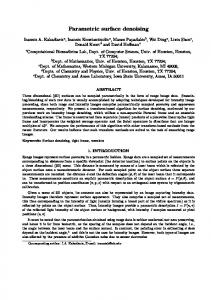
Chapter 1 Introduction Recent innovations and developments in 3D acquisition technology, such as 3D laser scanners, magnetic resonance imaging, ultrasound, optical coherence tomography and LiDAR scanning allow fast, robust and highly accurate digitization of complex 3D objects. The analysis and processing of these geometric data are vital in various scientific disciplines and industries, such as neuroscience, mechanical engineering, animation, etc. Discrete differential geometry, a relatively new field in mathematics and computer science that concerns between acquisition and production of a geometrical data. Discrete differential geometry is a rapidly growing research field, equipped with concepts of classical and modern differential geometry of smooth manifolds, mathematical models and algorithms for analyzing and manipulating geometric data. Geometry processing is basically a combination of several mathematical algorithms, which are applied to geometrical models in various real life applications, for example, Figure 1.1 shows a general pipeline for geometry processing.

Figure 1.1: A general pipeline for geometry processing. The thesis is divided in two parts. The first part consists of Chapter 2−5. In this part, we introduce a shape analysis operator (Chapter 2), its application to mesh denoising (Chapter 3) and point set denoising (Chapter 4). This thesis also discusses about the robust statistics framework and introduces a robust and high fidelity mesh denoising using a robust estimator (Chapter 5). In the second part, we apply geometry processing algorithms including the proposed algorithm in the first part of thesis, for the retinal shape analysis. An general introduction about a human eye, the retinal shape and common neurological disorders are given in Chapter 6. Chapter 7 comprises of an algorithm to perform a parametric modeling of the fovea, which is an important region in 1

2

Chapter 1 Introduction

the retina. The optical nerve head morphometry is performed in Chapter 8 using the proposed geometry processing algorithms. Here, we give an introduction about surface denoising, general problems in surface denoising and an overview of state-of-the-methods related to these topics. Surface Denoising: Surface denoising is a central preprocessing tool in discrete geometry processing with many applications in computer graphics such as CAD, reverse engineering, virtual reality and medical imaging. During a surface measurement, noise is inevitable due to various internal and external factors and this degrades surface data quality and its usability. The main goal of a surface denoising algorithm is to remove spurious noise and compute a high quality noise-free surface while preserving sharp features. In general, noise and sharp features both have high frequency components, so decoupling the sharp features from noise is still a challenging problem in surface denoising algorithms. Traditionally, noise is removed by using a low pass filtering approach, but this operation leads to feature blurring as shown in Figure 1.2. Noise behaviour depends highly on resolution and uniformity of the corresponding mesh. As it can be seen from Figure 1.2(e), feature preservation is a challenging task with non-uniform meshes and also the removal of low frequency noise is not so straight forward (Figure 1.2 (e), top edge of the cylindrical region). Figure 1.2 (f) shows the result obtained by our method [114], which produces a noise-free mesh with sharp features.

(a) Original

(b) Noisy

(c) Blurring

(d) Shrinkage

(e) Non-uniform (f) Ours [114] mesh effect

Figure 1.2: General problems in mesh denoising. Retinal Shape Analysis: In this part of thesis, we introduce couple of geometric processing algorithms for quantification of the retinal shape. As part of the central nervous system, the retina comprises a similar cellular composition as the brain, and many neurological disorders thus affect the retina. Many neuroinflammatory conditions are known to cause modifications to two important regions of the retina: the fovea and the optical nerve head (ONH) and an accurate and robust shape modeling of these regions can diagnose several neurological disorders by detecting the shape changes. A detailed discussion about this part is mentioned in Chapter 6, 7 and 8.

1.1

Main Contributions

The main contributions of this thesis have been divided into two parts: mesh and point set denoising in a proposed normal voting tensor framework and the retinal shape analysis, which includes a parametric modeling of the foveal region and a quantification of the optical nerve head region.

1.1 Main Contributions

3

Surface Denoising and Feature Analysis • We follow the variation of surface normals, which is termed as the normal voting tensor and derive a relation between the shape operator and the normal voting tensor. • We extend the concept of the directional and the mean curvatures on the dual representation of a triangulated surface using the proposed element-based normal voting tensor (ENVT). • We propose an ENVT-based mesh denoising algorithm. A binary optimization technique is applied on the spectral components of the ENVT that helps the algorithm to retain sharp features in the concerned geometry and improves the convergence rate of the algorithm. • We give a stochastic analysis of the effect of noise on a triangulated mesh based on the minimum edge length of elements in the geometry. It gives an upper bound to the noise standard deviation to have minimum probability for flipped element normals. • We investigate the robust statistics framework for face normal bilateral filtering and propose a robust and high fidelity two-stage mesh denoising method using Tukey’s bi-weight function as a robust estimator to stop the diffusion at sharp features and to produce smooth umbilical regions. • We introduce a vertex update scheme, which uses a differential coordinate-based Laplace operator along with an edge-face normal orthogonality constraint to produce a high-quality mesh without face normal flips and this operator also makes the algorithm more robust against high-intensity noise. • We extend the concept of the ENVT-based mesh denoising for a point set denoising algorithm, where noisy vertex normals are filtered using the vertex-based NVT and the binary optimization. • For vertex update stage in point set denoising, we add different constraints to the quadratic error metric based on features (edges and corners) or non-feature (planar) points. Retinal Shape Analysis • We introduce a parametric modeling of the foveal shape using Cubic Beziér and derive several 3D shape parameters to quantify the foveal shape with high accuracy. • A 3D shape analysis algorithm is introduced to measure the shape variation in the ONH in different neurological disorders. The proposed method uses manifold surfaces of two different layers of the retina to derive several 3D shape parameters. Publications

Parts of this thesis appear in the following papers:

• ”Mesh Denoising based on Normal Voting Tensor and Binary Optimization”, IEEE Transactions on Visualization and Computer Graphics 2017 [114]. DOI: https://doi.org/10.1109/TVCG.2017.2740384. • ”Cube: Parametric Modeling of 3D Foveal Shape using Cubic Bézier”, Biomedical Optic Express 2017 [112]. DOI: https://doi.org/10.1364/BOE.8.004181.

4

Chapter 1 Introduction • ”Constraint-based Point Set Denoising using Normal Voting Tensor and Restricted Quadratic Error Metrics”, Computer and Graphics 2018 (Shape Modeling International 2018) [116]. DOI = https://doi.org/10.1016/j.cag.2018.05.014 . • ”Robust and High Fidelity Mesh Denoising”, IEEE Transactions on Visualization and Computer Graphics 2018 [115]. DOI: https://doi.org/10.1109/TVCG.2018.2828818. • ”Optic Nerve Head 3D Shape Analysis”, submitted to IEEE Transactions on Medical Imaging 2018 [113].

1.2

Related Work in Surface Denoising

In last two decades, a wide variety of smoothing algorithms have been introduced to remove undesired noise while preserving sharp features in a geometry. The most common technique for noise reduction is mainly based on the Laplacian on surfaces. We can characterize them as isotropic, anisotropic and two stage smoothing methods. For a comprehensive review on mesh denoising, we refer to couple of survey papers [14–16]. We mention a major part of related works in this section. Isotropic smoothing methods are the earliest smoothing algorithms. These algorithms have low complexity but suffer from severe shrinkage and further feature blurring [32]. Desbrun et al. [21] introduced an implicit smoothing algorithm that produces stable results for irregular meshes and avoids the shrinkage by volume preservation. Later, the concept of the differential coordinates is introduced by Alexa [4] as a local shape descriptor of a geometry. Differential coordinates preserves the fine details on a triangular mesh, which leads to their further applications in mesh processing, for example, Lipman et al. [63] used the same concept for mesh editing. Mesh quantization [93] and Shape approximation [92] are also done by using the concept of differential coordinates. Sorkine et al. [91] introduced a general differential coordinate-based framework for mesh processing. In continuation, vertex-based Laplacian mesh optimization algorithm was introduced by Nealen et al. for shape optimization and mesh smoothing [72]. Later, Su et. al. exploited the differential coordinates concept for mesh denoising by computing the mean of the differential coordinates at each vertex [94]. This method produces less shrinkage but is unable to preserve shallow features. In general, isotropic smoothing methods are prone to shrink volumes and blur features but effective in noise removal. Anisotropic diffusion is a PDE based de-noising algorithm introduced by Perona and Malik [82]. The same concept was extended for surface denoising using a diffusion tensor [7, 20]. Similarly, the anisotropic diffusion of surface normals was introduced for surface smoothing [99]. Later, the prescribed mean curvature based surface evolution algorithm was introduced by Klaus et al. [45] that avoids the volume shrinkage and preserves features effectively during the denoising process. The bilateral filtering was initially proposed by Tomasi et al. [103] for image smoothing. The relation between anisotropic diffusion [45] and the bilateral filtering is explained by Barash [9]. In continuation, Black et al. [13] and Durand et al. [24] expressed anisotropic diffusion and the bilateral filtering in a robust statistics framework [42]. The concept of bilateral smoothing was extended for mesh denoising by Fleishmann et al. [34] and later, Jones et al. [51] explained the same concept in a robust statistics framework. A consistent subneighborhood-based bilateral filtering is introduced by Fan et al. [29]. Solomon et al. proposed a general framework for bilateral and mean shift filtering in any arbitrary domain [90]. These algorithms are simple and effective against noise and feature blurring. In general, anisotropic denoising methods are more robust against volume

1.2 Related Work in Surface Denoising

5

shrinkage and are better in terms of feature preservation but the algorithm complexity is higher compared to isotropic algorithms. The two step denoising methods are simple and quite robust against noise. These algorithms consist of two steps: the face normal smoothing and the vertex position update. Face normals are treated as signals on the dual graph of a mesh with values in the unit sphere. The Laplacian smoothing of face normals on a sphere is introduced by Taubin [101] and displacement of the concerned face normal is computed along a geodesic on the unit sphere. The face normal smoothing is done by rotating a face normal on the unit sphere according to the weighted average of neighbor face normals. The bilateral surface normal filtering with the least squares error vertex position update was introduced by Lee et al. [58]. Later, different linear and non-linear weighting functions have been introduced by different algorithms for the face normal smoothing. For example, Yogou et al. [117] computed the mean and the median filtering of face normals to remove noise effect. Later, a modified Gaussian weighting function was applied to the face normal smoothing in an adaptive manner to reduce features blurring [78]. In continuation, the alpha trimming method introduced a non-linear weighting factor which approximates both, the mean and the median filtering [117]. Bilateral normal is one of the most effective and simple algorithms among the two step methods [121], where the weighting function is computed based on the normal differences (similarity measurement) and spatial distances between neighboring faces. Recently, a total variational method has been introduced for the face normal filtering [119]. After the preprocessing of face normals, the vertex position update is done by using the orthogonality between the corresponding edge vector and the face normal [95]. Wang et al. [106] introduced a learning-based mesh denoising algorithm, where the bilateral filtered normal descriptor is used to model the local geometry features. The two step denoising methods are simple in implementation and produce effective results. However, on noisy surfaces, it is difficult to compute the similarity function because of the ambiguity between noise and sharp features, and that leads to unsatisfactory results. In recent mesh denoising methods, compressed sensing techniques are involved to preserve sharp features precisely and remove noise effectively [111]. For example, L0 mesh denoising method assumed that features are sparse on a general surfaces and introduced an area based differential operator. This method utilizes L0 optimization to maximize flat regions on a noisy surfaces to remove noise [43]. The L0 method is effective against high noise but produces piecewise flat areas on smooth surfaces. Later, the weighted L1 -analysis compressed sensing optimization is applied to recover sharp features from the residual data after global Laplacian smoothing [107]. Recently, the ROF-based (Rudin, Osher and Fatemi) algorithm has been introduced in [110]. This method applies L1 optimization on both data fidelity and regularization to remove noise without volume shrinkage. In continuation, Lu et al. utilized the L1 -median normal filtering along with vertex preprocessing to produce a noise-free surface [66]. Recently, Yadav et al. [114] proposed a binary optimization-based mesh denoising algorithm, where noise was removed by assigning a binary values to a face normal-based covariance matrix. Centin et al. [16] proposed a normal-diffusion-based mesh denoising algorithm, which removes noise components without tempering the metric quality of a surface. In general, the compressed sensing based denoising algorithms are robust against high intensity noise and recover not only sharp features but also shallow features, but at the same time these algorithms produce false features (piecewise flat areas) on smooth geometries. A multistage denoising framework was introduced by Bian et al. [12], where feature identification is done by the eigenalysis of the NVT (normal voting tensor) [55] [70] and then geometry is divided into different clusters based on features and smoothing is applied on different clusters independently. Later, the guided mesh normals are computed based on consistence normal orientations and the bilateral filtering is applied [120]. Recently, Wei et al. [108] exploited both vertex and face normal information for feature classification and surface smoothing. In continuation, fea-

6

Chapter 1 Introduction

tures detection is done on the noisy surface using quadratic optimization and remove noise using L1 optimization while preserving features [67]. Multistage denoising algorithms produce effective results against different levels of noise but have higher algorithm complexity because of the different stages. Similar to mesh denoising, point sets denoising is also studied by several researchers in last two decades [10]. The moving least squares was introduced by Alexa et al. [5] to up-sample a point set in local tangent spaces. Later, a parametrization free, local optimal projector is introduced to remove noise and outliers from point sets using the L1 -median [62]. LOP concept was modified by Huang et al. by adding the weighting term, which makes the algorithm robust against non-homogeneous point density [48]. Algebraic Point Set Surfaces (APSS) algorithm used local moving least squares to reconstruct a smooth surface from a point set [40]. In continuation, RIMLS (robust implicit ¨ moving least squares) was introduced by Oztireli et al. and it preserves sharp features by applying bilateral normal filtering before projection [80]. Lange and Polthier [57] introduced the anisotropic smoothing of point sets using the shape operator and principal curvatures. In terms of feature preservation, L0 point set denoising is introduced by Sun et al. [97] and this algorithm recovers sharp features by computing piecewise flat areas on a point set surface. In continuation, Mattei et al. [68] introduced MRPCA (moving robust PCA) to remove outliers effectively and retain sharp features. Recently, a guided point set denoising algorithm is introduced. This method exploited L1 -median skeleton to extract the feature points and then computed guidance normal by using consistent normals [122].

Chapter 2 Element-based Normal Voting Tensor (ENVT) On a polygonal mesh surface, estimation of curvature informations including, principal curvatures is quite important for various geometry processing algorithms, for example, shape analysis, mesh segmentation and surface smoothing. In the past, several shape analysis operators have been introduced for feature detection and basic geometry processing operations, for example, the curvature tensor, which was introduced by Taubin [100] and it computes the variation of tangent vectors along a curve on a triangulated surface. The spectral analysis of the curvature tensor approximates the principal curvatures of polygonal surfaces. We follow similar concept and introduce the variation of surface normals termed as the normal voting tensor, and derive a relation between the shape operator and the normal voting tensor. We extend the concept of the directional and the mean curvatures on the dual representation of a triangulated surface. A normal voting tensor is defined on each triangle of a geometry and termed as the element-based normal voting tensor (ENVT). Later, a deformation tensor consisting of the anisotropy of a surface is extracted from the ENVT, and the mean curvature vector is defined based on this ENVT deformation tensor. We also show a similarity of the ENVT with the principal directions and the principal curvatures. In the end of this chapter, we experimented the capability of the ENVT in terms of feature preservation.

2.1

The Curvature Tensor

The curvature notion has a central importance in classical differential geometry and has several concepts and definitions. Here, we explain the concept of directional (normal) curvature using the classical Meusnier’s theorem. Theorem 1. (Meusnier’s theorem) Let M ⊂ R3 be a orientable regular surface with unit normal field N : M → R3 and second fundamental form II : Tp M × Tp M → R, where Tp M is the tangent plane at a point p ∈ M spanned by principal curvature directions T1 and T2 as the orthonormal basis. Let c : (−, ) → M be a curve parametrized by arc-length with c(0) = p, then the directional (normal) curvature of c can be expressed as: κp = II(c(0), ˙ c(0)). ˙ (2.1) Let us consider an arbitrary vector Tθ ∈ Tp M, which can be expressed in terms of the orthonormal basis T1 and T2 : Tθ = {cosθT1 + sinθT2 }, θ ∈ R, (2.2) Let us assume that the curve c is aligned with the tangent vector Tθ , then Tθ = c(0). ˙ By differential geometry, the shape operator has a diagonal form and because of the orthogonality of the curvature 7

8

Chapter 2 Element-based Normal Voting Tensor (ENVT)

line parametrization, the second fundamental form computes the directional curvature w.r.t. Tθ ∈ Tp M, and this directional curvature can also be expressed in a quadratic form:

κp (Tθ ) = II(Tθ , Tθ ) = cosθ sinθ

κ 1

0 κ2

0

!

!

cosθ . sinθ

(2.3)

Substituting the value of Tθ from Equation (2.2) into second fundamental form gives us the Euler formula for the directional curvature: κp (Tθ ) = II(Tθ , Tθ ) = κ1 cos2 θ + κ2 sin2 θ.

(2.4)

Using the directional curvature from Equation (2.4) and an arbitrary tangent vector Tθ , Taubin [100] introduced the curvature tensor at point p on a surface M, which is defined as: Mp =

1 2π

Z

+π

−π

κp (Tθ )Tθ Ttθ dθ,

(2.5)

where Tθ is a column vector. The curvature tensor Mp is a covariance matrix of a set of tangent vectors, where each tangent vector is weighted by the corresponding directional curvature. The curvature tensor is rewritten in following form using Equations (2.2) and (2.4): 1 Mp = 2π

Z

+π

−π

(κ1 cos2 θ + κ2 sin2 θ)(cosθT1 + sinθT2 )(cosθT1 + sinθT2 )t dθ.

(2.6)

The term Mp is a 3 × 3 matrix and we can decompose this tensor in terms of the orthonormal basis T1 and T2 of the tangent plane Tp M:

Mp = T1 T2

σ 2

0

0 σ3

!

!

Tt1 , Tt2

(2.7)

where T1 and T2 are the column vectors, thus, (T1 , T2 ) will be a 3 × 2 matrix. The non-diagonal components of the eigenvalues matrix (2 × 2, the central matrix) are zero. Using Equation (2.6), the eigenvalues (σ2 and σ3 ) of the tensor Mp are computed as: 1 3 σ2 = Tt1 Mp T1 = κ1 + κ2 , 8 8

1 3 σ3 = Tt2 Mp T2 = κ1 + κ2 . 8 8

(2.8)

The above equation shows a relationship between the principal curvatures and the eigenvalues of the curvature tensor. The mean curvature is defined as the arithmetic mean of the principal curvatures. κ1 + κ2 κ1 = 3σ2 − σ3 , κ2 = 3σ3 − σ2 , H = = σ2 + σ3 . (2.9) 2 The eigenvectors of Mp are aligned with the principal directions but its eigenvalues are not approximating the principal curvatures, for example, on a cylinder both of these eigenvalues are non-zero but the minimum principal curvature is zero. The eigenvalues σ2 and σ3 can have negative values also and approximate the mean curvature effectively. Let us consider, for a particular value of θ in the radial direction, point q is lying on the same surface M in the neighbourhood of p. Let us consider an arc-length parametrized smooth curve c between p and q such that the tangent direction Tθ = c(0) ˙ and the directional curvature κp (Tθ ) = c¨(0)np , where np ∈ N is the surface normal at point p then, by using Taylor series expansion the directional curvature from p to q can be approximated as: κp (Tθ ) =

2hnp , (q − p)i . |q − p|

(2.10)

9

2.2 Normal Voting Tensor (NVT)

Vertex-based Directional and Mean Curvatures on a Triangulated Surface In the discrete setting, let us consider a triangulated surface M = (V, F), which is a combination of a set of vertices and a set of elements. For a vertex vi ∈ V, the directional curvature w.r.t. vj ∈ Ni , and mean curvature can be defined as: κij =

2hnvi , (vj − vi )i , |vj − vi |

H=P

1

j∈Ni

X

Wij

Wij κij ,

(2.11)

j∈Ωi

where Ni is the set of neighbour vertices of vi . The term H is mean curvature and Wij is a weighting factor associated with each neighbor vertex. In general, this weighting factor is chosen on the basis of an area of elements connected with the vertex vi . The corresponding tangent plane is computed using the vertex normal nvi .

2.2

Normal Voting Tensor (NVT)

In general, covariance matrices compute a variation of an entity in a well defined domain, for example, principal component analysis (PCA), where the covariance matrix of an edge vector on a triangular surface computes the variation of vertices in R3 space. The curvature tensor Mp is a weighted covariance matrix, which computes the variation of tangent vectors around a point. In general, surface normals carries anisotropy of a surface hence a covariance matrix of surface normals in a well defined neighborhood computes anisotropic nature of a surface in that region. To analyze anisotropy of an orientable surface M ⊂ R3 , which has well defined normal field N : M → R3 , for any Ω ⊂ M, we define a bilinear form CΩ : Ω × Ω → R. In most general term, we have a map: Ω 7→ CΩ , where Ω is a geodesic disk of radius r. Now, we define the term CΩ in terms of the tensor product (outer product) of surface normals: 1 CΩ = |Ω|

Z

n ⊗ ndΩ,

(2.12)

Ω

where n ∈ N is a column vector and is an order-1 tensor. The symbol ⊗ represents the outer product, which can be written as n ⊗ n = nnt . The term CΩ is known as the normal voting tensor. The above equation shows a special case of the Kronecker product of matrices and possesses the following properties: 1. The inner product of normal vectors can be computed using the trace of the outer product. 1 |Ω|

Z

hn, nt idΩ = Trace(CΩ ).

(2.13)

Ω

2. If the surface normal n is a non-zero vector then CΩ has matrix rank 1 because for any vector x ∈ R3 : Z 1 CΩ x = n(nt x)dΩ, (2.14) |Ω| Ω where (nt x) is a scalar quantity. 3. As the surface normal n is an order-1 tensor so the term CΩ will be an order-2 tensor. As it is mentioned in Equation (2.12), CΩ is a covariance matrix of surface normals so the normal voting tensor computes the variation of surface normals in Ω geodesic disk. To understand this variation, we follow a theorem by Rodriguez from classical differential geometry.

10


Theorem 2. (Rodriguez’s theorem) Let M ⊂ R3 be a orientable regular surface and n belong to a unit normal field N : M → R3 . Let c : I → M be a curve parametrized by arc-length, then c is a curvature line on M if and only if there exists a function λ : I → R with: d n(c(t)) = λ(t) · c(t), ˙ dt

t ∈ I,

(2.15)

where −λ(t) is the corresponding principal curvature. From Rodriguez’s theorem, it is clear that the variation of normals depends on mainly two factors: tangent direction c(t) ˙ and corresponding principal curvature. A similar conclusion, we get from Weingarten map Wp : Tp M → Tp M as well: Wp (Ti ) = κi · Ti ,

i = 1, 2.

(2.16)

From Equations (2.15) and (2.16), it is clear that the variation of surface normals is well approximated in the principal directions using the principal curvatures. However, it is not so clear in arbitrary directions. For θ ∈ [−π, π), let cθ : (−, ) → Ω be a unit speed geodesic along which we study the change of the normal vector. Using Taylor expansion: n(cθ (t)) = n(cθ (0)) + tn(cθ (0))0 + O(t2 ),

(2.17)

where the term n(cθ (0))0 is similar to Equation (2.15) and represents the corresponding tangent vector, which is defined in the local neighborhood of point p: ˜ θ = κ1 cosθT1 + κ2 sinθT2 . T

(2.18)

In the above equation, we added the principal curvatures κ1 , κ2 as weighting factors in the principal ˜ θ is spanned by the directions T1 , T2 to create an anisotropic radial sampling. The tangent vector T principal curvature directions and is closer to the maximum principal direction than the minimum principal direction. ˜ θ (Equation (2.18)), which is the The term n(cθ (0))0 (Equation (2.17)) can be replaced with T combination of the principal directions and curvatures. The radius term r defines the neighborhood area and as r → 0, the surface normal n(cθ (0)) = n0 . For a small disk radius the higher order component will be close to zero O(t2 ) ≈ 0 and the surface normal can be written as a linear ˜ θ. combination of n0 and its corresponding tangent plane T ˜ θ. n(cθ (t)) = n0 + tT

(2.19)

In other words, when we move in arbitrary direction Tθ as mentioned in Equation (2.2), the ˜ θ in first order approximation. From Equations (2.12) and (2.19), we surface normal changes by T express the NVT in the following integral equation in a polar coordinate form around a point p: 1 CΩ = 2 πr

Z

π

r

Z

−π

˜ θ ) ⊗ (n0 + tT ˜ θ )tdtdθ, (n0 + tT

(2.20)

0

where geodesic disk area |Ω| = πr2 . Using Equations (2.18) and (2.20): CΩ = n0 ⊗ n0 +

r2 4π

Z

π

−π

(κ21 cos2 θT1 ⊗ T1 + κ22 sin2 θT2 ⊗ T2 )dθ.

(2.21)

So the ENVT can be decomposed into two different covariance matrices: CΩ = C0 +

r2 Cκ , 2

(2.22)

2.3 Element-based Normal Voting Tensor (ENVT) on a Triangulated Surface

11

where C0 is the covariance matrix regarding n0 (when r → 0) and has only one dominant eigenvalue in the surface normal direction. The second term Cκ consists of the variation of surface normals excluding n0 within disk Ω. The NVT CΩ is a symmetric positive semi-definite matrix and can be written in terms of orthonormal basis: 



CΩ = n0 T1 T2



n0 λ1 0 0     0 λ2 0  T1 , T2 0 0 λ3

(2.23)

and the most dominant eigenvalue along the surface normal is computed using the following equation: λ1 = n0t CΩ n0 = 1. (2.24) In this case, Cκ will be a zero covariance matrix because it has zero eigenvalue along the surface normal direction and non-zero eigenvalues along the principal directions, which are perpendicular to n0 . The other two eigenvalues along the principal directions can be computed as: λ2 = Tt1 CΩ T1 =

r2 t r2 1 T1 Cκ T1 = 2 2 2π

Z

λ3 = Tt2 CΩ T2 =

r2 1 r2 t T2 Cκ T2 = 2 2 2π

Z

π

−π π

−π

κ21 cos2 θdθ =

r2 κ21 , 4

(2.25)

κ22 sin2 θdθ =

r2 κ22 , 4

(2.26)

From the above equations, it is clear that second and third eigenvalues of the NVT approximate squares of the principal curvatures κ1 and κ2 . The eigenvalues (σ2 , σ3 ) of the curvature tensor are a linear combination of the principle curvatures (κ1 , κ2 ). Considering the same example of Cylinder, unlike σ3 , which is non-zero, the least dominant eigenvalue λ3 of the NVT will be zero. Therefore, the NVT approximates the shape operator better compared to the curvature tensor.

2.3

Element-based Normal Voting Tensor (ENVT) on a Triangulated Surface

The concept of normal voting was introduced by Medioni [70] and was used in various computer vision applications. The basic idea of normal voting tensor is to select the neighborhood of a vertex and these neighborhood vertices vote to estimate feature points on a surface. As face normals are a first order information on a surface and give better description about sharp features than vertex normals because the angles between face normals are bigger compared to the angles between vertex normals in those regions. We extended the normal voting concept and define an element-based normal voting tensor on every element of a properly oriented triangulated mesh. Similar to Section 2.2, the element-based normal voting tensor is the weighted average of the outer product of the neighbor element normals. On the geometrical neighborhood Ωi of face fi (Figure 2.1), the ENVT is defined as: CΩi = P

X 1 wij Aj nj ⊗ nj , j∈Ωi wij Aj j∈Ω

(2.27)

i

where Aj is the area of fj and wij is a Gaussian-based weighting function. Weighting by corresponding element area makes the proposed tensor more robust against irregular sampling. The element

12


based normal voting tensor is a symmetric and positive semi definite matrix so, we can represent CΩi using a rotational and a scaling matrix: 



CΩi = RΛRt = e1 e2 e3



e1 λ1 0 0     0 λ2 0  e2  , e3 0 0 λ3

(2.28)

where R and Λ are the rotational and the scalar matrix respectively. The terms ei and λi are spectral components of the ENVT.

Ωi ci Vi

r

cj Vj

(a) Triangulate mesh

(b) Dual Mesh

(c) Both

Figure 2.1: A visual representation of primal and dual mesh. (a) Original mesh M, where the vertex vj ∈ Ni belongs to the 1-ring neighborhood of vertex vi . (b) Dual polyhedral mesh Md , which is computed from triangulated mesh M using Equation (2.31). The geometrical neighborhood is represented by Ωi , which is a disk of radius r on the dual mesh. (c) Both triangulated and corresponding dual mesh. As it can be seen from Equation (2.28), the eigenvectors e2 and e3 are the basis of a tangent space and align with the principal directions (T1 = e2 , T2 = e3 ). The eigenvector e1 aligns with the surface normal at that point as shown in Figure 2.2.

e3 e1

(a) Eigenvalues of C and B

e2

(b) Magnified view

Figure 2.2: The eigenvectors visualization on a Cube model. (a) The eigenvectors are painted on Cube, e1 in green, e2 in blue and e3 in red for both the ENVT and the deformation tensor. (b) The least dominant eigenvector e3 is aligned with the edge direction, which is the minimum principal direction.

13

2.4 Feature Analysis based on the ENVT

2.4

Feature Analysis based on the ENVT

The ENVT primarily consist of the anisotropy of a triangulated surface and can be written in terms of its spectral components: CΩi = (λ1 − λ2 )e1 ⊗ e1 + (λ2 − λ3 )(e1 ⊗ e1 + e2 ⊗ e2 ) + λ3 (e1 ⊗ e1 + e2 ⊗ e2 + e3 ⊗ e3 ), (2.29) where the eigenvalues are sorted in decreasing order: (λ1 ≥ λ2 ≥ λ3 ≥ 0). As shown in Figure 2.3, each term of Equation (2.29) can be defined as the following tensors: 1. The term (λ1 − λ2 )e1 ⊗ e1 is defined as the stick tensor because this tensor has a stick like shape in the surface normal direction. 2. The term (λ2 −λ3 )(e1 ⊗e1 +e2 ⊗e2 ) is defined as the plate tensor because the two eigenvectors are spanning a plate like shape and the least dominant direction will be normal to this plate like shape. 3. The term λ3 (e1 ⊗ e1 + e2 ⊗ e2 + e3 ⊗ e3 ) is defined as the ball tensor because this tensor is spanned by all three eigenvectors. Based on these tensors, we can define the saliency of features on a surface. The stick tensor represents the surface saliency (SMap) where the surface normal is in the direction of the most dominant eigenvector and (λ1 − λ2 ) shows the strength in that direction. Similarly, the plate tensor is the socalled curve map (CMap) and has two dominant eigenvector. The ball tensor basically represents the intersection of more than two planes and has no well defined direction either for surface normal or for surface tangent and is so-called junction map (JMap) [70]. On a noise free triangulated mesh, a planar area has only one dominant eigenvalue in surface normal direction (SMap) and the least dominant eigenvectors represent an orthonormal basis for the tangent plane. Two dominant eigenvalues indicate edge features (CMap), where the weakest eigenvector will be along the edge direction and dominant eigenvalues are in the direction of the surface normal and across the edge respectively. Therefore, the tangent space will be spanned by significant and insignificant directions. At a corner all three eigenvalues are dominant (JMap) and it is not trivial to define a tangent plane. Let us consider the Cube model, and compute the ENVT using Equation (2.28). The eigenvalues vector is sorted and√normalized, then for orthogonal features,√we can write: {λ1 = 1, λ2 = λ3 = 0} (face), {λ1 = λ2 = 22 , λ3 = 0} (edge) and {λ1 = λ2 = λ3 = 33 } (corner). Let us define a new eigenvalues vector λp = {1, λλ21 , λλ31 } and categorize the following features points: 1. Significant value of

λ3 λ1

indicates a corner point.

2. Significant value of

λ2 λ1

indicates a edge.

3. On planar areas,

λ2 λ1

and

λ3 λ1 ,

both are insignificant.

Using the above classification, we can define the feature strength value: sf = λ2 + λ3 .

(2.30)

Figure 2.4(c) shows a visual representation of the feature strength on a smooth Fandisk model. As it can be seen, the ENVT identifies sharp features effectively.

14


{λ1, e1}

{λ2, e2}

{λ1, e1}

{λ2, e2}

{λ1, e1}

{λ3, e3}

(a) JMap

(b) CMap

(c) SMap

(d) Together

Figure 2.3: A visual representation of different kinds of tensors mentioned in Equation (2.29).

2.5

Curvature Approximation in the ENVT Framework

In the discrete setting, the curvature tensor is well defined for vertices on a triangulated mesh and it approximates the directional and the mean curvatures with high fidelity. Here, we exploit a similar framework to define the directional and the mean curvatures on elements (faces) of a surface. Firstly, we compute a barycentric dual mesh Md of the original triangulated surface M. The dual mesh Md will be a polyhedral surface and consists of vertices and polygon elements. For the dual mesh Md , the set of vertices and elements are represented as Vd and Fd respectively. Each vertex of the dual mesh has a fixed connectivity of 3 and can be computed as: ci =

1 X vj , 3 v ∈f j

where

fi ∈ F,

vj ∈ V.

(2.31)

i

Note that elements in the dual mesh will be n-sided polygon and number of sides in polygons depends on vertices connectivity in the original triangulated surface as shown in Figure 2.1. Each vertex ci of the dual mesh has a well defined vertex normal ni , which is basically the face normal of the element fi ∈ F in the original triangulated surface. Patanè et al. [81] discussed a homeomorphism between 2-manifold tringulated mesh and its dual representation and the several combinatorial properties of a dual mesh, which include 1-neighborhood analysis, triangle mesh reconstruction, primal-dual correspondence and dual Laplacian smoothing. The dual transformation is also genus invariant for polygonal mesh. Similar to Equation (2.11), the directional and the mean curvatures on the dual mesh Md is defined as: κdij =

2hni , (cj − ci )i , |cj − ci |

Hd = P

1 j∈Ωi Wij

X

Wij κdij ,

(2.32)

j∈Ωi

where Wij = Aj is the area of fi ∈ F. To compute the direction curvature κdij , we need to compute the tangent plane Tij , which is basically the triangle plane of fi ∈ F and is computed using the face normal ni . The area weighting will improve the accuracy of curvatures computation as big area elements have trustworthy normals. The ENVT C is a positive semi-definite symmetric matrix and can be expressed in a form of the deformation tensor B: C = BBt s.t. det(B) > 0. (2.33) From Equations (2.27) and (2.33), the deformation tensor is defined in terms of the rotation and the scaling matrix: 1 1 1 C = RΛ 2 Λ 2 Rt = BBt , and B = RΛ 2 . (2.34)

15

2.5 Curvature Approximation in the ENVT Framework

Using the above representation of the ENVT, for a given vector u, we can express the ENVT in the following quadratic form : ut Cu = ut BBt u = (Bt u)t (Bt u) = kBt uk2 .

(2.35)

By using the above representation of the ENVT, similar to Tsuchie et al. [104], a distance between central vertex ci and neighbor vertex cj on the dual mesh is defined as: dij =

q

(cj − ci )C(cj − ci )t = kBt (cj − ci )k,

(2.36)

where the parameter dij possesses the following properties: 1. In general, dij 6= dji . 2. If ci and cj have the same tangent plane then dij = 0, because dij compute a distance in the surface normal direction. 3. If the ENVT is an identity matrix then, dij represent an Euclidean distance in R3 . The deformation tensor B carries anisotropy nature of a surface and can be used to approximate the direction curvature along with dij : √ t X 2B (cj − ci ) d ¯d = P 1 κ ¯ ij = Wij κdij , (2.37) , H W |cj − ci | ij j∈Ω j∈Ωi i

¯ d ) curvatures using the anisoThe above equations present the directional (¯ κdij ) and the mean (H tropic deformation tensor and vertex positions of the dual mesh.

(a) Cotangent MC

(b) Hd (Equation (2.32))

(c) sf (Equation (2.30))

¯ d (Equation (2.37)) (d) H

Figure 2.4: A visual representation of different kinds of feature analysis operator. (a) traditional mean curvature computed using the shape operator. (b) mean curvature computed using Equation (2.32) on the dual mesh of the Fandisk model. (c) Edges and corners are detected using the eigenanalysis of the ENVT. (d) feature detection using the ENVT deformation tensor as a mean curvature operator. The deformation tensor B and the ENVT both have the same eigenbasis. The eigenvalues of the deformation tensor are square roots of the eigenvalues of the ENVT, so it can also be written in its spectral components: B=

3 p X

λi ei eti .

i=1

(2.38)

√ √ Here, λ2 and λ3 approximate the principal curvature, and the corresponding eigenvectors are the principal directions. In Figure 2.2, the least dominant and the most dominant eigendirection e3

16


are colored in red and green respectively. The eigenvalue e2 is painted in blue color. Figure 2.2 (b) shows that the least dominant direction (e3 ) is along the edge and the eigenvalue λ3 corresponding to this direction is equal to zero. The most dominant eigendirection (e1√ ) approximates the surface normal and across the edge-direction, there will non zero eigenvalue λ2 . The tangent space is spanned by the two least dominant directions. Here, we can say that the lower sub-matrix of the deformation tensor approximates the shape operator.

2.6

Summary

In this chapter, a shape analysis operator, the ENVT is introduced. The spectral analysis of the ENVT revealed that it can be decomposed into several feature based tensors, for example, stick, plate and ball tensors. To identify feature points on a triangulated surface, a feature strength parameter sf is introduced and Figure 2.4 (c) shows that sf detects sharp features on a geometry effectively. Later, the concept of dual mesh is exploited to derive the mean curvature operator and the directional curvature based on face normals and barycentric points of the corresponding faces. With help of the deformation tensor, which is decomposed from the ENVT, a metric and mean curvature vector is again computed. In the end, similar to the curvature tensor by Taubin [100], correlation between the shape operator and the ENVT is presented and it is shown that two least dominant eigenvalues of the ENVT approximate the squared principal curvatures and corresponding eigenvectors are the principal directions.

Chapter 3 ENVT-based Mesh Denoising Algorithm In general, noise and sharp features both are high frequency components and decoupling them during a denoising operation, is a challenging task. Several traditional average-based denoising methods have been published to remove noise effectively. However, they are not able to preserve sharp features properly because of the ambiguity between noise and sharp features. Unlike other traditional averaging approaches, our method uses the element-based normal voting tensor to compute smooth surfaces. By introducing a binary optimization on the tensor together with a local binary neighborhood concept, the algorithm better retains sharp features and produces smoother umbilical regions than previous approaches. On top of that, a stochastic analysis on the different kinds of noise is provided based on the average edge length. The quantitative results demonstrate that the performance of our method is better compared to state-of-the-art smoothing approaches. This chapter is based on a published mesh denoising method [114]. Additionally, we added the detailed denoising explanation in 1D using a noisy polygon including a graphical description of the ENVT multiplication to the noisy face normal. The definitions of different kinds of neighborhood are included. We shortened the properties and explanation of the ENVT as it is well explained in Chapter 2. This algorithm follows a two stage denoising process. In the first stage, noisy face normals are processed to remove undesired noisy component and in the second stage, vertex positions are updated according to processed face normals. The main contributions of this chapter are: • A tensor-based mesh denoising algorithm is introduced to remove the undesired noise from noisy surfaces with a stable and fast convergence property. • A binary optimization technique is applied on the eigenvalues of the proposed element-based normal voting tensor (ENVT) that helps us to retain sharp features in the concerned geometry and improves the convergence rate of the algorithm. • We give a stochastic analysis of the effect of noise on a triangular mesh based on the minimum edge length of elements in that geometry. It gives an upper bound to noise standard deviation to have minimum probability for flipped element normals.

3.1

Method

Figure 3.1 shows the whole pipeline of our algorithm. Face normal smoothing (the yellow blocks in Figure 3.1) consists of four steps: (1) We compute a neighborhood disk for the concerned face using a local binary scheme. (2) We define the ENVT within its neighborhood disk. (3) To remove 17

18

Chapter 3 ENVT-based Mesh Denoising Algorithm

Figure 3.1: The proposed smoothing algorithm pipeline. The yellow blocks show face normal processing and the blue block represents the last stage (vertex update) of the method. noise effectively, we apply a binary optimization on the eigenvalues of the computed tensor. (4) We multiply the modified ENVT to corresponding face normals to suppress noise. In the last stage (the blue block in Figure 3.1), we update vertex positions using the orthogonality between edge vectors and face normals. In this section, we explain each stage of the proposed algorithm briefly.

3.1.1

Local Binary Neighbor Selection

The first step of our denoising scheme is the preprocessing of face normals using neighboring face normals. To select the neighborhood region Ω, there are three possibilities: Combinatorial, geodesic and geometrical neighborhood, which are defined as: 1. Combinatorial neighborhood: is defined as a set of all elements connected with vertices of the corresponding face: Ωi = {fj |vi1 ∈ fj ∨ vi2 ∈ fj ∨ vi3 ∈ fj }, where the neighborhood region is presented by Ω and vertices vi1 , vi2 and vi3 belong to the face fi . 2. Geometrical neighborhood: is defined as a set of all elements belonging to a disk area of the desired radius and centered at the corresponding element: Ωi = {fj |

|cj − ci | ≤ r},

where ci and cj are centroids of the central and neighbor elementa and r is the radius the geometrical neighborhood disk. 3. Geodesic neighborhood: is defined as a set of all elements within the shortest distance defined by the radius r: Ωi = {fj | D(fi , fj ) ≤ r}, where fi is the source point and D(fi , fj ) : M → R is a geodesic distance function on a manifold surface M. The geometrical neighborhood is preferred because it depends only on the disk size irrespective of mesh resolution unlike the topological neighborhood. The geometric neighborhood elements are weighted based on an angle threshold value ρ [79]. Based on ρ, we assign a binary value to neighborhood elements fj w.r.t. the central element fi using the following function: ( 1 if 6 (ni , nj ) ≤ ρ (3.1) wij = 0.1 if 6 (ni , nj ) > ρ, where ni and nj are face normals of the central element and neighbor elements. By using the value of 0.1, close to a feature, we still allow the area on the other side of that feature to contribute (so

19

3.1 Method

(a) Noisy input

(b) wij ∈ {0, 1}

(c) wij ∈ {0.1, 1}

(d) zoom

Figure 3.2: Effect of two different binary weighting functions in the proposed method. (a) Noisy model. (b) wij ∈ {0, 1}. (c) The weight function mentioned in Equation (3.1). (d) A magnified view shows that the weight function mentioned in Equation (3.1) is more effective compared to the exact binary weighting (wij ∈ {0, 1}). the edge direction can be detected from the computed tensor), but the area on ”same” side of the feature will be dominant. Figure 3.2 shows that a contribution of the other side of a feature helps to enhance sharp corners (Figure 3.2(d)). Equation (3.1) shows a discontinuous box filter which takes similar faces into consideration and avoids blurring features within the user defined geometric neighborhood. Figure 3.3 shows that w˙ij depends on the dihedral angle, which can be unstable intially but stabilizes after a few iterations. In further discussion, local binary neighbor definition refers to Equation (3.1).

(a) Noisy input

(b) 10 iterations

(c) 20 iterations

(d) 40 iterations

Figure 3.3: The local binary neighbor selection in the proposed algorithm. Intially, it selects very few neighbor elements fj (red color) around the central element fi (blue) because of the dihedral angle threshold. As iterations increase, it selects more elements with similar element normals.

3.1.2

Element-based Normal Voting Tensor (ENVT)

In chapter 2, a detailed analysis about the ENVT is given. For mesh denoising purpose, we modified the weighing function according to the local binary neighbour concept along with a triangle area factor. The ENVT Ci is a covariance matrix, defined on the face fi : X 1 wij Aj nj ⊗ nj , j∈Ωi wij Aj j∈Ω

CΩi = P

(3.2)

where Aj is the area of fj and wij is the weighting function as mentioned in Equation (3.1). Weighting by corresponding element areas makes the ENVT more robust against irregular sampling. The eigenanalyis of the given tensor identifies features on triangulated surfaces similar to the methods [55] and [12]. In our algorithm, the ENVT is represented as a mesh denoising operator which is able to suppress noise contents from noisy surfaces while preserving sharp features. The ENVT CΩi is a symmetric and positive semi definite matrix so we can represent it using an orthonormal

20


basis of the eigenvectors ek and real eigenvalues λk : CΩi =

3 X

λk ek ⊗ ek .

(3.3)

k=1

As mentioned in chapter 2, on a noise-free triangulated mesh, a planar area has only one dominant eigenvalue in surface normal direction. Two dominant eigenvalues indicate edge features where the weakest eigenvector will be along the edge direction. At a corner, all three eigenvalues are dominant.

3.1.3

Eigenvalues Binary Optimization

Let us consider a noisy mesh, corrupted by a random noise with standard deviation σn bounded by minimum edge length. On a planar area (face) of a geometry: λ1 σn , and the other two eigenvalues will be proportional to noise intensity, λ2 , λ3 ∝ σn . Similarly, on an edge of a geometry: λ1 , λ2 σn and λ3 ∝ σn . On a corner of a geometry: λ1 , λ2 , λ3 σn . The concept of binary optimization is applied to remove noise effectively by setting the less dominant eigenvalues to zero and the dominant eigenvalues to one. Our optimization technique removes noise not only from planar areas but also along edge directions of sharp features during the denoising process. The binary optimization is implemented by introducing a scalar threshold value τ , which is proportional to noise intensity τ ∝ σn and is smaller than the dominant eigenvalues. ˜ are modified eigenvalues of the ENVT using the following optimization technique. There The λ are three eigenvalues for feature classification. Therefore, our optimization method checks the following three cases: • At corners of noisy surfaces (smooth or sharp), the smallest eigenvalues should be bigger than the threshold value i.e. λ3 ≥ τ . Hence: ˜ i = 1, λ

i ∈ {1, 2, 3}

if

λ3 ≥ τ.

• At edges of a noisy geometry (smooth or sharp), the less dominant eigenvalue should be smaller than the threshold value i.e. λ3 < τ and λ2 ≥ τ . Hence: ˜2 = λ ˜ 1 = 1, λ ˜ 3 = 0 if λ

λ2 ≥ τ ,

λ3 < τ .

• In the last case, we check for planar area of a geometry. Having λ2 < τ and λ3 < τ shows that the only dominant eigenvalue is λ1 . Hence: ˜ 1 = 1, λ

˜2 = λ ˜ 3 = 0 if λ

λ1 ≥ τ ,

λ3 ,λ2 < τ.

There are three possible combinations during the eigenvalue binary optimization. The threshold τ has to be set by the user according to noise intensity.

3.1.4

Denoising using ENVT

Our denoising method is inspired by feature classification characteristic of the eigenvalues of the ENVT. The smallest eigendirections (one for edges of a geometry, two in planar areas) represent noise. Multiplication of the ENVT with corresponding element normals will suppress noise in the weak eigendirection. This operation also projects element normals in the strongest eigendirection.

21

3.1 Method

(a) Noisy

(b)

(c)

(d)

Figure 3.4: The results with different combinations of steps of the proposed algorithm. (a) Noisy model, (b) Without using the eigenvalues binary optimization and local binary neighborhood selection. (c) Without the local binary neighbor selection. (d) Using both eigenvalues binary optimization and local binary neighborhood selection. The black curve shows the edge information in the smooth geometry and is detected using the dihedral angle. Traditionally, face normal smoothing is done by rotating the concerned face normal along a geodesics on a unit sphere whereas our method aligns face normals by projection. We project noisy face normals towards smooth normals by multiplication of the ENVT to the corresponding face normal. A demonstration of the ENVT multiplication to a noisy face normal in R2 is shown in Figure 3.5. If λ2 > λ1 , then it will strengthen the face normal in the desired direction e1 and suppresses noise in the e2 direction. The whole procedure consists of the following steps: • A noisy face normal n is decomposed according to the eigenbasis (e1 and e2 ) of the element based normal voting tensor, Figure 3.5 (left). • Then, the modified eigenvalues (λ1 and λ2 ) get multiplied to the corresponding eigendirections to suppress the weak eigenvalue in that eigendirection, Figure 3.5 (middle). • Finally, the new element normal np is obtained by normalizing CΩi · n, in Figure 3.5 (right).

Figure 3.5: Shows the basic idea behind the proposed method to remove noise in R2 where ei and λi represent eigenvectors and eigenvalues of the proposed element based voting tensor and n shows the noisy normal. We rotate the noisy normal n towards the dominant eigendirection e1 by a corresponding tensor multiplication.

22


Anisotropic Face Normal Denoising We recompute the ENVT by using the same eigenvectors with modified eigenvalues: ˜Ω = C i

3 X

˜ k ek ⊗ ek . λ

(3.4)

k=1

˜ Ω will have the quantized eigenvalues according to different features on a surface. To Now, C i remove noise, we multiply the corresponding element normal with the newly computed tensor ˜ Ω . The multiplication will lead to noise removal while retaining sharp features. C i ˜ Ω ni = dni + ˜ i = dni + C n i

3 X

˜ k hek , ni iek , λ

(3.5)

k=1

where d is the damping factor to control the speed of preprocessing of face normals. We use d = 3 for all experiments. The second row of Figure 3.6 shows face normal denoising using the tensor multiplication.

(a) Noisy input

(b) 30 iterations (c) 60 iterations (d) 200 iterations

Figure 3.6: Stable convergence of our method with different number of iterations and corresponding processed face normals (XY-plane view). (a) Noisy cube model, (b) The result after 30 iterations, low frequency noise can be seen on planar areas of cube model. (c) After 60 iterations, smoother compared to Figure (b). (d) After 200 iterations. There is no significant difference between Figure (c) and (d).

Vertex Update In the last stage, we synchronize vertex positions with the corresponding newly computed face normals. To compute a proper vertex position, the orthogonality between edge vectors and face normals is used [95]. The energy function is then defined as follows: min vi

N i −1 X

X

k˜ nk · (vi − vj )k2 ,

(3.6)

j=0 (i,j)∈∂Fk

where vi is the vertex position and Ni represents the number of vertices of the vertex star of vi , ∂Fk is a set of the boundary edges of the vertex star of vi shared with face fk . The term n˜k is the smooth face normal at fk . Taubin [101] explained that the face normal vector can be decomposed

23

3.1 Method

into a normal and a tangential component and the main problem here is to find vertex positions which minimize the tangential error. The possible solution of Equation (3.6) may be a mesh with degenerate triangular faces. Like Taubin [101], to avoid the degenerate solution, we are using gradient descent that will lead to optimal vertex positions. ˜ i = vi + v

N i −1 X X 1 (˜ nk · (vi − vj ))˜ nk , 3F (vi ) j=0 (i,j)∈∂F

(3.7)

k

where F (vi ) is the number of faces connected to the vertex vi . We iterate the whole procedure several times and the number of iterations depends on the noise intensity. Figure 3.4 shows the effect of each stage of face normal processing in the proposed algorithm.

3.1.5

Effect of Noise on the Proposed Method

Noise is inevitable during digital data acquisition of real life objects. The high intensity of noise flips edges in a geometry and that leads to inconsistent face normals on a geometry. As we mentioned in section 3.2, the ENVT is defined on properly oriented surfaces with consistence face normals because the spectral decomposition of the ENVT is invariant to face normal orientations. In this section, we give a stochastic approximation about the relation between noise and geometry resolution to prevent edge flips in a geometry. Let us consider a smooth triangular mesh Ms which is corrupted by noise N , M = Ms + N . Noise N can be approximated by a random vector Xn consisting of three independent random variables. We assume that the random vector Xn follows the Gaussian distribution. This is a realistic model for noise from 3D scanning [96]. Let σn be the standard deviation of noise in each independent direction, then: P {|Xn | ≤ σn } = 0.682, P {|Xn | ≤ 2σn } = 0.954, P {|Xn | ≤ 3σn } = 0.997. To explain the probability of normal flips, we switch to the 2D case of a polygon in R2 . Let us consider an edge vector l between two vertices v0 and v1 in R2 : l = (~v0 −~v1 ). We give a probabilistic estimation of the effect of noise on the edge l w.r.t. the noise intensity (standard deviation) σn . Our analysis is mainly focused on the proper orientation of edge normals. Wrong orientation of the edge normal nl leads to an edge flip in a smooth geometry. We denote by Ω1 and Ω2 , the sets of correctly oriented edge normals and wrong oriented edge normals respectively. The probabilistic estimation of the orientation of edge normals based on noise intensity and edge length is given as follows: • Probability of an edge to have a correctly oriented edge normal: (

~l ∈ Ω1 } ≥ P {n

0.682 0.954

if σn ≤ if σn ≤

|l| 2 |l| 4.

• Similarly, the probability of an edge to have a wrong oriented edge normal: (

~l ∈ Ω2 } ≤ P {n

0.318 0.046

if σn ≤ if σn ≤

|l| 2 |l| 4.

Due to the presence of noise, edge flipping may occur when the vector sum of vertex dislocations at the edge is bigger than the edge length as shown in Figure 3.7. This is similar to sampling theorem,

24


(a) A smooth polygon with edge normals and 50 vertices.

(b) A Gaussian noise (σn = 0.4le ) is added.

(c) Denoised edge normals of the polygon.

(d) A Gaussian noise (σn = le ) is added.

(e) Denoised edge normals of the polygon.

Figure 3.7: A visual representation of the effect of noise intensity on the proposed method. (a) A smooth polygon. (b) Corrupted with a Gaussian noise, where σn is smaller than the half of the edge length. (c) Smoothed edge normals without any flips. (d) The same polygon corrupted with a Gaussian noise, where noise intensity is equal to the average edge length of the polygon. (e) Denoised edge normals using the proposed method. Due to bigger noise intensity, there are several normal flips in smooth edge normals.

3.2 Experiments, Results and Discussion

(a) Noisy

25

(b) τ = 0.01 (c) τ = 0.02 (d) τ = 0.03(e) τ = 0.04 (f) τ = 0.05 (g) τ = 0.1 (h) τ = 0.5

Figure 3.8: The effect of the eigenvalue binary optimization threshold value τ on results of the proposed algorithm. The first row shows the cube model (|V | = 24578, |F | = 49152) corrupted by synthetic Gaussian noise (σn = 0.4le ) where le is the average edge length and the second row shows the scanned box model (real data with |V | = 149992, |F | = 299980) and corresponding results regarding different values of τ . The third row shows the magnified area of the box model. For the box model, the algorithm produced the optimal result with smaller value of τ = 0.03 because of low noise whereas the cube model needed the higher value of τ = 0.5 because of high intensity noise. The bigger value of τ can lead to the feature blurring as shown in Figure (h) for the box model. where a signal can be reconstructed properly if and only if the data is sampled with a frequency bigger than twice the highest frequency of a data signal. Using the given analysis for a given probability density function and an upper bound to the standard deviation, we can estimate the expected number of edge flips in a geometry. If a surface is affected by noise only in normal direction, then there is no edge flip, irrespective of the probability density function of noise. We also experimented with uniformly distributed noise where the random variable Xn follows uniform distribution thus, we can write: P {|Xn | ≤ σn } = 1. If the noise intensity is less than half of the minimum edge length in a geometry then there will be no edge flip as shown in Figure 3.9.

3.2

Experiments, Results and Discussion

We evaluated the capacity of our algorithm on various kinds of CAD (Figure 3.11 - 3.17), CAGD (Figure 3.8, 3.16) models corrupted with synthetic noise and real scanned data (Figure 3.18, 3.19) models with different types of features. Noisy surfaces with non-uniform mesh corrupted with different kinds of noise (Gaussian, Impulsive, Uniform) in different random directions are also included in our experiments. We compared our method to several state-of-the-art denoising methods in which we implemented [45], [121], [43] and [34] based on their published article and several results of [1], [120], [108] and [67] are provided by their authors.

3.2.1

Parameters Tuning

We discussed several parameters (geometric neighbor radius r, dihedral angle threshold ρ, eigenvalue threshold τ , damping factor d and iteration p) and throughout, the whole experimentation, we fixed ρ = 0.8, d = 3. Effectively, there are only 3 parameters to tune the results, in which τ

26


(a) Original (b) Impulse

(c) Ours

(d) Uniform

(e) Ours

Figure 3.9: The results obtained by our method against different kinds of noise. (a) Original vase model. (b) 1/3 of the vertices of the vase model are corrupted by impulsive random noise. (c) Corresponding result with our method. (d) The vase model is corrupted by uniformly distributed noise and (e) corresponding result.

(a) σn = 0.4le

(b) σn = 0.6le

(c) σn = 0.8le

(d) σn = le

Figure 3.10: Robustness against different levels of noise: The first row shows the cube model corrupted with different levels of noise. The second row shows the corresponding results obtained by the proposed method. In Figure (d), noise level is bigger than the feature size and it is impossible to decouple features from noise. As a consequence, we are not able to recover the perfect cube.

is the most important as it depends on noise intensity but at the same time this parameter is not highly sensitive. We use τ ∈ {0.3 − 0.4} for synthetic data and τ ∈ {0.05 − 0.1} for real data because real data have smaller noise intensity compared to synthetic data. The neighborhood radius r depends on the number of elements within the geometric neighborhood region. We iterate several times (p ∈ {40 − 60}) to obtain better result. In the quantitative comparison Table 3.1, the parameters are given in the following format:(τ, r, p). For the [120] and [108] methods, we mention Default in the parameter column because smooth models are provided by those authors. We are following a similar pattern for other algorithms too: (σc , σs , p) for [34], (σs , p) for [121], (λ, s, p) for [45] and α for [43], where σs , σc are the standard deviations of Gaussian functions in the bilateral weighting, s and λ represent the step size and the smoothing threshold, α controls the amount of smoothing. To see the effect of different values of τ , we have experimented with two different models, the Box model (real data, with different level of features and less noise) and the Cube model (with limited features and high noise). With smaller values of τ ∈ [0.01, 0.05], there is not much change

27


(a) Original

(b) Noisy

(c) Combinatorial

(d) Geometric

Figure 3.11: Comparison between geometric and combinatorial neighborhood on a non-uniform mesh block model. Figure (c) and (d) show the results obtained by our method using the topological and the geometric neighborhood.

(a) Noisy

(b) [45]

(c) [121]

(d) [43]

(e) [120]

(f) [108]

(g) Ours

Figure 3.12: Non-uniform triangulated mesh surface corrupted by Gaussian noise (σn = 0.35le ) in normal direction where le is the average edge length. The first row shows the results obtained by state-of-the-art methods and the proposed method. The second row shows the magnified view of the corner and the cylindrical hole of the corresponding geometry. in the cube model because of higher noise whereas the box model manages to remove noise and as well as shallow features with increasing τ . So τ is responsible for removing noise and also for preserving features. If the feature size is smaller than the noise intensity, feature preservation is an ill-posed problem as shown in Figure 3.8. Figure 3.11 shows that the geometrical neighborhood is more effective against irregular meshes compared to the topological neighborhood. The geodesic neighborhood is quite similar to the geometrical neighborhood but it is not appropriate when a model is corrupted by high intensity of noise.

3.2.2

Visual Comparison with State-of-the-art Methods

The Block (Figure 3.11), the Joint (Figure 3.12), the Cube (Figure 3.13) and the Devil (Figure 3.15) have non-uniform meshes corrupted with Gaussian noise in random direction. Figure 3.12 shows that the proposed method produces a smooth model with sharp features without creating any false features (piecewise flat areas like [43]) while method [121] does not manage to remove low fre-

28


(a) Original

(b) Noisy

(c) [45]

(d) [121]

(e) [43]

(f) [120]

(g) [108]

(h) Ours

Figure 3.13: The Cube model consists of non-uniform triangles corrupted by Gaussian noise (σn = 0.3le ) in normal direction. The first row shows the results produced by state-of-the-art methods and our proposed method. The second row shows magnified view of one of the sharp edges in the cube model. The results show that the proposed method has sharper and straighter edges compared to state-of-the-art methods.

(a) Original

(b) Noisy

(c) [34]

(d) [45]

(e) [121]

(f) [43]

(g) [120]

(h) Ours

Figure 3.14: Rockerarm model corrupted by Gaussian noise (σn = 0.3le ) in normal direction. The results are produced by state-of-the-art methods and our proposed method.

29


(a) Original

(b) Noisy

(c) [45]

(d) [121]

(e) [43]

(f) [120]

(g) [108]

(h) Ours

Figure 3.15: The Devil model consists of non-uniform triangles corrupted by Gaussian noise with standard deviation σn = 0.15le . The first row shows the results produced by state-of-the-art methods and our proposed method. The second row shows the magnified view of the left eye and the right horn of the devil. The results show that the proposed method has minimum shrinkage at the horn area.

quency noise (we can see smooth ripples). Method [120] produces good results but at the narrow cylindrical area, it could not manage to retain the circular area. It also produces some false features at the non-uniform sharp corner. Method [108] could not manage to retain sharp features. Similarly, we can see this behavior for the Cube model in Figure 4.4. The Rockerarm model (Figure 3.14) has a considerably non-uniform mesh and our method better retains sharp features (the screw part) compared to [120], [45], [34] while removing noise better compared to methods [121], [43]. Figure 3.15 shows the robustness of our method against volume shrinkage. The horns of the model have minimum shrinkage compared to state-of-the-art methods. The Fandisk model contains both cylindrical and sharp feature regions and is corrupted by high intensity Gaussian noise in random direction. Figure 3.17 shows that the proposed method delivers both sharp features and umbilical regions without noise component and false features. Figure 3.16 shows that the proposed algorithm does not outperform state-of-the-art method in terms of features preservation (the left eye of the Julius model) but removes noise better compared to methods [120], [67], as it can be seen by mean curvature coloring (flat area of the Julius model). For real data, we can not see considerable differences between the proposed method and stateof-the-art denoising methods because the noise intensity is quite low and state-of-the-art methods also produce good results. Figure 3.18 shows that our method better retains features in the right eye of the angel model, but for the Rabbit model, our result is quite similar to [120] and better compared to other methods. For the Julius model, our method produces a smoother result, but at the cost of some fine features (around the eyes) compared to method [67]. For the Vase model, method [67] produces quite similar results to ours. However, the shrinkage effect is bigger in method [67] as shown in Table 3.1. Figure 3.19 shows the robustness of the proposed algorithm against irregular meshes and holes in the real data. The Gorgoyle and the Eagle model have several holes and spikes, but our smoothing algorithm manages to produce a smooth surface with proper features. Our method is invariant against different kinds of noise as shown in Figure 3.9 where the vase model is corrupted by impulsive and uniform noise. The proposed method does not produce appropriate results above a certain level of noise as shown in Figure 3.10. Figure 3.20 shows that our method is robust against random edge flips.

30


(a) Noisy

(b) [34]

(c) [45]

(d) [121]

(e) [43]

(f) [120]

(g) [67]

(h) Ours

Figure 3.16: The Julius model corrupted by Gaussian noise (σn = 0.2le ) in random direction. The results are produced by state-of-the-art methods and the proposed method. Our method does not outperform state-of-the-art methods and the output is quite similar to method [121] (eye of the Julius model). The proposed method removes low frequency noise better than methods [120], [67] where we can see small ripples of noise on the Julius model, as shown in the second row of the figure by the mean curvature coloring.

3.2.3

Quantitative Comparison with State-of-the-art Methods

In this section, we give a quantitative comparison of our method with state-of-the-art methods. We are using two different parameters: Ev (L2 vertex-based error) and MSAE (the mean square angular error). The positional error from the original ground truth model is represented by Ev and defined as [95]: v u X X 1 u Ev = t P Aj dist(˜ vi , T )2 , 3 k∈F Ak i∈V j∈F (i) v

where F is the triangular element set and V represents the set of vertices. Ak and Aj are the corresponding element areas and Fv (i) is the number of elements in the ith vertex-ring. dist(˜ vi , T ) is the closest L2 -distance between the newly computed vertex v˜i and the triangle T of the reference model. The MSAE computes the orientation error between the original model and the smooth model and is defined as: M SAE = E[6 (˜ n, n)], where n ˜ is the newly computed face normal and n represents the face normal of the reference model. E stands for the expectation value. The quantitative comparison Table 3.1 shows that our method performs better for most of the models e.g. Cube, Devil, Joint etc. For some model like Fandisk, our method produces quite similar numeric errors as state-of-the-art methods.

3.2.4

Convergence and Running Time Complexity

Our smoothing algorithm has a stable and fast convergence (as shown in Figure 3.21) because of the eigenvalue binary optimization. Modification of the eigenvalues of the ENVT will not affect the orientation of the corresponding face normal when noise is removed because the difference between two eigenvalues will be zero and also the less dominant eigenvalue will be zero. There will be no

31


Models

Cube |F | = 3808 |V | = 1906

Devil |F | = 25906 |V | = 12986

Joint |F | = 52226 |V | = 26111

Fandisk |F | = 12946 |V | = 6475

Rockerarm |F | = 48212 |V | = 24106

Vase |V | = 3827 |F | = 7650

Methods [34] [45] [121] [43] [120] [108] Ours [34] [45] [121] [43] [120] [108] Ours [34] [45] [121] [43] [120] [108] [67] Ours [34] [45] [121] [43] [120] [67] Ours [34] [45] [121] [43] [120] Ours [67] [43] Ours

MSAE (degrees) 5.267 1.935 1.159 1.343 40.41 41.63 0.700 4.983 3.444 2.641 6.699 2.870 5.396 2.702 3.777 2.630 1.808 1.768 0.956 2.874 1.16 0.829 8.567 5.856 2.727 4.788 2.221 3.1 2.692 5.737 5.982 5.713 7.468 6.846 5.410 2.92 4.26 3.34

Ev (×10−3 ) 3.142 1.432 1.207 4.476 1.166 1.446 1.034 58.86 32.53 8.95 26.28 9.44 13.52 6.901 0.530 0.766 0.263 0.500 0.179 0.366 1.49 0.171 4.422 4.910 1.877 5.415 1.702 4.42 1.964 44.22 51.35 23.47 34.70 30.45 20.05 1.72 0.83 0.42

Parameters (0.3, 0.3, 30) (0.05, 0.05, 50) (0.3, 60) (1.4) (Default) (Default) (0.3, 0.15, 50) (0.3, 0.3, 20) (0.2, 0.05, 30 ) (0.3, 50) (4.0) (Default) (Default) (0.1, 1.0, 30) (0.3, 0.3, 40) (0.009, 0.05, 50) (0.4, 100) (1.4) (Default) (Default) (Default) (0.3, 0.05, 60) (0.4, 0.4, 40) (0.07, 0.05, 30) (0.4,70) (1.4) (Default) (Default) (0.3, 0.2, 50) (0.3, 0.3, 40) (0.2, 0.05, 50) (1.0, 100) (1.4) (Default) (0.3, 1.0, 60) (Default) (1.6) (0.3, 0.03, 30)

Table 3.1: Quantitative Comparison

32


(a) Noisy

(b) [34]

(c) [45]

(d) [121]

(e) [43]

(f) [120]

(g) Ours

Figure 3.17: Fandisk model corrupted with a Gaussian noise (σe = 0.3le ) in random direction. The first row shows the results produced by state-of-the-art methods and our proposed method. The second row shows the corner and the cylindrical region of the concerned model. The proposed method does not produce any false features in the umbilical region while retains sharp features and corners.

(a) Noisy

(b) [34]

(c) [45]

(d) [121]

(e) [43]

(f) [120]

(g) Ours

Figure 3.18: Triangulated mesh surface (real data) corrupted by 3D scanner noise. Both rows show the results obtained by state-of-the-art methods and the proposed method for the Angel and the Rabbit models.

more modification on noisy surfaces after some iteration when we meet the explained scenario as shown in Figure 3.6, where there is no significant change (visually) after 60 iterations. Figure 3.21 shows that the proposed method converges with minimum error compared to the methods [45] and [121]. We can see that after 40 iterations, our method is almost stable and does not produce any significant changes. The eigenvalue binary optimization not only helps in preserving features, but also improves the convergence rate of the algorithm. Running time complexity of the proposed method is similar to most of the two-step denoising methods [77], [101], [117], [121]. The neighborhood computation is done by the growing disk method to compute the ENVT. The ENVT computation has the complexity of O(c · nf · p), where c is the number of elements within the neighborhood, nf and p are the numbers of elements and iterations respectively. The tensor multiplication procedure has the running complexity of O(nf ). Similarly, the vertex update procedure has the complexity of O(c · nv · p), where nv is the number of vertices in the geometry. In general, nf > nv , so the overall complexity of the algorithm will be O(c · nf · p). The number of elements in the geometric neighborhood c plays an important role in the running time of the algorithm as shown in Table 3.2. For example, the Devil model has smaller number of elements and larger running time compared to the Joint model because of the different geometric neighborhood radius. The Bilateral normal method [121] uses a fix number of neighborhood elements (depending on the valence of vertex) for face normal smoothing and

33

3.3 Summary

(a) The gorgoyle model

(b) The balljoint model

(c) The eagle model

Figure 3.19: Results obtained by our method against different kinds of real data captured by the laser scanner. The figure (a) and (c) show real life scans with a lot of holes and our method manages to produce good results.

(a) Random edge flip

(b) [34]

(c) [45]

(d) [121]

(e) [43]

(f) Ours

Figure 3.20: Robustness against random edge flips after adding noise. (a) Noisy model corrupted with σn = 0.3le and random edge flips, (b) to (f) show that the proposed method preserves better features (magnified corners) compared to state-of-the-art methods. is a bit faster compared to the proposed method. However, the other recent two step denosing methods [120], [108] are slower compared to our method because of their additional denoising steps. Table 3.2: Running Time (in seconds) Models Time (s)

3.3

Cube 1.2

Devil 51.9

Joint 38.2

Fandisk 5.06

Rockerarm 27.5

Vase 1.1

Summary

This chapter presented a simple and effective tensor multiplication algorithm for feature-preserving mesh denoising. The concept of the element-based normal voting tensor (ENVT) has been introduced and eigenanalysis of this tensor leads to decoupling of features from noise. The proposed method does not need any additional Laplacian-based smoothing technique to remove noise, like multistage state-of-the-art methods [29], [12], [120], [108]. This method removes noise by multiplying the ENVT to the corresponding face normal, and this reduces complexity of the algorithm. This chapter also introduced the concept of eigenvalue binary optimization that not only enhances sharp features but also improves the convergence rate of the proposed algorithm. The local binary neighborhood selection helps to select similar elements in neighborhood to compute the element based normal voting tensor which avoids feature blurring during the denoising process. This chapter provided a stochastic analysis of noise effect on the geometry depending on the average edge length of the triangulated mesh. On the basis of this analysis, user can provide an upper bound on the noise

34


(a) MSAE

(b) Ev

Figure 3.21: Convergence plot comparison between the methods [45], [121] and our method. The error metrics MSAE and Ev are computed for the Cube model and p is the number of iterations. Figure shows that the proposed method has better convergence rate compared to the methods [45] and [121]. standard deviation depending on the minimum edge length to reconstruct the smooth surface from a noisy surface. The experimental results (visual and quantitative) show capability of the proposed algorithm. This method produces good results not only in terms of visual but also quantitatively with all kinds of data including CAD, CAGD and real data. This chapter have also shown robustness of the algorithm against different kinds and levels of noise and also discussed wrong orientation of triangles in presence of strong noise.

Chapter 4 Point Set Denoising Algorithm using Vertex-based NVT In general, point set surfaces are acquired by 3D scanners and during this acquisition process, noise and outliers are inevitable. For a high fidelity surface reconstruction from noisy point sets, a feature preserving point set denoising operation should be performed to remove undesired noise and outliers components from the input point set. To suppress these noise components and outliers with feature preservation, we introduce an anisotropic point set denoising algorithm in the normal voting tensor framework. The proposed method is implemented in three different stages. In the first stage, noisy vertex normals, which are computed using PCA, are filtered using the vertexbased normal voting tensor and the binary optimization. In the second stage, feature points are categorized into corners and edges using an anisotropic covariance matrix, which is computed based on filtered vertex normals. In the last stage, vertex positions are updated according to the processed vertex normals using restricted quadratic error metrics. For the vertex update, we added different constraints to the quadratic error metric based on feature (edges and corners) and nonfeature (planar) points.

4.1

Method

The proposed method has three different stages, vertex normal filtering, feature detection and vertex position update. Let us consider that a non-uniform and noisy input point set, which represented as, V = {v0 , v1 , · · · , vn−1 } ⊂ R3 , where n is the number of vertices. These data points are acquired by a 3D laser scanner and intrinsically do not have vertex normals. Principal component analysis (PCA) [46] is applied to compute consistent initial vertex normals, which are represented as, N = {n0 , n1 , · · · , nn−1 ⊂ R3 }.

4.1.1

Vertex Normal Filtering

This is the first stage of the proposed method, where noisy vertex normals are filtered using the vertex-based NVT and the binary optimization similar to Method [114]. Vertex normal filtering is done in following steps: Vertex-based Normal Voting Tensor As we discussed in Chapter 2, covariance matrices compute the variation of an entity in a well defined domain, for example, the covariance matrix of edge vectors in a point set computes the variation of vertices in R3 space. Similarly, the covariance matrix of vertex normals in a well defined 35

36

Chapter 4 Point Set Denoising Algorithm using Vertex-based NVT

neighbourhood computes the anisotropic nature of a point set in that region. To analyze an anisotropic nature of a shape (point set surface), we define the vertex-based NVT, which is computed using neighbour vertex normals: 1

CΩi = P

X

j∈Ωi

wij

wij nj ⊗ nj ,

(4.1)

j∈Ωi

where Ωi is the geometric neighbourhood disc centred at the vertex vi and it is computed using KNN. The symbol ⊗ represents the outer product. The weight function wij is computed based on the similarity between neighbour normals. To define wij , we follow local binary neigbourhood concept, where the central vertex normal looks at neighborhood vertex normals and assigns a binary value (1 or 0) according to the normal difference. The weight term wij is defined as: (

wij =

1 if 6 (ni , nj ) ≤ ρ 0 if 6 (ni , nj ) > ρ,

(4.2)

where ρ is the local binary neighbourhood threshold, which is used to select similar vertex points within the disc region Ωi . The weight term wij is not exactly similar to the weight function mentioned in Chapter 3 because vertex normals are more sensitive to noise compared to face normals, for example at edges, angles between vertex normals is smaller compared to face normals. Unlike face normals filtering, we are not considering the vertices, which are on the other side of edges. The term CΩi is a covariance matrix. Therefore, it is a symmetric and positive semi-definite matrix and can be represented in terms of its spectral components: CΩi =

3 X

λk ek ⊗ ek ,

(4.3)

k=1

where λk and ek are the corresponding eigenvalues and eigenvectors. Let us sort the eigenvalues in decreasing order {λ1 ≥ λ3 ≥ λ3 ≥ 0} and the we can rewrite CΩi as: CΩi = (λ1 − λ2 )e1 ⊗ e1 + (λ2 − λ3 )(e1 ⊗ e1 + e2 ⊗ e2 ) + λ3 (e1 ⊗ e1 + e2 ⊗ e2 + e3 ⊗ e3 ), (4.4) where the first term of the right hand side is known as the stick tensor and has only one dominant eigenvalue in the normal direction. The second term is spanned by two dominant eigen-directions and the normal direction is defined in the least dominant direction. This term is known as the plate tensor. The third term is spanned all dominant eigen-directions and does not have a well defined normal direction [70]. From above description, it is clear that the vertex-based NVT consists anisotropic nature of a point set and feature points can be easily detected using the eigenvalues of CΩi . For example, if there is only one dominant eigenvalue then it is a planar area, if two eigenvalues are dominant then it is an edge and if all eigenvalues are dominant then it is a corner. Eigenvalues Binary Optimization In our method, the vertex-based NVT is applied as a denoising operator on a noisy point set. As we discussed in last section that the vertex-based NVT is capable of detecting features on point sets as shown in Figure 4.1(d). However, on a noisy point set, the behaviour of the spectral components of the vertex-based NVT will change. Let us assume that a point set is corrupted by a random noise with standard deviation σn . Due to presence of noise, the eigenvalues of the vertex-based NVT will alter, for example, on a planar area, the other two eigenvalues will be non-zero and proportional

37

4.1 Method

(a)

(b)

(c)

(d)

(e)

(f)

Figure 4.1: The algorithm pipeline. (a) a noisy point set and the surface is reconstructed using ”ball pivoting” algorithm [11]. (b) noisy ertices are colored according to vertex normals variation. (c) vertex normals filtering using the vertex-based NVT and the eigenvalues binary optimization. (d) feature points (yellow and red vertices) detection using the anisotropic covariance matrix. (e) vertex positions are updated using the proposed constraint-based quadratic error metrics. (f) the smooth surface is reconstructed using [11]. to noise intensity. Similarly, on an edge of a geometry, the least dominant eigenvalue λ3 ∝ σn . On a corner of a geometry: λ1 , λ2 , λ3 σn . To remove noise effect from the vertex-based NVT, the eigenvalues of CΩi should be modified according to Equation 4.4, which means , on a planar area and on an edge, the least dominant eigenvalues should be zero and at a corner all eigenvalues are equal and dominant. The concept of binary optimization is applied to the eigenvalues CΩi , where each eigenvalues will be assigned a binary number (1 or 0) to remove noise components effectively. Similar to Method [114], a threshold value τ is used for the eigenvalues binary optimization. The term τ should be chosen according to the noise intensity τ ∝ σn and smaller than the dominant eigenvalues. Let us ˜ are modified eigenvalues of the vertex-based NVT after the eigenvalues binary consider that the λ optimization, which is applied based on feature classification: • At corners of a noisy point set (smooth or sharp), the smallest eigenvalues should be bigger than the threshold value i.e. λ3 ≥ τ . Hence: ˜ i = 1, λ

i ∈ {1, 2, 3}

if

λ3 ≥ τ.

• At edges of a noisy point set (smooth or sharp), the less dominant eigenvalue should be smaller than the threshold value i.e. λ3 < τ and λ2 ≥ τ . Hence: ˜2 = λ ˜ 1 = 1, λ ˜ 3 = 0 if λ

λ2 ≥ τ ,

λ3 < τ .

• In the last case, we check for planar area of a geometry. Having λ2 < τ and λ3 < τ show that the only dominant eigenvalue is λ1 . Hence: ˜ 1 = 1, λ

˜2 = λ ˜ 3 = 0 if λ

λ1 ≥ τ ,

λ3 ,λ2 < τ.

The above procedure will remove noise components from the eigenvalues of the vertex-based NVT. Vertex Normal Denoising To remove noise components, we project noisy vertex normals towards smooth normals by multiplication of the vertex-based NVT to the corresponding vertex normal. This multiplication procedure will suppress noise in weak eigendirections and strengthens vertex normals in strongest eigendirections.

38


Before multiplication, we recompute the modified vertex-based NVT by using the same eigenvectors with modified eigenvalues: ˜Ω = C i

3 X

˜ k ek ⊗ ek . λ

(4.5)

k=1

˜ Ω . The To remove noise, we multiply the corresponding vertex normal with the modified tensor C i multiplication will lead to noise removal while retaining sharp features. ˜ Ω ni = dni + ˜ i = dni + C n i

3 X

˜ k hek , ni iek , λ

(4.6)

k=1

where d is the damping factor to control the denoising speed of face normals. We use d = 3 for all experiments.

4.1.2

Feature Detection

This is the second stage of the proposed denoising, where we classify the three different sets: corner, edge and planar points using the spectral analysis of an anisotropic covariance matrix. To detect feature points on a point set, which has filtered vertex normals, an anisotropic covariance matrix is defined as: X 1 Ai = P w ˜ij (vj − vc ) ⊗ (vj − vc ), (4.7) ˜ij j∈Ω j∈Ωi w i

where the weight function w ˜ij is similar to Equation (4.2) and is computed using filtered vertex normals. The terms vc and w ˜ij are defined as: vc = P

(

1 j∈Ωi

X

w ˜ij

w ˜ij vj ,

j∈Ωi

w ˜ij =

˜j) ≤ ρ ni , n 1 if 6 (˜ , 6 ˜j) > ρ ni , n 0 if (˜

(4.8)

where vc is the centroid of vertices, which has similar vertex normals. Similar to the vertex-based NVT, Ai is also a symmetric and positive semi definite matrix and can represented in its spectral components: Ai =

3 X

ak xk ⊗ xk ,

(4.9)

k=1

where ak and xk are the corresponding eigenvalues and eigenvectors. In the proposed method, the eigenvalues {a1 , a2 , a3 } are exploited to classify feature points as following: 1. On a planar area, the two eigenvalues will be dominant in the tangent directions and the least dominant direction will be in the normal direction. 2. On an edge, there will be only one dominant eigenvalue along the edge direction. 3. On a corner, either all eigenvalues are dominant or none of them are significant. Let us sort the eigenvalues in decreasing order {a1 ≥ a2 ≥ a3 ≥ 0} and corner, edge and planar points are represented by Vc = {vic }, Ve = {vie } and Vf = {vif } respectively, such that V = Vc ∪ Ve ∪ Vf .

39

4.1 Method

   Vf = {vj ∈ V | a1 , a2 ≥ τ,

a3 < τ }, Ve = {vj ∈ V | a1 ≥ τ, a2 , a3 < τ },   V = {v ∈ V | (a , a , a ) ≥ τ ∨ (a , a , a ) < τ }, c j 1 2 3 1 2 3

(4.10)

where τ is the same threshold variable, which is used in the binary optimization of the vertex-based NVT at vertex normal filtering stage.

(a)

(b)

(c)

Figure 4.2: Figure shows the effect of the proposed constraint-based vertex position update scheme. Figure (a) represents the smooth model reconstructed by using Equation (4.16) not only for flat regions but also at feature points. Figure (b) represents the result obtained by the proposed scheme, where flat regions follow Equation (4.16), Edges are reconstructed using Equation (4.15) and corners positions are updated using Equation (4.13). Figure (c) shows the magnified view of the Cube corner. Surfaces are reconstructed using the “ball pivoting” algorithm [11].

4.1.3

Constraint-based Vertex Position Update

In the last stage of the denoising algorithm, we update vertex positions with a distance-based constraint, where the resulting filtered point set remains within a prescribed distance to the input noisy point set. To compute the optimal position of a vertex w.r.t. the filtered vertex normal, restricted quadratic error metrics are used in this algorithm. The restriction to the quadratic error metric is introduce based on different feature points and later vertex position is updated along with a distance-based constraint.

Distance-based Constraint In the proposed method, we use a distance-based constraint, which limits the deviation between the initial noisy point set and the filtered point set. Therefore, during the denoising process, the maximum deviation of a vertex position is limited by the user. The discrete maximum deviation ˜ is defined as: measure between two point sets V and V ˜ = maxkvi − v ˜ i kR3 dm (V, V)

∀i = 0, · · · , n − 1,

(4.11)

where numbers of vertices in both point sets are equal and the term dm is a metric and is defined on all set of point sets with equal number of vertices.

40


Vertex Update at Corners After a corner point detection using the anisotropic covariance matrix, we minimize the following energy function to compute the optimal vertex position of a corner point: min c ˜i v

X

k˜ nj · (˜ vic − vj )k2 .

(4.12)

j∈Ωi

˜ ic ∈ Vc is a corner point and vj ∈ V represents the neighbourhood points of the corner The vertex v point. We can associate a set of planes with each vertex based on the filtered normal, and we define the error of the vertex with respect to this set as the sum of squared distances to its plane. By minimizing the above equation, the new vertex position can be computed as: ˜ ic = v

    P

!−1

P

j∈Ωi Nj

j∈Ωi

Nj vj

  vc i

if

dm ≤

if

dm >

(4.13)

,

˜j ⊗ n ˜ j and is a user input, which keeps the deviation between noisy and filtered where Nj = n corner points. The above equation computes the minimum plane distance for the corner points. The additional distance-based constraint does not allow to move the corner point beyond the user input. Vertex Update at Edges On an edge vertex vie ∈ Ve of a noisy point set, which has a filtered vertex normal, we use a restricted version of a quadratic error metric. On an edge vertex, the anisotropic covariance matrix A has only one dominant eigenvalue and corresponding eigenvector aligns with the edge direction. For each edge vertex, we define a plane Te , which is spanned by the two least dominant eigenvectors of A. The eigenvectors x2 and x3 are the orthonormal basis of tangent plane Te and the dominant eigenvector x1 represents the normal of this plane. First of all, we project all neighbourhood vertices and the projected vertex normal to the plane Te : vjp = vj − h(vj − vie ), x1 ix1 , ˜ jp = n ˜ j − h˜ n nj , x1 ix1 , where vjp and njp are the projected vertex position and its normal on the plane Te and j ∈ Ωi . Now, we define a quadratic energy function similar to Equation (4.12): min e ˜i v

X

2

k˜ njp · (˜ vie − vjp )k +

j∈Ωi

1 2 kx1 · (˜ vie − vjp )k , n Ωi

(4.14)

where nΩi is the number of vertices within Ωi disc. The above energy function is defined on the plane Te . We try to minimize the energy function similar to Equation (4.13), but the covariance matrix of the projected normal is not invertible because the least dominant eigenvalue along the the normal of this covariance is zero, which reduces the rank of the corresponding matrix. To fix this problem, additional terms are added to the above energy function. ˜ ie = v

    P

e j∈Ωi Nj

  ve i

!−1

+ x1 ⊗ x1

P

j∈Ωi

Nej vjp + x1 ⊗ x1 vie

if

dm ≤

if

dm >

,

(4.15)

41


˜ jp ⊗ n ˜ jp and the factor x1 ⊗ x1 makes sure that the covariance matrix is invertible. where Nej = n For each edge vertex, the above equation computes the optimal position by minimizing the distance between the lines on a well defined plane. This operation effectively preserves sharp features along edges and removes noise effectively. Vertex Update on Flat Regions The flat region is detected using the anisotropic covariance spectral analysis. For the flat region, the matrix A has two dominant eigenvalue. to remove noise from flat regions, we allow to move the vertex position only in the corresponding vertex normal direction. We use the same energy function mentioned in Equation (4.12) along with a restriction, which allows to move a vertex only in the normal direction. Therefore, the optimal vertex position is computed using the following equation:

˜ if v

=

 f λ   vi + P W j∈Ωi

P ij

j∈Ωi

Wij h˜ nj · (vj − vif )i˜ ni

if dm ≤ (4.16)

,

  vf

if

i

dm >

where λ controls the amount of smoothing on flat regions and the weight function Wij is a combination of the similarity and the closeness function and defined as: 4|v − vf |2 ˜ j |2 16|˜ ni − n j i · exp − , Wij = exp − 2 r r2

(4.17)

where r is the radius of the disk Ωi . By iterating the whole procedure including the vertex normal filtering and the vertex update stages, the proposed algorithm produces a noise-free point set with proper sharp features.

4.2


(a) Original

(b) Noisy

(c) APSS

(d) RIMLS

(e) Ours

Figure 4.3: The Fandisk model corrupted by Gaussian noise (σn = 0.28le ), where le is the average distance between the vertices of the model. Figure shows that the proposed method is able to preserve sharp features effectively compared to state-of-the-art methods. Surfaces are reconstructed using the “ball pivoting” algorithm [11]. We evaluated the capacity of our algorithm on various kinds of point set (Figure 4.3, 4.4, 5.9) models corrupted with synthetic noise and real scanned data (Figure 4.6, 4.7). We compared our method with two state-of-the-art denoising methods [40] and [80], which are implemented in MeshLab.

42


(a) Original

(b) Noisy

(c) APSS

(d) RIMLS

(e) Ours

Figure 4.4: The Cube model with non-uniform distribution of vertices, corrupted by Gaussian noise (σn = 0.3le ), where le is the average distance between the vertices of the model. Figure shows that the proposed method is able to preserve sharp features effectively compared to state-of-the-art methods and does not create bumpy structures. Surfaces are reconstructed using the “ball pivoting” algorithm [11].

(a) Original

(b) Noisy

(c) APSS

(d) RIMLS

(e) Ours

Figure 4.5: The Rockerarm model corrupted by Gaussian noise ((σn = 0.3le ) in normal direction. The results are produced by state-of-the-art methods and our proposed method. The proposed method removes noise effectively and also enhances sharp features around the cylindrical region. Surfaces are reconstructed using the “ball pivoting” algorithm [11].

4.2.1

Parameters Tuning

We discussed several parameters: geometric neighbor radius r, dihedral angle threshold ρ (Equation (4.2)), eigenvalue threshold τ (Equation (4.10)), damping factor d (Equation (4.6)), iteration p and vertex-diffusion speed λ (Equation (4.16)). Throughout, the whole experimentation, we fixed λ = 0.1, d = 3. The geometric neighbour radius depends on the resolution of point sets and it is fixed to twice of the average distance between vertices. Effectively, there are only 3 parameters (τ, ρ, p) to tune the results, in which τ is the most important as it depends on noise intensity but at the same time this parameter is not highly sensitive. We use τ ∈ {0.3 − 0.4} for synthetic data and τ ∈ {0.05 − 0.1} for real data because real data have smaller noise intensity compared to synthetic data. We iterate several times (p ∈ {20 − 100}) to obtain better result.

43

4.3 Summary

(a) Original

(b) APSS

(c) RIMLS

(d) Ours

Figure 4.6: Real data of the Rabbit model, acquired by a 3D scanner and results produced by the proposed method and state-of-the-art methods. Surfaces are reconstructed using the ”ball pivoting” algorithm [11].

(a) Original

(b) APSS

(c) RIMLS

(d) Ours

Figure 4.7: The balljoint model, which is corrupted by a scanner noise and results produced by the proposed method and state-of-the-art methods. Surfaces are reconstructed using the “ball pivoting” algorithm [11].

4.2.2

Visual Comparison with State-of-the-art Methods

The Cube (Figure 4.4) and the Fandisk (Figure 4.3) have non-uniform sampling corrupted with Gaussian noise. Figure 4.4 shows that the proposed method produces a smooth model with sharp features without creating any false and bumpy features like APSS [40] and RIMLS [80] methods. The Rockerarm model (Figure 4.5) has a considerably non-uniform sampling and our method better enhances sharp features (around cylindrical region) and removes noise effectively compared to [40] and [80]. For real data, Figure 4.6 shows that our method removes noise effectively while retaining features on the surface compared to [40] and [80] methods. Similarly, Figure 4.7 represents the applicability of the proposed method in medical data analysis. As it can be seen from the figure, our method removes noise effectively from the spherical region and retains sharp features in the cylindrical region. Methods [40] and [80] are not able to remove noise components properly.

4.3

Summary

This chapter presented a simple and effective tensor multiplication algorithm for feature-preserving point set denoising. The proposed method is basically an extension of the ENVT-based mesh denoising. Similar to the concept of the ENVT the proposed algorithm used vertex-based NVT and eigenanalysis of this tensor leads to decoupling of features from noise. Noise components are removed by the multiplication of the vertex-based NVT to the corresponding vertex normal. The concept of eigenvalue binary optimization not only enhances sharp features but also improves convergence rate of the method. Similar to the ENVT-based mesh denoising algorithm, the local binary neighborhood

44


(a) Original

(b) APSS

(c) RIMLS

(d) Ours

Figure 4.8: The Octahedron model, which is corrupted by Gaussian noise and results produced by the proposed method and state-of-the-art methods. Surfaces are reconstructed using the “ball pivoting” algorithm [11]. selection helps to select similar vertices in neighborhood to compute the vertex-based NVT and it leads to minimal feature blurring during the denoising process. After vertex normal filtering, the algorithm classifies feature points into edges, corners and flat regions using an anisotropic covariance matrix. For the vertex update stage, This method used restricted least square error metrics, which are different for different kinds of features. The vertex position reconstruction used restricted quadratic error metrics that helps the algorithms to recreate sharp edges and corners. The experimental results show the capability of the proposed algorithm.

Chapter 5 RoFi: Robust and High Fidelity Mesh Denoising This chapter presents a simple and effective two-stage mesh denoising algorithm, where in the first stage, face normal filtering is done by using bilateral normal filtering in the robust statistics framework. Tukey’s bi-weight function is used as the similarity function in bilateral weighting, which is a robust estimator and stops the diffusion at sharp edges to retain features and removes noise from flat regions effectively. In the second stage, an edge-weighted Laplace operator is introduced to compute a differential coordinate. This differential coordinate helps the algorithm to produce a high-quality mesh without any face normal flips and makes the method robust against high-intensity noise. We propose a robust and high fidelity two-stage mesh denoising method, where face normal processing is mainly motivated by a robust statistics framework in anisotropic diffusion and bilateral filtering. Basically, the robust statistics framework is focused on developing different estimators, which are robust to outliers. In the mesh denoising and robust statistic framework, sharp features are considered as outliers and a proper estimator will avoid these outliers to preserve sharp features and remove undesired noise components from a noisy surface. We apply Tukey’s bi-weight function for the similarity function as a robust estimator, which stops the diffusion at sharp features and produces smooth umbilical regions. In the vertex update step, we use a differential coordinate-based Laplace operator along with an edge-face normal orthogonality constraint. This Laplace operator is computed using the edge length as a weight function to produce a high-quality mesh without face normal flips and it also makes the algorithm more robust against high-intensity noise. This chapter is basically based on the published method [115]. Additionally, the robust estimators are explained in detail.

5.1

Method

The proposed method is implemented in two different stages. In the first stage, noisy face normals are processed using bilateral filtering in the robust statistics framework and in the second stage, a high fidelity mesh is reconstructed using an edge-face normal orthogonality constraint and an edgeweighted differential coordinate. Both stages are iterated until a noise-free surface is produced.

5.1.1

Robust Bilateral Face Normal Processing

In the first step of the proposed algorithm, we smooth noisy face normals using the bilateral filter, which is a non-linear filter and it computes output using the weighted average of the input: ˜i = n

1 X aj f (|ci − cj |, σc )g(|ni − nj |, σs )nj , Ki j∈Ω i

45

(5.1)

46

Chapter 5 RoFi: Robust and High Fidelity Mesh Denoising

where nj represents a noisy face normal and belongs to the geometric neighbour disk Ωi of the central face normal ni . The geometric neighborhood is more robust against non-uniform meshes compared to the combinatorial neighborhood [114]. The term Ki is defined as: X

Ki =

aj f (|ci − cj |, σc )g(|ni − nj |, σs ),

j∈Ωi

where aj is the area of the corresponding face. The term f (|ci − cj |, σc ) and g(|ni − nj |, σs ) represent the closeness and the similarity functions whose kernel widths are controlled by σc and σs respectively and ci is the centroid of face i. Robust Estimation The problem of the estimation of a smooth surface from a noisy surface can be written by using tools of robust statistics. As shown by Black and Sapiro [13], Durand and Dorsey [24] and Jones et al. [51], to compute a smooth surface, Equation (5.1) can be written as the following minimization problem: X aj f (|ci − cj |, σc )ρ(|˜ ni − nj |, σs ), (5.2) min ˜i n

j∈Ωi

where ρ is a robust error norm. The minimization of the above function will lead to smooth face normals. To solve Equation (5.2), the first derivative of ρ-function should be zero and it is a so-called influence function Ψ(x, σs ) = ρ0(x, σs ), where x can be any variable (in our algorithm x = |ni − nj |). The influence function shows the behaviour of a ρ-function. For anisotropic diffusion and bilateral filtering, the influence function Ψ(x, σs ) and ρ(x, σs )function can be written in terms of the similarity function g(x, σs ) [24]: Z

Ψ(x, σs ) = xg(x, σs ), ρ(x, σs ) =

xg(x, σs )dx.

The selection of a ρ-function is crucial to avoid outliers. In our framework, the outliers will be sharp features and an appropriate ρ-function will help the algorithm to retain sharp features and remove noise components.

1 0.5 -5

-5

5

0.5

5

(a) g(x, σs )

-10

(b) Ψ(x, σs )

-5

0

5

10

(c) ρ(x, σs )

Figure 5.1: An isotropic linear similarity function with corresponding influence function and ρfunction. For example, the least square estimator (a quadratic ρ-function) is the most naive estimator because it has a linear influence function without any bounds and is very sensitive to outliers as shown in Figure 5.1. Figure 5.2 shows Gaussian-based ρ-function which has a bounded influence function Ψ(x) and gives smaller weight to outliers compared to the least square estimators. Figure

47

5.1 Method

(a) g(x, σs )

(b) Ψ(x, σs )

(c) ρ(x, σs )

Figure 5.2: A Gaussian-based similarity function with corresponding influence function and ρfunction [13].

(a) g(x, σs )

(b) Ψ(x, σs )

(c) ρ(x, σs )

Figure 5.3: Tukey bi-weight similarity function with corresponding influence function and ρfunction [13]. 5.3 shows that Tukey’s bi-weight function with corresponding influence function and ρ-function and it produces more robust results compared to the least square and Gaussian-based estimators because it completely cuts off the diffusion at sharp features (outliers) and removes noise from non-feature areas. Tukey’s bi-weight function is defined as [13]: (

g(x, σs ) =

1 2 {1

− (x/σs )2 }2

0

if |x| ≤ σs , if |x| > σs .

(5.3)

In terms of preserving features, Tukey’s bi-weight function is more effective compared to Gaussian function because it does not allow the diffusion across sharp features and removes noise components along these sharp features effectively. In our algorithm, we use Tukey’s bi-weight function as the similarity function to produce feature preserving smooth face normals. For the closeness function f (ci − cj , σc ), Gaussian function is used.

5.1.2

High Fidelity Mesh Reconstruction

In the second step of the denoising process, we need to impose the effect of processed face normals to corresponding vertices. To reconstruct a high fidelity mesh, we minimize the following quadratic energy function: ˜ i |2 + min {|vi − v ˜i v

X

X

|˜ nk · (˜ vi − vj )|2 + |Ri |2 },

(5.4)

j∈Ni (i,j)∈∂Fk

˜ i and vi are the newly computed and the noisy vertex positions. The terms Ni and ∂Fk where v represent the set of vertices and the boundary edge of the vertex star of vi respectively. The second

48


term of the energy function synchronizes a vertex position to the corresponding face normal by using the concept of orthogonality between edge vector and face normal [101]. The term Ri helps algorithm to produce a high fidelity mesh and makes the proposed algorithm robust against highintensity noise. This term is computed using a differential coordinate and can be written as: (5.5)

Ri = Di + Dti ,

where Di and Dti represent the differential coordinate and its tangential component respectively.

(b) Di 6= 0

(a) Di = 0

Figure 5.4: An example to show the effect of differential coordinate Di at the second stage of the proposed algorithm. The differential coordinate at the vertex vi is defined as: Di = 4vi − vi ,

4vi =

1 P

X

wij

j∈N (i)

wij vj .

(5.6)

j∈N (i)

The weighting term is defined as wij = |vi −vj |2 . As shown in Figure 5.4, the differential coordinate Di computes the deviation vector from the centroid of the 1-ring neighbour. If the central vertex is positioned at the centroid of the 1-ring polygon, then Di = 0, otherwise it computes a distance vector from the centroid of the 1-ring polygon. The term Di helps the proposed algorithm to produce mesh triangles of better quality (high fidelity mesh). An ideal example would be equilateral triangles, if the 1-ring polygon had 6 vertices. The term Dti is computed w.r.t the corresponding vertex normal, which is approximated using the processed face normals: ¯ vi = n

1 P j∈Fv (i)

X

aj

˜j , aj n

(5.7)

j∈Fv (i)

˜ j and aj represents the processed face normal and the area of the corresponding face. The where n ¯ vi , the term Fv (i) represents the set of faces, which are connected to the vertex vi . Now by using n tangential component of the differential coordinate is computed as: ¯ vi i¯ Dti = Di − hDi , n nvi ,

(5.8)

¯ vi i¯ where the term hDi , n nvi represents the normal component of the differential coordinate. Effect of a Linear Combination of the components of Differential Coordinates The term Ri is effective against high-intensity noise and helps the algorithm to produce highquality mesh triangles. It is a linear combination of the normal and the tangent components of

49


(a) Noisy

(b) σs = 0.1

(c) σs = 0.5

(d) σs = 1.5

(e) λI = 0.0

(f) λI = 0.2

(g) λI = 0.6

Figure 5.5: The Bearing model is corrupted with a uniform noise (σn = 0.5le ) in random direction (a). For Figure (b)-(d), λI = 0.2 and for Figure (e)-(g), σs = 0.8. The black curve shows sharp edge informations in the smooth geometry and is detected using the dihedral angle θ = 65◦ . The second row shows the magnified view of the mesh structure at a sharp edge. The red color faces are with wrong orientation (flipped normals). Di (Equation (5.5)). In general, noise affects a geometry in the surface normal direction. Therefore, the normal component of Di is more effective against high-intensity noise. However, the diffusion of the normal components does not improve the mesh quality and it causes a volume shrinkage during the denoising process. Similarly, diffusion of tangential components leads to a better mesh quality, less shrinkage, and less shape deformation. However, it is less effective against high-intensity noise. As we mentioned earlier that we target to produce a noise-free geometry with sharp features, a better mesh quality, and minimum volume shrinkage. Therefore, we give more weight to the tangential component of Di compared to the normal component of Di . Figure 5.7 shows the effect of different components of Di . As it can be seen, the addition of Ri produces a better mesh quality (Q = 0.66, mentioned in Section 5.2.2), and acceptable volume shrinkage compared to other combinations of Di . Minimization of the energy function mentioned in Equation (5.4), is done by the gradient descent method and the updated vertex position is: ˜ i = vi + v

X 1 3|Fv (i)| j∈N

i

X

(˜ nk · (vi − vj ))˜ nk , +λI Ri ,

(5.9)

(i,j)∈∂Fk

where λI is the isotropic smoothing or the mesh fidelity factor. We iterate the whole procedure mentioned in Equation (5.9) several times to get the desired result. In each iteration, using the same value of λI leads to feature blurring, shape deformation and volume shrinkage in the smoothed surface as noise is getting lower with the iterations. To overcome this problem, the effect of isotropic smoothing should get reduced after each iteration. We reduce λI in every iteration by λp+1 = 0.6λpI , I where p represents the number of the current iterations.

5.2


We have performed our denoising scheme on various kinds of CAD (Figures 5.5, 5.6, 5.7, 5.9, 5.11, and 5.12) and CAGD (Figures 5.10, and 5.12) models. These models consist of different levels of features and are corrupted with different kinds of synthetic noise (Gaussian and uniform) in different random directions. We also included real scanned data (Figures 5.8, 5.13, and 5.15). We provide visual and quantitative comparison of our method to several state-of-the-art denoising methods. We implemented [45], [34], [121], [43], and [114] based on their published article and several results of [16], [108], [120], [106], and [67] are provided by their authors.

50


(a)

(b)

(c)

(d)

(e)

Figure 5.6: Effects of the proposed vertex update method and Tukey’s bi-weight function. The addition of the edge-based Laplacian operator produces a high fidelity mesh (low value of Q) and Tukey’s bi-weight function suppressed low frequency components better compared to the Gaussian function. (a) noisy input. (b) output using a Gaussian based bilateral weighting and the least square error constraint for vertex update [95], (Ev , MSAE, Q) = (0.001, 15.9, 3.69). (c) output using a Gaussian based bilateral weighting and the proposed vertex update method, (Ev , MSAE, Q) = (0.00096, 3.77, 0.80). (d) output using the proposed face normal filtering and the least square error constraint for vertex update [95], (Ev , MSAE, Q) = (0.0013, 10.8, 4.68). (e) output using the proposed face normal filtering and the proposed vertex update method, (Ev , MSAE, Q) = (0.00094, 3.63, 0.81). In each figure, the second column shows the cotangent mean curvature, which is coloured between white(0) and red(2.0).

(a) Noisy

(b) Di

(c) Dti

(d) Ri

Figure 5.7: Visual and quantitative comparison of the different components of Di . (a) the Fandisk model corrupted by a uniform noise (σn = 0.65le ) in a random direction, (Ev , MSAE, Q) = (0.077, 28.09, 1.01). (b) output by using Di only, (Ev , MSAE, Q) = (0.0156, 2.23, 0.71). (c) output by using Dti only, (Ev , MSAE, Q) = (0.014, 2.08, 0.7). (d) output by using Ri only, (Ev , MSAE, Q) = (0.0147, 2.13, 0.66). The terms Ev ,, MSAE and Q are quantitative parameters and explained in Section 5.2.2.

In the proposed method, we discussed five different parameters: kernel widths of the closeness and the similarity functions (σc and σs ), geometric neighbour disk (Ω), isotropic factor λI , and the number of iterations p. Throughout the algorithm, the radius of the neighbour disk is defined as r = 2ca , where ca represents the average distance between the centroid of faces. Furthermore, the kernel width of the closeness function is half of the radius of the neighbour disk (σc = ca ). The average centroid distance-based radius will make the algorithm robust against irregular sampling as denser regions will have more faces compared to sparse regions during the face normal processing. Effectively, the user has to tune only 3 parameters (σs , λI , and p) to get the desired result. In Table 5.1, the proposed method parameters are mentioned in the following format (σs , λI , p). Similarly, (τ, r, p) for [114], where τ is the feature threshold, r is the radius of the geometric neighborhood disk, and p is the number of iterations. The parameters (σc , σs , p) are for [34], (σs , p) are for [121], (λ, s, p) are for [45], and α is for [43], where σc and σs are the standard deviation of Gaussian function in the bilateral weighting. The variables s, λ represent the step size and the smoothing threshold [45] and α controls smoothing in [43].

51


(a) Noisy

(b) σs = 0.2

(c) σs = 0.5

(d) σs = 1.5

Figure 5.8: Effect of the parameter σs on the Box model (magnified view), which has different level of features. The parameter λI is fixed to 0.05.

(a) Original

(b) Noisy

(c) [34]

(d) [121]

(e) [43]

(f) [120]

(g) [106]

(h) [67]

(i) [114]

(j) Ours

Figure 5.9: The Fandisk model corrupted with a Gaussian noise (σn = 0.3le ) in a random direction. Both rows show the results produced by state-of-the-art methods and our proposed method. The sharp feature curve (black curve) is computed using the dihedral angle θ = 70◦ .

Figure 5.5 shows the effect of the parameters σs and λI . The black curve represents sharp features and is computed using the dihedral angle, θ = 65◦ , between neighboring faces. In Figures 5.5 (b-d), the isotropic factor is fixed, λI = 0.2. The small value of σs = 0.1 produces piecewise flat regions and does not produce a noise-free surface with sharp features (Figure 5.5 (b)). For σs = 1.5, sharp features are smoothed out and for σs = 0.5, the algorithm produces an optimal result. Similarly, from Figure 5.5 (e-g), the parameter σs is fixed, σs = 0.8. For λI = 0, the reconstructed surface has several edge flips (faces with wrongly oriented normals) and the algorithm does not preserve all desired features (Figure 5.5(e)). However, the algorithm produces a high fidelity mesh with sharp features when we use λI = 0.2 (Figure 5.5(f)) and blurs sharp features with a bigger isotropic factor (Figure 5.5 (g)). In general, the value of λI depends on noise intensity on surfaces. The higher noise the more normal flips will be produced during the denoising process. Therefore, it is better to use a bigger value of λI to avoid these normal flips. At the same time, higher values for λI can produce edge blurring and volume shrinkage. Additionally, Figure 5.8 shows the effect of σs on the Box model, which has a different levels of features. As it can be seen, small-scale features disappear with a bigger value of σs . In the proposed method, λI is responsible to produce a high fidelity mesh against high-intensity noise and σs helps to preserve sharp features effectively. Figure 5.6 shows a comparison with different weighting functions (Gaussian and Tukey’s biweight) for face normal filtering and also represents a comparison between the proposed vertex update method and Method [95]. The quantitative parameters indicate that the proposed face normal filtering and the vertex update method better preserve features (better MSAE) and a high fidelity mesh (low value of Q). From the mean curvature colouring, it is clear that Tukey’s bi-weight removes low frequency components of noise effectively and produces a uniform mean curvature

52


(a) Original

(b) Noisy

(c) [43]

(d) [120]

(e) [106]

(f) [114]

(g) [16]

(h) Ours

Figure 5.10: The Nicola model, a non-uniform triangulated mesh surface, which is corrupted by a Gaussian noise in a random direction. The magnified view of the eyes and the nose shows that the proposed method better preserves sharp features without creating piecewise flat areas compared to state-of-the-art methods. on the cylindrical region of Ring model compared to the Gaussian weighting function. Similar comparisons are shown in Figures 5.9-5.12, where Method [121] uses a Gaussian function for the face normal filtering and for the vertex update, it follows Method [95].

5.2.1

Visual Comparison

Figure 5.9-5.14 represent a visual comparison of the proposed method with several state-of-theart methods. Figure 5.9 shows the Fandisk model, which is corrupted with a moderate intensity Gaussian noise in a random direction. The sharp feature curve (black curve) shows that the proposed method preserves sharp features (especially at corners) effectively and does not produce false features in the cylindrical region compared to state-of-the-art methods. Method [114] and [67] manage to produce features at sharp corners but do not recover the sharp features on the whole surface. Method [43] creates false features in the cylindrical region and is not able to preserve the corner features [16]. The Nicola model (Figure 5.10) has a non-uniform mesh and is corrupted by a Gaussian noise in a random direction. The magnified view shows that our method preserves sharp features around the eye regions better than state-of-the-art methods and does not produce any false features around the nose area (piecewise flat areas). Figure 5.11 shows the Joint sharp model with non-uniform mesh corrupted with a Gaussian noise in the normal direction. As it is shown, the proposed method reconstructs the cylindrical region and corners without creating any false features. Method [114] produces a quite similar result to ours while Method [120] and [43] produce false features around the cylindrical region. The other state-of-the-art methods are not able to preserve sharp features. Figure 5.12 provides a visual comparison between state-of-the-art methods and the proposed method where models are corrupted with high-intensity noise. As shown in Figure 5.12, our method is able to remove noise components properly and retains sharp features without creating any edge flips. Method [121] is able to preserve sharp features but produces edge

53


(a) Original

(b) Noisy

(c) [121]

(d) [43]

(e) [108]

(f) [106]

(g) [114]

(h) [16]

(i) Ours

Figure 5.11: Non-uniform triangulated mesh surface, which is corrupted by a Gaussian noise (σn = 0.35le ) in the normal direction. The first row shows the results obtained by state-of-the-art methods and the proposed method. The second row shows a magnified view of the corner and the cylindrical hole of the corresponding geometry.

(a) Original

(b) Noisy

(c) [121]

(d) [43]

(e) [108]

(f) [106]

(g) [114]

(h) Ours

Figure 5.12: Figure (b) shows the noisy models, which are corrupted by a uniform noise (σn = 0.5le ) in a random directions. Figure (c)-(i) show the results produced by state-of-the-art methods and the proposed method. The second row shows the magnified view of the mesh quality at the sharp corner. The sharp feature curves are computed at θ = 65◦ (for the Bearing model) and the red color faces are with wrong orientation (flipped normals).

flips and the mesh quality is not optimal. Method [43] is using an isotropic regularization factor, which helps the algorithm to produce a good quality mesh on the planar areas but fails to produce similar triangles near the sharp edges (second row Figure 5.12(e)). Method [106] is not producing an optimal result because the algorithm is trained for low and moderate levels of noise. In general, real data is captured using the 3D scanners and have a quite low intensity of noise. Thus, it is difficult to see a considerable difference between the results of the proposed method and state-of-the-art methods. Figure 5.13 shows that our algorithm is capable of better preserving features around both eyes compared to state-of-the-art methods. Methods [114] and [121] are able to retain the feature in the right eye but fail for the left eye. The other state-of-the-art methods are not able to preserve fine levels of features in both eyes. In case of the Pierrot model (Figure 5.14), our method removes noise effectively around the eyes and preserves features. Methods [67] and [114] retain similar scale of the feature but are not able to remove noise properly. Figure 5.15 shows the applicability of the proposed method to Kinect data. The David model is corrupted with lower noise compared to the Girl model and our method is able to remove these noise components

54


(a) Original

(b) [43]

(c) [120]

(d) [67]

(e) [106]

(f) [114]

(g) [16]

(h) Ours

Figure 5.13: The Angel model, a triangulated mesh surface (real data) obtained by a 3D scanner. The proposed method better preserves sharp features (both eyes) compared to state-of-the-art methods. effectively while preserving features properly.

5.2.2

Quantitative Comparison

For the quantitative comparison, we are using three different quantities. Two of them show differences between the ground truth and smooth model, the so-called L2 vertex-based positional error and mean square angular error (MSAE) respectively. The third parameter computes the mesh quality of a smoothed surface. The L2 vertex-based positional error Ev from the original ground truth model is defined as [95]: v u 1 u Ev = t P

3

k∈F

X X

ak

aj dist(˜ vi , T )2 ,

i∈V j∈Fv (i)

where F is the triangular element set and V represents the set of vertices. The terms ak and aj are the corresponding face areas. The distance dist(˜ vi , T ) is the closest L2 -distance between the newly ˜ i and the triangle T of the reference model. computed vertex v The MSAE computes the orientation error between the original model and the smooth model and is defined as: n, n)], MSAE = E[6 (˜ where n ˜ is the newly computed face normal and n represents the face normal of the reference model. The term E stands for the expectation value. Mesh quality of the surface mainly refers to the shape of the faces in the mesh. For a better mesh quality, the size and angles of the triangular face should not be too small or too large. To measure the quality of faces, we use the ratio of the circumradius-to-minimum edge length of the corresponding face [89]: 1 X ri Q= |F | i∈F ei

55


Models

Nicola |F | = 29437 |V | = 14846

Bearing |F | = 6950 |V | = 3475

Joint |F | = 52226 |V | = 26111

Fandisk |F | = 12946 |V | = 6475

Chinese Lion |F | = 118276 |V | = 59140

Methods [34] [45] [121] [43] [120] [114] Ours [121] [43] [108] [114] [106] Ours [34] [45] [121] [43] [120] [108] [67] [114] Ours [34] [45] [121] [43] [120] [67] [114] Ours [121] [43] [108] [114] [106] Ours

MSAE 7.45 6.269 5.25 6.50 5.82 5.900 5.5 3.17 4.70 3.95 4.43 5.67 2.32 3.777 2.630 1.808 1.768 0.956 2.874 1.16 0.829 1.032 8.567 5.856 2.727 4.788 2.221 3.1 2.692 2.201 9.98 8.93 19.22 21.39 15.16 8.795

Ev ×10− 3 172.7 76.87 66.07 99.58 69.63 72.8 66.14 0.590 1.24 0.783 0.698 0.691 0.588 0.530 0.766 0.263 0.500 0.179 0.366 1.49 0.171 0.198 4.422 4.910 1.877 5.415 1.702 4.42 1.964 1.844 19.64 25.34 21.5 21.89 19.48 18.35

Q 1.18 1.00 1.02 0.91 1.05 1.02 0.9 1.45 1.58 2.62 1.66 1.73 0.74 0.83 0.78 0.77 0.75 0.83 1.67 0.71 0.91 0.73 0.87 0.79 0.76 0.766 0.97 0.7 0.89 0.7 3.12 1.51 2.38 2.16 2.94 0.87

Parameters (0.3, 0.3, 30) (0.05, 0.05, 50) (0.3, 60) (1.4) (Default) (0.3, 0.15, 50) (1.6, 0.06, 25) (0.3, 50) (4.0) (Default) (0.3,0.08,80) (Default) (0.8,0.2,80) (0.3, 0.3, 40) (0.009, 0.05, 50) (0.4, 100) (1.4) (Default) (Default) (Default) (0.3, 0.05, 60) (1.0, 0.2, 150) (0.4, 0.4, 40) (0.07, 0.05, 30) (0.4,70) (1.4) (Default) (Default) (0.3, 0.2, 50) (0.55, 0.2, 100) (1.0, 100) (1.4) (Default) (0.3, 1.0,100) (Default) (0.4, 0.3, 100)

Table 5.1: Quantitative Comparison

56


(a) Original

(b) [45]

(c) [121]

(d) [43]

(e) [67]

(f) [106]

(g) [114]

(h) Ours

Figure 5.14: The Pierrot model (real data) is corrupted by a 3D scanner noise. The figures shows the results obtained by state-of-the-art methods and the proposed method.

where ri and ei are circumradius and minimum edge length of the corresponding triangle. Ideally, every √ face belonging to the mesh should be an equilateral triangle with a quality index of Q = 1/ 3 ≈ 0.58. Table 5.1 shows the quantitative comparison of our method with state-of-the-art methods. For the models which are corrupted by high-intensity noise (Bearing, Chinese Lion, and Sharp Sphere), the proposed method has lower values of Ev , MSAE and Q compared to Methods [121] and [43]. Method [121] produces a quite similar value of Ev but bigger values for MSAE and Q because of the several edge flips. He et al. [43] produces a good quality mesh in planar regions but does not produce a similar quality of triangles near sharp features, which leads to a higher value mesh quality index. For the Nicola model, our method produces quite similar values for the position

(a)

(b)

(c)

(d)

(e)

(f)

Figure 5.15: Figure (a) and (d) are the original models. Figure (b) and (e) represent the scans captured by Kinect sensors [106]. The smooth outputs are shown in Figure (c) and (f) using the proposed algorithm.

57

5.3 Summary

(a) MSAE

(b) Mesh Quality Factor Q

Figure 5.16: Convergence plots for MSAE and the mesh quality factor Q for Lion model. The red and blue curves represent Method [121] and the proposed method respectively. and orientation error (slightly bigger) to Method [121], because our algorithm also follows the bilateral filtering technique and in addition, we use an isotropic factor which introduces a small amount of volume shrinkage. At the same time, it produces a good quality mesh. Figure 5.16 shows a convergence rate comparison with Method [95]. As it can be seen, the proposed method not only converges faster but also has a lowe and consistent mesh quality factor Q because of the edge-weighted differential coordinate. Table 5.2: Running Time (in seconds) Models Time (s)

Fandisk 5.8

Bearing 4.2

Nicola 4.3

Joint 45.3

Lion 92

As it is explained by [114], the two-stage denoising methods have quite a similar running time complexity. The proposed algorithm also follows the two-stage denoising scheme and has the complexity of O(nc · nf · p), where nc is the number of faces within the neighbourhood, nf and p are the numbers of faces and iterations respectively. The implementation of the algorithm is quite straightforward and simple. First of all, we compute the smooth face normals using Equation (5.1) then rearrange vertices by following Equation (5.9). Our implementation is done in a single computation thread using Java. Table 5.2 shows the running time of our algorithm for different models according to the parameter values mentioned in Table 5.1.

5.3

Summary

This chapter presented a robust and high fidelity mesh denoising algorithm, which is robust in terms of feature preservation because of the robust statistics framework. It produces a high fidelity mesh, which is measured using a mesh triangle quality (Q) and minimum number of normal flips. In the first step of the proposed method, the face normal filtering is done using Tukey’s bi-weight function as a robust estimator. Tukey’s bi-weight function completely stops the diffusion across sharp edges and removes noise along sharp features and from flat areas. In the second step, vertex positions are updated using edge-face normal orthogonality constraints along with differential coordinates. Differential coordinates help the algorithm to produce a high-quality mesh, makes it robust against high-intensity noise and avoids normal flips during the denoising process. Experimental section shows the robustness of the proposed algorithm not only against different kinds and levels of noise but also against face normal flipping. The quantitative comparison table shows that our method produces better mesh quality compared to state-of-the-art methods. Similarly, for the positional and the orientation error, the proposed method is either better or similar to state-of-the-art methods.

Chapter 6 Introduction to the Retinal Shape Analysis This is the second part of the thesis, which is mainly focused on applications of geometry processing algorithms for the shape analysis of the human retina in different diseases. This part of our work is mainly motivated by the need of automatic shape quantifying algorithms, which would aid in the diagnosis of several neurological disorders by detecting shape changes in the retina. Before going to a detailed explanation of the retinal shape analysis algorithms, here, we provide an overview of the anatomical background of the human eye including the different retinal layers, the optic nerve head and the fovea. Then, the basic working principle of OCT (optical coherence tomography), which is a non-invasive, high-resolution retinal imaging technology to provide the underlying imaging data, is explained. Additionally, neurological disorders, which affect the shape of the retina in different regions, are discussed. In continuation, we also discuss about state-of-the-art methods related to the shape analysis of the two most important regions of the retina: the fovea and the optic nerve head.

6.1

Structure of Human Eye

The eye is one of the most complex organs of the human body. The working principle of the human eye is quite similar to a camera. It is self-focusing, adjusts automatically for different light intensity, has a self-cleaning lens, and feeds signals to the brain with parallel-processing capabilities. The human eye mainly consists of three different layers [109]: 1. The outer layer (the cornea and the sclera) 2. The middle layer (the iris, the ciliary body and the choroid ) 3. The inner layer (the retina) In the following, we describe in more detail the most relevant parts of the retina, which are the retinal layers and this thesis is mainly focused on the morphometry of these particular regions.

6.1.1

The Retina (The Inner Layer)

The retina (see Figure 6.1) is the sensory membrane, which is approximately 0.5mm thick and lines the inner surface of the back of the eyeball. The retina is a complex structure, which consists of several layers of cell bodies and cell processes and each layer serves a specific purpose. It consists of different types of neuron, photoreceptors, bipolar cells, horizontal cells, amacrine cells and ganglion cells, which are responsible for transmitting the signals to the brain. It is considered as a part of the central nervous system as it is created during embryogenesis from neural tissue. It has three 59

60

Chapter 6 Introduction to the Retinal Shape Analysis

Figure 6.1: The human eye structure [56] rows of the nerve cell bodies separated by two layers as shown in Figure 6.2. The retina includes photoreceptors that take light focused by the cornea and lens and convert it into chemical and nervous signals which are transported to visual centers in the brain by way of the optic nerve. Figure 6.3, show a cross sectional of the retina with corresponding layers. A detailed explanation about each layer is given as: 1. The Inner limiting membrane (ILM) is the innermost boundary of the retina and defines a boundary between the vitreous body and the retina. It is formed by astrocytes and end feet of the mueller cells. 2. The retinal nerve fiber layer (RNFL) is formed by the retinal ganglion cell axons. 3. The ganglion cell layer (GCL) consists of nuclei of ganglion cells. Ganglion cells are connected to nerve fibers. In humans, there are two types of ganglion cells, ON center and OFF center, which are responsible for the major output of the retina to visual centers of the brain. ON center ganglion cells are activated when light falls on the receptive filed and OFF center ganglion cells are activated when light falls on the periphery of the receptive field. So, ganglion cells transmit two kinds of signals, dark-on-light (OFF) and light-on-dark (ON), which create a train of spikes (informations) into the brain [56]. 4. The inner plexiform layer (IPL) consists of synaptic connections between the axons of bipolar cells and dendrites of ganglion cells. 5. The inner nuclear layer (INL), as it is shown in Figure 6.3, not only consists of the cell bodies of horizontal cells, bipolar cells and amacrine cells but also interplexiform neurons, M¨ uller cells, and sometimes displaced ganglion cells. Bipolar cells receive chemical signals from the photoreceptors and pass it to the ganglion cells and amacrine and horizontal cells send signals using various excitatory and inhibitory chemicals. Horizontal cells have a bigger receptive field compared to bipolar cells because each horizontal cell receives signals from many cones and a single bipolar cell is connected to a small numbers of cones. As a result, horizontal and

61

6.1 Structure of Human Eye

Figure 6.2: Layers [56] amacrine cells modulate the photoreceptors signal and provide additional information to the ganglion cell. 6. The outer plexiform layr (OPL) is the region, which is connecting the photoreceptors to the bipolar and horizontal cells. 7. The outer nuclear layer (ONL) is the light detecting part of the retina and it contains the cell bodies of the photoreceptors, cones and rods. Both rods and cones respond to light and are responsible for quite different image properties. Rods, which are active with low light levels and approximately 20 times more abundant than cones [109]. Cones are responsible for color vision and about 50 percents of the cones are located around the macula region. 8. The retinal pigment epithelium (RPE) is a single layer of cells between the retina and choroid that provides essential nutrition and waste removal for the photoreceptor cells.

6.1.2

The Fovea

In this section, we discuss about one of the most important regions of the retina for this work, the fovea. The fovea is an avascular zone in the macula of the retina. This area is approximately 1.5 − 2mm in diameter within the larger macula where the retina thins out greatly. Although the fovea represents a tiny anatomical region of the retina, the number of cortical neurons per unit of visual field devoted to foveal input is much larger and contains more neurons than the network devoted to perifoveal vision. The density of the photoreceptors per unit area in the fovea provides exquisite visual acuity, and interactions between these and other retinal neurons are responsible for high contrast sensitivity. The inner retinal cellular elements at various distances possibly determines

62


Figure 6.3: Retinal layers [56] the appearance of the shape of the pit. The ganglion cells and the innermost layers are pushed aside. At the center of the foveal pit, only four retinal layers are present, the ILM, the OPL, the ONL and the photoreceptors as shown in Figure 6.5.

6.1.3

The Optic Nerve Head (ONH)

The optic nerve head is a circular area in the back of the inside of the eye where the optic nerve connects to the retina. At this location, 1.2 to 2.0 million ganglion cell axons converge and turn 90◦ to start their exit from the eye. This region is also known as the blind spot because no photoreceptors are available. The ONH is also the entry and exit point as well for a number of large blood vessels that supply the retina as shown in Figure 6.4(A). The ONH is also known as the optic disc and it has a slightly oval structure, which consists of a peripheral rim composed of neural tissues and the central depression (not always), the so-called cup. The region, which has neural tissues and excludes the cup is known as the disk margin. The disk margin is an important parameter to quantify the neural tissue in the ONH region and also the size of the ONH. The size of the physiologic cup is developmentally determined and is related to the size of the disc. In general, the size of the optic disc follows a near Gaussian distribution and in the non-highly myopic white population the mean optic disc area is 2.5mm2 . The Bruch’s membrane opening (BMO) is the another important morphological parameter in the ONH region. The BMO is also known as the neural canal opening and occurs at the level of the RPE and the Bruch’s membrane (BM). The outer border of the optic nerve is defined by the termination of BM around the optic nerve, forming a hole called the BMO. This is the physiological opening for axons of the retinal ganglion cells to exit the eyes globe.

6.2

Retinal Imaging using Optical Coherence Tomography

Optical Coherence Tomography (OCT) is a non-invasive diagnostic technique that provides a cross sectional view of the retina with high resolution. This imaging technique was introduced in 1991

6.2 Retinal Imaging using Optical Coherence Tomography

63

Blood Vessels

Figure 6.4: The ONH and the fovea shape [6].

Figure 6.5: Layers obtained by a OCT device [124].

by Huang et al. [47]. OCT creates cross-sectional image by measuring the echo time delay and intensity of the reflected and backscattered light. The first OCT images were produced in a time domain fashion and the corresponding device is known as time-domain OCT (TDOCT). TDOCT was capable to produce 400 A-scans per second using 6 radial scans oriented 30◦ apart. Later, SDOCT (spectral domain OCT) has been introduced. The advantage of SDOCT over TDOCT is that the interference pattern is split by a grating into its frequency components and all of these components are simultaneously detected by CCD sensors. Compared to TDOCT, SDOCT is capable of aquiring 3D image data in very short time and with high accuracy. Figure 6.5 shows a section of a volume from the macular region with multiple layers highlighted by the yellow lines acquired with an SDOCT device. Most of the SDOCT devices add eye tracker systems to avoid the movement artifacts. Currently, the most common four commercially available SDOCT devices are, Cirrus HD-OCT (Carl Zeiss Meditec, Dublin, CA, USA), Spectralis OCT (Heidelberg Engineering, Heidelberg, Germany), RTVue-100 (Optovue Inc., Fremont, CA, USA), and Topcon 3DOCT 2000 (Topcon Corporation, Tokyo, Japan).

64

6.3


Neurological Disorders and their Effect on Retinal Shape

Optic neuritis (ON), multiple sclerosis (MS), neuromyelitis optica spectrum disorders (NMOSD), Ideopathic Intracranial Hypertension (IIH) among many neurological disorders affect the macula, the fovea and the ONH. While diagnosis of these diseases is done in a variety of ways and often established by using several diagnosing techniques, such as magnet-resonance imaging (MRI) and antibody tests, it is also known that many of these diseases can be detected evaluating OCT data sets of the retina. Despite a variety of approaches in OCT to study and quantify the changes that the retina undergoes in these disease, currently there is a lack of methods for quantifying these morphologically. In this section we present several characteristics of disorders that are the focus of this thesis and the features that have been captured in previous studies by OCT measurements. Note, that compared to ophthalmological conditions, changes in neurological disorders can be often in the rage of a few µm which poses a particular challenge in developing method that are able to quantify these changes morphologically.

6.3.1

Multiple Sclerosis (MS)

Multiple sclerosis is the most common chronic inflammatory disorder of the central nervous system of young adults. The most common symptoms in MS are visual disturbances including blurred vision, visual field defects and color de-saturation and it is caused by the axonal damage and the the inflammation to the optic nerve as part of the CNS. When these causing effects exceed a threshold, clinically it is termed as the optic neuritis (ON) [124]. There are four courses of MS: relapsing-remitting MS (RRMS), secondary-progressive MS (SPMS), primary-progressive MS (PPMS), progressive-relapsing MS (PRMS). In RRMS, which is the most common MS course, the patient suffers from attacks of new or increasing neurologic symptoms and these attacks are called relapses, which are followed by periods of partial or complete recovery (remissions). During remissions, all symptoms may disappear, or may continue and become permanent. PPMS is characterized by accumulation of disability from the first symptoms, without any relapses or remissions. SPMS is a combination of RRMS and PPMS. Patients, who are diagnosed with RRMS may eventually transition to a secondary progressive course in which there is a progressive worsening of neurologic function over time. Despite the high costs for the treatment per patient and per year there is no drug that can cure MS. Standard parameters for assessing structural changes of the retina in MS are the peripapillary RNFL thickness from a ring scan centered at the ONH, total macular volume (TMV) of all layers, as well as thickness of individual layers. Retinal damage has been noticed during the course of MS. A 20% loss of RNFL thickness is expected after ON because of the retrograde degeneration of retinal axons as a consequence of an inflammatory attack to the optic nerve [124]. After initial swelling, due to edema in the acute phase, degeneration of the retina especially in the RNFL occurs [3]. A significant thinning is noticed within the GCL and IPL complex (GCIPL) also after ON and it is the more reliable parameter for longitudinal monitoring of ON-related retinal damage [124]. In case of non-ON, RNFL thinning is happening compared to healthy controls (HC) and SPMS patients are more severely affected compared to RRMS and PPMS patients. In case of non-ON, the RNFL and GCL reduction is caused by the ”dying back” of retinal ganglion cells [124]. Also SDOCT studies in clinically isolated syndrome patients, which is the first potential herald of a developing MS, show that degeneration of retinal neurons occurs very early in the course of the disease [74]. Although still a very active research topic, many studies have shown a relationship between RNFL and GCIPL thickness reduction and several MRI-derived measurements of brain atrophy [38, 123]. A metaanalysis that investigated OCT layers association with neurodegeneration in MS in articles form

6.4 Previous Works

65

1991 to 2016, found that the largest and most robust differences between the eyes of people with MS and HC eyes are in the peripapillary RNFL and macular GCIPL, which mkes these layers perfect candidates for diagnosis and monitoring, while INL might capture inflamatory disease activity [28].

6.3.2

Neuromyelitis Optica Spectrum Disorder

Neuromyelitis optica (NMO) is a rare autoimmune inflammatory disorders of the central nervous system but an important differential diagnosis of MS. It is characterized by severe, immune-mediated demyelination and axonal damage predominantly in the optic nerves and in the spinal cord. The discovery of a disease-specific serum NMO-IgG antibody that selectively binds aquaporin-4 (AQP4) has led to an increased understanding of a diverse spectrum of disorders. As treatment options for NMO and MS are quite different, it is vital to distinct NMO from MS. From retinal damage point of view, NMO causes severe neuronal damage and greater thinning of the RNFL compared to MS in ON. Basically, the thinning of the peripapillary and macular RNFL, and of the GCL is more severe in ON eyes in NMO compared to MS [88]. NMOSD frequently presents bilaterally and even simultaneously ON and the risk of recurrence is higher than in MS [98]. In a recent study [75] evidence of microstructural changes for a specific type of NMOSD without ON in the fovea reagion was presented. These changes lead to modifications in the shape of the fovea visible in SDOCT macula volume scans.

6.3.3

Ideopathic Intracranial Hypertension (IIH)

Ideopathic Intracranial Hypertension is also known as pseudotumor cerebri and it is characterized by an increased pressure of the cerebrospinal fluid surrounding the brain, which is known as intracranial pressure (ICP). In general, this condition occurs to young and obese women of childbearing age (20-44 years). The main symptoms of IIH are headache, visual disturbances, pulsating tinnitus, photopia, eye pain, diplopia and nausea. Papilledema with subsequent visual field loss is the most feared clinical consequence, which mainly determines the therapy and outcome of the syndrome. Patients with newly diagnosed IIH present RNFL thickening compared to HC, which decreased after three months under IIH treatment, visible and quantifiable in the ring scan with OCT [44]. ONH presents moderate up to extreme swelling and correlates with cerebrospinal fluid pressure (CSF) in IIH patients compared to HC, which can be quantified by using SDOCT [52, 53]. The increased volume of the ONH is associated with lower visual acuity. Moreover SDOCT, particularly 3D ONH volume measurements, in a clinical trial setting, provide reliable measurement of the effects of papilledema on the ONH [39], as well as in longitudinal studies, ONH volume could be employed for therapy monitoring [2].

6.4

Previous Works

This part of thesis is mainly focused on the shape analysis of two structures of the retina: the fovea and the ONH. In this section, we will give an overview of the related works in the fovea and the ONH morphometry.

6.4.1

Fovea 3D Shape Analysis

Foveal shape analysis is a promising approach for quantitative OCT next to thickness or volume measurements. The few studies in this regard can be divided into two categories: data-driven, which directly employ segmentation lines from the OCT scan itself to compute various metrics,

66


and model-driven, which use mathematical constructs to create a representation of the macula and fovea in order to calculate different features directly from the model. Data-driven approaches are based on the analysis of 2D images (B-scans) with results computed from one B-scan or averaged over two B-scans. To analyze the variability of the healthy foveal shape and to investigate the relationship between this structure and the foveal avascular zone (FAZ), Tick et al. computed several parameters: pit depth, central foveal thickness, maximal retinal thickness, pit diameter, pit cross-sectional area, and the foveal inner retinal area. Using these parameters, the authors could show that the healthy foveal structure strongly correlates with its neurovascular structure [102]. Similarly, Chiu et al. introduced the parameters foveal photoreceptor thickness and foveal width, and found a large individual variation of FAZ size and shape in healthy retinae and a negative correlation between FAZ diameter and foveal thickness [19]. Other studies investigated the way retinal structures change in the context of prematurity [41] or albinism [69] using fovea shape parameters like pit depth. One of the first attempts to mathematically describe the foveal shape was published by Barak et al. [8]. Their approach employs an automated symbolic regression software that fits a section of the foveal profile around the center which was able to detect different patterns in the premacular hole foveal configurations and normal foveal configurations. A similar approach was used by Nesmith et al. to characterize changes that occur in the foveal anatomy with aging in a large number of OCT scans [73]. The first more general mathematical model was created by Dubis et al., who used Difference of Gaussians (DoG) function for a 2D fit of several radial scans passing through the lowest point of a macular scan [23]. The method derived three pit metrics (diameter, depth and slope) from a fitted model, which was symmetrical with respect to the fovea center. The model’s symmetry was problematic, because of the fovea’s asymmetry, which stems mostly from differences between the nasal and temporal retinal nerve fibers [87, 102]. The model was thus not accurate enough for modeling the asymmetric nature of the fovea and had problems covering the wide range of fovea shapes in the healthy population, due to other model fitting constraints, which were e.g. not able to model an extended flat part at the foveal pit in many healthy foveae [87, 102]. Scheibe et al. applied a different approach to overcome these drawbacks by creating a more flexible 2D model, which is fitted to each supporting direction in a circular region around the foveal center [86]. The authors derived five parameters analytically: mean retinal thickness inside a radius of 1mm, foveal bowl area, retinal radius, and maximum height of the foveal rim. By applying this model to a large cohort of healthy subjects, the authors were able to confirm and further investigate the asymmetric nature of the fovea. Although, capable of modeling a large variety of data, and having a smaller root mean square error (RMSE) than previous approaches, the method has difficulties deriving 3D parameters such as volume due to the complexity of the computation. Liu et al. created a different 2D model, which uses a sloped piecemeal Gaussian function (SPG) to model the asymmetry and the foveal flatness [64]. The authors tested their method on a large number of macular scans and showed good RMSE compared to other 2D methods. The main drawback consists in the use of only two scans for each subject, a vertical and a horizontal one, which limits information on only these sections and prohibits generation of 3D metrics like volume. Ding et al. developed an approach, which intends to model the surface of inner retinal layers using a 3D model-fit based DoG and a second order polynomial [22]. The authors used the model coefficients to discriminate between Parkinson patients and a control group. As a drawback, the model coefficients’ relation to foveal shape itself is difficult to interpret. Additionally, although the model takes into account the difference in the slope for horizontal and vertical directions, it does not model the asymmetry in the anatomical ones (temporal-nasal), nor does it capture fovea shapes with very flat pits accurately.

6.4 Previous Works

6.4.2

67

Optical Nerve Head 3D Shape Analysis

Analyzing tissue damage and structural changes in the ONH is one of the key goals to improve the diagnosis and understanding of diseases related to this structure. The main focus of ONH research lies in the field of ophthalmology, the most prominent topic being glaucoma. The most common parameters utilized include length, areas, volumes or ratios to quantify various regions of the ONH. The main anatomical structures needed to compute these parameters are the inner limiting membrane (ILM), Bruch’s membrane or the lower boundary of the retinal pigment epithelium (denoted throughout the paper, for simplicity, by RPE) and the Bruch’s membrane opening (BMO) points. The first two structures comprise the retina, while the BMO points have recently gained more and more attention since Reis et al. [85] introduced these as being the true anatomical structure defining the optic disc as to the clinically identified margin using fundus photography. Following this work, several other groups [17, 118] proved BMO based parameters superiority in reliability compared to cup-to-disk ratio. For ONH analysis, Enders et al. [26] and Daniel et al. [71] both used manual segmentation of the BMO points and minimal rim width (BMO-MRW), as well as commercially available ILM surface detection with manual correction to study the correlation between visual fields and structural ONH changes. Chauhan et al. [17] proposed BMO-MRW as a marker for early glaucoma detection also using manual segmented BMO points and BMO-MRW measurements, while Pollet et al. [84] used a similar manual process to prove that structure-function relationship was significantly stronger using BMO-MRW over other ONH parameters derived from spectral domain OCT. Furthermore, several studies focused on the description of normative values that characterize the shape of the ONH. Chauhan et al. [18] analyzed BMO-MRW, orientation of the long axis of BMO in a normal population, while Enders et al. described BMO-MRW in micro- [26] and macrodiscs [27]. BMO minimum rim area (BMO-MRA) correlates with the total number of nerve fibers traversing the optic nerve and was introduced and investigated in [25, 35]. Both studies have shown BMO-MRA’s high diagnostic power for glaucoma. All these studies used commercial available OCT software to retrieve the ILM surface and BMO points, which were then manually controlled and corrected by experienced graders. Another important parameter is the ONH volume, previously analyzed mainly in relation to conditions characterized by ONH swelling. To this end, a 2D segmentation has been previously developed by our group. The method [52] is able to robustly detect the lower boundary of the RPE in healthy as well as in ONHs from patients suffering from various neurological disorders that lead to swelling of the ONH. Several other publications investigating the same condition [39, 105] followed, all using a graph-cut based approach to segment the ILM and BM at the ONH. Lee et al. [61] introduced an end-to-end pipeline to compute several morphometric parameters (volumes in different ONH regions and related area parameters). Furthermore, a surface correspondences approach to create a normalized space was presented. However, this pipeline is semiautomatic and needs manual segmentation of the ILM, BM and BMO points. For the development of the mean surfaces, an accurate registration between the ONH surfaces is needed. Eli et al. [37] introduced an ONH registration algorithm to compute the one-to-one correspondence between two ONH surfaces using the hemispherical surface and volume registration. Later, Lee et al. [60] proposed a more sophisticated registration algorithm based on surface currents and a hemispherical demons. Recently, the shape variability of RNFL-choroidal thickness was investigated using a nonrigid surface registration for longitudinal analysis [59].

68


6.5

Contributions

In fovea morphometry, most of the published studies assume that the foveal pit shape follows a Gaussian function-like shape and use the this function for modeling the fovea. However, this assumption is inaccurate, and one of the goal of this thesis was to develop a robust, model-driven 3D macula shape analysis method, which can be computed from standard macular volume OCT scans and from which foveal and macular shape metrics can be derived. In addition to available macular thickness measurements, the developed approach allows a detailed analysis of foveal shape, including depth, diameter, slope, area and volume of different regions, as well as pit shape analysis. In case of ONH morphometry, most published methods related to ONH morphometry are computing traditional parameters (lengths, widths and volumes) and performing layers segmentation either manually or semiautomatically. To the best of our knowledge, none of the published ONH morphometry methods use proper manifold 3D ILM or BM surfaces, but rather 2.5D surface (i.e. a graph function on an XY-grid). Specifically, the contributions of this part of thesis are: 1. Chapter 7 introduces a parametric modeling of the foveal shape using Cubic Beziér and derives several 3D shape parameters, which quantify the foveal shape with high accuracy. Later, it is shown that the proposed 3D parameters are capable to differentiate between the foveal shape of HC and patients (neuroinflammatory disorders). 2. A 3D shape analysis algorithm is introduced to measure the shape variation in the ONH in different neurological disorders. The proposed method uses manifold surfaces of two different layers (the ILM and the RPE) of the retina to derive several 3D shape parameters (Chapter 8). In the experimentation section, it is shown that the proposed ONH parameters are capable to differentiate between HC and patient (IIH and ON).

Chapter 7 CuBe: 3D Shape Analysis of the Fovea As part of the central nervous system, the retina comprises a similar cellular composition as the brain, and many neurologic disorders thus affect the retina. Many neuroinflammatory conditions are known to cause modifications to the fovea shape (for example, MS and NMO) and an accurate and robust shape modeling of the fovea can diagnose several neurological disorders by detecting the foveal shape changes. This chapter proposes a method for parametric modeling of the foveal shape, where we exploit invariant features of the macula from OCT data and applies a cubic Bézier polynomial along with a least square optimization to produce a best fit parametric model of the fovea. Additionally, we provide several parameters of the foveal shape based on the proposed 3D parametric modeling. Our quantitative and visual results show that the proposed model is not only able to reconstruct important features from the foveal shape, but also produces less error compared to the state-of-the-art methods. Finally, we apply the model in a comparison of healthy control eyes and eyes from patients with neuroinflammatory central nervous system disorders and optic neuritis, and show that several derived model parameters show significant differences between the two groups. Most of the contents of this chapter are appeared in publication [112]. Additionally, we added a quantitative analysis to check the fidelity of radial re-sampling from a volume scan.

7.1

Method Theory

As it is explained in Chapter 6, most of the model driven state of art methods assume that the foveal pit shape is quite similar to the Gaussian function. Therefore, these methods use the Gaussian basis function for the mathematical modeling of the foveal pit. However, this assumption is not entirely true as we can see in Figure 7.1 that the pit shape varies a lot from the Gaussian shape. Modeling of the flatness of the foveal pit is difficult with the Gaussian basis function. The inner (around the mean value) and outer (away from the mean value) regions of the Gaussian function are depend on each other and the standard deviation of the given Gaussian function. However, the shape of the interior (pit area) and exterior (rim area) regions of the fovea are independent with each other. For example, similar kinds of foveal pits can have significantly different rim heights. In summary, we can say that the Gaussian function is not an optimal basis function to describe macular and foveal shape. To overcome these problems, we introduce a cubic Bézier based robust and flexible basis function, which is able to encounter all possible variations of the fovea shape. We fit the cubic Bézier polynomial in the interior and exterior regions independently using a least square optimization with invariant features of the fovea which will be discussed in the coming sections. 69

70

Chapter 7 CuBe: 3D Shape Analysis of the Fovea

(a) Big rim diameter

(b) Small pit area

(c) Flat pit

(d) Big rim height

(e) Asymmetric pit

Figure 7.1: Various shapes of the foveal pit

7.1.1

Invariant Features of the Fovea

Foveal shape in the healthy population varies [87]. In Figure 7.1, we show a selection of different foveal pit shapes from our cohort to exemplify this. In order to reconstruct all these variations, we need to find some invariant features of the shape. The tangents at the critical points of the macula represent reliable and stable features. The critical points refer to the lowest point of the pit and the highest point around this region as shown in Figure 7.2. The slope at these critical points is always zero and the macula will have a horizontal tangent at these points.

7.1.2

Cubic B´ ezier

Bézier curve was introduced by Dr. Pierre Bézier in early 1960s. A parametric Bézier curve of polynomial degree n is defined as: Q(t) =

n X

Pi,n Bi,n (t),

0 ≤ t ≤ 1.

(7.1)

i=0

Where the Pi,n are the control points and Bi,n are the Bernstein polynomials. !

Bi,n (t) =

n i t (1 − t)n−i , i

i = [0, 1.., n].

(7.2)

For a Bézier curve of degree n, there would be n + 1 control points. From Equation (7.1), we can see that the Bézier curve is a weighted average of the control points where weights are defined using the Bernstein polynomials. For n = 3, Equation (7.1) becomes the cubic Bézier equation: Q(t) =

3 X

Pi Bi,3 (t),

0 ≤ t ≤ 1.

(7.3)

i=0

The cubic Bézier will have four control points and is tangent to the first and last control points P0 and P3 respectively [30]. The relationship between the control points, in terms of distance α, β and unit tangent directions T01 and T23 can be written as: P1 − P0 = α · T01 , P2 − P3 = −β · T23 .

(7.4)

In our curve fitting algorithm, we use the parameters α and β of each Bezier segment as shape parameters for an optimal curve fitting. The direction of a Bézier curve at its endpoints is uniquely determined by the tangent vector. Thus, by choosing the same tangent vector for two adjacent Bezier segments we assure tangent continuity (geometrical continuity G1 ) at each junction, and thus throughout the whole composite spline curve.

71

7.1 Method Theory

7.1.3

Least Square Optimization

We use a least square fitting approach to each B-scan/radial scan using a cubic Bézier curve and the tangents at the critical points, derived from the invariant feature of the macular shape. Let us consider c(x) as the central B-scan which contains the minimal retinal thickness point as shown in Figure 7.2(a). The central B-scan can then be decomposed into two interior (c1 (x), c2 (x)) and two exterior (c0 (x), c3 (x)) segments as shown in Figure 7.2(b). T T c0(x)

T

P0

P3 (x2, c(x2))

(x2,c(x2)) c3(x)

(x1,c(x1))

(x0,c(x0))

P2

c2(x)

c1(x)

T (xm,c(xm))

T

P1 cE(x)

P2 cI(x)

(xe,c(xe))

P3

(xe, c(xe))

P0 (xm, c(xm))T

(a)

P1

(b)

Figure 7.2: (a) The central B-scan of a volume with invariant tangent at the critical points. The critical points are shown in red dots. (b) Shows the interior and the exterior segments of the right half of the corresponding B-scan. The inner (P1 , P2 ) and end (P0 , P3 ) control points are shown in green and red respectively. Now, we compute the maximum point of the right half of the central B-scan which is represented by (x2 , c(x2 )). Let us consider (xm , c(xm )) and (xe , c(xe )) the beginning and end points of the right half of the scan c(x) as shown in Figure 7.2(b). Now, we split this half segment into two segments at the critical point (x2 , c(x2 )) and each segment can be written as cI : [xm , x2 ] → R for the interior and cE : [x2 , xe ] → R for the exterior segment as shown in Figure 7.2(b). For interior segment (cI ) the end points P0 and P3 have the horizontal tangent lines T = [1, 0] and the inner control points P1 and P2 are lying opposite to each other w.r.t. tangent direction, as shown in Figure 7.2(c). So, we can modify Equation (7.4) accordingly: P1 = P0 + α · T, P2 = P3 − β · T.

(7.5)

Similarly, for exterior segment (cE ) of the macula, one of the end points has the horizontal tangent and one of the inner control point (P1 ) lies in the same horizontal tangent direction. We can modify Equation (7.4) for the exterior segments of the fovea: P1 = P0 + α · T.

(7.6)

The other inner control point P2 for the exterior segment does not have the horizontal tangent direction (T = [1, 0]) so we optimize the value of P2 without using any invariant feature of the macula. In the next step, we compute the optimized values of α and β for a best fitting cubic Bézier for each segment of the corresponding scan. We begin the optimization process from the interior segment. By using Equations (7.3) and (7.5), we can modify the cubic Bézier equation for the interior segment (cI ) as follows: QI (t, α, β) = αT B1 (t) − βT B2 (t) + P0 (B0 (t) + B1 (t)) + P3 (B2 (t) + B3 (t)).

(7.7)

72


If the corresponding segment has m data points and is represented by DI then we express the least square energy function as: E(t, α, β) =

m X

2

kDiI − QI (ti , α, β)k .

(7.8)

i=1

Now, we minimize the given energy function for t, α and β in the following two steps: 1. We give an initial value to t using the uniform parametrization and compute the corresponding α and β by computing the first derivative of the given energy function w.r.t. α and β: ∇α E = 0,

∇β E = 0.

(7.9)

2. In the next step, we compute the optimized value of t using the following equation with the values α and β computed at the previous step: ∇t E = 0.

(7.10)

We iterate these two steps until we get the minima of the convex energy function in Equation (7.8). For the exterior segment (cE ), our optimization procedure will be different compared to the interior segments because only one end point has the horizontal tangent. Using Equation (7.6), we modify Equation (7.3): QE (t, P2 , α) = αT B1 (t) + P0 (B0 (t) + B1 (t)) + P2 B2 (t) + P3 B3 (t)).

(7.11)

Similar to the energy function in Equation (7.8), we define another energy function which depends on t, P2 and α: E(t, P2 , α) =

m X

2

kDiE − QE (ti , P2 , α)k .

(7.12)

i=1

Where DE represents data points corresponding to the external segment. The minimization of this given function will be done similar to the interior segment parameter optimization. In the first step, we compute the derivative of energy function w.r.t. P2 and α for a given initial uniform parametrized t. Then, in the next step, we compute the optimized t with the new obtained values for P2 and α.

7.2

Materials and Methods

To evaluate the method, we used macular volume scan (25◦ × 30◦ , 61 vertical or horizontal B-scans, 768 A-scans per B-scan, 9 ≤ ART ≤ 15) captured with the Spectralis OCT (Heidelberg Engineering, Heidelberg, Germany). In the ART (Automatic real time) mode, the selected number of B-scans (9-15) are averaged. The voxel dimensions in the horizontal, axial directions and distance between B-scans in this data set were approximately 11.69, 3.87, and 125µm respectively. A total of 187 OCT scans, 95 from healthy controls (HC) and 92 from patients with different autoimmune neuroinflammatory diseases, were selected from the NeuroCure Clinical Research Centers’ imaging database. All scans underwent quality control by an experienced rater. Automatic layer segmentation was performed with the device’s software (Eye Explorer 1.9.10.0 with viewing module 6.0.9.0). The institute’s imaging database only contains images derived from local studies that were approved by the local ethics committee at the Charité - Universit¨ atsmedizin Berlin and were conducted following the Declaration of Helsinki in its currently applicable version.

73

7.2 Materials and Methods INPUT Volume scan with segmented ILM and RPE

Compute RPE-ILM Detect central pit point

Volume to radial sampling (24 radial scans)

Segment interior and exterior regions for each direction

Perform the least square cubic Bezier fitting on each of the segments

OUTPUT 3D parameters

Figure 7.3: The pipeline of the proposed algorithm. All computations were carried out using MATLAB 2016b (MathWorks, Inc., Natick, MA, USA). The statistical analysis was conducted using R version 3.3.2 [49]. We use ICC (inter class correlation) and GEE (Generalized estimating equation) for the statistical measurement. The ICC measures the repeatability of the proposed parameters and GEE (p-value) shows the significance between the two groups of data for each of the proposed parameters.

7.2.1

Method Pipeline

Figure 7.3 shows the pipeline of our algorithm. In order to import the data into MATLAB, Heidelberg Spectralis OCT raw data format was exported from the device. This data contains additional to the image information, the coordinates of the inner limiting membrane (ILM) and the Bruch’s membrane (BM). The whole algorithm is implemented in following steps: 1. ILM-RPE Computation and Minimal Foveal Point Detection: In the first step, the height difference between the inner limiting membrane (ILM) and the Bruch’s membrane (BM) of each volume scan is extracted. This represents the macular thickness surface. Using this difference has the advantage of removing the slant of the scan created at the measurement and/or by the curved shape of the eye. Let us consider a volume scan and the corresponding thickness profile represented as the graph function M : (x, y) → R, where (x, y) ∈ Ω and Ω represents our region of interest. A volume scan is the combination of A-scans and Bscans obtained from the OCT scanner. We assume that x and y represent A-scans and B-scans directions respectively. To determine the fovea’s center, a region Ω of 1 mm radius is taken from this surface centered at the fovea automatically detected by the OCT device. The information about this center point is contained in the raw data export. In order to detect the lowest point of the foveal surface, we look at the minima of this region: Mm = M(xm , ym ).

(7.13)

Where xm , ym are the coordinate of the minimum value Mm of the volume scan. If several minimas are detected, then the median point of them is taken as the center of the foveal pit. 2. Volume to Radial Sampling: This is the second step of the proposed method as shown in Figure 7.3. For 3D shape analysis of the fovea, we need the information from the whole volume, and therefore we re-sample the scan into a radial one. The radial scans capture the foveal pit shape accurately as they have more samples near to the center compared to the outer region of the fovea.The sampling from volume M to radial Mp can be done in following steps: (a) We create a polar grid Mp (r, θ), centered at the (xm , ym ) with zero height value. The radius and the angle between the radial lines will be defined by the user.

74

Chapter 7 CuBe: 3D Shape Analysis of the Fovea (b) We compute the height value of Mp (r, θ) using the bilinear interpolation between the nearest four points of the M(x, y) which are closest to the corresponding (r, θ). (c) Now, we have n = (2π/θ) radial scans represented as: c(r, θi ) ∈ Mp (r, θ)

where i = 1, · · · , n.

These radial scans approximate the original volume scan as shown in Figure 7.4(a). In our experimentation, we choose r = 2mm and θ = 15◦ for the radial sampling. 3. Segmentation of the Radial Scans: Each of the radial scan c(r, θi ) is segmented into interior cI and exterior cE regions at the corresponding maximum (critical) point, as shown in Figure 7.2(b) and (c). 4. Cubic B´ ezier Fitting using Least Square Optimization: For each of the segments of the radial scan, we fit a cubic Bézier with the least square optimization as explained in section 7.1.3. For the interior segment, we use Equation (7.8), (7.9), and (7.10) to compute optimized α, β and t. Then, we reconstruct the interior segment using the optimized parameters by assigning these to Equation (7.7). Similarly, for exterior segment, we use Equation (7.12) and compute optimized α, P2 and t then reconstruct the exterior segment by using Equation (7.11). To get a complete 3D parameterized modeling of the fovea, we have to fit a cubic Bézier to each of the re-sampled radial scans. Figure 7.4(b) shows the 3D parametrized model with 24 radial scans. 0.4

Re�nal Thickness (mm) 0.35 0.3 0.25 0.2 -2 -1.5

Y - Axis (mm)

-1 -0.5 0 0.5 1 1.5 2 -2

(a) Resampling

-1.5

-1

0.5 0 -0.5 X - Axis (mm)

1

1.5

2

(b) Cubic Bézier parametrization for each radial scans

Figure 7.4: 3D shape reconstruction procedure. (a) Shows a volume scan with 61 B-scans and 768 A-scans and corresponding 24 radial directions (blue) using the bilinear interpolation. (b) Represents the 24 fitted radial scans (green) using the least square optimization. The red points show the critical points for each radial scan.

5. Parameters Computation: This is the last step of the algorithm. Now, we have a cubic Bézier parameterized 3D radial scans of a volume scan. By using this parametrization, we compute several parameters for the volume scan. The analytical formulations of these parameters are shown in the next section.

75

7.3 Parameters

7.3

Parameters

In this section, we present several shape parameters for a volume scan using a cubic Bézier parameterization. Rim point of a radial scan is defined as the maximum height point in the corresponding radial scan. Let us consider that there are n number of radial scans re-sampled from a volume scan and (p1 , p2 , · · · , pn ) ∈ R3 are the corresponding rim points. A visual representation of some of the 3D parameters are shown in Figure 7.7 and 7.8. Figure 7.6 shows two parametrized radial scans

c(r,θi)

c(r,θi+π)

0.36

0.34

Retinal Thickness (mm)


0.36

0.32 0.3 0.28 0.26

0.32 0.3 0.28 0.26

0.24

0.24

0.22

0.22

0.2

Q(t,θi)

Q(t,θi+π)

0.34

0.2

0

50

100

150

200

250

300

350

0

50

A-scans

100

150

200

250

300

350

A-scans

(a) Re-sampled radial scans

(b) Cubic Bézier parametrization for each radial scans

Figure 7.5: 2D shape reconstruction (a) Shows re-sampled radial scans from a volume scan divided in two parts: c(r, θi ) and c(r, θi + π) (b) Shows corresponding fitted radial scans using the least square optimization which are represented by Q(t, θi ) and Q(t, θi + π) and i = 1, · · · , n. A full radial scan can be consider as a combination of c(r, θi ) and c(r, θi + π) and is shown in different colors. (Q(t, θi ) and Q(t, θi +π)) of a volume scan which differ by the angle π. Several basic parameters are defined based on these two radial scans. QI and QE represent parameterized interior and exterior segments respectively. Most of the 3D parameters are computed by first computing the values for each radial scans and then taking the average over these scans. Central Foveal Thickness (hcf t ): refers to the central foveal thickness which is defined as the minimum height of the fovea at the center of the pit. From Equation (7.13), CFT can be written as: hcf t = M(xm , ym ).

(7.14)

The hcf t of each radial scan will be same because (xm , ym ) is the center of radial and represents the beginning as well as the lowest point for each radial scan.

Average Rim Height (hr ): is defined as the average of the maximum height in each radial scan of a volume (as shown in Figure 7.2). Average rim height is written as: hr =

n 1X max(c(r, θi )). n i=1

(7.15)

Rim Disk Area (Ar ): To compute the rim disk area, we need to compute the normal to the disk plane as shown in Figure 7.7. The covariance analysis of all the rim points provides not only the

76

Chapter 7 CuBe: 3D Shape Analysis of the Fovea Rim Diameter dr

QE(t,θi+π)

QI(t,θi+π) Pit Depth hp Maximum Slope sm

QE(t,θi)

QI(t,θi)

Slope Disk Diameter ds

Maximum Slope sm Maximum Rim Height hr

Maximum Rim Height hr

Pit Flatness df Central Foveal Thickness hcft

Figure 7.6: Visualization of the 2D parameters on the central B-scan. disk normal but also shape information as described below. Rim points covariance matrix can be computed as: Cr =

n 1X (pc − pi )T (pc − pi ), n i=1

(7.16)

n 1X pc = pi . n i=1

Z

np

λ1,v1

A3D

λ2,v2

Y

Rim Area

pn

p1

λ3,v3

A2D

p2

(a) Top view

X

(b) 3D area

Figure 7.7: a: The top view of the rim disk. b: The normal vector of the rim disk plane and corresponding covariance eigenvalues and eigenvectors. Eigen analysis of the matrix Cr provides shape information about the rim disk. Let us consider λ = [λ3 , λ2 , λ1 ] represents the eigenvalues sorted in decreasing order: λ3 ≥ λ2 ≥ λ1 and [v3 , v2 , v1 ] are the corresponding eigenvectors. The most dominant eigenvalues λ3 and λ2 represent the major and the minor axis of the rim disk respectively. The least dominant eigen direction will be the disk normal so np = v1 . Now, the Rim Disk Area can be computed as: A3D =

A2D , cosθ

θ = 6 (np , nz ),

(7.17)

where nz = [0, 0, 1] and A2D : R2 → R is the projection of the A3D on XY-plane. Average Rim Disk Diameter (dr ): Let us consider pθi and pθi +π are two rim points corresponding

77

7.3 Parameters

(a) Rim disk

(b) Inner rim disk - all points are at 0.5 mm from the foveal center used for the inner rim volume computation

(c) Slope disk

(d) Pit disk

Figure 7.8: A visual representation of the 3D parameters. The rim and the inner rim volume is defined as the volume covered by the corresponding disk area. The radius for the inner disk area and the volume is defined by user. to the two parametrized opposite radial scans(Q(t, θi ) and Q(t, θi + π)) then average rim diameter is written as: n/2 2X dr = (7.18) kpθi − pθi +π k2 . n i=1 Average Pit Depth (hp ): represents the depth of the foveal pit and can be computed as the difference between the average rim height and central foveal thickness. hp = hr − hcf t .

(7.19)

Average Maximum Pit Slope (sm ): Average maximum pit slope measures the steepness of the foveal pit. It is defined as the average of the maximal slope of each radial scan. The slope of a parametrized radial scan Q(r, θi ) is defined as: si =

dQyI (t)/dt dQxI (t)/dt

i = 1, · · · , n.

Where QyI (t) and QxI (t) represent parametrized x and y coordinates for the interior segment. To calculate the maxima of the above equation, we compute the gradient, ∇t si = 0 and we get the value of tmi for the maximal slope (smi ): smi tmi

P3y − P0y √ , =− α − β − αβ − (P3x − P0x ) √ α √ , =√ α+ β

(7.20)

where P3y and P0y are the y coordinates of the end control points of the QI (t, θi ). Similarly, P3x and P0x are the x coordinates of the end control points of the QI (t, θi ). Average maximum pit slope of a volume is defined as: n 1X sm = smi . (7.21) n i

78


Average Slope Disk Diameter (ds ): Average slope disk diameter is computed similar to the average rim diameter dr . Slope width is computed between two opposite parametrized radial scans: Q(t, θi ) and Q(t, θi + π) and the corresponding maximum slope points are psθi and psθi +π such that: psθi (x) = Qx (tm , θi ), psθi (y) = Qy (tm , θi ), psθi +π (x) = Qx (tm , θi + π),

(7.22)

psθi +π (y) = Qy (tm , θi + π). Where tm represents maximum slope point in parametric domain as shown in Equation (7.20) and Qx (tm , θi ), Qy (tm , θi ) are the corresponding x and y coordinate. Average slope width of a volume is defined as: n/2 2X s kp − psθi +π k2 . (7.23) ds = n i=1 θi Slope Disk Area (As ): The slope disk area can be computed similar to the rim disk area. Let us consider (ps1 , ps2 , · · · , psn ) ∈ R3 are the maximum slope points corresponding to the each radial scan and are computed using Equations (7.20) and (7.22). Covariance of maximal slope points can be computed using Equation (7.16) to obtain the normal vector, major and minor axes of the slope disk. Pit Flat Disk Area(Af ): The pit flat disk area measures the flatness of the foveal pit around the center and is computed using a threshold value τ for each of the radial scans. In each radial scan, we compute a point pfθi where the retinal thickness is smaller than τ . Then the corresponding segment from the center (xm , ym ) to the computed point pfθi is treated as flat. This can be done in following two steps: 1. First of all, we compute the parametric value tf corresponding to the threshold value τ : τ − QyI (tf , θi ) = 0.

(7.24)

2. Now, we compute the x value corresponding the parametrized value tf : dfi = QxE (tf , θi ).

(7.25)

The point pfθi = (dsi , τ, θi ) corresponds to the pit flat point for a single radial scan. Similarly, let us

consider (pf1 , pf2 , · · · , pfn ) ∈ R3 as the pit flat points. The area, major and minor axis of the pit flat disk can be computed similar to the rim disk area. We compute the average pit flat disk diameter (df ) using dfi from Equation (7.25): n 2X df = df . (7.26) n i=1 i

79

7.3 Parameters

Rim Volume (Vr ): In general, the volume under a surface in Cartesian and Polar domains and can be computed using the following equation:

Z Z

Z

Vr =

2π

Z

A

R

c(r, θ)rdrdθ.

f (x, y)dxdy = 0

0

After the discretization process of the whole volume into n radial directions, the above equation will become : n Z R 2π X Vr = c(r, θi )rdr. n i=1 0

We modify the above equation using the following substitution. The interior parametrized curve QI (t, θi ) is defined between the center and the rim points. Therefore, the parametric value t → {QxI (t, θi ), QyI (t, θi )} will be t = 0 and t = 1 at the center and the rim points respectively. Similarly, r = QxI (t, θi ), R = QxI (1, θi ), c(r, θi ) = QyI (t, θi ) and dr =

dQx I (t,θi ) dt. dt

After the substitution, the rim volume can be written as:

n Z 1 dQx (t, θi ) 2π X Vr = QyI (t, θi )QxI (t, θi ) I dt. n i=1 0 dt

(7.27)

In the above equation, R = P3x and at the end point of the parametric curve t is equal to one. R might have different values for different radial scans because of the asymmetry of the foveal pit. Inner Rim Volume (VIR ): Is defined as the volume of the fovea within the fixed radius from the center. The radius is given by the user. Let us consider tu to be the parametric value corresponding to the user input radius ru for each radial direction. Now, we can modify Equation (7.27):

VIR =

n Z tu 2π X dQx (t, θi ) QyI (t, θi )QxI (t, θi ) I dt. n i=1 0 dt

(7.28)

Before using the above equation, we have to make sure that the radius R will be equal to the minimum of the P3x from all the radial directions. In case, R is bigger than any of the P3x , we need to introduce the exterior segment into the integration as well. Pit Volume (Vp ): We calculate the total volume (Vt ) under the rim disk, Vt = A3D h, where h is the average height of the rim points. Then the pit volume can be defined as:

Vp = Vt − Vr .

(7.29)

80

Chapter 7 CuBe: 3D Shape Analysis of the Fovea Parameters Pit depth (hp ) (mm) Central foveal thickness (hcf t ) (mm) Rim height (hr ) (mm) Rim diameter (dr ) (mm) Rim disk area (Ar ) (mm2 ) Major axis rim disk (λr3 ) (mm) Minor axis rim disk (λr2 ) (mm) Slope disk diameter (ds ) (mm) Slope disk area (As ) (mm2 ) Major axis slope disk (λs3 ) (mm) Minor axis slope disk (λs2 ) (mm) Pit disk diameter (df ) (mm) Pit disk area (Af ) (mm2 ) Major pit disk length (λf3 ) (mm) Minor pit disk length (λf2 ) (mm) Rim Volume (Vr ) (mm3 ) Inner rim volume (VIR ) (mm3 ) Pit Volume (Vp ) (mm3 ) Pit slope (sm ) (Degrees) αm (mm) βm (mm)

ICC 0.9813 0.9894 0.9762 0.9250 0.9192 0.9099 0.9069 0.9309 0.9467 0.9365 0.9467 0.8966 0.9155 0.8990 0.9135 0.8957 0.9668 0.9606 0.9697 0.9172 0.8102

LCI 0.9663 0.9808 0.9572 0.8686 0.8588 0.8434 0.8384 0.8785 0.9056 0.8881 0.9056 0.8215 0.8528 0.8255 0.8494 0.8201 0.9400 0.9297 0.9457 0.8555 0.6864

UCI 0.9904 0.9945 0.9877 0.9608 0.9576 0.9526 0.9509 0.9639 0.9723 0.9669 0.9723 0.9454 0.9556 0.9467 0.9545 0.9449 0.9831 0.9796 0.9844 0.9565 0.8967

Table 7.1: Repeatability test for the 3D parameters. Abbreviations: ICC - intra-class correlation coefficient, LCI - lower confidence interval and UCI - upper confidence interval.

7.4


Scans from 187 eyes of 95 healthy control (HC) and 92 patients with autoimmune neuroinflammatory diseases (with and without previous optic neuritis) were processed.

7.4.1

Quantitative Analysis of Volume to Radial Re-sampling

An important aspect in the re-sampling process of the volume are the number of radial scans. Lower number of radial scans will lead to data loss and higher number will increase the running time of the algorithm. Figure 7.10 shows the height map of each volume scan (61, 97,193 B-scans) and the corresponding re-sampled scans with different radial number (12, 18, 24). A star scan (n = 48) measured by the OCT device is used as the ground truth.

Table 7.2: The distance between a volume scan and re-sampled radial scan using the L2 -metric [114] Volume to radial distance comparison (in µm) Volume scan n = 12 n = 18 n = 24 61 B-scans 0.188 0.167 0.183 97 B-Scans 0.151 0.166 0.164 193 B-scans 0.157 0.161 0.166

81


We also tested the fidelity of the re-sampling, by computing the L2-metric [114] for each of the volumes mentioned above, see Table 7.2. This metric basically calculates the closeness between two geometries. The very low values obtained show that there is no significant difference between these volumes and radial scans derived, therefore the scan with 61 B-scans delivers enough information for the our analysis. Moreover, the radial samples capture the foveal pit shape accurately as there are more samples into the pit region compared to the outer region of the fovea.

(a) Volume Scan

(b) n = 12

(c) n = 18

(d) n = 24

(e) Ground Truth, n = 48

Figure 7.9: From left to right: The first column consists of volume scans with 61, 97 and 193 B scans respectively. The second column shows 12 re-sampled radial lines from the corresponding volume scan. Similarly, third and fourth column show 18 and 24 re-sampled radial lines from the corresponding volume scan. The last column shows a volume measured with a radial scan pattern consisting of 48 radial B-scans.

7.4.2

Re-test Reliability

The proposed algorithm was able to successfully model all the scans; visual inspection of model results did not suggest modelling failure in any of the included scans. Table 7.1 shows the testretest reliability applied to a group of data including three repeated measurements of 30 healthy eyes. Intra-class correlation coefficient (ICC) for the 3D derived parameters varied from 0.8102 for βm to 0.9894 for the Central foveal thickness as shown in Table 7.1. From Table 7.1, the parameter βm has the lowest repeatability. Basically, αm and βm are the average of all α and β belonging to radial scans of the interior region of the fovea. As mentioned in Equation (7.5), α and β represent the distance between the control points P0 , P1 and P3 , P2 respectively. The lowest ICC value of the βm indicates the distance between the P3 and P2 is not consistent. Perhaps, the small inaccuracy in rim point detection is leading to the low repeatability of the βm . On the other hand, α depends on the center or beginning control point(P0 ) which is fix for a volume scan. Therefore, αm has a better repeatability compared to the βm .

82

Chapter 7 CuBe: 3D Shape Analysis of the Fovea Parameters Pit depth (hp ) (mm) Central Foveal Thickness (hcf t ) (mm) Rim height (hr ) (mm) Rim Diameter (dr ) (mm) Rim disk area (Ar ) (mm2 ) Major axis rim disk (λr3 ) (mm) Minor axis rim disk (λr2 ) (mm) Slope disk diameter (dr ) (mm) Slope disk area (As ) (mm2 ) Major axis slope disk (λs3 ) (mm) Minor axis slope disk (λs2 ) (mm) Pit disk diameter (df ) (mm) Pit disk area (Af ) (mm2 ) Major axis pit disk (λf3 ) (mm2 ) Minor axis pit disk (λf2 ) (mm2 ) Rim volume (Vr ) (mm3 ) Pit volume (Vp ) (mm3 ) Inner rim volume (VIR ) (mm3 ) Pit slope (sm ) (Degree) αm (mm) βm (mm)

HC Mean (SD) 0.128 (0.019) 0.224 (0.016) 0.352 (0.014) 2.13 (0.19) 3.58 (0.66) 0.625 (0.11) 0.535 (0.1) 0.608 (0.015) 0.313 (0.12) 0.053 (0.02) 0.045(0.018) 0.182(0.031) 0.027(0.01) 0.0048(0.0017) 0.004(0.0015) 1.02(0.19) 0.239(0.044) 0.11(0.018) 12.74(2.68) 0.25(0.063) 0.61(0.1)

Min-Max 0.079-0.165 0.186-0.266 0.319-0.389 1.68-2.58 2.22-5.24 0.372-0.867 0.32-0.817 0.34-0.955 0.1-0.71 0.019-0.123 0.0001-0.1 0.11-0.295 0.011-0.068 0.0023-0.011 0.0013-0.01 0.558-1.544 0.152-0.366 0.06-0.153 6.32-20.65 0.133-0.470 0.36-0.83

Patients Mean (SD) Min-Max 0.1109 (0.022) 0.04-0.15 0.223 (0.014) 0.199-0.2640 0.335 (0.018) 0.285-0.378 2.14 (0.17) 1.76-2.51 3.51 (0.59) 2.44-4.90 0.615 (0.1) 0.42-0.86 0.524 (0.089) 0.33-0.78 0.636 (0.16) 0.274-0.101 0.348 (0.17) 0.059-0.839 0.06 (0.029) 0.01-0.839 0.049(0.026) 0.00002-0.127 0.197(0.044) 0.1-0.433 0.033(0.018) 0.0079-0.149 0.0058(0.003) 0.0013-0.025 0.0048(0.0028) 0.0012-0.022 0.944(0.17) 0.597-1.364 0.236(0.054) 0.134-0.384 0.1(0.019) 0.062-0.147 10.65(2.62) 3.4-16.29 0.25(0.077) 0.1-0.45 0.56(0.089) 0.335-0.845

GEE p 3.9E-08 0.611 5.4E-13 0.497 0.450 0.539 0.451 0.178 0.111 0.08 0.18 0.016 0.012 0.009 0.004 0.002 0.73 8.9E-4 6.32E-8 0.46 1.7E-4

Table 7.3: Analysis of all the 3D parameters defined for the HC and patient group. The last column shows the GEE analysis between the two groups. Abbreviations: HC - healthy controls. SD standard deviation, Min - minimum value, Max - maximum value, GEE - generalized estimating equation models analysis accounting for the inter-eye/intra-subject dependencies, p - p value

7.4.3

Model Accuracy

For root-mean-square-error (RMSE) comparison, we have implemented two state-of-the-art methods for foveal shape analysis, the one proposed by Ding et al. [22], and the one described in Dubis et al. [23] and compared them with our method. For a better readability, we renamed [22] as M1 and [23] as M2 . In case of M1 we implemented the 3D approach, as presented in the paper [22]. For M2 we implemented the 3D version by extending the 2D method presented by the authors on our radial re-sampled volume. In order to visualize the behaviour of M1 vs. M2 vs. CuBe, we present the fitting results on the central B-scan for the same subject in Figure 7.10. As shown in the figure, CuBe is able to capture the exact foveal shape with the lowest RMSE compared to methods M1 and M2 . The method M2 [23] derives only three parameters (slope, rim diameter and rim height) to characterize the shape of the fovea, which is a too small number to encounter all the variation of the fovea shape. The optimization procedure of the mentioned energy function in this method is complex because of the two different Gaussian basis and the energy function can have unstable minima quite often. The method M1 [22] needs eight parameters (A0 , A11 , · · · , A22 ) to reconstruct a 3D model of a volume scan. However, these parameters do not represent any morphological information of the fovea, which makes their interpretation in relation to the morphological characteristics rather difficult. Scheibe et al. introduced a stable and accurate modeling of the fovea using the double derivative of an exponential function [86]. This method [86] is applied to re-sampled radial scans from 3D macula cube scans. There are four parameters used to parametrize a radial scan. However, the term γ (see [86]) makes the algorithm more complex and leads to difficulties in optimization and analytical analyses. Additionally, the direct analytical derivation of 3D parameters, e.g volumes presents several computational problems. Recently, Liu et.al [64] has introduced a sloped piecemeal Gaussian model for characterizing the foveal pit shape. This method uses a com-

83


0.34 0.32 0.3 0.28 0.26 0.24 0.22

0.36

0.36

0.34

0.34

0.32 0.3 0.28 0.26 0.24 0.22

0.2

0.2

0.18

0.18 0

50

100

150

200

A-scans

250

300




0.36

350

(a) M1 , RMSE = 4µm

0.32 0.3 0.28 0.26 0.24 0.22 0.2 0.18

0

50

100

150

200

A-scans

250

300

350

(b) M2 , RMSE = 8µm

0

50

100

150

200

A-scans

250

300

350

(c) CuBe, RMSE = 2.5µm

Figure 7.10: Comparison of the proposed method with two state-of-the-art methods [22] and [23]. Blue curve is the raw input (ILM-RPE difference) at the central B-scan and black, red and green are the reconstructed curves with [23], [22] and our method (CuBe) respectively. The RMSE values show that the proposed method manages to reconstruct the shape with minimum artifacts, specifically the pit shape. 0.012

RMSE

0.009

Method

M-1 (Ding et al.) M-2 (Dubis et al.) CuBe (The Proposed Method)

0.006

0.003

Method

Figure 7.11: RMSE values for 3D M1 , M2 , and CuBe for the whole data set.

bination of linear and Gaussian basis function along with an additional parameter which encounters the pit bottom flatness. As this method is using piecewise basis function, the optimization process is not straight forward. However, this method only characterizes the foveal pit and not the complete fovea shape. In Figure 7.11, we show the different RMSE values for 3D fitting on a volume scan. The comparison has been analyzed between the proposed method, CuBe and methods M1 , M2 . The RMSE values for our approach show overall lower values compared to the other methods as our method reconstructs the foveal pit more accurately as shown in Figure 7.10. In the proposed method, the highest RMSE occurs in regions where the segmentation is mostly influenced by blood vessels. These blood vessels produce several ”jumps” spatially close to each other as shown in Figure 7.12 (bottom). These ”jumps” have a strong influence also in the detection of the maximum height points (rim points) which can lead to a higher RMSE because our parametrization scheme depends on these critical points. In such cases, peaks are representing the vessels and not the retinal tissue, which might induce an additional noise when investigating differences between healthy and

84


Figure 7.12: Two examples of the 2D curve fitting results with the lowest (top) and the highest (bottom) RMSE values selected from the entire data set analyzed. The original data is shown in red and the fitted curve in green. The RMSE values are from top to bottom, 1.0 µm, 7.1 µm. pathological data [76]. An important aspect of the presented method is the ability to utilize characteristic fovea properties for the whole circular region (re-sampled radial region) because of the flexible and robust cubic Bezier parametrization scheme. This implies that we derive the discussed 3D parameters in a completely new fashion. This gives us the possibility to explore new morphological features of the fovea in terms of the Rim Disk, Slope Disk, and Pit Flat Disk by looking at the eigenvectors of the covariance matrix defined in Equation (7.16). By computing the pit flatness and its area from the 3D reconstruction, we are able to provide not only a better visual insight of this region but also a potentially new diagnostic parameter for further investigations into several diseases e.g. those characterized by nerve fibers and ganglion cells loss [74, 75, 88]. Another beneficial aspect of the presented 3D approach is in the flexibility of defining the foveal radius. This can be computed from the model itself as a specific feature of each radial Bézier curve part, and as such it would take into account the asymmetric nature of this region, or as a variable radius, defined by the user.

7.4.4

Application in HC and Patients with Autoimmune Neuroinflammatory Disorders

Having all the parameters described in the previous section, we can perform a first analysis of the morphological aspects of the data set. Table 7.3 shows all the 3D parameters defined for the HC and patient groups. The measurements obtained with our method have similar values to the ones encountered in the literature. For characteristics like Rim Disk Area, Slope Disk Area, Pit Flat Disk Area a comparison to the existing literature was not possible since this is the first time that these parameters has been introduced.

7.5 Summary

85

We also investigated the capability of the derived parameters to differentiate between HC and patients. To this end we performed generalized estimation equation (GEE) analyses. Table 7.3 represents that several parameters show significant differences between HC and patients. These results open new possibilities for further investigation of the fovea shape derived parameters in more specific clinical diseases.

7.5

Summary

This chapter introduced a reliable, accurate and meaningful approach for fovea shape analysis, which is able to correctly model the profile of the foveal region and reconstruct its 3D shape. The proposed method has been shown to robustly encounter possible variations in foveal shape in HC but also in foveas that undergo considerably changes during the course of neuroinflammatory disease. The mathematical model created is simple and has the advantage of a straight forward derivation of parameters. The computed parameters are in direct relation to the geometry modeled, and therefore provide an intuitive way of interpretation for further medical analysis and clinical interpretation. A major advancement of the developed method is that it is possible to analyze the foveal shape in a clinical context, especially from the 3D perspective. Several derived foveal shape parameters showed statistically, significant differences between HC and patients with neuroinflammatory diseases of the central nervous system and could potentially reveal more insights into the foveal morphology and the changes it undergoes especially when correlated with other clinical information. Further applications in ophthalmologic diseases like macular degeneration are worth to be investigated as well and it would be interesting to see the foveal shape variation in HC, in terms of proposed 3D parameters.

Chapter 8 Optic Nerve Head 3D Shape Analysis using ILM and RPE Manifold Surfaces Due to several ophthalmological problems and neurological disorders (for example, IIH and ON), the ONH shape varies and the quantification of these shape variations lead to an accurate diagnosis of different diseases. To provide an ease to clinicians, the automatic shape analysis of the ONH is always preferable. The presented method automatically generates a 3D ONH model and then allows computation of several 3D parameters describing the ONH. The method starts with a highresolution OCT volume scan as input. From this scan, the model-defining inner limiting membrane as inner surface and the retinal pigment epithelium as outer surface are segmented, and the Bruch membrane’ opening as the model origin is detected. Based on the generated ONH model by triangulated 3D surface reconstruction different parameters (areas, volumes, annular surface ring, mininum distances) of different ONH regions can then be computed. Additionally, the bending energy (roughness) in the BMO region on the ILM surface and 3D BMO-MRW surface area are computed. We show that our method is reliable and robust across a large variety of ONH topologies (specific to this structure) and present a first clinical application. This chapter is based on a published method [113]. Additionally, statistical shape analysis of a group of ILM surfaces is included. The statistical shape analysis of a group of ILM surfaces is performed in two different steps: in the first step, we align the ILM surfaces w.r.t each other and then in the next step, we compute a mean shape of a group of ILM surfaces. Later, the shape variation is shown using the standard deviation of the corresponding points. The objective of our proposed method is to retrieve robust and reliable 3D quantitative measurements that describe different aspects of the various shapes of the ONH. Specifically,: • A fully automatic pipeline is introduced for 3D shape analysis of the ONH region. • The segmentation of ILM and the lower boundary of RPE along with BMO points are done automatically. • Triangulated 3D surfaces of the ILM and the lower boundary of RPE are computed. • Several 3D shape analysis parameters are introduced along with traditional parameters. • Statistical shape analysis of a group of ILM surfaces is added. • We validate and prove the robustness of our algorithm in a dataset with clinical relevance.

87

88

Chapter 8 Optic Nerve Head 3D Shape Analysis using ILM and RPE Manifold Surfaces

INPUT Volume scan

Compute RPE Surface and BMO Points

Compute ILM Surface

Preprocessing of the ILM and RPE Surfaces

Perform the segmentation of the ILM and RPE Surfaces

OUTPUT 3D Shape Parameters

Figure 8.1: Pipeline

8.1

Method

In this section, we explain the procedure to compute several 3D shape parameters of the ONH including the preprocessing of the ILM and the RPE surfaces and correspondence between them. Figure 8.1 shows the algorithm pipeline, where an OCT volume scan is the input of the algorithm. Next, we compute the triangulated ILM and RPE surfaces along with the BMO points. These three structures represent the ONH 3D shape and serve as inputs for further shape analysis of the ONH. In the remainder of the paper, the ILM and the RPE surfaces will be represented as Milm and Mrpe , respectively and the BMO points are denoted by P. The ILM and the RPE surfaces are triangulated manifold surfaces and can be written in terms of the set of vertices and faces (triangles): Milm = {Vilm , Film },

and

Mrpe = {Vrpe , Frpe }.

These two surfaces can have different numbers of vertices and number of triangles. Let us consider that nilm and milm represent the numbers of vertices and faces in the ILM surfaces. Similarly, nrpe and mrpe denote the size of Vrpe and Frpe respectively. The BMO points are represented as: P = {pi ∈ R3 |i = 1 · · · np }, where np is the number of the BMO points. The computation of the RPE surface and the BMO points is explained in a published method [113].

8.1.1

ILM Surface Computation

The ILM separates the retina from the vitreous body and defines a critical boundary layer for the ONH. Several ILM segmentation methods have been published to separate the ILM layer around the ONH region, and most of them compute the ILM layer as a graph function and are unable to capture complex and variable topological structures of the ONH. To compute the ILM surface, we previously developed a method introduced by Gawlik et al. [36]. This method is based on an active contour method of Chan-Vese type and produces a true 3D ILM segmentation unlike other state-ofthe-art methods. Figure 8.2(a) shows the ILM surface, which is computed using the Marching Cubes algorithm [65], where the input level sets are computed using the method proposed by Gawlik et al. [36]. The lower right corner of Figure 8.2(a) shows that the approach is capable to reconstruct a complex topological structure in the ONH region and the Marching Cubes algorithm produces a manifold ILM surface Milm with proper neighborhood and properly oriented face normals.

8.1.2

ILM Surface Smoothing

During data acquisition of the ONH region using the 3D OCT scanner, noise is inevitable due to various internal, and external factors. As it can be seen from Figure 8.2(a), the ILM surface is not smooth and has various noise components. Staircase artifacts are also shown in the left corner of Figure 8.2 as an effect of the Marching Cubes algorithm and a volume scan resolution. For an accurate shape parameter computation, these artifacts, including noise components should be removed at the early stage of the algorithm. To compute a noise free and a high-fidelity ILM surface, we use a robust mesh denoising algorithm, proposed by Yadav et al. [115]. In general,

89

8.1 Method

(a) Noisy ILM surface

(b) Smooth ILM surface

(c) Smooth ILM and RPE surfaces with BMO

Figure 8.2: The ILM surface computed using the marching cube algorithm and level sets produced by Method [36]. mesh denoising algorithms are divided into two categories: isotropic and anisotropic methods. Isotropic methods remove noise effectively but produce a volume shrinkage, which leads to an incorrect shape analysis of the ONH. Anisotropic methods are feature preserving mesh denoising algorithms and induce a small volume shrinkage compared to the isotropic methods. In case of the ILM surface, the anisotropic methods treat the Marching Cube artifacts as features and lead to an incorrect shape analysis. Method [115] is a combination of both isotropic and anisotropic methods and produces a high fidelity smooth ILM surface without staircase artifacts and minimum volume shrinkage as shown in Figure 8.2(b). This method also produces a high quality triangular mesh with proper face normal orientation, which is vital in further shape analysis of the ONH.

(a) Noisy BMO Points

(b) Smooth BMO Points

Figure 8.3: (a) Noisy and irregular BMO points, which are computed automatically. (b) Smooth and uniform density BMO points are computed using an ellipse fit.

8.1.3

Ellipse Fitting to the BMO Points

The proposed algorithm uses the BMO points, which are computed automatically using Method [113]. Due to blood vessels around the ONH, noise components and 3D OCT scan patterns, the BMO points are non-uniform and noisy as shown in Figure 8.3(a). To remove these artifacts, we fit an ellipse to the BMO point onto XY-plane. First of all, the BMO points P are projected onto the corresponding XY-plane and denoted as a points set: P2D = {˜ pi ∈ R2 |i = 1, · · · , np } . Then, we apply Method [33] to compute a fitted ellipse to the BMO pints in R2 . Another key parameter in the ONH shape analysis is the center of the BMO points. This is computed as the barycentric of the all P2D points: 1 X p ˜i , (8.1) p ˜c = np p˜ ∈P i

2D

90


where p ˜ c ∈ R2 . Figure 8.3 shows that the ellipse fitting is not only removing noise but also increases data points uniformly.

8.1.4

Correspondence between ILM and RPE Surfaces

The total retina at the ONH region is delimited by ILM and RPE. For further analysis, it is necessary to find the corresponding points between these two surfaces. In the proposed method, we compute vertices in the RPE surface corresponding to each face (fi ∈ Film |i = 1, · · · , milm ) of the ILM surface. In general, the RPE surface, represented here as a function graph : Mrpe : R2 → R, has a less complex structure compared to ILM. In the OCT scanner, the number of the A-scans (xdirection) and the number of the B-scans (y-direction) are fixed, which creates a regular XY-grid as a domain for the RPE graph function. Therefore, the index of each vertex of the RPE surface can be computed using the numbers of x-lines (vertical lines) and y-lines (horrizontal lines) and the sampling size in both directions, denoted by x and y respectively. The numbers of x-lines and

Figure 8.4: Correspondence between ILM and RPE surfaces, the face fi ∈ Film (green triangle) has a corresponding vertex vi ∈ Vrpe in the RPE surface. y-lines are computed using the following equation: xmax − xmin + 1, x ymax − ymin yline = + 1, y

xline =

(8.2)

where xmax , xmin , ymax and ymin are the bounding values of the RPE surface in x and y directions. For each face fi ∈ Film , the vertex of the RPE surface onto the XY-plane is computed, which approximates the position of the corresponding A-scan and B-scan in the volume scan. Let us consider that ci represents the centroid of the face fi . To compute the corresponding vertex in the RPE surface, ˜i represents the projected centroid. The we project the face fi onto the corresponding XY-plane, c terms c˜xi and c˜yi are the corresponding x and y coordinates. We compute the x-index (ix ), the y-index (iy ), and the vertex (i) index using xline and yline in the RPE surface for the face fi using the following equation: ' & c˜xi − xmin + x /2 , ix = x &

'

c˜yi − ymin + y /2 iy = , y

(8.3)

i = ix + iy · xline, where d e represents the ceil function and i denotes the corresponding vertex in the RPE surface. For an accurate computation, we check the neighborhood of vertex i of the RPE surface and the

91

8.1 Method corresponding vertex is computed as: ˜i = v ˜ j ∈ Ωi | min|˜ ˜ j |, v ci − v

(8.4)

˜ i is the projection where Ωi represents the 3 × 3 neighborhood (at XY-plane) of vertex i. The term v of vertex vi ∈ Vrpe onto XY-plane. Finally, we get the set C = {vi ∈ R3 |i = 1, · · · , milm } represents the set of RPE surface vertices corresponding to each face in Film . A visual representation of the correspondence computation is shown in Figure 8.4, where the RPE’s regular XY-grid is shown in blue and the projected ILM’s vertices and edges are painted in red.

8.1.5

BMO Region Segmentation

For the ONH shape analysis, the region inside the BMO points is of special interest since BMO points represent the optic disc margin. To segment this region, we exploit the elliptic representation of the BMO points in R2 along with their center as mentioned in Equation (8.1). First, we compute the center of the ILM and the RPE surfaces corresponding to the center p ˜ c of the BMO points. Let us ˜ ilm and V ˜ rpe represent projected sets of vertices onto XY-plane. Then, the indices of consider that V the centers of both surfaces can be computed as: ilmc = j ∈ 1, · · · , nilm |

˜ c |, min|˜ vjilm − p

rpec = j ∈ 1, · · · , nrpe |

˜ c |, min|˜ vjrpe − p

(8.5)

˜ rpe . The vertices vilmc ∈ Vilm and vrpec ∈ Vrpe represent the ˜ ilm and v ˜ jilm ∈ V ˜ jrpe ∈ V where v center of the ILM and the RPE surfaces receptively. To compute the BMO regions in the ILM and the RPE surfaces, we transform the ellipse into ˜ ei represents the fitted ellipse point to p ˜ i as a circle using the affine transform. Let us consider p ˜ ci denotes the corresponding affine transformed point on a circle of mentioned in section 8.1.3 and p radius r. This transformation reduces the complexity of the BMO region computation and improves the speed of the algorithm. Now, by using the circular representation of the BMO points, the BMO regions in both RPE and ILM surfaces is computed as: Ωilm = {fj ∈ Film |

˜ ilmc | ≤ r}, |˜ cilm −v j

Ωrpe = {fj ∈ Frpe |

˜ rpec | ≤ r}, |˜ crpe j −v

(8.6)

˜ilm ˜rpe where r is the radius of the transformed circle and c represent the centroid of a face in the j ,c j ILM and the RPE surfaces respectively. The computation shown in Equation (8.6), is done using disk growing method.

8.1.6

3D Shape Parameters

ONH Cup Volume: The ONH cup is defined as a segment of the ILM surface which is below the RPE surface as shown in Figure 8.5(a) and (b). Note that the cup is not present in every ONH volume scan. For example, mostly in the case swollen ONH scans, the ILM surface is always above the RPE. To detect the availability of the ONH cup, we go to the each face fi ∈ Film and compute its centroid ci . As we discussed in Section 8.1.4, each face fi of the ILM has the corresponding vertex vi ∈ C in RPE. If czi − viz ≥ 0 for all faces in ILM, then there is no cup available in the ONH region. Otherwise, there is a cup. The terms czi and viz show the corresponding z-coordinates (height). Similarly, we can compute the cup region: Ωcup = {fi ∈ Film |

(czi − viz ) ≤ 0},

(8.7)

92


(a) BMO Region

(b) Vcup

(c) CONHT

(d) Eb

Figure 8.5: A visual representation of the different morphological parameters. where Ωcup consists of faces (triangles) of ILM, which are below the RPE surface. As it can be seen from Figure 8.5(b), the cup region is also a manifold surface with proper face normal orientation. To compute the volume of the cup accurately, we exploit the face normal information at each triangle of the region. The cup volume is computed using the following equation: Vcup =

X

Ai hi ,

(8.8)

(fi ∈Ωcup )

where Ai represents the area of a triangle, which is a projection of the face fi of the ILM surface onto XY-plane and hi is the height w.r.t the RPE surface. These variables are defined as: 1 Ai = (~e0 × ~e1 ), 2

hi = (czi − viz ),

(8.9)

where ~e0 and ~e1 are the connected edges of the projected triangle. The cross product between the two edges will take care of the orientation of the corresponding face and enables a precise volume computation even in complex topological regions. Central ONH Thickness (CONHT): The CONHT is defined as the height difference between the center of the ILM and the RPE surfaces as shown in Figure 8.5(c). The CONHT of a ONH volume scan is computed as: z z CONHT = (vilmc − vrpec ), (8.10) z z where vilmc and vrpec show the corresponding height value (z-coordinates) of the center vertices vilmc and vrpec respectively introduced in section 8.1.5. BMO Region Volume: The BMO region volume is computed using the segmented ILM and RPE surfaces. We separated the cup volume from the BMO region volume such that it does not include the cup volume, if it exists. Then, the BMO region volume can be computed as:

Ωbmo = Ωilm \ Ωcup .

(8.11)

Similar to the ONH cup volume, we compute the BMO region volume using the similar formula: Vbmo =

X

Ai hi ,

(8.12)

(fi ∈Ωbmo )

where Ai is area of the face fi which belongs to the set Ωbmo and is computed using Equation (8.9). Similarly, hi is also computed using the corresponding vertices in the RPE surface as it is mentioned in Equation (8.9). ONH Total Volume: Similar to the ONH cup and the BMO region volumes, the ONH total volume is

93

8.1 Method

(a) Ω1.5mm , Ωrpe 1.5mm

(b) Vtv

(c) Vav

Figure 8.6: A visual representation of total and annular volume regions. also computed using ILM and RPE surfaces. The total volume is computed from the circular region, with radius 1.5 mm, centered at vilmc and vrpec for ILM and RPE surfaces respectively, as shown in Figure 8.6(a). Similar to Equation (8.6), we compute the circular regions for ILM and RPE surfaces using the following equation: Ωilm 1.5mm = {fj ∈ Film |

˜ ilmc | ≤ 1.5 mm}, |˜ cilm −v j

Ωrpe 1.5mm = {fj ∈ Frpe |

˜ rpec | ≤ 1.5 mm}, |˜ crpe j −v

(8.13)

rpe where Ωilm 1.5mm and Ω1.5mm are the sets consisting of all faces within the 1.5mm region of the ILM and RPE surfaces from their centers. The other parameters were defined in Equation (8.6). Then, the total volume region is calculated using Equation (8.13):

Ωtv = Ω1.5mm \ Ωcup ,

(8.14)

where Ωtv represents the total volume region on the ILM surface as shown in Figure 8.6(b), which is further employed for the total volume computation: Vtv =

X

Ai hi ,

(8.15)

(fi ∈Ωtv )

where Ai is the area of the face fi ∈ Ωtv and hi is the height w.r.t. corresponding vertex in the RPE surface similar to Equation (8.9). ONH Annular Region Volume: The ONH annular region represents the ONH outer region, see Figure 8.6(c). On ILM surface this region is computed using the following equation: Ωav = Ω1.5mm \ Ωbmo ,

(8.16)

where Ωav consists of all the ILM surface faces which belong to the annular region of the ONH. Similar to Equation (8.15), we compute the volume of the annular region using the ILM and RPE surfaces correspondence. X Vav = Ai hi . (8.17) (fi ∈Ωav )

The annular region volume helps to see the change in the outer region of the ONH volume in different cohort. Bending Energy: The roughness on the ILM surface within the BMO region is an important parameter and commonly known as the bending energy on a manifold surface. The bending energy measures the fairness of a surface in terms of the curvature. In general, the outer region of the ILM surface is quite smooth and flat unlike the one inside the BMO, which has very complex topological

94


structure. In this paper, we define the bending energy within the BMO region using the elementbased normal voting tensor (ENVT) [114]. The ENVT exploits the orientation information (face normals) to compute a shape analysis operator at each face fi ∈ Ωbmo and is defined as: Mi = P

1

X

fj ∈Ωbmo

aj

aj nj ⊗ nj ,

(8.18)

fj ∈Ωbmo

where nj represents the normal of face fi and njT the transpose of nj . The term aj is the area of the face fi . To assure robustness against irregular sampling of the ILM surface, we weight Equation (8.18) by the corresponding face area aj . The symbol ⊗ represents the outer product. The ENVT, Mi is a symmetric and positive semidefinite matrix, so, it can be decomposed into its spectral components: Mi =

2 X

λik ek ⊗ ek ,

(8.19)

k=0

where ˘ik = {λi0 , λi1 , λi2 } are the eigenvalues vector and these eigenvalues are sorted in decreasing order (λi0 ≥ λi1 ≥ λi2 ≥ 0). The corresponding eigenvector is denoted by ek . In general, the dominant eigenvalue λi0 has the corresponding eigenvector in the direction of the face normal and the remaining two eigenvectors will be aligned to the principle curvature direction on the ILM surface. On the planer region, only λi0 will be significant, on the edge region, λi0 and λi1 will be significant and at the corners, all of these eigenvalues are significant. So using the anisotropic properties of these eigenvalues, we define the bending energy inside the BMO region using the following equation: Eb =

X

λi2 + λi3 ,

(8.20)

fi ∈Ωbmo

where λi2 and λi3 are the two least dominant eigenvalues of the ENVT of the face fi . Figure 8.5(d) shows how each face of the BMO region is colored based on Equation (8.23). The color is scaled from white (flat regions) to red (sharp features). BMO-MRW: BMO-MRW, has been proposed by [85] as a valid alternative structural measure. It computes the minimum distance between the BMO points and the ILM surface. The average BMOMRW, denoted by avgmrw , is calculated as: avgmrw

np 1 X mrw = |p − pei |. np i=1 i

(a) BMO-MRW with ILM

(8.21)

(b) BMO-MRW

Figure 8.7: BMO-MRW surface with and without ILM. BMO-MRW surface area: BMO-MRW surface area is computed by taking the whole region defined by all BMO-MRW. We combine the ellipse fitted BMO points P2D and the z-coordinates from P and represent these as: Pe = {pei ∈ R3 |i = 1 · · · np }, as it can be seen in Figure 8.7 (green points). For each point pei ∈ Pe , we compute a point pmrw on the ILM surface: i pmrw = vj ∈ Vilm | min|vj − pei |. i

(8.22)

95

8.2 Statistical Shape Analysis of the ILM Surface

The MRW points Pmrw = {pmrw ∈ R3 |i = 1 · · · np } are lying on the ILM surface as shown in Figure i 8.7(a) (violet points). We create a quad surface using point sets Pe and Pmrw by introducing edges between the corresponding vertices in both point sets and connecting the neighbor points as shown in Figure 8.7(b). The number of quad elements in the MRD surface is equal to the number of points in each point sets and is represented as: Q = {qi |i = 1 · · · np }. MRW-MRA is computed as: Amrw =

X

a qi ,

(8.23)

qi ∈Q

where aqi represents the area of the quad qi . BMO Area: As shown in Figure 8.3, BMO area (BMOA) represents the area under the fitted ellipse to the BMO points and is computed using the conic representation: Abmo = πr1 r2 ,

(8.24)

where r1 and r2 are the major and minor axes of the fitted ellipse.

8.2

Statistical Shape Analysis of the ILM Surface

To understand the variation in the shape of the ONH regrading different neurological disorders, we use statistical shape analysis tool that quantifies the shape variability of a population of shapes. This tool identifies statistical shape difference between healthy controls and patients and provides an improved diagnosis. From geometry processing point of view, statistical shape analysis is closely related to super-resolution surface reconstruction [31,54], where several low resolution 3D scan are merged to reconstruct a high resolution surface, which has enhanced feature and surface quality. For statistical shape analysis of ONH surfaces, we follow a procedure, which is similar to superresolution surface reconstruction techniques. To perform statistical analysis on ONH shapes, first of all, we require intrinsic correspondence information between the ONH surfaces and then next step , we compute a mean shape of a group of ONH surfaces using the correspondence information. Let us consider that Miilm represents a set of ILM surfaces, where i = 0, · · · , ns − 1 and ns is the 0 , F0 } is considered as number of ILM surfaces. During statistical shape analysis, M0ilm = {Vilm ilm the reference geometry and other geometries of Miilm are registered to the M0ilm .

8.2.1

ONH Surfaces Alignment

This is the first stage of the whole statistical shape analysis process of a set of ONH surfaces. At this stage, we align ILM surfaces with each other. In general, we choose one of the surface as a reference geometry and register other geometries w.r.t the reference geometry rigidly. This shape registration algorithm uses point sets as a geometric data representation. Here, we are following the ICP (iterative closest point) registration algorithm [50] along with the singular value decomposition. we compute the translational and rotational displacement between the geometries based on the correspondence points. It is an iterative registration algorithm and keeps registering the geometries until it meets the convergence criteria. After the registration process, we compute the corresponding vertices in the ILM surfaces (Miilm |i = 1, · · · , ns − 1) w.r.t the each vertex (vj |j = 0, · · · , n0ilm ) of the reference geometry M0ilm . Let us consider Cj is a matrix of size (ns − 1 × 3) and each row of Cj consists of the corresponding vertices w.r.t. vj .

96

8.2.2


Mean Shape Reconstruction

Mean shape of a set of ILM surfaces is computed similar to Method [54]. Let us consider that Msilm represents the means shape of the ILM surfaces and it has the same number of the vertices of the reference geometry M0ilm and vjs is the vertex of the mean shape and it is computed as: vjs =

s −1 1 nX Cj . ns j=1

(8.25)

The above equation computes the centroid of the corresponding points. Figure 8.8 shows the mean

(a) ILM Surface

(b) Mean Shape

(c) Variations

Figure 8.8: (a) A single noisy ILM surface. (b) The ILM mean surface, which computed using Equation (8.25) with 80 ILM surfaces. (c) Standard deviation of the shapes. shape of 80 ILM surfaces. The computation is done in two steps, alignment and mean shape reconstruction. Figure 8.8 (c) shows the variation of the 80 shapes and this variation is computed using the standard deviation of the corresponding points of ILM surfaces.

8.3

Experiments and Results

In order to validate our method, we performed repeated-measurement reliability tests, investigated ONH shape in healthy subjects, and tested if our method is able to detect differences in patients with diseases known to affect the ONH in form of swelling and atrophy. Finally, we measured the implementation’s performance.

8.3.1

Re-test Reliability

In order to estimate the repeated-measurement reliability we took three repeated scans of both eyes from 10 healthy subjects measured twice at a time interval of one week. Table 8.1 shows the repeatability results. We see that our method scores highly at every parameter presented, with lowest intraclass correlation coefficient (ICC) of 0.905 for CONHT, and highest 0.998 for Vcup . Parameters ONH Cup Vol.(Vcup ) (mm3 ) Central ONH Thickness (CONHT) (mm) BMO Region Vol (Vbmo ) (mm3 ) ONH Total Vol. (Vtv ) (mm3 ) ONH Annular Vol. (Vav ) (mm3 ) Bending Energy (Eb ) BMO-MRW Surface Area (Amrw ) (mm2 ) BMO-MRW (dmrw ) (mm) BMO Area (Abmo ) (mm2 )

ICC 0.998 0.905 0.993 0.995 0.983 0.911 0.910 0.993 0.989

LCI 0.996 0.813 0.986 0.989 0.965 0.824 0.823 0.986 0.976

UCI 0.999 0.958 0.997 0.998 0.993 0.961 0.960 0.997 0.995

97

8.4 Summary Parameters Vcup CONHT Vbmo Vtv Vav Eb Amrw dmrw Abmo

HC Mean (SD) Min-Max 0.044 (0.075) 0.000-0.370 0.002 (0.25) -0.545-0.550 0.572 (0.21) 0.107-1.035 2.523 (0.250) 2.114-2.988 1.906(0.181) 1.504-2.268 0.026 (0.009) 0.011-0.065 1.791 (0.459) 0.763-2.789 0.135(0.054) 0.261-0.035 1.906 (0.352) 1.158-2.646

IIH Mean (SD) Min-Max 0.004(0.012) 0.000-0.049 0.403(0.340) -0.242-0.966 1.521 (1.022) 0.436-4.3098 3.309 (0.799) 2.351-5.365 1.78(0.357) 0.572-2.200 0.029 (0.013) 0.008-0.066 2.975(1.016) 1.439-5.351 0.263 (0.105) 0.127-0.447 2.682 (1.109) 1.057-5.709

ON Mean (SD) Min-Max 0.035(0.052) 0.000-0.256 0.012(0.231) -0.399-0.668 0.444(0.189) 0.105-1.050 2.163(0.295) 1.522-3.087 1.683(0.210) 1.162-2.118 0.029(0.010) 0.011-0.066 1.414(0.364) 0.615-2.765 0.093(0.040) 0.030-0.260 1.861(0.377) 1.030-3.326

p(HC-IIH) 0.0012 9.91E-06 5.02E-05 2.57E-05 0.146 0.477 1.35E-06 3.52E-07 0.0028

GEE p(HC-ON) 0.353 0.747 0.0012 5.28E-13 2.19E-10 0.038 5.44E-06 2.69E-05 0.407

p(IIH-ON) 1.95E-07 4.22E-06 2.66E-06 6.54E-10 0.257 0.793 3.94E-11 1.81E-12 0.001

Table 8.2: Analysis of all the 3D parameters defined for the HC and patient group. The last column shows the GEE analysis between the two groups. Abbreviations: HC - healthy controls. SD standard deviation, Min - minimum value, Max - maximum value, GEE - generalized estimating equation models analysis accounting for the inter-eye/intra-subject dependencies, p - p value Table 8.1: Repeatability test for the 3D parameters. Abbreviations: ICC - intra-class correlation coefficient, LCI - lower boundary of 95% confidence interval and UCI - upper boundary of 95% confidence interval.

8.3.2

Clinical Validation

In this section, we present the results of our automatic pipeline approach for 248 OCT scans, from three groups, 71 healthy control eyes (HC), 31 eyes of patients suffering from idiopathic intracranial hypertension (IIH) [52], which causes swelling of the ONH (papilledema), and 146 eyes of patients with autoimmune central nervous system disorders and a history of optic neuritis (ON), an inflammatory optic neuropathy that damages the optic nerve leading to neuroaxonal degeneration [83, 124]. We hypothesized that patients with IIH would show significant changes in comparison to healthy controls indicating ONH swelling. And that patients with a history of ON would show significant changes in comparison to healthy controls indication ONH atrophy. The results presented in Table 8.2 demonstrate that our approach successfully captures the differences. The only parameter showing no difference between groups is bending energy, Eb . Although we expected that in the IIH affected eyes the ONH shape inside the BMO to have a smoother convex shape, the data is still extremely heterogeneous. Thus, the bending energy reflects this extreme variability in the data. Especially inside the BMO the topologies from one ONH to the other can be extremely different.

8.4

Summary

This chapter introduced an automatic and robust pipeline for the computation of several parameters that characterize ONH shape. In particular, this chapter consists of an algorithm that computes true 3D parameters derived from triangulated mesh surfaces of the ILM and RPE. The proposed method uses the RPE lower boundary, which is a smooth 2.5D surface and 3D ILM surface, which is computed using a novel Chan-Vese level set approach and Marching Cube algorithm. The preprocessing of these surfaces are done by employing a robust mesh denoising method. The resulting high fidelity surface preserves features with minimal shrinkage. It is important to remember that we are interested in detecting even minimal shape changes, thus, obtaining a surface that has no staircase artifacts, but preserves features is crucial for parameter computation. Having three components, ILM and RPE and BMO points, the proposed method computes the correspondence between surfaces ILM and RPE, such that each face of the ILM surface has a corresponding vertex in RPE. After

98


this step, we have all the ingredients to derive the parameters. Although the computed parameters, except the bending energy, were already introduced in several previous studies (mostly for the investigation of glaucoma or papilledema), this is the first algorithm to provide quantifiable measurements derived in a true 3D context. Furthermore, this method able to provide a first proof of the applicability in a clinical setting, by showing the power of several parameters introduced in differentiating between inflammation in form of swelling (IIH) and destruction in form of reduction of layer thickness (ON). In summary, the results showed that the proposed method successfully and robustly utilizes ILM, RPE and BMO points and it enables computing the morphometric parameters, that capture shape characteristics of the ONH and further can be used to diagnose several neurological disorders. In future, this algorithm can provide an aid to diagnose several neurological disorders.

Chapter 9 Summary Through the development of this thesis, starting from the curvature tensor, we have been able to understand the variation of tangent vectors to define a shape analysis operator and also a relationship between the classical shape operator and the curvature tensor on a triangular surface. In continuation, the first part of thesis analyzed the variation of surface normals and introduced a shape analysis operator, which is further used for mesh and point set denoising. In the second part of thesis, mathematical modeling and shape quantification algorithms are introduced for retinal shape analysis. In the first half, this thesis followed the concept of the variation of surface normals, which is termed as the normal voting tensor and derived a relation between the shape operator and the normal voting tensor. The concept of the directional and the mean curvatures is extended on the dual representation of a triangulated surface. A normal voting tensor is defined on each triangle of a geometry and termed as the element-based normal voting tensor (ENVT). Later, a deformation tensor is extracted from the ENVT and it consists of anisotropy of a surface and the mean curvature vector is defined based on the ENVT deformation tensor. A ENVT-based mesh denoising algorithm is introduced, where the ENVT is used as a shape operator. A binary optimization technique is applied on the spectral components of the ENVT that helps the algorithm to retain sharp features in the concerned geometry and improves the convergence rate of the algorithm. Later, a stochastic analysis of the effect of noise on the triangular mesh based on the minimum edge length of the elements in the geometry is explained. It gives an upper bound to the noise standard deviation to have minimum probability for flipped element normals. The ENVT-based mesh denoising concept is extended for a point set denoising, where noisy vertex normals are filtered using the vertex-based NVT and the binary optimization. For vertex update stage in point set denoising, we added different constraints to the quadratic error metric based on features (edges and corners) or non-feature (planar) points. This thesis also investigated a robust statistics framework for face normal bilateral filtering and proposed a robust and high fidelity two-stage mesh denoising method using Tukey’s bi-weight function as a robust estimator, which stops the diffusion at sharp features and produces smooth umbilical regions. This algorithm introduced a novel vertex update scheme, which uses a differential coordinate-based Laplace operator along with an edge-face normal orthogonality constraint to produce a high-quality mesh without face normal flips and it also makes the algorithm more robust against high-intensity noise. The second half of thesis focused on application of the proposed geometric processing algorithms on the OCT (optical coherence tomography) scan data for quantification of the human retinal shape. The retina is a part of the central nervous system and comprises a similar cellular composition as the brain. Therefore, many neurological disorders affect the retinal shape and these neuroinflammatory 99

100

Chapter 9 Summary

conditions are known to cause modifications to two important regions of the retina: the fovea and the optical nerve head (ONH). This thesis consists of an accurate and robust shape modeling of these regions to diagnose several neurological disorders by detecting the shape changes. For the fovea, a parametric modeling algorithm is introduced using Cubic Beziér and this algorithm derives several 3D shape parameters, which quantify the foveal shape with high accuracy. For the ONH, a 3D shape analysis algorithm is introduced to measure the shape variation regarding different neurological disorders. The proposed algorithm uses triangulated manifold surfaces of two different layers of the retina to derive several 3D shape parameters. The experimental results of the fovea and the ONH morphometry confirmed that these algorithms can provide an aid to diagnose several neurological disorders.

Bibliography [1] A. A DAMS , N. G ELFAND , J. D OLSON , AND M. L EVOY, Gaussian kd-trees for fast highdimensional filtering, ACM Trans. Graph., 28 (2009), pp. 21:1–21:12. ¨ LLER , D. F INIS , R. G UTHOFF , E.-M. [2] P. A LBRECHT, C. B LASBERG , M. R INGELSTEIN , A.-K. M U KADAS , W. L AGREZE , O. A KTAS , H.-P. H ARTUNG, F. PAUL , A. U. B RANDT, AND A. M ETH NER , Optical coherence tomography for the diagnosis and monitoring of idiopathic intracranial hypertension, J. of Neurol., 264 (2017), pp. 1370–1380. ¨ HLICH , H.-P. H ARTUNG, B. C. K IESEIER , AND A. M ETHNER, Optical [3] P. A LBRECHT, R. F R O coherence tomography measures axonal loss in multiple sclerosis independently of optic neuritis, J. of Neurol., 254 (2007), pp. 1595–1596. [4] M. A LEXA, Differential coordinates for local mesh morphing and deformation, The Vis. Comput., 19 (2003), pp. 105–114. [5] M. A LEXA , J. B EHR , D. C OHEN -O R , S. F LEISHMAN , D. L EVIN , AND C. T. S ILVA, Point set surfaces, in Proceedings of the Conference on Visualization ’01, VIS ’01, Washington, DC, USA, 2001, IEEE Computer Society, pp. 21–28. [6] B. A NAND -A PTE AND J. H OLLYFIELD, Developmental anatomy of the retinal and choroidal vasculature, in Encyclopedia of the Eye, Elsevier, 2010, pp. 9–15. [7] C. L. B AJAJ AND G. X U, Anisotropic diffusion of surfaces and functions on surfaces, ACM Trans. Graph., 22 (2003), pp. 4–32. [8] Y. B ARAK , M. P. S HERMAN , AND S. S CHAAL, Mathematical Analysis of Specific Anatomic Foveal Configurations Predisposing to the Formation of Macular Holes, Investig. Ophthalmol. and Vis. Sci., 52 (2011), pp. 8266–8270. [9] D. B ARASH, Fundamental relationship between bilateral filtering, adaptive smoothing, and the nonlinear diffusion equation, IEEE Trans. Pattern Anal. Mach. Intell., 24 (2002), pp. 844–847. [10] M. B ERGER , A. TAGLIASACCHI , L. M. S EVERSKY, P. A LLIEZ , G. G UENNEBAUD , J. A. L EVINE , A. S HARF, AND C. T. S ILVA, A survey of surface reconstruction from point clouds, Computer Graphics Forum, 36 (2017), pp. 301–329. [11] F. B ERNARDINI , J. M ITTLEMAN , H. R USHMEIER , C. S ILVA , AND G. TAUBIN, The ball-pivoting algorithm for surface reconstruction, IEEE Trans. Vis. Comput. Graph., 5 (1999), pp. 349–359. [12] Z. B IAN AND R. T ONG, Feature-preserving mesh denoising based on vertices classification, Comput. Aided Geom. Des., 28 (2011), pp. 50–64. 101

102

BIBLIOGRAPHY

[13] M. J. B LACK , G. S APIRO, D. H. M ARIMONT, AND D. H EEGER, Robust anisotropic diffusion, IEEE Trans. Image Process., 7 (1998), pp. 421–432. [14] M. B OTSCH , P. A LLIEZ , L. KOBBELT, M. PAULY, Peters, 2010.

AND

B. L É VY, Polygon mesh processing, A K

[15] M. B OTSCH , M. PAULY, C. R OSSL , S. B ISCHOFF , AND L. KOBBELT, Geometric modeling based on triangle meshes, in ACM SIGGRAPH 2006 Courses, ACM. [16] M. C ENTIN AND A. S IGNORONI, Mesh denoising with (geo)metric fidelity, IEEE Trans. Vis. Comput. Graph., 24 (2018), pp. 2380–2396. [17] B. C. C HAUHAN AND C. F. B URGOYNE, From clinical examination of the optic disc to clinical assessment of the optic nerve head: A paradigm change, American J. of Ophthalmol., 156 (2013), pp. 218 – 227. [18] B. C. C HAUHAN , V. M. D ANTHUREBANDARA , G. P. S HARPE , S. D EMIREL , C. A. G IRKIN , C. Y. M ARDIN , A. F. S CHEUERLE , AND C. F. B URGOYNE, Bruch’s membrane opening minimum rim width and retinal nerve fiber layer thickness in a normal white population, Ophthalmol., 122 (2017), pp. 1786–1794. [19] T. Y. P. C HUI , Z. Z HONG, H. S ONG, AND S. A. B URNS, Foveal avascular zone and its relationship to foveal pit shape, Optometry and Vis. Sci., 89 (2012), pp. 602–610. [20] U. C LARENZ , U. D IEWALD , AND M. R UMPF, Anisotropic geometric diffusion in surface processing, in Proc. Vis. 2000., Oct 2000, pp. 397–405. ¨ DER , AND A. H. B ARR, Implicit fairing of irregular meshes [21] M. D ESBRUN , M. M EYER , P. S CHR O using diffusion and curvature flow, in Proc. of the 26th Annu. Conf. on Comput. Graph. and Interact. Tech., ACM Press., 1999, pp. 317–324. [22] Y. D ING , B. S PUND , S. G LAZMAN , E. M. S HRIER , S. M IRI , I. S ELESNICK , AND I. B ODIS W OLLNER, Application of an oct data-based mathematical model of the foveal pit in parkinson disease, J. of Neural Transm, 121 (2014), pp. 1367–1376. [23] A. M. D UBIS , J. T. M C A LLISTER , AND J. C ARROLL, Reconstructing foveal pit morphology from optical coherence tomography imaging, Br. J. of Ophthalmol., 93 (2009), pp. 1223–1227. [24] F. D URAND AND J. D ORSEY, Fast bilateral filtering for the display of high-dynamic-range images, in Proc. of the 29th Annu. Conf. on Comput. Graph. and Interact. Tech., SIGGRAPH ’02, New York, NY, USA, 2002, ACM, pp. 257–266. [25] P. E NDERS , W. A DLER , F. S CHAUB , M. M. H ERMANN , T. D IETLEIN , C. C URSIEFEN , AND L. M. H EINDL, Novel bruch’s membrane opening minimum rim area equalizes disc size dependency and offers high diagnostic power for glaucoma, Investigat. Ophthalmol. & Vis. Sci., 57 (2016), p. 6596. [26] P. E NDERS , F. S CHAUB , W. A DLER , R. N IKOLUK , M. M. H ERMANN , AND L. M. H EINDL, The use of bruch’s membrane opening-based optical coherence tomography of the optic nerve head for glaucoma detection in microdiscs, Br. J. of Ophthalmol., 101 (2017), pp. 530–535.

103

BIBLIOGRAPHY

[27] P. E NDERS , F. S CHAUB , M. M. H ERMANN , C. C URSIEFEN , AND L. M. H EINDL, Neuroretinal rim in non-glaucomatous large optic nerve heads: a comparison of confocal scanning laser tomography and spectral domain optical coherence tomography, Br. J. of Ophthalmol., 101 (2017), pp. 138–142. [28] A. P. ET AL ., Retinal layer segmentation in multiple sclerosis: a systematic review and metaanalysis, The Lancet Neurol., 16 (2017), pp. 797–812. [29] H. FAN , Q. P ENG, AND Y. Y U, Robust feature-preserving mesh denoising based on consistent subneighborhoods, IEEE Trans. Vis. Comput. Graph., 16 (2009), pp. 312–324. [30] G. E. FARIN, Curves and Surfaces for Computer-Aided Geometric Design: A Practical Code, Academic Press, Inc., Orlando, FL, USA, 4th ed., 1996. [31] A. FATEMEH , K. Y. J OO, S. A NDREI , vol. 28, pp. 1319–1326.

AND

A. N INA, Rotating scans for systematic error removal,

[32] D. A. F IELD, Laplacian smoothing and delaunay triangulations, Commun. in Appl. Numer. Methods, 4 (1988), pp. 709–712. [33] A. F ITZGIBBON , M. P ILU, AND R. B. F ISHER, Direct least square fitting of ellipses, IEEE Trans. Pattern Anal. Mach. Intell, 21 (1999), pp. 476–480. [34] S. F LEISHMAN , I. D RORI , 2003, pp. 950–953.

AND

D. C OHEN -O R, Bilateral mesh denoising, in ACM SIGGRAPH

[35] S. K. G ARDINER , R. R EN , H. YANG , B. F ORTUNE , C. F. B URGOYNE , AND S. D EMIREL, A method to estimate the amount of neuroretinal rim tissue in glaucoma: Comparison with current methods for measuring rim area, American J. of Ophthalmol., 157 (2014), pp. 540–549. [36] K. G AWLIK , F. H AUSER , F. PAUL , A. B RANDT, AND E. M. KADAS, An active contour method for ilm segmentation in onh volume scans in retinal oct, submitted to IEEE Trans on Med. Imag., (2017). [37] E. G IBSON , M. Y OUNG, M. V. S ARUNIC , AND M. F. B EG, Optic nerve head registration via hemispherical surface and volume registration, IEEE Trans. Biomed. Eng., 57 (2010), pp. 2592– 2595. [38] E. G ORDON -L IPKIN , B. C HODKOWSKI , D. S. R EICH , S. A. S MITH , M. P ULICKEN , L. J. B ALCER , E. M. F ROHMAN , G. C UTTER , AND P. A. C ALABRESI, Retinal nerve fiber layer is associated with brain atrophy in multiple sclerosis, Neurol., 69 (2007), pp. 1603–1609. [39] O. S.-S. C. F. T. N. I. I. H. S. G ROUP, Baseline OCT measurements in the idiopathic intracranial hypertension treatment trial, part i: Quality control, comparisons, and variability, Investig. Ophthalmol. and Vis. Sci., 55 (2014), pp. 8180–8188. [40] G. G UENNEBAUD

AND

M. G ROSS, Algebraic point set surfaces, ACM Trans. Graph., 26 (2007).

[41] D. X. H AMMER , N. V. I FTIMIA , R. D. F ERGUSON , C. E. B IGELOW, T. E. U STUN , A. M. B ARN ABY, AND A. B. F ULTON , Foveal fine structure in retinopathy of prematurity: An adaptive optics fourier domain optical coherence tomography study, Investig. Ophthalmol. and Vis. Sci., 49 (2008), pp. 2061–2070.

104

BIBLIOGRAPHY

[42] F. R. H AMPEL , E. M. R ONCHETTI , P. J. R OUSSEEUW, AND W. A. S TAHEL, Robust Statistics The Approach Based on Influence Functions, Wiley, 1986. [43] L. H E AND S. S CHAEFER, Mesh denoising via l0 minimization, ACM Trans. Graph., 32 (2013), pp. 64:1–64:8. [44] G. H EIDARY AND J. F. R IZZO, Use of optical coherence tomography to evaluate papilledema and pseudopapilledema, Semin. in Ophthalmol., 25 (2010), pp. 198–205. [45] K. H ILDEBRANDT AND K. P OLTHIER, Anisotropic filtering of non-linear surface features, Comput. Graph. Forum, 23 (2004), pp. 391–400. [46] H. H OPPE , T. D E R OSE , T. D UCHAMP, J. M C D ONALD , AND W. S TUETZLE, Surface reconstruction from unorganized points, SIGGRAPH Comput. Graphics, 26 (1992), pp. 71–78. [47] D. H UANG, E. S WANSON , C. L IN , J. S CHUMAN , W. S TINSON , W. C HANG , M. H EE , T. F LOTTE , K. G REGORY, C. P ULIAFITO, AND A . ET, Optical coherence tomography, Science, 254 (1991), pp. 1178–1181. [48] H. H UANG, D. L I , H. Z HANG , U. A SCHER , AND D. C OHEN -O R, Consolidation of unorganized point clouds for surface reconstruction, ACM Trans. Graphics, 28 (2009), pp. 176:1–176:7. [49] R. I HAKA AND R. G ENTLEMAN, R: A language for data analysis and graphics, J. of Computat. and Graph. Stat., 5 (1996), pp. 299–314. [50] M. I RANI AND S. P ELEG, Improving resolution by image registration, CVGIP: Graph. Model. and Image Process., 53 (1991), pp. 231 – 239. [51] T. R. J ONES , F. D URAND , AND M. D ESBRUN, Non-iterative, feature-preserving mesh smoothing, ACM Trans. Graph., 22 (2003), pp. 943–949. [52] E. M. KADAS , F. KAUFHOLD , C. S CHULZ , F. PAUL , K. P OLTHIER , AND A. U. B RANDT, 3d optic nerve head segmentation in idiopathic intracranial hypertension, in Bildverarbeitung f¨ ur die Medizin 2012, Springer Berlin Heidelberg, 2012, pp. 262–267. [53] F. KAUFHOLD , E. M. KADAS , C. S CHMIDT, H. KUNTE , J. H OFFMANN , H. Z IMMERMANN , T. O BERWAHRENBROCK , L. H ARMS , K. P OLTHIER , A. U. B RANDT, AND F. PAUL, Optic nerve head quantification in idiopathic intracranial hypertension by spectral domain OCT, PLoS ONE, 7 (2012). [54] Y. J. K IL , B. M EDEROS , AND N. A MENTA, Laser scanner super-resolution, in Proc. of the 3rd Eurographics, SPBG’06, 2006, pp. 9–16. [55] H. S. K IM , H. K. C HOI , AND K. H. L EE, Feature detection of triangular meshes based on tensor voting theory, Computer-Aided Des., 41 (2009), pp. 47 – 58. [56] H. KOLB, How the retina works, American Scientist, 91 (2003), pp. 28–35. [57] C. L ANGE AND K. P OLTHIER, Anisotropic smoothing of point sets, Computer Aided Geometric Design, 22 (2005), pp. 680 – 692. [58] K.-W. L EE AND W.-P. WANG, Feature-preserving mesh denoising via bilateral normal filtering, in 9th Int. Conf. on Comput. Aided Des. and Comput. Graph. (CAD-CG’05), Dec 2005.

BIBLIOGRAPHY

105

[59] S. L EE , M. H EISLER , P. J. M ACKENZIE , M. V. S ARUNIC , AND M. F. B EG, Quantifying variability in longitudinal peripapillary rnfl and choroidal layer thickness using surface based registration of oct images, Transl. Vis. Sci. & Tech., 6 (2017). [60] S. L EE , E. L EBED , M. V. S ARUNIC , AND M. F. B EG, Exact surface registration of retinal surfaces from 3-d optical coherence tomography images, IEEE Trans. Biomed. Eng., 62 (2015), pp. 609– 617. [61] S. L EE , M. Y OUNG, M. V. S ARUNIC , AND M. F. B EG, End-to-end pipeline for spectral domain optical coherence tomography and morphometric analysis of human optic nerve head, J. of Medical and Biol. Eng., 31 (2011), pp. 111–119. [62] Y. L IPMAN , D. C OHEN -O R , D. L EVIN , AND H. TAL -E ZER, Parameterization-free projection for geometry reconstruction, ACM Trans. Graphics, 26 (2007). ¨ SSL , AND H.-P. S EIDEL, [63] Y. L IPMAN , O. S ORKINE , M. A LEXA , D. C OHEN -O R , D. L EVIN , C. R O Laplacian framework for interactive mesh editing, Int. J. of Shape Model. (IJSM), 11 (2005), pp. 43–61. [64] L. L IU , W. M ARSH -T OOTLE , E. N. H ARB , W. H OU, Q. Z HANG, H. A. A NDERSON , T. T. N ORTON , K. K. W EISE , J. E. G WIAZDA , L. H YMAN , AND THE COMET G ROUP, A sloped piecemeal Gaussian model for characterising foveal pit shape, Ophthalmic and Physiol. Opt., 36 (2016), pp. 615–631. [65] W. E. L ORENSEN AND H. E. C LINE, Marching cubes: A high resolution 3d surface construction algorithm, in Proc. of the 14th Annu. Conf. on Comput. Graph. and Interact. Tech., SIGGRAPH ’87, New York, NY, USA, 1987, ACM, pp. 163–169. [66] X. L U, W. C HEN , AND S. S CHAEFER, Robust mesh denoising via vertex pre-filtering and l1median normal filtering, Comput. Aided Geom. Des., 54 (2017), pp. 49 – 60. [67] X. L U, Z. D ENG, AND W. C HEN, A robust scheme for feature-preserving mesh denoising, IEEE Trans. Vis. Comput. Graph., 22 (2016), pp. 1181–1194. [68] E. M ATTEI AND A. C ASTRODAD, Point cloud denoising via moving rpca, Computer Graphics Forum, 36 (2017), pp. 123–137. [69] B. K. M C C AFFERTY, M. A. W ILK , J. T. M C A LLISTER , K. E. S TEPIEN , A. M. D UBIS , M. H. B RILLIANT, J. L. A NDERSON , J. C ARROLL , AND C. G. S UMMERS, Clinical insights into foveal morphology in albinism, J. of pediatr. ophthalmol. & Strabismus, 52 (2015), pp. 167–172. [70] G. M EDIONI, Tensor voting: Theory and applications, 2000. [71] D. R. M UTH AND C. W. H IRNEISS, Structure–function relationship between bruch’s membrane opening–based optic nerve head parameters and visual field defects in glaucoma, Investigat. Ophthalmol. & Vis. Sci., 56 (2015), pp. 3320–3328. [72] A. N EALEN , T. I GARASHI , O. S ORKINE , AND M. A LEXA, Laplacian mesh optimization, in Proc. of the 4th Int. Conf. on Comput. Graph. and Interact. Tech. in Australasia and Southeast Asia, GRAPHITE ’06, 2006, pp. 381–389. [73] B. N ESMITH , A. G UPTA , T. S TRANGE , Y. S CHAAL , AND S. S CHAAL, Mathematical Analysis of the Normal Anatomy of the Aging FoveaAnatomy of the Aging Fovea, Investig. Ophthalmol. and Vis. Sci., 55 (2014), pp. 5962–5966.

106

BIBLIOGRAPHY

[74] T. O BERWAHRENBROCK , M. R INGELSTEIN , S. J ENTSCHKE , K. D EUSCHLE , K. K LUMBIES , J. B ELLMANN -S TROBL , J. H ARMEL , K. R UPRECHT, S. S CHIPPLING, H.-P. H ARTUNG, O. A KTAS , A. U. B RANDT, AND F. PAUL , Retinal ganglion cell and inner plexiform layer thinning in clinically isolated syndrome, Multiple Scler. J., 19 (2013), pp. 1887–1895. [75] F. C. O ERTEL , J. KUCHLING, H. Z IMMERMANN , C. C HIEN , F. S CHMIDT, B. K NIER , J. B ELLMANN -S TROBL , T. KORN , M. S CHEEL , A. K LISTORNER , K. R UPRECHT, F. PAUL , AND A. U. B RANDT, Microstructural visual system changes in AQP4-antibody–seropositive NMOSD, Neurol. Neuroimmunol. Neuroinflamm., 4 (2017), p. e334. [76] F. C. O ERTEL , H. Z IMMERMANN , J. M IKOLAJCZAK , M. W EINHOLD , E. M. KADAS , T. O BER WAHRENBROCK , F. PACHE , J. B ELLMANN -S TROBL , K. R UPRECHT, F. PAUL , AND A. U. B RANDT , Contribution of blood vessels to retinal nerve fiber layer thickness in nmosd, Neurol Neuroimmunol Neuroinflamm., 4 (2017). [77] Y. O HTAKE , A. B ELYAEV, AND I. B OGAEVSKI, Mesh regularization and adaptive smoothing, Computer-Aided Des., 33 (2001), pp. 789 – 800. [78] Y. O HTAKE , A. B ELYAEV, AND H. S EIDEL, Mesh smoothing by adaptive and anisotropic gaussian filter applied to mesh normals, in IN VIS. MODEL. AND VIS., 2002. [79] T. O JALA , M. P IETIKAINEN , AND D. H ARWOOD, A comparative study of texture measures with classification based on featured distributions, Pattern Recognition, 29 (1996), pp. 51–59. ¨ ZTIRELI , G. G UENNEBAUD , AND M. G ROSS, Feature preserving point set surfaces based on [80] C. O non-linear kernel regression, vol. 28, 2009, pp. 493–501. [81] G. PATAN È AND M. S PAGNUOLO, Triangle mesh duality: Reconstruction and smoothing, in Math. of Surf., M. J. Wilson and R. R. Martin, eds., Berlin, Heidelberg, 2003, Springer Berlin Heidelberg, pp. 111–128. [82] P. P ERONA AND J. M ALIK, Scale-space and edge detection using anisotropic diffusion, IEEE Trans. on Pattern Anal. and Mach. Intell., 12 (1990), pp. 629–639. [83] A. P ETZOLD , M. P. WATTJES , F. C OSTELLO, J. F LORES -R IVERA , C. L. F RASER , K. F UJIHARA , J. L EAVITT, R. M ARIGNIER , F. PAUL , S. S CHIPPLING, C. S INDIC , P. V ILLOSLADA , B. W EIN SHENKER , AND G. T. P LANT , The investigation of acute optic neuritis: a review and proposed protocol, Nature Reviews Neurology, 10 (2014), pp. 447–458. [84] F. P OLLET-V ILLARD , C. C HIQUET, J.-P. R OMANET, C. N OEL , AND F. A PTEL, Structure-function relationships with spectral-domain optical coherence tomography retinal nerve fiber layer and optic nerve head measurements, IInvestigat. Ophthalmol. & Vis. Sci., 55 (2014), pp. 2953– 2962. [85] A. S. C. R EIS , N. O’L EARY, H. YANG , G. P. S HARPE , M. T. N ICOLELA , C. F. B URGOYNE , AND B. C. C HAUHAN, Influence of clinically invisible, but optical coherence tomography detected, optic disc margin anatomy on neuroretinal rim evaluation, Investigat. Ophthalmol. & Vis. Sci., 53 (2012), p. 1852. [86] P. S CHEIBE , A. L AZAREVA , U.-D. B RAUMANN , A. R EICHENBACH , P. W IEDEMANN , M. F RANCKE , AND F. G. R AUSCHER, Parametric model for the 3d reconstruction of individual fovea shape from OCT data, Exp. Eye Res., 119 (2014), pp. 19–26.

BIBLIOGRAPHY

107

[87] P. S CHEIBE , M. T. Z OCHER , M. F RANCKE , AND F. G. R AUSCHER, Analysis of foveal characteristics and their asymmetries in the normal population, Exp. Eye Res., 148 (2016), pp. 1–11. [88] E. S CHNEIDER , H. Z IMMERMANN , T. O BERWAHRENBROCK , F. KAUFHOLD , E. M. KADAS , A. P ETZOLD , F. B ILGER , N. B ORISOW, S. JARIUS , B. W ILDEMANN , K. R UPRECHT, A. U. B RANDT, AND F. PAUL, Optical coherence tomography reveals distinct patterns of retinal damage in neuromyelitis optica and multiple sclerosis, PLOS ONE, 8 (2013), pp. 1–10. [89] J. R. S HEWCHUK, Delaunay Refinement Mesh Generation, PhD thesis, School of Computer Science, Carnegie Mellon University, Pittsburgh, Pennsylvania, May 1997. Available as Technical Report CMU-CS-97-137. [90] J. S OLOMON , K. C RANE , A. B UTSCHER , AND C. W OJTAN, A general framework for bilateral and mean shift filtering, ArXiv e-prints, 32 (2014). [91] O. S ORKINE, Differential representations for mesh processing, Comput. Graph. Forum, 25 (2006), pp. 789–807. [92] O. S ORKINE , D. C OHEN -O R , D. I RONY, AND S. T OLEDO, Geometry-aware bases for shape approximation, IEEE Trans. Vis. Comput. Graph., 11 (2005), pp. 171–180. [93] O. S ORKINE , D. C OHEN -O R , AND S. T OLEDO, High-pass quantization for mesh encoding, in Proc. of the 2003 Eurographics, SGP ’03, 2003, pp. 42–51. [94] Z.-X. S U, H. WANG , AND J.-J. C AO, Mesh denoising based on differential coordinates, in IEEE Int. Conf. on Shape Model. and Appl., June 2009, pp. 1–6. [95] X. S UN , P. R OSIN , R. M ARTIN , AND F. L ANGBEIN, Fast and effective feature-preserving mesh denoising, IEEE Trans. on Vis. and Comput. Graph., 13 (2007), pp. 925–938. [96] X. S UN , P. R OSIN , R. M ARTIN , AND F. L ANGBEN, Noise in 3d laser range scanner data, in IEEE Int. Conf. on Shape Model. and App., June 2008, pp. 37–45. [97] Y. S UN , S. S CHAEFER , AND W. WANG, Denoising point sets via l0 minimization, Computer Aided Geometric Design, 35-36 (2015), pp. 2 – 15. [98] S. B. S YC , S. S AIDHA , S. D. N EWSOME , J. N. R ATCHFORD , M. L EVY, E. F ORD , C. M. C RAINICEANU , M. K. D URBIN , J. D. O AKLEY, S. A. M EYER , E. M. F ROHMAN , AND P. A. C ALABRESI, Optical coherence tomography segmentation reveals ganglion cell layer pathology after optic neuritis, Brain, 135 (2011), pp. 521–533. [99] T. TASDIZEN , R. W HITAKER , P. B URCHARD , AND S. O SHER, Geometric surface smoothing via anisotropic diffusion of normals, in Proc. of the Conf. on Vis. ’02, VIS ’02, 2002, pp. 125–132. [100] G. TAUBIN, Estimating the tensor of curvature of a surface from a polyhedral approximation, in Fifth Int. Conf. on Comput. Vision, Jun 1995, pp. 902–907. [101] G. TAUBIN, Linear anisotropic mesh filtering, in IBM Research Report RC22213(W0110-051), IBM T.J. Watson Research, 2001. [102] S. T ICK , F. R OSSANT, I. G HORBEL , A. G AUDRIC , J.-A. S AHEL , P. C HAUMET-R IFFAUD , AND M. PAQUES, Foveal shape and structure in a normal population, Investig. Ophthalmol. and Vis. Sci., 52 (2011), pp. 5105 – 5110.

108

BIBLIOGRAPHY

[103] C. T OMASI AND R. M ANDUCHI, Bilateral filtering for gray and color images, in Proc. of the Sixth Int. Conf. on Comput. Vision, ICCV ’98, Washington, DC, USA, 1998, IEEE Computer Society, pp. 839–846. [104] S. T SUCHIE AND M. H IGASHI, Surface mesh denoising with normal tensor framework, Graph. Model., 74 (2012), pp. 130 – 139. [105] J.-K. WANG , R. H. KARDON , M. J. KUPERSMITH , AND M. K. G ARVIN, Automated quantification of volumetric optic disc swelling in papilledema using spectral-domain optical coherence tomography, Investigat. Ophthalmol. & Vis. Sci., 53 (2012), pp. 4069–4075. [106] P.-S. WANG , Y. L IU, AND X. T ONG, Mesh denoising via cascaded normal regression, ACM Transactions on Graphics (SIGGRAPH Asia), 35 (2016), pp. 1–232. [107] R. WANG , Z. YANG , L. L IU, J. D ENG, AND F. C HEN, Decoupling noise and features via weighted l1-analysis compressed sensing, ACM Trans. Graph., 33 (2014), pp. 18:1–18:12. [108] M. W EI , J. Y U, W. M. PANG , J. WANG , J. Q IN , L. L IU, AND P. A. H ENG, Bi-normal filtering for mesh denoising, IEEE Trans. Vis. Comput. Graph., 21 (2015), pp. 43–55. [109] C. E. W ILLOUGHBY, D. P ONZIN , S. F ERRARI , A. L OBO, K. L ANDAU, AND Y. O MIDI, Anatomy and physiology of the human eye: effects of mucopolysaccharidoses disease on structure and function – a review, Clin. & Exp. Ophthalmol., 38 (2010), pp. 2–11. [110] X. W U, J. Z HENG, Y. C AI , AND C.-W. F U, Mesh denoising using extended rof model with l1 fidelity, Comput. Graph. Forum, 34 (2015), pp. 35–45. [111] L. X U, R. WANG , J. Z HANG , Z. YANG , J. D ENG, F. C HEN , AND L. L IU, Survey on sparsity in geometric modeling and processing, Graph. Model., 82 (2015), pp. 160 – 180. [112] S. K. YADAV, E. M. KADAS , S. M OTAMEDI , T. O BERWAHRENBROCK , F. C. O ERTEL , K. P OLTH IER , F. PAUL , AND A. U. B RANDT , Cube: parametric modeling of 3d foveal shape using cubic bèzier, Biomed. Opt. Express, 8 (2017), pp. 4181–4199. [113] S. K. YADAV, S. M OTAMEDI , K. G AWLIK , K. P OLTHIER , F. H AUSSER , F. PAUL , AND A. U. B RANDT, Optic nerve head 3d shape analysis, submitted to IEEE Trans. on med. imag., (2018). [114] S. K. YADAV, U. R EITEBUCH , AND K. P OLTHIER, Mesh denoising based on normal voting tensor and binary optimization, IEEE Trans. Vis. Comput. Graph., 24 (2018), pp. 2366–2379. [115]

, Robust and high fidelity mesh denoising, IEEE Trans. on Vis. and Comput. Graph., PP (2018), pp. 1–1.

[116] S. K. YADAV, U. R EITEBUCH , M. S KRODZKI , E. Z IMMERMANN , AND K. P OLTHIER, Constraintbased point set denoising using normal voting tensor and restricted quadratic error metrics, Computers and Graphics, 74 (2018), pp. 234 – 243. [117] H. YAGOU , Y. O HTAKE , AND A. B ELYAEV, Mesh smoothing via mean and median filtering applied to face normals, in Proc. of Geom. Model. and Process., 2002, pp. 124–131. [118] M. Y OUNG, S. L EE , M. R ATEB , M. F. B EG, M. V. S ARUNIC , AND P. J. M ACKENZIE, Comparison of the clinical disc margin seen in stereo disc photographs with neural canal opening seen in optical coherence tomography images, J. of Glaucoma, 23 (2014), pp. 360–367.

109

BIBLIOGRAPHY

[119] H. Z HANG , C. W U, J. Z HANG, AND J. D ENG, Variational mesh denoising using total variation and piecewise constant function space, IEEE Trans. Vis. Comput. Graph., 21 (2015), pp. 873– 886. [120] W. Z HANG, B. D ENG, J. Z HANG , S. B OUAZIZ , Comput. Graph. Forum, 34 (2015), pp. 23–34.

AND

L. L IU, Guided mesh normal filtering,

[121] Y. Z HENG, H. F U, O.-C. AU, AND C.-L. TAI, Bilateral normal filtering for mesh denoising, IEEE Trans. on Vis. and Comput. Graph., 17 (2011), pp. 1521–1530. [122] Y. Z HENG, G. L I , S. W U, Y. L IU, AND Y. G AO, Guided point cloud denoising via sharp feature skeletons, The Visual Computer, 33 (2017), pp. 857–867. [123] H. Z IMMERMANN , A. F REING, F. KAUFHOLD , G. G AEDE , E. B OHN , M. B OCK , T. O BERWAHREN ¨ RR , J. T. W UERFEL , S. S CHIPPLING, F. PAUL , AND A. U. B RANDT, BROCK , K.-L. Y OUNG , J. D O Optic neuritis interferes with optical coherence tomography and magnetic resonance imaging correlations, Multiple Scler. J., 19 (2012), pp. 443–450. ¨ RR, Optical [124] H. Z IMMERMANN , T. O BERWAHRENBROCK , A. U. B RANDT, F. PAUL , AND J.-M. D O coherence tomography for retinal imaging in multiple sclerosis, Degener. Neurol. and Neuromuscul. Dis., (2014), pp. 153–162.

Zusammenfassung Im Rahmen dieser Arbeit ist es gelungen, ausgehend vom Kr¨ ummungsoperator, die Variation von Tangentenvektoren und die Beziehung zwischen klassischem Formoperator und Kr¨ ummungstensor einer triangulierten Fl¨ ache zu verstehen. In der ersten H¨ alfte folgt diese Arbeit dem Konzept der Variation der Fl¨ achennormalen, welche als Normal-Voting-Tensor (NVT) bezeichnet wird, und leitet eine Beziehung zwischen dieser und dem Formoperator ab. Damit wird das Konzept von Richtungskr¨ ummungen und mittlerer Kr¨ ummung um die duale Representation einer triangulierten Fl¨ ache erweitert. Ein Normal-Voting-Tensor wird f¨ ur jedes Dreieck einer Geometrie definiert und als elementbasierter Normal-Voting-Tensor (element-based NVT, ENVT) bezeichnet. Sp¨ ater wird aus dem ENVT ein Deformationstensor extrahiert, der die Anisotropie einer Fl¨ ache enth¨ alt. Basierend auf diesem Deformationstensor wird die mittlere Kr¨ ummung definiert. Ein neu eingef¨ uhrter Entrauschungs-Algorithmus f¨ ur polyedrische Fl¨ achen benutzt den ENVT als Formoperator. Dabei wird eine bin¨ are Optimierungstechnik auf den spektralen Komponenten des ENVT angewendet. Dieser Algorithmus erh¨ alt scharfe Kanten in der bearbeiteten Geometrie und hat eine deutlich erh¨ ohte Konvergenzrate. Des Weiteren wird das Konzept des ENVT-basierten Fl¨ achen-Entrauschens zu einem Entrauschungsalgorithmus f¨ ur Punktwolken erweitert. Diese Arbeit untersucht auch ein Robust Statistics Framework“ zum Filtern von Fl¨ achennor” malen und f¨ uhrt eine robuste und hochqualitative Zwei-Schritt-Methode zum Entrauschen von polyedrischen Fl¨ achen ein. Diese Methode nutzt die Tukeys-bi-weight-Funktion als robusten Sch¨ atzer und stoppt dadurch die Diffusion an scharfen Kanten und erzeugt glatte umbilische Regionen. Ein Schema zum Vertex-Update wird eingef¨ uhrt, das einen Laplace-Operator auf Basis differentieller Koordinaten zusammen mit einer Zwangsbedingung f¨ ur Rechtwinkligkeit zwischen Kanten und Fl¨ achennormalen benutzt, um hochqualitative Fl¨ achen ohne falsch orientierte Normalen zu erzeugen. Dadurch wird der Algorithmus u.a. robuster gegen Rauschen mit starker Intensit¨ at. In der zweiten H¨ alfte der Arbeit werden die vorgeschlagenen Geometrie-Prozessierungsalgorithmen auf Optische-Koh¨ arenztomographie-Scandaten (Optical Coherence Tomography, OCT) angewendet, um die Form der menschlichen Retina/Netzhaut zu quantifizieren. Diese ist Teil des ¨hnliche Zellzusammensetzung auf wie das Gehirn. Dazentralen Nervensystems und weist eine a her k¨ onnen viele neurologische Erkrankungen die Form der Retina beeinflussen. Neuroimmunologische St¨ orungen verursachen bekanntermaßen unter anderem Ver¨ anderungen in zwei wichtigen Regionen der Retina: der Fovea und dem Sehnervenkopf (optic nerve head, ONH). Diese Arbeit enth¨ alt eine genaue und robuste Form-Modellierung dieser Regionen, f¨ uhrt eine parametrische Modellierung der Form der Fovea mittels kubischer Beziér-Kurven ein und leitet verschiedene 3D-Formparameter ab, die die Form der Fovea mit hoher Genauigkeit quantifizieren. F¨ ur den ONH wird ein 3D-Formanalyse-Algorithmus eingef¨ uhrt, um die Formver¨ anderung bei verschiedenen neurologischen Erkrankungen zu vermessen. Der vorgeschlagene Algorithmus nutzt triangulierte 2-Mannigfaltigkeiten f¨ ur Oberfl¨ achen zweier retinaler Schichten zur Bestimmung mehrerer 3DFormparameter. Durch das Erkennen dieser spezifischen Formver¨ anderungen kann zuk¨ unftig die Diagnose und Verlaufsbeobachtung neurologischer Erkrankungen vereinfacht werden. 111

SURFACE DENOISING BASED ON THE VARIATION OF ... - Refubium

SURFACE DENOISING BASED ON THE VARIATION OF ... - Refubium

Suggest Documents

Online Denoising Based on the Second-Order

Shearlet Based Total Variation for Denoising - NC State

Total-variation-based methods for gravitational wave denoising

Total-variation-based methods for gravitational wave denoising

Total Variation Based Wavelet Domain Filter for Image Denoising

Parametric surface denoising - UMB CS

SPECKLE DENOISING BASED ON BIVARIATE ... - Semantic Scholar

Hyperspectral Imagery Denoising Based on Oblique Subspace ...

speech enhancement based on wavelet denoising - CiteSeerX

Image Classification Based on Convolutional Denoising Sparse

Mesh Denoising based on Differential Coordinates ... - MAFIADOC.COM

Signal denoising based on empirical mode ...

AN IMAGE DENOISING APPROACH BASED ON A

Total Directional Variation for Video Denoising

Image Denoising Using Neighbors Variation with

Threshold Selection for Total Variation Denoising

on total variation denoising - Instituto de TelecomunicaÃ§Ãµes

Compositional Variation on the Surface of Centaur 8405 ... - IOPscience

Effect of atmospheric aerosol on surface ozone variation over the ...

Compositional Variation on the Surface of Centaur ... - Google Sites

Compositional Variation on the Surface of Centaur 8405 Asbolus

Evolutionary denoising based on an estimation of ... - Evelyne Lutton

Wavelet Denoising Based on the MAP Estimation Using ... - IEEE Xplore

FOG Random Drift Signal Denoising Based on the ... - Semantic Scholar