Survival Guide Basic Multiple Regression in Minitab.pdf - Google Drive

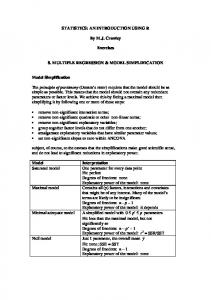
D O I T Y OURSELF G UI DE : M ULTIPLE R EGRESSION I N M INI TAB 16 Click the picture as to download the dataset used in the guide! (You will need it!)

Preliminary Information You should have read the regression for Excel handout prior to using this guide.

The Example We were given information on a book publisher in the hopes we could model the number of orders multiplied by 1000 (Num.Ordersx1000) using the number of pages in the book (Num.Pages) and number of print runs multiplied by 1000 (Print.Runsx1000). The varible Num.Ordersx1000 is the dependent or response variable. The other variables are the regressors or predictor variables. Our goal is the find a statistically significant model relating the response to the predictors. The outcome will be a regression equation along with statistical information helping us determine whether we should remain confident in the model. Step 1: Open the project file and select Stat->Regression->Regression…

Step 2: Input the variables into the regression box. Input the response and predictor variables as shown. This will tell Minitab to build the model of number of orders multiplied by 1000 (Num.Ordersx1000) using the number of pages in the book (Num.Pages) and number of print runs multiplied by 1000 (Print.Runsx1000).

Step 3: Click Graphs Select Four in one. Click OK.

Step 4: Click Options Check the ones in the following screenshot and then click OK. We’ll discuss their meanings when we read the output. So—go with the flow!

Step 5: Click Results Select the third choice because it’ll give us just enough information without flooding our screen with tons of numbers and annoying details. Click OK twice as to get the results.

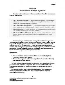
Step 6: Let’s review the Four in One! The first result is the Four-in-One residual plot. The left column contains information about the normality of the residues. Ideally you want the residues of a regression to roughly normal because it supports the ordinary least square assumptions of regression. So, we check the Q-Q and histogram and visually inspect for normality. The points hug the Q-Q line pretty well and the histogram looks roughly normal. Thus we are fairly confident the residuals are normally distributed. The top chart in the right column needs to look fairly random and scattered about zero. This condition ensures that a linear fit is good enough and that you don’t need non-linear regression. So, looking at the Four-in-One tells us the regression is looking pretty good.

Residual Plots for Num.Ordersx1000 Versus Fits 500

90

250

Residual

Percent

Normal Probability Plot 99

50 10 1 -500

-250

0 Residual

250

0 -250 -500

500

0

1000 2000 Fitted Value

Histogram

3000

Versus Order 500

Residual

Frequency

8 6 4 2 0

-400

-200

0 Residual

200

400

250 0 -250 -500

1

5

10

15 20 25 30 Observation Order

35

Step 7: Read the regression results.

Regression Analysis: Num.Ordersx1000 versus Num.Pages, Print.Runsx1000 The regression equation is Num.Ordersx1000 = - 365 + 10.3 Num.Pages + 0.183 Print.Runsx1000 Predictor Constant Num.Pages Print.Runsx1000 S = 181.988

Coef -364.85 10.2639 0.18330

SE Coef 83.08 0.5753 0.04264

R-Sq = 93.2%

PRESS = 1318339

T -4.39 17.84 4.30

P 0.000 0.000 0.000

VIF 1.195 1.195

R-Sq(adj) = 92.8%

R-Sq(pred) = 92.21%

Analysis of Variance Source Regression Residual Error Total Source Num.Pages Print.Runsx1000

DF 2 35 37 DF 1 1

SS 15771124 1159189 16930314

MS 7885562 33120

F 238.09

P 0.000

Seq SS 15159206 611918

Unusual Observations Obs 7 9 11 30 32 33

Num.Pages 249 242 114 128 120 121

Num.Ordersx1000 2630.0 2509.0 882.0 1800.0 1710.0 1715.0

Fit 2671.1 2599.3 1285.5 1407.2 1330.2 1359.2

SE Fit 97.6 94.0 40.5 42.1 40.3 42.1

Residual -41.1 -90.3 -403.5 392.8 379.8 355.8

St Resid -0.27 X -0.58 X -2.27R 2.22R 2.14R 2.01R

R denotes an observation with a large standardized residual. X denotes an observation whose X value gives it large leverage.

Minitab tells you the model:

Quick inspection shows that a one page increase in Num.Pages leads to 10.3 point increase in term on the right hand side is significant?

. How do we know if each

You can check the p-value of each coefficient and check whether each term is significant: Predictor Constant Num.Pages Print.Runsx1000

Coef -364.85 10.2639 0.18330

SE Coef 83.08 0.5753 0.04264

T -4.39 17.84 4.30

P 0.000 0.000 0.000

VIF 1.195 1.195

And we find both predictors are significant! The VIF’s are less than 10 and very close to 1.0. Thus there’s little reason to worry about multicollinearity. We can read R2 and adjusted R2 from the following line: S = 181.988

R-Sq = 93.2%

R-Sq(adj) = 92.8%

The model explains 93.2% of the variation in the data for the sample and 92.8% of the variation for the population. The ANOVA table tells whether the regression is significant: Analysis of Variance Source Regression Residual Error Total

DF 2 35 37

SS 15771124 1159189 16930314

MS 7885562 33120

F 238.09

P 0.000

The ANOVA table states the regression is significant and to expect non-zero coefficients! (Recall: The null hypothesis for regression is that all the regression coefficients are zero.) Thus we have a model worth our attention. But is there correlation as to confirm the model? Step 8: Perform the correlation for all three variables. This is part of the correlation analysis handout—you can do this part. Here are the results: Correlations: Print.Runsx1000, Num.Pages, Num.Ordersx1000 Num.Pages Num.Ordersx1000

Print.Runsx1000 0.404 0.012

Num.Pages

0.556 0.000

0.946 0.000

Cell Contents: Pearson correlation P-Value

Num.Pages is strongly correlated to Num.Ordersx1000. Print.Runsx1000 is moderately correlated to Num.Ordersx1000. The correlations are significant. Step 9: Synthesis of Findings The model was found to be significant and explained variations in the number or orders given the number of pages and number of print runs. The model of interest was a linear combination of both factors and provided an adjusted R2 explaining 92.8% of variation of the population accompanying a statistically significant p-value of 0.000. The model was supported by a significant correlation between the number of pages and number of orders, r(36) = 0.946, p = 0.000. In addition, the correlation between number of print runs and number of orders was significant, r(36) = 0.556, p = 0.000. VIF values denied concerns about multicollinearity. Thus we derived a significant model with moderate to strong correlations between the predictor and response.