These fundamental questions are answered by Theorem 4 of. Section IV, which is the ... essary theory of networks of machines, culminating with a surprisingly novel ...... Ëjordicf/gavina/BIB/reports/fmcad06 ext.pdf, 2006. [8] E. A. Lee and A.
Synchronous Elastic Networks Sava Krsti´c
Jordi Cortadella
Mike Kishinevsky, John O’Leary
Strategic CAD Labs, Intel Corporation Hillsboro, Oregon, USA
Universitat Polit`ecnica de Catalunya Barcelona, Spain
Strategic CAD Labs, Intel Corporation Hillsboro, Oregon, USA
Abstract— We formally define—at the stream transformer level—a class of synchronous circuits that tolerate any variability in the latency of their environment. We study behavioral properties of networks of such circuits and prove fundamental compositionality results. The paper contributes to bridging the gap between the theory of latency-insensitive systems and the correct implementation of efficient control structures for them.
... ...
(a)
(b)
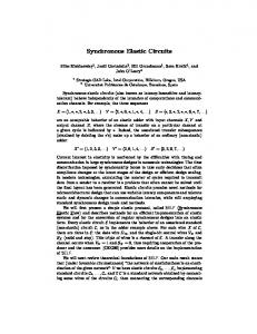
Fig. 1.
... ...
3 5 4
3 5 2 1
1
2 1
+
...
+e
... 7
7 6 2 3
4 1 0 2
6
2
3
0 2
(a) Conventional synchronous adder, (b) Synchronous elastic adder.
I. I NTRODUCTION The conventional abstract model for a synchronous circuit is a machine that reads inputs and writes outputs at every cycle. The outputs at cycle i are produced according to a calculation that depends on the inputs at cycles 0, . . . , i. Computations and data transfers are assumed to take zero delay. Latency-insensitive design by Carloni et al. [2] aims to relax this model by elasticizing the time dimension and so decoupling the cycles from the calculations of the circuit. It enables the design of circuits tolerant to any discrete variation (in the number of cycles) of the computation and communication delays. With this modular approach, the functionality of the system only depends on the functionality of its components and not on their timing characteristics. The motivation for latency-insensitive design comes from the difficulties with timing and communication in nanoscale technologies. The number of cycles required to transmit data from a sender to a receiver is governed by the distance between them, and often cannot be accurately known until the chip layout is generated late in the design process. Traditional design approaches require fixing the communication latencies up front, and these are difficult to amend when layout information finally becomes available. Elastic circuits offer a solution to this problem. In addition, their modularity promises novel methods for microarchitectural design that can use variable-latency components and tolerate static and dynamic changes in communication latencies, while—unlike asynchronous circuits—still employing standard synchronous design tools and methods. Cortadella et al. [4] present a simple elastic protocol, called SELF (Synchronous Elastic Flow) and describe methods for efficient implementation of elastic systems and for conversion of regular synchronous designs into elastic form. Inspired by the original work on latency-insensitive design [2], SELF also differs from it in ways that render the theory developed in [2] hardly applicable. In this paper we give theoretical foundations of SELF: a novel and arguably more practicable definition of elasticity, and the basic compositionality results. For space reasons, the
proofs are omitted, but are available in the technical report [7]. A. Overview Figure 1(a) depicts the timing behavior of a conventional synchronous adder that reads input and produces output data at every cycle (boxes represent cycles). In this adder, the i-th output value is produced at the i-th cycle. Figure 1(b) depicts a related behavior of an elastic adder—a synchronous circuit too—in which data transfer occurs in some cycles and not in others. We refer to the transferred data items as tokens and we say that idle cycles contain bubbles. Put succinctly, elasticization decouples cycle count from token count. In a conventional synchronous circuit, the i-th token of a wire is transmitted at the i-th cycle, whereas in a synchronous elastic circuit the i-th token is transmitted at some cycle k ≥ i. Turning a conventional synchronous adder into a synchronous elastic adder requires a communication discipline that differentiates idle from non-idle cycles (bubbles from tokens). In SELF, this is implemented by a pair of singlebit control wires: Valid and Stop. Every input or output wire Z in a synchronous component is associated to a channel in the elastic version of the same component. The channel is a triple of wires hZ, validZ , stopZ i, with Z carrying the data and the other two wires implementing the control bits, as shown in Figure 2(b). A token is transferred on this channel when validZ ∧ ¬stopZ : the sender sends valid data and the receiver is ready to accept it; see Figure 4. Additional constraints that guarantee correct elastic behavior are given in Section III. There we define precisely the class of elastic circuits and what it means for a circuit Ae to be an elastization of a given circuit A. In particular, our definition implies liveness: Ae produces infinite streams of tokens if its environment produces infinite streams of tokens at the input channels and is ready to accept infinite streams at the output channels. Suppose N is a network of standard (non-elastic) components, as in Figure 2(a). Suppose we then take elasticizations of
B
Ae
buffer
A
B
e
valid stop
C
D
D
=
channel
A
3
4
B 5
1
6
A
3
3
B 2
8
5
6
4
8
7
9
7
9
10
11
12
10
D
C
11
A
12−1
D
8−9
D
C
12
6
B B
A
D
C
2−5
A
A 4−7
e
(b)
(a)
Fig. 2.
C
e
1
2
data
10−11
Fig. 3. Four machines (left) put into a network N (middle), and the network’s dependency graph ∆(N ) (right). The nodes of ∆(N ) are wires; internal wires get two labels. The arcs are non-sequential input-output wire pairs of component circuits. Dotted arcs indicate that (1,2) and (7,10) are sequential pairs for A and C resp.; they are not part of ∆(N ) so ∆(N ) is acyclic.
A synchronous network (a) and its elastic counterpart (b).
these standard components and join their channels accordingly, as in Figure 2(b), ignoring the buffer. Will the resulting network N e be an elasticization of N ? Will it be elastic at all? These fundamental questions are answered by Theorem 4 of Section IV, which is the main result of the paper. The answers are “yes”, provided a certain graph ∆e (N e ) associated with N e is acyclic. This graph captures the information about paths inside elastic systems that contain no tokens—analogous to combinational paths in ordinary systems. Importantly, ∆e (N e ) can be constructed using only local information (the “sequentiality interfaces”) of the individual elastic components. Since elastic networks tolerate any variability in the latency of the components, empty FIFO buffers can be inserted in any channel, as shown in Figure 2(b), without changing the functional behavior of the network. This practically important fact is proved as a consequence of Theorem 4. Synchronous circuits are modeled in this paper as stream transformers, called machines. This well-known technique (see [8] and references therein) appears to be quite underdeveloped. Our rather lengthy preliminary Section II elaborates the necessary theory of networks of machines, culminating with a surprisingly novel combinational loop theorem (Theorem 1). Figure 3 illustrates Theorem 1 and, by analogy, Theorem 4 as well. It relies on the formalization of the notion of combinational dependence at the level of input-output wire pairs. Each input-output pair of a machine is either sequential or not, and the set of sequential pairs provides a machine’s “sequentiality interface”. When several machines are put together into a network N , their sequentiality interfaces define the graph ∆(N ), the acyclicity of which is a test for the network to be a legitimate machine itself. Elasticizations of ordinary circuits are not uniquely defined. On the other hand, for every elastic machine A there is a unique standard machine, denoted A| , that corresponds to it. We do not discuss any specific elasticization procedures in this paper, but state our results in the form that only involves elastic machines and their unique standard counterparts. This makes the results applicable to multiple elasticization procedures.
more complex than that of SELF (Figure 4) and consequently LID requires significantly more complex implementation. For example, conversion of a regular design into LID form needs a wrapper or registers around every module, increasing the latency of each module’s computation by two cycles—a penalty that is not required in the SELF elasticization. There might also be practical challenges in interfacing a LID system with an existing non-LID module, requiring the latter to generate stop signals with complex semantics. cycle dataZ validZ stopZ SELF LID
0 ∗ 0 0 @ @
1 A 1 0 t t
2 B 1 1
3 B 1 1
@
@
t
@
4 B 1 0
5 C 1 0
t
t
t
t
6 ∗ 0 0
7 ∗ 0 1
8 D 1 1
@
@
@
@
@
@
9 D 1 0
... ... ... ...
t
...
t
...
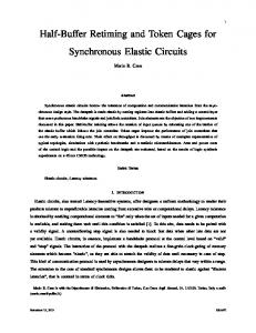
Fig. 4. Comparing the SELF and LID protocols. The bottom rows show the states of the channel Z, differentiating between bubbles (@) and tokens (t). When ¬validZ , the value at the data wire is irrelevant (labelled ∗ in cycles 0, 6 and 7). The receiver can issue a stopZ even when the sender does not send valid data (cycle 7). In the cycles 3, 4, and 9, the sender persistently maintains the same valid data as in the previous cycle. In SELF, data transfer takes place in cycles 1,4,5,9, so the transferred sequence is ABCD . . .. In LID, the same sequence of values on the channel wires signifies transfer of a different sequence of data: ABBCD . . . This is because a token is transferred on the LID channel when validZ ∧ ¬(stopZ ∧ pre(stopZ )), where pre stands for the value during the previous cycle. (The first occurrence of the stop request stopZ = 1 means “perhaps you will need to stop next cycle” and the data item B sent through the channel during cycle 2 is assumed to be successfully transmitted to the receiver.)
We emphasize that the limitations of LID implementations are not inherent to the concept of patient processes. Regarding latency properties, they do not seem to be more limited than elastic systems. Still, it turns out that patient processes are not general enough to model elastic systems as we define them in Section III. This we prove in Section V where patient processes and elastic systems are compared as alternative formalizations of latency-insensitive circuits. Suhaib et al. [12] revisited and generalized Carloni’s elasticization procedure, validating its correctness by a simulation method based on model checking. Lee et al. [9] study causality interfaces (pairwise inputoutput dependencies) and are “interested in existence and uniqueness of the behavior of feedback composition”, but do not go as far as deriving a combinational loop theorem. In their work on design of interlock pipelines [6], Jacobson et al. use a protocol equivalent to SELF, without explicitly
B. Related Work Carloni et al. [2] pioneered a theory of latency-insensitive circuits based on their notion of patient processes. Patient processes are defined at a high level of abstraction that models communication on a channel only by “token or bubble”, leaving implementation protocol(s) unspecified. In the companion paper [3], Carloni et al. give an incomplete description of an implementation protocol. Assuming our recovery of that protocol (let us call it LID) is accurate, its transfer condition is 2
Lemma 1: If f : A∞ → A∞ is contractive, then it has a unique fixpoint. Remark. One can define the distance d(a, b) between sequences a and b to be 1/2k , where k is the length of the largest common prefix of a and b. This gives the sets A∞ and Aω the structure of complete metric spaces and Lemma 1 is an instance of Banach Fixed Point Theorem. See the review paper [8] for more details and references about the metric semantics of systems and [13] for “diadic arithmetic of circuits”. We choose not to use the metric space terminology in this paper since all “metric reasoning” we need can be as easily done with equivalence relations ∼k instead. See [11] for principles of reasoning with such “converging equivalence relations” in more general contexts.
specifying it. Manohar and Martin discuss “slack elasticity” of asynchronous implementations in [10]. Their slack elasticity conditions relate to the structure of choices in the asynchronous specification. Unlike [10], in the current paper we deal with synchronous systems and we take a black box view of their control—no information about the control flow (and hence on the structure of choices) is ever used. Instead the connectivity information corresponding to the system data-flow is used for elasticization. Conservatively ignoring control flow may lead to a performance penalty, but simplifies the translation to an elastic system. II. C IRCUITS AS S TREAM F UNCTIONS In this section we introduce machines as a mathematical abstraction of circuits without combinational cycles. For simplicity, this abstraction implicitly assumes that all sequential elements inside the circuit are initialized. Extending to partially initialized systems appears to be trivial. While there is a large body of work studying circuits or equivalent objects with good (e.g. constructive [1]) combinational cycles and their composition (e.g. [5]), we deliberately restrict consideration to the fully acyclic objects, since neither logic synthesis nor timing analysis can properly treat circuits with combinational cycles. Most of the effort in this section goes into establishing modularity conditions guaranteeing that a system obtained as a network of machines (the feedback construction in particular) is a machine itself.
B. Systems Suppose W is a set of typed wires; all we know about an individual wire w is a set type(w) associated to it. A W -behavior is a function σ that associates a stream σ.w ∈ type(w)∞ to each wire w ∈ W . The set of all W -behaviors will be denoted JW K. Slightly abusing the notation, we will also write JwK for the set type(w)∞ . Notice that the equivalence relations ∼k extend naturally from streams to behaviors: σ ∼k σ 0
iff
∀w ∈ W. σ.w ∼k σ 0 .w
Notice also that a W -behavior σ can be seen as a single stream (σ[0], σ[1], . . .) of W -states, where a state is an assignment of a value in type(w) to each wire w. Definition 1: A W -system is a subset of JW K. Example. A circuit that at each clock cycle receives an integer as input and returns the sum of all previously received inputs is described by the W -system S, where W consists of two wires u, v of type Z, and S consists of all stream pairs (a, b) ∈ Z∞ × Z∞ such that b[0] = 0 and b[n] = a[0]+· · ·+a[n−1] for n > 0. Each stream pair (a, b) represents a behavior σ such that σ.u = a and σ.v = b. We will use wires as typed variables in formulas meant to describe system properties. The formulas are built using ordinary mathematical and logical notation, enhanced with temporal operators next, always, and eventually, denoted respectively by ( )+ , G, F. As an illustration, the system S in the example above is characterized by the property v = 0∧G (v + = v +u). Also, one has S |= F G (u > 0) ⇒ F G (v > 1000), where |= is used to denote that a formula is true of a system.
A. Streams A stream over A is an infinite sequence whose elements belong to the set A. The first element of a stream a is referred to by a[0], the second by a[1], etc. For example, the equation a[i] = 3i + 1 describes the stream (1, 4, 7, . . .). The set of all streams will be denoted A∞ . Occasionally we will need to consider finite sequences too; the set of all, finite or infinite, sequences over A is denoted Aω . We will write a ∼k b to indicate that the streams a and b have a common prefix of length k. The equivalence relations ∼0 , ∼1 , ∼2 , . . . are progressively finer and have trivial intersection. Thus, to prove two sequences a and b are equal, it suffices to show a ∼k b holds for every k. Note also that a ∼0 b holds for every a and b. We will use the equivalence relations ∼k to express properties of systems and machines viewed as multivariate stream functions. All these properties will be derived from the following two basic properties of single-variable stream functions f : A∞ → B ∞ .
C. Operations on Systems If W 0 ⊆ W , there is an obvious projection map σ 7→ σ ↓ W 0 : JW K → JW 0 K. These projections are all one needs for the definition of the following two basic operations on systems. Definition 2: (a) If S is a W -system and W 0 ⊆ W , then hiding W 0 in S produces a (W − W 0 )-system hideW 0 (S) defined by
causality: ∀a, b ∈ A∞ . ∀k ≥ 0. a ∼k b ⇒ f (a) ∼k f (b) contraction: ∀a, b ∈ A∞ . ∀k ≥ 0. a ∼k b ⇒ f (a) ∼k+1 f (b) Informally, f is causal if (for every a) the first k elements of f (a) are determined by the first k elements of a, and f is contractive if the first k elements of f (a) are determined by the first k − 1 elements of a.
τ ∈ hideW 0 (S) iff 3
∃σ ∈ S. τ = σ ↓ (W − W 0 ).
(b) The composition of a W1 -system S1 and a W2 -system S2 is a (W1 ∪ W2 )-system S1 t S2 defined by σ ∈ S1 t S2 iff
holds if and only if σ ∗ τ ∈ S. The causality condition for such S can be also written as follows: ∀σ, σ 0 ∈ JIK. ∀k ≥ 0. σ ∼k σ 0 ⇒ F (σ) ∼k F (σ 0 ).
σ ↓ W1 ∈ S1 ∧ σ ↓ W2 ∈ S2 .
The system in the example in Section II-B is a machine if we regard u as an input wire and v as an output wire. The same is true of the system Conn(u, v): its associated function F is the identity function.
If W and W 0 are disjoint wire sets, σ ∈ JW K, and τ ∈ JW 0 K, then there is a unique behavior ϑ ∈ JW ∪W 0 K such that σ = ϑ ↓ W and τ = ϑ ↓ W 0 . This “product” of behaviors will be written as ϑ = σ ∗ τ . (If W is the empty set, then JW K has one element—a “trivial behavior” that is also a multiplicative unit for the product operation ∗.) We will also use the notation [u 7→ a, v 7→ b, . . .] for the {u, v, . . .}-behavior σ such that σ.u = a, σ.v = b, etc. Hiding and composition suffice to define complex networks of systems. To model identification of wires, we use simple connection systems: by definition, Conn(u, v) is the {u, v}system consisting of all behaviors σ such that σ.u = σ.v. Now if S1 , . . . , Sm are given systems and u1 , . . . , un , v1 , . . . , vn are some of their wires, the network obtained from these systems by identifying each wire ui with the corresponding wire vi (of equal type) is the system
E. Feedback on Machines We will use the term feedback for the system hS | u = vi as mentioned in Section II-C when S is a machine and the wires u and v of the same type are an input and output of S respectively. Our concern now is to understand under what conditions the feedback produces a machine. To fix the notation, assume S is an (I, O)-machine given by F : JIK → JOK, with wires u ∈ I, v ∈ O of the same type A. By the note at the end of Section II-C, we have that for every σ ∈ JI − {u}K and τ ∈ JO − {v}K, σ ∗ τ ∈ hS | u = vi
if and only if
hS1 , . . . , Sm | u1 = v1 , . . . , un = vn i
∃a ∈ A∞ . F (σ ∗ [u 7→ a]) = τ ∗ [v 7→ a]),
defined as hide{u1 ,...,un ,v1 ,...,vn } (S), where
σ : A∞ → so hS | u = vi is functional when the function Fuv ∞ σ A defined by Fuv (a) = F (σ ∗ [u 7→ a]).v has a unique σ fixpoint. By Lemma 1, this is guaranteed if Fuv is contractive. The following definition introduces the key concept of sequentiality that formalizes the intutive notion that there is no combinational dependence of a given output wire on a given input wire. Sequentiality of the pair (u, v) easily implies σ contractivity of Fuv for all σ. Definition 4: The pair (u, v) is sequential for S if for every σ, σ 0 ∈ JIK and every k ≥ 0
S = S1 t · · · t Sm t Conn(u1 , v1 ) t · · · t Conn(un , vn ). The simplest case (m = n = 1) of networks is the construction hS | u = vi = hide{u,v} (S t Conn(u, v)), used for a feedback definition in Section II-E. A behavior σ belongs to hS | u = vi if and only if σ ∗ [u 7→ a, v 7→ a] ∈ S for some a ∈ JuK. D. Machines Suppose I and O are disjoint sets of wires, called inputs and outputs, correspondingly. By definition, an (I, O)-system is just an (I ∪ O)-system. Consider the following properties of an (I, O)-system S.
∧ σ.u ∼k−1 σ 0 .u
∧ ∀x ∈ I − {u}. (σ.x ∼k σ 0 .x)
⇒ F (σ).v ∼k F (σ 0 ).v
Lemma 2 (Feedback): If (u, v) is a sequential input-output pair for a machine S, then the feedback system hS | u = vi is a machine too. Example. Consider the system S with I = {u, v}, O = {w, z}, specified by equations
deterministic: ∀ω, ω 0 ∈ S. ω ↓ I = ω 0 ↓ I ⇒ ω ↓ O = ω 0 ↓ O functional: ∀σ ∈ JIK. ∃!τ ∈ JOK. σ ∗ τ ∈ S causal: ∀ω, ω 0 ∈ S. ∀k ≥ 0. ω ↓ I ∼k ω 0 ↓ I ⇒ ω ↓ O ∼k ω 0 ↓ O
w = u ⊕ ((0)#v)
z = v ⊕ v,
where all wires have type Z, the symbol ⊕ denotes the componentwise sum of streams, and # denotes concatenation. Since z does not depend on u, the pair (u, z) is sequential. The pair (v, w) is also sequential since to compute a prefix of w it suffices to know (a prefix of the same size of u and) a prefix of smaller size of v. The remaining two input-output pairs (u, w) and (v, z) are not sequential. To find the machine hS | v = wi, we need to solve the equation v = u⊕((0)#v) for v. For each u = (a0 , a1 , a2 , . . .), the equation has a unique solution v = u ˆ = (a0 , a0 + a1 , a0 + a1 +a2 , . . .). Substituting the solution into z = v⊕v, we obtain
Clearly, functionality implies determinism. Conversely, a deterministic system is functional if and only if it accepts all inputs. Note also that causality implies determinism: if ω ↓ I = ω 0 ↓ I, then ω ↓ I ∼k ω 0 ↓ I holds for every k, so ω ↓ O ∼k ω 0 ↓ O holds for every k too, so ω ↓ O = ω 0 ↓ O. Definition 3: An (I, O)-machine is an (I, O)-system that is both functional and causal. A functional system S uniquely determines and is determined by the function F : JIK → JOK such that F (σ) = τ 4
a description of hS | v = wi by a single equation that relates its input and output: z = u ˆ⊕u ˆ. The other feedback hS | u = zi is easier to calculate; it is given by equation w = v⊕v⊕((0)#v).
A. Input-output Structure, Channels, and Transfer We assume that the set of wires is partitioned into data, valid, and stop wires, so that for each data wire X there exist associated wires validX and stopX of boolean type. (In actual circuit implementations, validX and stopX need not be physical wires; it suffices that they be appropriately encoded.) Definition 5: Let I, O be disjoint sets of data wires. An [I, O]-system is an (I 0 , O0 )-machine, where I 0 = I ∪ {validX | X ∈ I} ∪ {stopY | Y ∈ O} and O0 = O ∪ {validY | Y ∈ O} ∪ {stopX | X ∈ I}. The triples hX, validX , stopX i (for X ∈ I) and hY, validY , stopY i (for Y ∈ O) are to be thought of as elastic input and output channels of the system. Let transferZ be a shorthand for validZ ∧ ¬stopZ and say that transfer along Z occurs in a state s if s |= transferZ . Given a behavior σ = (σ[0], σ[1], σ[2], . . .) of an [I, O]-system and Z ∈ I ∪ O, let σZ be the sequence (perhaps finite!) obtained from σ.Z = (σ[0].Z, σ[1].Z, σ[2].Z, . . .) by deleting all entries σ[i].Z such that transfer along Z does not occur in σ[i]. The transfer behavior σ | associated with σ is then defined by σ | .Z = σZ . If all sequences σZ are infinite, then σ | is an (I ∪ O)-behavior; in general, however, we only have σZ ∈ type(Z)ω . For each wire Z of an [I, O]-system S we introduce an auxiliary transfer counter variable tctZ of type Z. The counters serve for expressing system properties related to transfer. By definition, tctZ is equal to the number of states that precede the current state and in which transfer along Z has occurred. That is, for every behavior σ of S, we have σ.tctZ = (t0 , t1 , . . .), where tk is the number of indices i such that i < k and transfer along Z occurs in σ[i]. Note that the sequence σ.tctZ is non-decreasing and begins with t0 = 0. The notation min tctS , for any subset S of I ∪ O will be used to denote the smallest of the numbers tctZ , where Z ∈ S.
F. Networks of Machines and the Combinational Loop Theorem Consider a network N = hS1 , . . . , Sm | u1 = v1 , . . . , un = vn i, where S1 , . . . , Sm are machines with disjoint wire sets and the pairs (u1 , v1 ),. . . ,(un , vn ) involve n distinct input wires ui and n distinct output wires vi . (There is no assumption that ui , vi belong to the same machine Sj .) Our goal is to understand under what conditions the system N is a machine. Note that N = hS | u1 = v2 , . . . , un = vn i, where S = S1 t · · · t Sm . It is easy to check that an input-output pair (u, v) of S is sequential if either (1) (u, v) is sequential for some Si , or (2) u and v belong to different machines. Thus, the information about sequentiality of input-output pairs of the “parallel composition” machine S is readily available from the sequentiality information about the component machines Si , and our problem boils down to determining when a multiple feedback operation performed on a single machine results in a system that is itself a machine. Simultaneous feedback specified by a set of two or more input-output pairs of a machine does not necessarily produce a machine even if all pairs involved are sequential. Indeed, in the example in Section II-E, we had a system S with two sequential pairs (u, z) and (v, w), but (u, z) ceases to be sequential for hS | v = wi. Indeed, if z and u are related by z = u ˆ⊕u ˆ, then knowing a prefix of length k of z requires knowing the prefix of the same length of u; a shorter one would not suffice. To ensure that a multiple feedback construction produces a machine, one needs to show that, in addition to the wire pairs to be identified, sufficiently many other input-output pairs are also sequential. A precise formulation for a double feedback is given by a version of the Beki´c Lemma: for the system hS | u = w, v = zi to be a machine, it suffices that three pairs of wires be sequential—(u, w), (v, z), and one of (u, z), (v, w). This non-trivial auxiliary result is needed for the proof of Theorem 1 below, and is a special case of it. Given an (I, O)-machine S, let its dependency graph ∆(S) have the vertex set I ∪ O and directed edges that go from u to v for each pair (u, v) ∈ I × O that is not sequential. For a network system N = hS1 , . . . , Sm | u1 = v1 , . . . , un = vn i, its graph ∆(N ) is then defined as the direct sum of graphs ∆(S1 ), . . . , ∆(Sm ) with each vertex ui (1 ≤ i ≤ n) identified with the corresponding vertex vi (Figure 3). Theorem 1 (Combinational Loop Theorem): The network system N is a machine if the graph ∆(N ) is acyclic.
B. Definition of Elasticity An elastic component, when ready to communicate over an output channel must remain ready until the transfer takes place. Definition 6: The persistence conditions for an [I, O]system S are given by S |= G (validY ∧ stopY ⇒ (validY )+ ∧ Y + = Y )
(1)
for every Y ∈ O. The conjunct Y + = Y can be removed from (1) without affecting the definition of elastic machines (it follows from other conditions). The most useful consequence of persistence is the “handshake lemma”: S |= G F validY ∧ G F ¬stopY ⇒ G F transferY
III. E LASTIC M ACHINES
Liveness of an elastic component is expressed in terms of token count: if all input channels have seen k transfers and there is an output channel that has seen less, then the communication on output channels with the minimum amount of transfer must be eventually offered. The following definition formalizes this,
In this section we give the definition of elastic machines. Its four parts—input-output structure, persistence conditions, liveness conditions, and the transfer determinism condition— are covered by Definitions 5-8 below. 5
2
a
1
b
c d e
1 0 1
2
a
1
b
c d e
1 1 1
2
a
2
b
c d e
1 1 1
k transfers on the output channels in the cooperating environment. Thus, it is not surprising (even though the proof is not obvious) that the determinism postulated in Definition 8 suffices to derive the causality of S | : Theorem 2: If S is an [I, O]-elastic machine, then S | is an (I, O)-machine. In the situation of Definition 8, we say that S is an elasticization of S | and that S | is the transfer machine of S.
Fig. 5. Liveness: Only the hungriest channels (shaded) are being served. The numbers indicate the current token count at each channel.
together with a similar commitment to eventual readiness on input channels. (See also Figure 5.) Definition 7: The liveness conditions for an [I, O]-system are given by
IV. E LASTIC N ETWORKS An elastic network N is given by a set of elastic machines S1 , . . . , Sm with no shared wires, together with a set of channel pairs (X1 , Y1 ), . . . , (Xn , Yn ), where the Xi are n distinct input channels and the Yi are n distinct output channels. As a network of standard machines, the elastic network N is defined by
S |= G (min tctO = tctY ∧ min tctI > tctY ⇒ F validY )(2) S |= G (min tctI∪O = tctX ⇒ F ¬stopX ) (3) for every Y ∈ O and every X ∈ I. In practice, elastic components will satisfy simpler (but stronger) liveness properties; e.g. remove min tctO ≥ tctY from (2) and replace min tctI∪O ≥ tctX with min tctO ≥ tctX in (3). However, a composition of such components, while satisfying (2) and (3), may not satify the stronger versions of these conditions. Consider single-channel [I, O]-systems satisfying the persistence and liveness conditions: an elastic consumer is a [{Z}, ∅]-system C satisfying (4) below; similarly, an elastic producer is a [∅, {Z}]-system P satisfying (5) and (6). C |= G F ¬stopZ P |= G (validZ ∧ stopZ ⇒ (validZ )+ ) P |= G F validZ
N = hS1 , . . . , Sm | Xi = Yi , validXi = validYi , AAAAAAi stopXi = stopYi (1 ≤ i ≤ n)i for which we will use the shorter notation N = hhS1 , . . . , Sm [] X1 = Y1 , . . . , Xn = Yn ii. We will define a graph that encodes the sequentiality information about the network N and prove in Theorem 4 that acyclicity of that graph implies that N is an elastic machine | | X1 = Y1 , . . . , Xn = Yn i. and that N | = hS1| , . . . , Sm
(4) (5) (6)
A. Elastic Feedback
Let CZ be the {Z, validZ , stopZ }-system characterized by condition (4)—the largest (in the sense of behavior inclusion) of the systems satisfying this condition. Similarly, let PZ be the {Z, validZ , stopZ }-system characterized by properties (5) and (6). Finally, define the [I, O]-elastic environment to be the system F F EnvI,O = X∈I PX t Y ∈O CY .
Elastic feedback is a simple case of elastic network: hhS [] P = Qii = hS | P = Q, validP = validQ , stopP = stopQ i. Definition 9: Suppose S is an elastic machine. An inputoutput channel pair (P, Q) will be called sequential for S if � � ∧ min tctI∪O = tctQ S |= G ⇒ F validQ . (7) ∧ min tctI−{P } > tctQ
Note that EnvI,O is only a system; it is not functional and so is not a machine. When a system satisfying the persistence and liveness conditions (1-3) is coupled with a matching elastic environment, the transfer on all data wires never comes to a stall: Lemma 3 (Liveness): If S satisfies (1-3), then for every behavior ω of S t EnvI,O , all the component sequences of the transfer behavior ω | are infinite. As an immediate consequence of Liveness Lemma, if S satisfies (1-3), then
Condition (7) is a strengthening of the liveness condition (2) for channel Q. It expresses a degree of independence of the output channel Q from the input channel P ; e.g., the first token at Q need not wait for the arrival of the first token at P . This independence can be achieved in the system by storing some tokens inside, between these two channels. Note that (7) does not guarantee that connecting channels P and Q would not introduce ordinary combinational cycles. Therefore the acyclicity condition in the following theorem is required to ensure (by Theorem 1) that the elastic feedback, viewed as an ordinary network, is a machine. Theorem 3: Let S be an elastic machine and F the elastic feedback system hhS [] P = Qii. If the channel pair (P, Q) is sequential for S, then: (a) the wire pair (P, Q) is sequential for S | . If, in addition, ∆(F) is acyclic, then: (b) F is an elastic machine, and (c) F | = hS | | P = Qi.
S | = {ω | | ω ∈ S t EnvI,O } is a well-defined (I, O)-system. Definition 8: An [I, O]-system S is an [I, O]-elastic machine if it satisfies the properties (1-3) and the associated system S | is deterministic. The liveness conditions (2,3) are visibly related to causality at the transfer level: k transfers on the input channels imply 6
If ∆(N ), ∆(M), and ∆e (N ) are acyclic, then M is an elastic machine, and M| = N | . The precise relationship between graphs ∆(M) and ∆(N ) can be easily described. In practice they are at the same time acyclic or not, as a consequence of sequentiality of sufficiently many input-output wire pairs of B.
B. Main Theorems Sequentiality of two channel pairs (P, Q), (P 0 , Q) of an elastic machine does not imply their “simultaneous sequentiality” � � ∧ min tctI∪O = tctQ ⇒ F validQ . S |= G ∧ min tctI−{P,P 0 } > tctQ
V. E LASTIC VS . PATIENT S YSTEMS
This deviates from the situation with ordinary machines, where the analogous property holds and is instrumental in the proof of Combinational Loop Theorem. To justify multiple feedback on elastic machines, we have thus to postulate that simultaneous sequentiality is true where required. Specifically, we demand that elastic machines come with simultaneous sequentiality information: If S is an [I, O]elastic machine, then for every Y ∈ O a set δ(Y ) ⊆ I is given so that � � ∧ min tctI∪O = tctY ⇒ F validY . (8) S |= G ∧ min tctI−δ(Y ) > tctY
Elastic machines and patient processes of [2] provide two formalizations of the intuitive concept of latency-insensitive circuits. In this section we address their connections and differences. We begin with an overview of [2], using a minimalistic approach and terminology that differs from the original. We believe, however, that Definition 11 below matches the original definion accurately in most important aspects. A. Patient Systems The notation A∗ is for the set of finite sequences over A. A finitary W -system, by definition, is a set of behaviors σ such that σ.w is a finite sequence for every w ∈ W . A stalling stream over A is a stream over A ∪ {@}. We will refer to @ as the bubble and to elements of A as tokens. We will consider only stalling streams that contain finitely many tokens. If a is such a stream, let a ∈ A∗ denote the sequence over A obtained by dropping all bubbles from a. Clearly, a is determined by a and the sequence ∂(a) ∈ N∗ of lengths of bubble sequences between consecutive tokens of a. For example, if
Note that if P ∈ δ(Q), then the pair (P, Q) is sequential, but the converse is not implied. A function δ : O → 2I with the property (8) will be called a sequentiality interface for S. For an [I, O]-elastic machine S with a sequentiality interface δ, we define ∆e (S, δ) to be the graph with the vertex set I ∪ O and directed edges (X, Y ) where X ∈ / δ(Y ). By Theorem 3(a), ∆e (S, δ) contains ∆(S | ) as a subgraph. Given an elastic network N = hhS1 , . . . , Sm [] X1 = Y1 , . . . , Xn = Yn ii, where each Si comes equipped with a sequentiality interface δi , its graph ∆e (N ) is by definition the direct sum of graphs ∆e (S1 , δ1 ), . . . , ∆e (Sm , δm ) with each vertex Xi (1 ≤ i ≤ n) identified with the corresponding vertex Yi . Theorem 4: If the graphs ∆(N ) and ∆e (N ) are acyclic, then the network system N is an elastic machine, the cor| ¯ = hS | , . . . , Sm | X1 = responding non-elastic system N 1 | ¯ Y1 , . . . , Xn = Yn i is a machine, and N = N . As in Theorem 3, acyclicity of ∆(N ) is needed to ensure (by Theorem 1) that N defines a machine. Elasticization procedures (e.g. [4]) will typically produce elastic components with enough sequential input-output wire pairs, so that ∆(N ) will be acyclic as soon as ∆e (N ) is acyclic. Note, however, that cycles in ∆e (N ) need not correspond to combinational cycles in N seen as an ordinary network, since empty buffers with sequential elements cutting the combinational feedbacks may be inserted into N . Even though non-combinational in the ordinary sense, these cycles contain no tokens and therefore no progress along them can be made. Theorem 4 impies that insertion of empty elastic buffers does not affect the basic functionality of an elastic network, as illustrated in Figure 2(b). Definition 10: An empty elastic buffer is an elastic machine S such that S | = Conn(X, Y ) for some X, Y . Theorem 5 (Buffer Insertion Theorem): Suppose B is an empty elastic buffer with channels X, Y . Let N = hhS1 , . . . , Sm [] X1 = Y1 , . . . , Xn = Yn ii and M = hhB, S1 , . . . , Sm [] X = Y1 , X1 = Y, X2 = Y2 , . . . , Xn = Yn ii.
a = (@, @, 7, @, 4, 5, @, @, @, 8, . . .)
(9)
we have a = (7, 4, 5, 8, . . .) and ∂(a) = (2, 1, 0, 3, . . .). Two stalling streams a, b are latency equivalent, written a $ b, when a = b. Note that a $ a. By definition, a stalling W -system is a set of behaviors σ such that for every w ∈ W , σ.w is a stalling stream over type(w). Latency equivalence extends to W -behaviors and W systems: σ $ τ iff σ.w $ τ.w holds for every w ∈ W ; S $ S 0 iff for every σ ∈ S (σ ∈ S 0 ) there exists τ ∈ S 0 (τ ∈ S) such that σ $ τ . A stalling W -system S determines a standard finitary W system S | = {σ | σ ∈ S}, where σ is given by σ.w = σ.w (for all w ∈ W ). Clearly, S | $ S. Stalling the k-th token of a by d steps produces a latency equivalent stream that will be denoted stall(a, k, d). Omitting the easy definition, we give an example: if a is as in (9), then stall(a, 1, 3) = (@, @, 7, @, @, @, @, 4, 5, @, @, @, 8, . . .)
Definition 11: Let ≺ be a well-founded order1 on W and let D > 0. A patient W -system (relative to ≺ and D) is a 1 Introduction of a well-founded ordering of wires is motivated in [2] with the purpose of modeling combinational dependencies, but such dependencies in patient systems are not discussed in any detail. Moreover, the ordering of wires is implicitly assumed to be total in [2], which is somewhat unnatural. For instance, when constructing a patient adder with inputs u, v and output w, one has two ordering choices: u ≺1 v ≺1 w and v ≺2 u ≺2 w. It is not clear that a patient adder in the ≺1 -sense will be patient in the ≺2 -sense too.
7
stalling system P such that for every σ ∈ P, every u ∈ W , and every k ≥ 0 there exists σ 0 ∈ P such that (Pat-1) σ 0 .u = stall(σ.u, k, 1) and for every v 6= u there � exists dv ≤ D such that stall(σ.v, k, dv ) if u ≺ v (Pat-2) σ 0 .v = stall(σ.v, k + 1, dv ) otherwise
Are elastic machines more general? The answer is an easy “no” since, for example, the set of all possible stalling W behaviors is a patient system in the sense of Definition 11. However, if one adds to Definition 11 a reasonable requirement that a patient system be a machine, the answer is not immediately clear. Which formalization is easier to use? Without offering a definitive answer, we would argue that verifying that a lowlevel design (RTL, say) implements an elastic machine would be easier than verifying that it implements a patient system. The bottom line is that the conditions for a system to be an elastic machine are expressible as temporal properties of suitably constructed infinite-state models. This is not obvious for the determinism condition for S | in Definition 8, but can be done by replacing determinism with causality and introducing auxiliary variables for sequences of transferred values over channels. Even though (e.g., because of infinite counters involved) these conditions are not directly checkable by the existing model checking technology, there are palpable opportunities to find manageable stronger conditions that taken together imply elasticity (e.g., postulating a limit on the token count differences between channels eliminates the need for infinite counters). On the other hand, the definition of a patient system, being of the form “for every behavior σ, there exists a behavior σ 0 such that . . . ” appears to us to be intrinsically more complex. Our only positive conclusion, however, is that the mechanical checking of either of the definitions is an open problem deserving further study.
The main results of [2] can now be summarized: 1) a theorem saying that the composition of patient systems (with the same W , ≺, and D) is a patient system; 2) the definition and analysis of patient buffers, i.e. patient systems B such that B | = Connfin (u, v)—the finitary connection system; 3) a general construction that, for a given finitary system M without combinational dependencies (model of a Moore machine), produces a patient system P such that P $ M. B. Comparison The formalization given by patient systems is at a higher level of abstraction. While elastic machines deal explicitly with handshaking signals between communicating systems, patient systems communicate purely in the token/bubble language. Given an elastic (as defined in Section III) [I, O]-system E, the corresponding stalling (I ∪ O)-system E @ is obtained by projecting the finite-transfer behaviors of E to data wires and replacing data items on each wire with @ at all cycles where transfer along that wire does not occur. Precisely, let E F be the subset of E consisting of all behaviors ω such that ω | .Z is finite for all channels Z.2 Then, given ω ∈ E F , we define a stalling (I ∪ O)-behavior ω @ by � (ω.Z)[i] if (ω.validZ )[i] ∧ ¬(ω.stopZ )[i] @ (ω .Z)[i] = @ otherwise
VI. C ONCLUSION We have presented a theory of elastic machines that gives an easy-to-check condition for the compositional theorem of the form “an elasticization of a network of ordinary components is equivalent to the network of components’ elasticizations”. Verification of a particular implementation is reduced to proving that conditions of Definition 8 are satisfied for all elastic components used, and that the graph ∆e (N e ) is acyclic for every network N to which the elasticization is applied. While the definition of the graphs ∆e may appear complex because of the sequentiality interfaces involved, it should be noted that the elasticization procedures, e.g. [4], are reasonably expected to completely preserve sequentiality: a channel P belongs to δ(Q) if the wire-pair (P, Q) is sequential in the original nonelastic machine. This ensures ∆e (N e ) = ∆(N ) and so testing for sequentiality is done at the level of ordinary networks. Future work will be focused on proving correctness of particular elasticization methods, on techniques for mechanical verification of elasticity, and on extending the theory to more advanced protocols.
and finally we define the stalling system E @ as the set of all such behaviors ω @ . Clearly, the system (E @ )| is the finitary version of the standard machine E | . Now we can address some questions pertinent to the comparison of patient processes vs. elastic machines. Are patient processes more general? The answer is “no” because there exist elastic machines E such that E @ is not patient. To see this, consider an elastic machine E that starts offering new valid outputs on channel u only on even cycles. (The existence of such elastic machines is obvious.) Observe that σ.u = (@, 7, 9, . . .) is possible for some behavior σ of E @ (token 7, even though transmitted on cycle 1 was first offered on cycle 0). Then stall(σ.u, 0, 1) = (@, @, 7, 9, . . .) must also be part of a behavior of E @ , by condition (Pat-1) of Definition 11. This implies that token 9 is first offered on cycle 3, contrary to our assumption. The above example can be viewed as an indication that the condition (Pat-1) is too restrictive. It would be interesting to see if an appropriate modification of (Pat-1) results in a definition of patient processes that captures elastic machines.
Acknowledgments: Luca Carloni clarified some details of [2]. Ken McMillan pointed out several inaccuracies in a previous version of the paper and further clarified [2] for us. Gerard Berry, Ching-Tsun Chou, John Harrison, and the anonymous reviewers provided useful remarks. We are grateful for all the help we received.
2 One can prove that E is the set of all limits of behaviors of E F and so E is determined by E F .
8
R EFERENCES
[8] E. A. Lee and A. Sangiovanni-Vincentelli. A framework for comparing models of computation. IEEE Transactions on Computer-Aided Design of Integrated Circuits and Systems, 17(12):1217–1229, 1998. [9] E. A. Lee, H. Zheng, and Y. Zhou. Causality interfaces and compositional causality analysis. Invited paper in Foundations of Interface Technologies (FIT 2005), available at http://ptolemy.eecs.berkeley.edu/publications. [10] R. Manohar and A. J. Martin. Slack elasticity in concurrent computing. In Proc. 4th Int. Conf. on the Mathematics of Program Construction, volume 1422 of Lecture Notes in Computer Science, pages 272–285, 1998. [11] J. Matthews. Recursive function definition over coinductive types. In TPHOLs ’99: Proc. the 12th Int. Conf. on Theorem Proving in Higher Order Logics, pages 73–90, London, UK, 1999. Springer-Verlag. [12] S. Suhaib, D. Berner, D. Mathaikutty, J.-P. Talpin, and S. Shukla. Presentation and formal verification of a family of protocols for latency insensitive design. Technical Report 2005-02, FERMAT, Virginia Tech, 2005. [13] J. Vuillemin. On circuits and numbers. IEEE Transactions on Computers, 43(8):868–879, 1994.
[1] G. Berry. The Constructive Semantics of Pure Esterel. Draft book, available at http://www.esterel.org, version 3, July 1999. [2] L. P. Carloni, K. L. McMillan, and A. L. Sangiovanni-Vincentelli. Theory of latency-insensitive design. IEEE Transactions on ComputerAided Design of Integrated Circuits, 20(9):1059–1076, September 2001. [3] L. P. Carloni and A. L. Sangiovanni-Vincentelli. Coping with latency in SoC design. IEEE Micro, Special Issue on Systems on Chip, 22(5):12, October 2002. [4] J. Cortadella, M. Kishinevsky, and B. Grundmann. Synthesis of synchronous elastic architectures. In Proc. Digital Automation Conference (DAC), July 2006. [5] S. A. Edwards and E. A. Lee. The semantics and execution of a synchronous block-diagram language. Sci. Comput. Program., 48(1):21– 42, 2003. [6] H. M. Jacobson et al. Synchronous interlocked pipelines. In Proc. Int. Symp. on Advanced Research in Asynchronous Circuits and Systems, pages 3–12, 2002. [7] S. Krsti´c, J. Cortadella, M. Kishinevsky, and J. O’Leary. Synchronous elastic networks. Available at www.lsi.upc.edu/ ˜jordicf/gavina/BIB/reports/fmcad06 ext.pdf, 2006.
9
Lemma 4: If f : A∞ −→ A∞ is contractive and a ¯ is an arbitrary element of A∞ then the sequence of iterations f n (¯ a) (n ≥ 0) converges to the fixpoint of f .
A PPENDIX P ROOFS AND AUXILIARY R ESULTS Contents xxx xxx xxx xxx xxx xxx xxx xxx xxx xxx xxx xxx xxx xxx xxx xxx
A B C D E F G H I J K L M N O
Proof of Lemma 1 Proof of Lemma 2 Beki´c Lemma Proof of Theorem 1 Handshake Lemma Proof of Lemma 3 Preliminaries for Proof of Theorem 2 Proof of Theorem 2 Example: Strong Liveness Not Preserved by Feedback Proof of Theorem 3 (a) Proof of Theorem 3 (b) Proof of Theorem 3 (c) Sequentiality Interface for Elastic Feedback Proof of Theorem 4 Proof of Theorem 5
Remark. Lemma 1 and Lemma 4 below are well-known facts. We give their proofs for the sake of completeness. Suppose a and b are both fixpoints of f . By the contraction property, a ∼k b ⇒ a ∼k+1 b holds for every k. Since a ∼0 b, it follows that a ∼k b holds for every k, so a = b. This proves the uniqueness part. Suppose p is any finite sequence of length k and let Sp be the set of all streams a ∈ A∞ such that p is a prefix of a. It follows from the contraction condition that all streams in the set {f (a) | a ∈ Sp } have a common prefix of length k + 1. We will denote that common prefix by p† . Thus, for every p ∈ A∗ , there exists p† ∈ A∗ such that |p† | = 1 + |p| and
Proof. Let A = JuK = JvK and let H : JI − {u}K × A −→ A be given by H(σ, a) = F (σ ∗ [u 7→ a]).v. Our sequentiality assumption reads as follows:
(10)
∀σ, σ 0 , a, a0 . σ ∼k+1 σ 0 ∧a ∼k a0 ⇒ H(σ, a) ∼k+1 H(σ 0 , a0 ) (12) Starting with an arbitrary a ¯ ∈ A, define � a ¯ if n = 0 an = H(σ, an−1 ) if n ≥ 1 � a ¯ if n = 0 0 an = H(σ 0 , a0n−1 ) if n ≥ 1
(11)
Consider now the sequence �, �† , �†† , . . ., where � is the empty sequence. Since � � �† , by repeated use of (11), we obtain � � �† � �†† � · · · . Since the sequences in this chain have increasing length, there is a unique “limit” a ∈ A∞ satisfying � � �† � �†† � · · · � a. By (10), the relations � � a, �† � a, �†† � a, . . . imply �† � f (a), �†† � f (a), �††† � f (a), . . . Thus, � � �† � �†† � · · · � f (a), which forces a = f (a) (by the uniqueness of the “limit” stream), proving the existence of the fixpoint. This finishes the proof of Lemma 1.
σ Since aσ is the fixpoint of the function Fuv : a 7→ H(σ, a), we have (by Lemma 4) that aσ = lim an , and similarly aσ0 = lim a0n . By induction, it follows from (12) that aσ ∼n an and aσ0 ∼n a0n hold for every n. Also by induction, it follows from (12) that an ∼n a0n holds for all n ≤ k. Therefore, aσ ∼k aσ0 , as required.
The following fact will be used in the proof of Lemma 2. To state it, we need a definition: A sequence an of elements of A∞ (i.e. a sequence of streams over A) converges to a ∈ A∞ if every prefix of a is the prefix of all but finitely many of the an . More formally, lim an = a iff ∀n ≥ 0.∃k ≥ 0.∀m ≥ 0. m ≥ k ⇒ am
Sequentiality of the pair (u, v) implies that for every σ ∈ σ JI − {u}K there exists a unique fixpoint aσ of Fuv . (We continue with the notation from the paragraph preceding the lemma.) Consequently, F (σ∗[u 7→ a]) has the form τ ∗[v 7→ a] for a unique τ ∈ JO−{v}K. Let G : JI−{u}K −→ JO−{v}K be the function that associates τ with σ in the way just described. It is easy to verify (by definition of G) that
holds for every σ ∈ JI − {u}K, τ ∈ JO − {v}K, so it only remains to prove that G satisfies the causality condition. That in turn is a simple consequence of the causality of F and the causality of the parametrized fixpoint operator that associates aσ with σ. By the latter we mean that aσ ∼k aσ0 always follows from σ ∼k σ 0 . This we state now and prove as a separate lemma. Lemma 5: If (u, v) is a sequential pair for F , σ ∼k σ 0 , and σ0 σ , then aσ ∼k aσ0 . and Fuv aσ and aσ0 are the fixpoints of Fuv
where � stands for the prefix relation. This implies ∀p, q ∈ A∗ . p � q ⇒ p† � q † .
B. Proof of Lemma 2
σ ∗ τ ∈ hS | u = vi iff G(σ) = τ
A. Proof of Lemma 1
∀a ∈ A∞ . p � a ⇒ p† � f (a),
Proof. By Lemma 1, f has a unique fixpoint a. We prove that f m (¯ a) ∼n a holds for every m, n such that m ≥ n. (This clearly implies the lemma.) Our statement is obvious for n = 0. Arguing by induction on n, for n ≥ 1 we have f m−1 (¯ a) ∼n−1 a (induction hypothesis), so applying f to both sides and using the contraction property and f (a) = a we derive f m (¯ a) ∼n a.
C. Beki´c Lemma
[Bibliographical information. Beki´c Lemma asserts that the fixpoint of a two-variable function can be computed by iterating the fixpoint operators along the two coordinates. It ∼n a. holds in various contexts. The original result is in: Hans Beki´c, Definable operations in general algebras, and the theory of 10
1
automata and flowcharts, LNCS, vol. 177, pp. 3–35, Springer 1984.]
3
2
u =v
5
(a)
Fig. 6.
3
4 (b)
5
3
4
5
(c)
(a) Γ, (b) Γ[u=v] , (c) Γuv
0
σ σ where a and a0 are the unique fixpoints of Fuw and Fuw 0 respectively. We also added a ∼k a to the assumptions; this is justified because a ∼k a0 follows from the other assumptions by Lemma 5. We finish the proof now by deriving (13) from any of our two assumptions (i),(ii). If (i) holds, then (13) immediately follows. If (ii) holds, we first derive a ∼k+1 a0 from the assumptions of (13) and sequentiality of ({u, v}, w). Then with a ∼k+1 a0 in place of a ∼k a0 in the assumptions of (13), the conclusion c ∼k+1 c0 follows by sequentiality of (v, z).
σ ∼k+1 σ ∧ τ ∼k τ 0 ⇒ F (σ ∗ τ ).v ∼k+1 F (σ 0 ∗ τ 0 ).v.
Lemma 6: (A, v) is sequential if and only if (u, v) is sequential for every u ∈ A. Proof. The “only if” part is trivial. We prove the “if” part for the case when A has two elements. The general case is only notationally more difficult. Thus, suppose A = {x, y} and both (x, v) and (y, v) are sequential. We need to prove σ ∼k+1 σ ∧ a ∼k a0 ∧ b ∼k b0 ⇒ F (σ ∗ [x 7→ a] ∗ [y 7→ b]).v ∼k+1 F (σ 0 ∗ [x 7→ a0 ] ∗ [y 7→ b0 ]).v.
D. Proof of Theorem 1 The notation Γ[u1 =v1 ,...,un =vn ] will stand for the quotient graph obtained by identifying the vertices ui and vi (i = 1, . . . , n) in Γ. For a given directed graph Γ , a source vertex3 u of Γ , and a sink vertex v of Γ , let Γuv denote the graph obtained from Γ by: (1) removing u, v and all edges incident with them; (2) adding an edge (w, z) for all w, z such that (w, u) and (v, z) are edges of Γ . (See Figure 6.) Definition 13: If Γ and Γ0 are directed graphs such that every vertex of Γ is a vertex of Γ0 and every two vertices joined by an edge in Γ are joined by a path in Γ0 , then we say that Γ is immersed in Γ0 and write Γ ,→ Γ0 . In the main text, we used the same notation ∆ for dependency graphs of machines and systems. This is slightly ambiguous, however. For example, if S is an (I, O)-machine, then N = hS | u = vi is a system, but at the same time an (I−{u}, O−{v})-machine. When N is regarded as a network, then ∆(N ) is the quotient graph of ∆(S)[u=v] . When N is regarded as a machine, the vertex set of ∆(N ) is I∪O−{u, v}. For the proof, we need to disambiguate this notation. Definition 14: The dependency graph D(S) of an (I, O)machine S has I ∪ O as the vertex set, and {(u, v) ∈ I × O | (u, v) is not sequential for S} as its set of directed edges. The dependency graph ∆(N ) of a network N = hS1 , . . . , Sm | u1 = v1 , . . . , un = vn i is (D(S1 ) t · · · t D(Sm ))[u1 =v1 ,...,un =vn ] . Definition 15: We write N ∼ N 0 when the networks N and N 0 describe the same system. To appreciate Definition 15, note that networks are a form of system descriptions, so that, strictly speaking, a network
For the proof, just observe that both F (σ ∗[x 7→ a]∗[y 7→ b]).v and F (σ 0 ∗ [x 7→ a0 ] ∗ [y 7→ b0 ]).v are equivalent in the sense of ∼k+1 with F (σ 0 ∗ [x 7→ a0 ] ∗ [y 7→ b]).v as a consequence of the assumed sequentiality of (x, v) and (y, v). Lemma 7 (Beki´c Lemma): Suppose (u, w) and (v, z) are sequential pairs for a machine S and suppose that the four wires involved are distinct. If one of the pairs (u, z), (v, w) is also sequential, then (v, z) is sequential for hS | u = wi, (u, w) is sequential for hS | v = zi, and (therefore) the system hS | u = w, v = zi is a machine. Proof. In view of Lemma 6, it suffices to prove that (v, z) is sequential for hS | u = wi under either of the following two assumptions: (i) (u, w) and ({u, v}, z) are sequential; (ii) (v, z) and ({u, v}, w) are sequential. Thus, our goal is to prove ⇒
4
1
2
u
v
We begin with a generalization of the concept of sequentiality. Definition 12: Let S be an (I, O)-machine given by F : JIK → JOK and let A ⊆ I, v ∈ O. The pair (A, v) is sequential for S if for every k ≥ 0, every σ, σ 0 ∈ JI − AK, and every τ, τ 0 ∈ JAK one has
1
2
σ ∼k+1 σ 0 ∧ b ∼k b0 G(σ ∗ [v 7→ b]).z ∼k+1 G(σ 0 ∗ [v 7→ b0 ]).z,
where G is the function corresponding to the system hS | u = wi. We can restate this in a more convenient form σ ∼k+1 σ 0 ∧ b ∼k b0 ∧ G(σ ∗ [v 7→ b]) = τ ∗ [z 7→ c] ∧ G(σ 0 ∗ [v 7→ b0 ]) = τ ∗ [z 7→ c0 ] ⇒ c ∼k+1 c0 By definition of G, this can be further restated as σ ∼k+1 σ 0 ∧ b ∼k b0 ∧ a ∼k a0 ∧ F (σ ∗ [v 7→ b] ∗ [u 7→ a]) = τ ∗ [z 7→ c] ∗ [w 7→ a] ∧ F (σ 0 ∗ [v 7→ b0 ] ∗ [u 7→ a0 ]) = τ ∗ [z 7→ c0 ] ∗ [w 7→ a0 ] (13) ⇒ c ∼k+1 c0
3 A source vertex is a vertex with no incoming edges; a sink vertex is a vertex with no outgoing edges.
11
is not a system, although it uniquely determines one. The equivalence N ∼ N 0 implies D(N ) = D(N 0 ) but it does not imply ∆(N ) = ∆(N 0 ). Lemma 8: If u, v are vertices of Γ and if Γ ,→ Γ0 , then Γ[u=v] ,→ Γ0[u=v] . Proof. Trivial. Lemma 9: If u is a source of Γ and v is a sink of Γ, then Γuv ,→ Γ[u=v] . Proof. Easy. (Use Figure 6.) Lemma 10: If (u, v) is sequential for S, then D(hS | u = vi) ,→ D(S)[u=v] . Proof. The proof follows from D(hS | u = vi) ,→ D(S)uv and D(S)uv ,→ D(S)[u=v] . The second of these relations is an instance of Lemma 9. For the first, we prove that D(hS | u = vi) is a subgraph of D(S)uv . Notice that these graphs have a common set of vertices I ∪ O − {u, v}. Suppose (w, z) is an edge of D(hS | u = vi), i.e., (w, z) is not sequential in hS | u = vi. By Beki´c Lemma, this implies that either (w, z) is not sequential in S or that both (w, v), (u, z) are not sequential in S. In both cases, it follows that (w, z) is an edge in D(S)uv .
Proof. From (1) we obtain S |= G (validY ∧ F ¬stopY ⇒ F transferY ), which implies the lemma. F. Proof of Lemma 3 Assuming the contrary, let ω be a behavior of S t EnvI,O and let Z be a wire such that the transfer sequence ω | .Z is finite and of shortest length. This assumption implies ω |= F G min tctI∪O ≥ tctZ . If Z ∈ I, then from (3) we get ω |= G F ¬stopZ . We also have ω |= G F validZ , by (6). Since elastic producers satisfy the persistence condition, Handshake Lemma implies ω |= G F transferZ , which is a contradiction. There remains the case Z ∈ O, where we can also assume that there are no X ∈ I with ω | .X of the same length as ω | .Z. From this additional assumption we have ω |= F G (min tctI > tctZ ∧ min tctO ≥ tctZ ), so from (2) we get ω |= G F validZ . A call to consumer liveness (4) and then to Handshake Lemma yields the contradictory conclusion ω |= G F transferZ , as in the previous case. G. Preliminaries for Proof of Theorem 2 Define an elastic k-producer as a system P that satisfies the producer persistence condition (5) and the following weakened form of the producer liveness condition (6):
We strenghten now Theorem 1 as follows: If N = hS1 , . . . , Sm | u1 = v1 , . . . , un = vn i and ∆(N ) is acyclic, then N is a machine and D(N ) ,→ ∆(N ). We prove this strengthened theorem by induction on n. The case n = 0 amounts to the fact mentioned in the main text: if S1 , . . . , Sm are machines with disjoint wire sets, then S = S1 t · · · t Sm is a machine and an input-output pair (u, v) is sequential for S if either (1) (u, v) is sequential for some Si , or (2) u and v belong to different machines Si , Sj . For the induction step, let N 0 = hS1 , . . . , Sm | u1 = v1 , . . . , un−1 = vn−1 i. By induction hypothesis, N 0 is a machine, so we can write N ∼ hN 0 | un = vn i. Note that ∆(N ) = ∆(N 0 )[un =vn ] . It follows from this and the induction hypothesis D(N 0 ) ,→ ∆(N 0 ) that D(N 0 )[un =vn ] ,→ ∆(N ). This in turn, together with acyclicity of ∆(N ), implies that (un , vn ) is a sequential pair for N 0 . Thus, by Lemma 2, N is a machine. Finally, D(N )
= ,→ ,→ =
P |= G (tctZ < k ⇒ F validZ ).
(14)
Thus, a k-producer promises to cooperate in creation of at least k transfers. Similarly, we weaken the definition of the systems PZ (for any wire Z) and define PZk as the system defined by conditions (5) and (14). Then we define the k-environment (a system, but not a machine) EnvkI,O =
F
X∈I
k t PX
F
Y ∈O
CY .
The following is a finite-transfer version of Lemma 3, proved in much the same way. Note that since EnvI,O ⊆ EnvkI,O for every k, Lemma 12 actually implies Lemma 3. Lemma 12: Let S be an [I, O]-system satisfying the conditions (1-3). Then for every behavior ω ∈ S t EnvkI,O , all the component streams of the transfer behavior ω | have length at least k. Proof. The proof of Lemma 3 applies almost verbatim. The only change is that, arguing by contraction, we can now assume that, in addition to being finite, the sequence ω | .Z has length < k. Consequently, the intermediate result ω |= G F validZ is derived from (14), (6), and ω |= tctZ < k.
D(hN 0 | un = vn i) D(N 0 )[un =vn ] ∆(N 0 )[un =vn ] ∆(N ),
finishing the proof. The first immersion is justified by Lemma 10 and the second by induction hypothesis together with Lemma 8.
We will also need two easy lemmas about standard (nonelastic) machines. Lemma 13: Recall that every network
E. Handshake Lemma Persistence conditions (1) will be used through the following easily derived consequence. Lemma 11 (Handshake): If S satisfies (1), then, for every Y ∈ O,
N = hS1 , . . . , Sm | u1 = v1 , . . . , un = vn i is the system obtained by hiding the wires ui and vi in the corresponding system
S |= G F validY ∧ G F ¬stopY ⇒ G F transferY .
N ] = S1 t · · · t Sm t Conn(u1 , v1 ) t · · · t Conn(un , vn ). 12
and that W ] = W ∪ {u1 , v1 , . . . , un , vn } is the relationship between the wire sets of these systems. Suppose that the graph ∆(N ) acyclic. Then the map σ 7→ σ ↓ W : N ] → N is a bijection. In particular, if W = ∅, then N ] has exactly one behavior.
condition is vacuously true and the conjunct m < |α| can be removed from the first condition. Lemma 15: For every behavior σ ∈ PZα , the transfer sequence σ | .Z is a prefix of α. Define also the “eager consumer” machine CZ◦ (for any wire Z), characterized by the property
Proof. Consider the case n = 1. For this case, our lemma says that when S, u, v are as in Lemma 2, then for every behavior σ ∈ hS | u = vi there is a unique a ∈ JuK such that σ ∗ [u 7→ a] ∗ [v 7→ a] ∈ S. This is clear from considerations in Section II-E, notably Lemma 2. The general case follows by induction. Lemma 14: Suppose C is a machine with all input-output wire pairs sequential. Suppose also that in the network N = hC, C 0 | X1 = Y1 , . . . , Xn = Yn i exactly one wire of each pair (Xi , Yi ) is a wire of C and the other is a wire of C 0 . Then ∆(N ) is acyclic.
CZ◦ |= G ¬stopZ . For any partial I-behavior θ, define the system F F θ.X S θ = S tP θ t Y ∈O CY◦ , where P θ = X∈I PX . (17) Lemma 16: Let θ be a partial I-behavior of length k. The system S θ has exactly one behavior ω and it satisfies ω | .I = θ. Moreover, |ω | .Y | ≥ k for every Y ∈ O. Proof. It is easy to check that for finite sequences α one |α| has PZα ⊆ PZ , while for infinite α one has PZα ⊆ PZ . Consequently, if θ is a partial I-behavior of length k, we have that S θ is a subsystem of S t EnvkI,O , where we assume that | S t Env∞ I,O is just S t EnvI,O . By Lemma 12, |ω .Z| ≥ k holds for all behaviors ω of S θ and all channels Z. The eager producer and eager consumer machines have the property that their outputs depend sequentially on all their inputs. Note that S θ is of the form N ] (see Lemma 13) for a network N whose one component is S and all other components are eager producers or consumers. Repeated application of Lemma 14 proves ∆(S θ ) is acyclic. Then Lemma 13 implies that S θ has a unique behavior ω. Since ω is also a behavior of P θ , we obtain from Lemma 15 that for every input channel X the sequence ω | .X is a prefix of θ.X. Since |ω | .X| ≥ k, this implies ω | .X = θ.X for every X, which is to say that ω | .I = θ.
Proof. By assumption, the graph D(C) has no edges. Thus, ∆(N ) is the union of a bipartite graph D(C 0 ) and a set of vertices, and so is acyclic. H. Proof of Theorem 2 We will prove that S | = {ω | | ω ∈ S t EnvI,O } is causal and accepts every input stream. By assumption, the transfer determinism condition holds for S: ∀ζ, ϑ ∈ S t EnvI,O . ζ | .I = ϑ| .I ⇒ ζ | .O = ϑ| .O. (15) Let us define a partial W -behavior (for any given set W of wires) as a function θ that associates to every wire w ∈ W a (finite or infinite) sequence θ.w ∈ type(w)ω . Note that every behavior is a partial behavior as well. If all sequences θ.w (w ∈ W ) have length k, we will say that θ is a partial W behavior of length k . We allow k = ∞ in this definition, so that a partial behavior of length ∞ is just a behavior. Our main goal—the causality of S | —will be proved when we have established the following equivalent property: For every partial I-behavior θ of finite length k, there exists a partial O-behavior χ of length k such that ∀ϑ ∈ S t EnvI,O . θ � ϑ| .I ⇒ χ � ϑ| .O.
Lemma 16 implies immediately that for every θ ∈ JIK there exists ω ∈ S such that ω | .I = θ. Thus, S | accepts all inputs and it remains to prove that it satisfies the causality property (16). For this proof, we fix a partial I-behavior θ of finite length k and let ω be as provided by Lemma 16. The lemma also implies the existence of a number n such that ω[n] |= tctZ ≥ k for all channels Z. Thus, there exist a partial Obehavior χ of length k such that χ � ω | .O and
(16)
To prove this, we will need to put our system S in “eager” environments that are themselves machines, defined next. The eager environments will let us define χ as a function of θ; see (18) below. In the remainder of the proof, we will check that the so obtained χ satisfies (16). For any wire Z and a (finite or infinite) sequence α of elements of type(Z), let PZα be the “eager producer” machine that offers transfer of elements of α in order, and if it succeeds in transferring them all, then it stops offering further transfer. As a system, it is characterized by the following properties: PZα PZα
∀ζ. ζ ∼n ω ⇒ χ � ζ | .O
(18)
Suppose now ϑ ∈ S t EnvI,O satisfies θ � ϑ| .I. (This is the assumption from the causality property (16).) To finish the proof, we need to verify that χ � ϑ| .O. We will do it by exhibiting a behavior ζ ∈ S t EnvI,O such that ζ | .I = ϑ| .I and ζ ∼n ω.
(19)
In view of (15) and (18), these two properties indeed imply χ � ϑ| .O. We proceed to define a behavior ζ satisfying (19). (The definition will take more effort than the proof that it satisfies (19).)
|= G (tctZ = m ∧ m < |α| ⇒ validZ ∧ Z = α[m]) |= G (tctZ ≥ |α| ⇒ ¬validZ ∧ Z = ArbZ )
where |α| denotes the length of α and ArbZ is an arbitrary element of type(Z). Note that when α is infinite the second 13
Consider the variation PZα,k,n of the producer machine PZα , given by PZα,k,n |= G (ct ≤ n ∧ tctZ = m ∧ m < k ⇒ validZ ∧ Z = α[m])
2
a
1
b
2
a
c d e
b
1
(a)
PZα,k,n |= G (ct > n ∧ tctZ = m ⇒ validZ ∧ Z = α[m])
1 0
(b)
Fig. 7. Example demonstrating that feedback does not preserve the strong forward liveness.
where the variable ct denotes the position in the stream, i.e., for every σ ∈ S, we set σ[n] |= ct = n. The numbers k, n are arbitrary in this definition, although we will use the producers just defined with the values for k and n as defined in previous paragraphs. The sequence α is arbitrary but infinite. Intuitively, PZα,k,n eagerly offers the first k elements of α for transfer while ct ≤ n. If all k get transfered, then the machine waits until ct > n and then eagerly offers the rest of α for transfer. It is easy to see that PZα,k,n is a subsystem of PZ and that it is an elastic machine with its two outputs, dataZ , validZ depending sequentially on its input, stopZ . Moreover, for every behavior σ of this machine, one has σ | .Z � α. In particular, σ | .Z = α for every behavior σ such that σ | is infinite. Define the system F F ϑ| .X,k,n S ϑ = S t P ϑ t Y ∈O CY◦ , where P ϑ = X∈I PX .
2 0 1
a d b
c e
2 1
2 0
a d b
c
2
e 1
(a)
(b)
Fig. 8. Example demonstrating that feedback does not preserve the strong backward liveness.
hence (20) implies future progress for d: F validd . No progress on c can be guaranteed, since min tct{a,b} = tctc . To prove the strong forward liveness for F(S) = hhS [] b = eii shown in Figure 7(b) one needs to prove progress for output channels d and c, since for F(S) channel b is not an input anymore and min tctI 0 = min tct{a} = 2 > tctc . Progress on d follows immediately from progress on d in machine S. Progress on c does not. However, if we can show that the second transfer would eventually occur on the feedback channel (b, e), it would imply progress on c. By the definition of transfer and the Handshake Lemma 11 it is necessary and sufficient to demonstrate that F valide and F ¬stopb hold. The former holds due to the sequentiality of the input-output channel pair (b, e). The latter does not hold since the strong backward liveness condition for S cannot be applied until the first transfer on the output channel d occurs. Hence (20) does not hold for F(S). Note that (2) is satisfied since it only requires progress on the output channel d. Figure 8 shows an example demonstrating that feedback does not preserve the strong backward liveness either. The counter-example for the strong backward liveness is (almost) symmetric to the forward case. Figure 8(a) depicts an elastic machine S with a sequential channel pair (b, e) during a cycle when channel a has seen 2 transfers, channel d (an input channel in this example) - 0 transfers, and all other channels - 1 transfer each. For machine S:
Arguing as in the proof of Lemma 16, we obtain that S ϑ has exactly one behavior ζ and that it satisfies ζ | .I = ϑ| .I. Finally, to deduce ζ ∼n ω, note that P ϑ and P θ are machines with identical behaviors “up to ct = n”; that is, for every behavior of P ϑ there is a ∼n -equivalent behavior of P θ and vice versa. Therefore, the systems S ϑ and S θ must be in the same relationship. Since ζ, ω are the only behavors of S ϑ , S θ respectively, it follows that ζ ∼n ω. I. Example: Strong Liveness Not Preserved by Feedback The forward and backward strong liveness conditions for an [I, O]-system are given by |= G (min tctI > tctY ⇒ F validY ) |= G (min tctO ≥ tctX ⇒ F ¬stopX )
1 0
1
PZα,k,n |= G (ct ≤ n ∧ tctZ ≥ k ⇒ ¬validZ ∧ Z = ArbZ )
S S
c d e
(20) (21)
for every X ∈ I and for every Y ∈ O. In practice, elastic components satisfy these strong liveness conditions. However, a composition of such components, while satisfying weaker liveness conditions (2) and (3), may not satisfy the stronger versions (20) and (21). The fundamental difference between the liveness and the strong liveness is as follows: while the strong liveness promises progress on all under-served output (20) or input (21) channels, the liveness only guarantees progress on the least served, so to speak the “hungriest”, channels. Figure 7 shows an example demonstrating that feedback does not preserve the strong forward liveness. Figure 7(a) depicts an elastic machine S with a sequential channel pair (b, e) during a cycle when channel a has seen 2 transfers, channel d - 0 transfers, and all other channels - 1 transfer each. For machine S: min tctI = min tct{a,b} = 1 > tctd ,
min tctO = min tct{c,e} = 1 ≥ tctd = 0 hence (21) implies future progress for input d: F ¬stopd . No progress on a can be guaranteed, since min tct{c,e} < tcta . To prove the strong backward liveness for F(S) = hhS [] b = eii shown in Figure 8(b) one needs to prove progress for input channels d and a, since for F(S) channel e is not an output anymore and min tctO0 = min tct{c} = 2 ≥ tcta . Progress on d follows immediately from progress on d in machine S. If we can show that the second transfer would eventually occur on the feedback channel (b, e), it would imply 14
number n we choose now any integer such that ω[n] |= tctQ = k, and for any ϑ such that θ � ϑ| .I, we define F S ϑ = S t P ϑ t Y ∈O CY◦ ,
progress on a. By the definition of transfer and the Handshake Lemma 11 it is necessary and sufficient to show that F valide and F ¬stopb . The latter holds due to the strong backward liveness (21) of the original machine S. The former, however, does not hold since the sequentiality of channel (b, e) cannot be applied until the first transfer on the input channel d occurs. Hence (21) does not hold for F(S), while (3) holds since it only requires progress on the input channel d.
where
.P,k−1,n
t
G
|
ϑ PX
.X,k,n
.
X∈I−P
The remaining details of the derivation of χ � ϑ| .Q are now pure repetition of what is done in the proof of Theorem 2 and are therefore omitted.
J. Proof of Theorem 3 (a) This proof will use results and arguments from the proof of Theorem 2 above. Let us begin with the appropriate strengthening of Lemma 12. Lemma 17: Let F F k EnvkI,O,P = PPk−1 t X∈I−P PX t Y ∈O CY
K. Proof of Theorem 3 (b) We will prove here that hhS [] P = Qii satisfies the persistence and liveness conditions. The transfer determinism (even functionality) property follows from part (c), proved in Section L below. Let us start with notation:
and let S be an [I, O]-system satisfying the conditions (1-3) and (7). Then for every behavior ω ∈ S t EnvkI,O,P one has |ω | .Q| ≥ k.
S 0 = hhS [] P = Qii
I 0 = I − {P }
µZ = min tctI∪O ≥ tctZ
Proof. Let ω ∈ S tEnvkI,O,P . Clearly, EnvkI,O,P ⊆ Envk−1 I,O , so by Lemma 12, ω |= F G tctZ ≥ k − 1 holds for all Z ∈ I ∪ O. Assume |ω | .Q| < k, the contrary of what we are to prove. Thus, ω |= F G (min tctI∪O ≥ k − 1 ∧ tctQ = k − 1).
|
P ϑ = PPϑ
O0 = O − {Q}
µ0Z = min tctI 0 ∪O0 ≥ tctZ
Recall that for every behavior ω 0 of S 0 there exists a unique behavior ω of S such that ω.(I 0 ∪ O0 ) = ω 0 ω.P = ω.Q ω.validP = ω.validQ ω.stopP = ω.stopQ
(22)
We claim now that ω |= F G tctX ≥ k for every X ∈ I − P . To prove this claim, assume it is not true. Then we have ω |= F G (min tctO ≥ k − 1 ∧ tctX = k − 1) for some X ∈ I − P . Thus, ω |= F G min tctI∪O ≥ tctX and since ω ∈ S, the liveness of S implies ω |= G F ¬stopX . On the k , from ω |= other hand, since ω.{X, validX , stopX } ∈ PX F G tctX = k − 1 and (14) we can derive ω |= G F validX . k satisfies the persistence condition (1), Lemma 11 Since PX implies ω |= G F transferX , which contradicts our assumption ω |= F G tctX = k − 1. This finishes the proof of the claim. From (22), the claim above, and the elastic sequentiality condition (7), we obtain ω |= G F validQ . On the other hand, we have ω |= G F ¬stopQ since CQ is a component of our system. Invoking Lemma 11 again, we obtain ω |= G F transferQ , which contradicts our starting assumption |ω | .Q| < k and so finishes the proof.
(23)
Just from the observation that for each Z ∈ I 0 ∪ O0 the stream triples (ω 0 .Z, ω 0 .validZ , ω 0 .stopZ ) and (ω.Z, ω.validZ , ω.stopZ ) are equal, it follows that S 0 satisfies the persistence conditions (1). Turning to the liveness conditions, we first prove an auxiliary result. Lemma 18: Let φn = min tctI 0 > n∧min tctO0 ≥ n. Then for every n ≥ 0 and every behavior ω ∈ S as in (23), one has ω |= G (φn ⇒ F tctP > n). Proof. The proof is by induction on n. We can assume ω |= G (φn ⇒ F tctP ≥ n).
(24)
Indeed, this is trivially true for n = 0, and for n > 0 it follows from the induction hypothesis ω |= G (φn−1 ⇒ F tctP > n − 1) and the obvious fact ω |= φn ⇒ φn−1 . Arguing by contradiction, we can assume
Suppose now θ is a partial I-behavior with |θ.P | = k − 1 and |θ.X| = k for all X ∈ I − P . Define the system S θ in the eager environment by the same equation (17) used in the proof of Theorem 2. In the same way that we derived Lemma 16 from Lemma 12, Lemma 14, and Lemma 13, we can now use Lemma 17 in place of Lemma 12 and prove the following: The system S θ has a unique behavior ω, and that behavior satisfies the properties ω | .I = θ and |ω | .Q| ≥ k. Let χ be the prefix of length k of ω | .Q. For the proof that the pair (P, Q) is sequential for S | , it suffices to prove
ω |= F (φn ∧ G tctP ≤ n), which, in view of (24), can be sharpened into ω |= F (φn ∧ G tctP = n). Since ω |= G (φn ⇒ G φn ) (by monotonicity of tctZ ), this implies ω |= F G (φn ∧ tctP = n). (25) Clearly, ω |= G (φn ∧ tctP = n ⇒ µP ),
∀ϑ ∈ S t EnvI,O . θ � ϑ| .I ⇒ χ � ϑ| .Q.
which with (25) gives ω |= F G µP , which in turn, combined with (3), gives ω |= F G F ¬stopP . (26)
This can indeed be derived in the same manner we derived the similar condition (16) in the proof of Theorem 2. For the 15
Since ω |= G (µ0Y ∧ tctP > tctY ⇒ µY ), we can restate this goal as
Since ω |= G (tctP = tctQ ), we have ω |= G (φn ∧ tctP = n ⇒ µQ ∧ min tctI 0 > tctQ ),
ω |= G (G tctY = n ⇒ µ0Y ∧ ψ ⇒ F (µ0Y ∧ ψ ∧ tctP > n)).
which with (25) gives ω |= F G (µQ ∧ min tctI 0 > tctQ ), which in turn, combined with (7) gives ω |= F G F validQ .
Now we use ω |= G (G tctY = n ⇒ G (µ0Y ∧ ψ ⇔ φn )) to further rewrite our goal as
(27)
ω |= G (G tctY = n ⇒ φn ⇒ F (φn ∧ tctP > n)).
From (26) and (27), we derive ω |= (G F ¬stopP ) ∧ (G F validP ). Then by Lemma 11, we have ω |= G F transferP , which implies ω |= F tctP > n, contradicting (25). This finishes the proof of Lemma 18.
This finally follows from the already seen ω |= G (φn ⇒ G φn ) (true by monotonicity of tct) and Lemma 18. L. Proof of Theorem 3 (c)
The liveness conditions for S 0 amount to the following, to be proved for every ω as in (23). ω ω
|= G (µ0Y ∧ min tctI 0 > tctY ⇒ F validY ) |= G (µ0X ⇒ F ¬stopX )
We continue with the notation I 0 , O0 , S 0 from the previous section. We need to prove that for every ω 0 ∈ S 0 t EnvI 0 ,O0 there exists ω ∈ S t EnvI,O such that ω | .(I 0 ∪ O0 ) = ω 0| and ω | .P = ω | .Q. Indeed, we have already seen that, given ω 0 ∈ S 0 , there exists ω ∈ S such that
(28) (29)
for every X ∈ I 0 and every Y ∈ O0 . We prove the simpler property (29) first. Relying on the backward liveness of S (3), it suffices to check
ω.(I 0 ∪ O0 ) = ω 0 ω.P = ω.Q ω.validP = ω.validQ ω.stopP = ω.stopQ
ω |= G ((µ0X ⇒ F ¬stopX ) ∨ F µX ),
(see (23) above), so it only remains to prove that ω ∈ EnvI,O holds for this ω. By Part (b) of the theorem (proved in the previous section) and Lemma 3 we know that ω | .Z is infinite for every Z ∈ I 0 ∪ O0 . It follows then from Lemma 18 that the sequences ω | .P and ω | .Q are (equal and) infinite. This implies that ω.{P, validP , stopP } ∈ PP and ω.{Q, validQ , stopQ } ∈ CQ . (The persistence condition in the definition of PP is equivalent to the persistence condition for the wire Q for ω and is satisfied because ω ∈ S and Q is an output of S.) Since EnvI 0 ,O0 = EnvI,O t PP t CQ and ω 0 ∈ EnvI 0 ,O0 , we finally obtain the desired ω ∈ EnvI,O .
which is equivalent to ω |= G (µ0X ∧ G stopX ⇒ F µX ). It is easy to verify that ω |= G (G stopX ⇒ ∃n. G tctX = n), so it suffices to prove ω |= G (µ0X ∧ G tctX = n ⇒ F µX ). Since ω |= G (µX ⇔ (µ0X ∧ tctP ≥ tctX )), our goal can be restated as
M. Sequentiality Interface for Elastic Feedback
ω |= G (µ0X ∧ G tctX = n ⇒ F (µ0X ∧ tctP ≥ tctX ))
Definition 16: Given a function δ : O → 2I and M ∈ I, N ∈ O, the function δ[M =N ] : O − {N } → 2I−{M } is defined by � δ(Y ) − {M } if M ∈ δ(Y ) δ[M =N ] (Y ) = δ(Y ) ∩ δ(N ) otherwise The following formula is another characterization of δ[M =N ] . Lemma 19: For every X ∈ I − {M } and Y ∈ O − {N },
and then, in view of ω |= G (µ0X ∧ G tctX = n ⇒ G µ0X ), reduced to ω |= G (µ0X ∧ G tctX = n ⇒ F tctP ≥ n). Since ω |= G (µ0X ∧ tctX = n ⇒ φn−1 ), Lemma 18 finishes the proof. For the proof of (28), notice first that, in view of (2), it suffices to prove ω |=
G ((µ0Y
X∈ / δ[M =N ] (Y ) iff X ∈ / δ(Y ) ∨ (X ∈ / δ(N ) ∧ M ∈ / δ(Y )). Proof. Easy. Lemma 20: Suppose δ : O → 2I and P, M ∈ I and Q, N ∈ O, where P 6= M and Q 6= N . Then (δ[M =N ] )[P =Q] = (δ[P =Q] )[M =N ] .
∧ ψ ⇒ F validY ) ∨ F (µY ∧ tctP > tctY ∧ ψ)),
where ψ = min tctI 0 > tctY . This is equivalent to ω |= G ((µ0Y ∧ ψ ∧ G ¬validY ) ⇒ F (µY ∧ tctP > tctY ∧ ψ)).
Proof. Directly check that for both δ 0 = (δ[M =N ] )[P =Q] and δ 0 = (δ[P =Q] )[M =N ] one has X ∈ / δ 0 (Y ) if and only if
Since ω |= G (G ¬validY ⇒ ∃n. G tctY = n),
X ∨ (X ∨ (X
it suffices to prove ω |= G (µ0Y ∧ ψ ∧ G tctY = n ⇒ F (µY ∧ tctP > tctY ∧ ψ)). 16
Y ∨ (X N ∧M Q∧P
N ∧M Q∧P N ∧M
Y ) ∨ (X Y) Y ),
Q∧P
Y)
where, to avoid clutter, we used the notation X Y for X∈ / δ(Y ). Lemma 21: If δ is a sequentiality interface for an elastic machine S and if M ∈ δ(N ), then δ[M =N ] is a sequentiality interface for hhS [] M = N ii.
Assuming the contrary, we obtain, in a similar fashion as before, ω |= F G (θ ∧ tctQ = n ∧ ¬validQ ). for some n, where θ stands for the antecedent part of the implication in (33). Again by Lemma 18, we have
Proof. Let us start again with notation: S 0 = hhS [] M = N ii 0
δ 0 = δ[M =N ]
0
I = I−{M }
O = O−{N }
µ0Z
ω |= G (θ ∧ tctQ = n ⇒ F tctM ≥ n),
= min tctI 0 ∪O0 ≥ tctZ
For every Q ∈ O0 we need to prove
ω |= F G (θ ∧ tctQ = n ∧ ¬validQ ∧ F tctM ≥ n).
ω |= G (µ0Q ∧ min tctI 0 −δ0 (Q) > tctQ ⇒ F validQ ),
This further implies (by monotonicity of tctM )
where ω is a behavior of S that corresponds to a behavior of S 0 , i.e. ω.M = ω.N
ω.validM = ω.validN
ω |= F G (θ ∧ tctQ = n ∧ ¬validQ ∧ tctM ≥ n).
ω.stopM = ω.stopN
Now, it is clear that one of the following must hold:
Consider first the case when M ∈ δ(Q). By definition of δ 0 , we have I 0 − δ 0 (Q) = I − δ(Q) and accordingly restate our goal:
ω ω
ω |= G (µ0Q ∧ min tctI−δ(Q) > tctQ ⇒ F validQ ).
|= F G (θ ∧ tctQ = n ∧ ¬validQ ∧ tctM > n), (34) |= F G (θ ∧ tctQ = n ∧ ¬validQ ∧ tctM = n). (35)
We proceed to prove that both (34) and (35) lead to contradiction. Suppose (34) is true. Notice that
With the shorthand notation ψ = min tctI−δ(Q) > tctQ , let us assume the contrary: ω |= F (µ0Q ∧ ψ ∧ G ¬validQ ).
which, combined with the previous formula, implies
ω |= G (µ0Q ∧tctM > n∧tctQ = n ⇒ µQ ∧min tctI−δ(Q) > tctQ ),
(30)
Since ω |= G (G ¬validQ ⇒ ∃n. G tctQ = n), we have
so by combining with (8) we obtain
ω |= F (µ0Q ∧ ψ ∧ G tctQ = n)
ω |= G (µ0Q ∧ tctM > n ∧ tctQ = n ⇒ F validQ ),
for some n, and therefore ω |= F G (µ0Q ∧ ψ ∧ tctQ = n).
which (since µ0Q is a conjunct of θ) contradicts (34). Suppose (35) is true. Since ω |= tctM = tctN , we have
(31)
Note now that σ |=
G (µ0Q
ω |= G (tctM = tctQ ∧ µ0Q ⇒ µN )
∧ tctQ = n ⇒ φn−1 ),
. Since M ∈ δ(N ), we have I − δ(N ) ⊆ I 0 − δ(Q) ∩ δ(N ). With these observations, we derive
where φ is as in Lemma 18. Lemma 18 is true in the current context, so we have ω |= G (µ0Q ∧ ψ ∧ tctQ = n ⇒ F tctM ≥ n).
ω |= G (θ∧tctQ = tctM = n ⇒ µN ∧min tctI−δ(N ) > tctN ).
(32)
In view of (8), this implies
From (31) and (32), we derive ω |= F G (µ0Q ∧ ψ ∧ tctQ = n ∧ tctM ≥ n).
ω |= G (θ ∧ tctQ = tctM = n ⇒ F validN ).
This implies
(36)
Since ω |= tctM = tctN and since θ has µN as one of the conjuncts, by liveness of S (3) we also get
ω |= F G (µQ ∧ ψ) and then, in view of (8),
ω |= G (θ ∧ tctQ = tctM = n ⇒ F ¬stopM ).
ω |= F G (µQ ∧ ψ ∧ F validQ ),
Since ω |= validN = validM , from (36), (37), and (35) we get
which directly contradicts (30), finishing the first branch of the proof. 0
(37)
ω |= F G (F validN ∧ F ¬stopM )
0
Suppose now M ∈ / δ(Q). By definition of δ , we have I − δ 0 (Q) = I 0 − δ(Q) ∩ δ(N ) and our goal is
By Lemma 11 (and ω |= validM = validN ), we obtain ω |= F G transferM . Thus, ω |= F G tctM > n, contradicting (35).
ω |= G (µ0Q ∧min tctI 0 −δ(Q)∩δ(N ) > tctQ ⇒ F validQ ). (33) 17
and δN = (δN 0 )[Xn =Yn ] . Since ∆(N 0 ) has the acyclic graph ∆(N ) as a quotient, it must be acyclic too. Similarly, ∆e (N 0 ) must be acyclic as well. By induction hypothesis, N 0 is an elastic machine with a sequentility interface δN 0 , so we can write N ∼ hhN 0 [] Xn = Yn ii. We would like to use Theorem 3(b) to conclude that N is an elastic machine, but there are two conditions to check: (1) (Xn , Yn ) is a sequential channel pair for (the elastic system determined by) N 0 , and (2) ∆(hhN 0 [] Xn = Yn ii) is acyclic. For (1), it suffices to prove that Xn ∈ δN 0 (Yn ). If this were not true, there would be a path from Xn to Yn in De (N 0 , δN 0 ). By induction hypothesis, this graph is immersed in ∆e (N 0 ) so there would be a path from Xn to Yn in ∆e (N 0 ), so ∆e (N ) = ∆e (N 0 )[Xn =Yn ] would not be acyclic, which it is. This contradiction proves (1). For (2), we have the derivation
N. Proof of Theorem 4 In Section D, we disambiguated the use of the dependency symbol ∆ and now we do the same for ∆e . Definition 17: The dependency graph De (S, δ) of an elastic [I, O]-machine S with a sequentiality interface δ has the vertex set I ∪ O and a directed edge (X, Y ) for every X, Y such that X ∈ / δ(Y ). The dependency graph ∆e (N ) of an elastic network N = hhS1 , . . . , Sm [] X1 = Y1 , . . . , Xn = Yn ii is (De (S1 , δ1 ) t · · · t De (Sm , δm ))[X1 =Y1 ,...,Xn =Yn ] . Following the analogy with ordinary networks, we will write N ∼ N 0 when two elastic network determine the same elastic system. Lemma 22: Let S = S1 t · · · t Sm , where each Si is an [Ii , OSi ]-elastic machineSwith a sequentiality interface δi . Let m m I = i=1 Ii and O = i=1 Oi , and assume that theseSunions are disjoint. Define δ : O → 2I by δ(Y ) = δi (Y ) ∪ j6=i Ij for Y ∈ Oi . Then S is an [I, O]-machine, δ is a sequentiality interface for it, and De (S, δ) is the direct sum of graphs De (Si , δi ).
∆(hhN 0 [] Xn = Yn ii) = D(N 0 )[Xn =Yn ,validXn =validYn ,stopXn =stopYn ] ,→ ∆(N 0 )[Xn =Yn ,validXn =validYn ,stopXn =stopYn ] =
Proof. Straightforward checking. Lemma 23: Under the assumptions of Lemma 22, S | = | | S1 t · · · t Sm .
∆(N ),
where the immersion holds because the network N 0 is a machine (induction hypothesis) and we found in the proof of Theorem 1 that D(M) ,→ ∆(M) holds for every machine M. We have now completed the proof that N is an elastic machine. To finish the induction step, we need to check that δN is a sequentiality interface for N and that De (N , δN ) ,→ ∆e (N ). The first of these statements follows from Lemma 21 and the fact Xn ∈ δN 0 (Yn ) (proved above). For the second, we have the following derivation:
Proof. Straightforward checking. Definition 18: Given an elastic network N = hhS1 , . . . , Sm [] X1 = Y1 , . . . , Xn = Yn ii of elastic machines with disjoint inputs and outputs, let δ be as in Lemma 22, and define δN = δ[X1 =Y1 ]···[Xn =Yn ] . Remark. By Lemma 20, the order of the n operations that lead from δ to δN is irrelevant. Lemma 24: If δ is a sequentiality interface of S and X ∈ / δ(Y ), then De (hS | X = Y i, δ[X=Y ] ) ,→ De (S, δ)[u=v] .
De (N , δN )
Proof. (Mutatis mutandis, the proof is the same as that of Lemma 10.) The lemma follows from De (hS | X = Y i) ,→ De (S)XY ,→ De (S)[X=Y ] , where the second immersion is an instance of Lemma 9. For the first immersion, we prove that De (hhS [] X = Y ii) is actually a subgraph of De (S)XY . Notice that these graphs have a common set of vertices I ∪ O − {X, Y }. By Lemma 19,
= ,→ ,→ =
De (hN 0 | Xn = Yn i, (δN 0 )[Xn =Yn ] ) De (N 0 , δN 0 )[Xn =Yn ] ∆e (N 0 )[Xn =Yn ] ∆e (N ),
The first immersion here is justified by Lemma 24 and the second is justified by the induction hypothesis together with Lemma 8. We have finished the inductive proof of the claim that generalizes part of Theorem 4. It remains to prove that if N = hhS1 , . . . , Sm [] X1 = Y1 , . . . , Xn = Yn ii and both graphs | ¯ = hS | , . . . , Sm ∆(N ), ∆e (N ) are acyclic, then N | X1 = 1 | ¯ Y1 , . . . , Xn = Yn i is a machine, and N = N . Observe that Theorem 3(a) implies D(S | ) ,→ De (S, δ) for every elastic machine S and a sequentiality interface δ for it. As a consequence,
W ∈ / δ[X=Y ] (Z) iff W ∈ / δ(Z) ∨ (W ∈ / δ(Y ) ∧ X ∈ / δ(Z)) The left-hand side of this relation says that (W, Z) is an edge of De (hS | X = Y i, δ[X=Y ] ), while the right-hand side implies that (W, Z) is an edge of De (S, δ)XY . Starting the proof of Theorem 4, consider the following claim. If N = hhS1 , . . . , Sm [] X1 = Y1 , . . . , Xn = Yn ii and both graphs ∆(N ), ∆e (N ) are acyclic, then N is an elastic machine, δN is a sequential interface for it, and De (N , δN ) ,→ ∆e (N ). We prove this claim by induction on n. The case n = 0 follows immediately from Lemma 22. For the induction step, let N 0 = hhS1 , . . . , Sm [] X1 = Y1 , . . . , Xn−1 = Yn−1 ii. Note that ∆e (N ) = ∆e (N 0 )[Xn =Yn ]
¯) ∆(N | = (D(S1| ) t · · · t D(Sm ))[X1 =Y1 ,...,Xn =Yn ] e ,→ (D (S1 , δ1 ) t · · · t De (Sm , δm ))[X1 =Y1 ,...,Xn =Yn ] = ∆e (N ) ¯ ) is acyclic too, Since ∆e (N ) is acyclic, it follows that ∆(N ¯ is a machine. and then by Theorem 1 that N 18
X1
X1
X1
Y
Y1
Y1
Y1
X
Fig. 9. From left to right: the graphs ∆e (N 0 ), ∆e (N ), and ∆e (M). Shaded areas show pairs of vertices that need to be identified. The arc from X to Y should be absent if δ0 (Y ) = {X}.
¯ is proved by induction on n. Finally, the equality N | = N The case n = 0 is Lemma 23. For the induction step, we have N|
= (hhN 0 [] Xn = Yn ii)| = h(N 0 )| | Xn = Yn i = hN¯ 0 | Xn = Yn i ¯, = N
| where N¯ 0 = hS1| , . . . , Sm | X1 = Y1 , . . . , Xn−1 = Yn−1 i. The second equality here follows from Theorem 3(b), and the third follows by induction hypothesis.
O. Proof of Theorem 5 We begin with an easy lemma about ordinary machines. Lemma 25: If S is a machine with a sequential pair (X1 , Y1 ) then hS | X1 = Y1 i = hS t Conn(X, Y ) | X = Y1 , X1 = Y i. Let N 0 = hhS1 , . . . , Sm [] X2 = Y2 , . . . , Xn = Yn ii. We have ∆e (N ) = ∆e (N 0 )[X1 =Y1 ] ∆e (M) = (∆e (N 0 ) t De (B, δ0 ))[X=Y1 ,X1 =Y ] where δ0 is a sequentiality interface for B, which must be given either by δ0 (Y ) = {X} or δ0 (Y ) = ∅. A simple analysis shows that the existence of a cycle in ∆e (M) implies the existence of a cycle in ∆e (N ) (Figure 9). Theorem 4 now implies N| M|
= h(N 0 )| | X1 = Y1 i = h(N 0 )| , B | | X = Y1 , X1 = Y i
Since B | = Conn(X, Y ), Lemma 25 completes the proof of Theorem 5.
19