synthesis of asynchronous controllers for ... - Semantic Scholar

SYNTHESIS OF ASYNCHRONOUS CONTROLLERS FOR HETEROGENEOUS SYSTEMS

a dissertation submitted to the department of electrical engineering and the committee on graduate studies of stanford university in partial fulfillment of the requirements for the degree of doctor of philosophy

By Kenneth Yi Yun August 1994

c Copyright 1994 by Kenneth Yi Yun All Rights Reserved

ii

I certify that I have read this dissertation and that in my opinion it is fully adequate, in scope and in quality, as a dissertation for the degree of Doctor of Philosophy. David L. Dill (Principal Advisor)

I certify that I have read this dissertation and that in my opinion it is fully adequate, in scope and in quality, as a dissertation for the degree of Doctor of Philosophy. Teresa H.-Y. Meng

I certify that I have read this dissertation and that in my opinion it is fully adequate, in scope and in quality, as a dissertation for the degree of Doctor of Philosophy. Stephen P. Boyd

Approved for the University Committee on Graduate Studies:

iii

Abstract There are two synchronization mechanisms used in digital systems: synchronous and asynchronous. Synchronous or asynchronous refers to whether the system events occur in lock-step based on a clock or not. Today's system components typically employ the synchronous paradigm primarily because of the availability of the rich set of design tools and algorithms and, perhaps, because of the designers' perception of \ease of design" and the lack of alternatives. Even so, the interfaces among the system components do not strictly adhere to the synchronous paradigm because of the cost bene t of mixing modules operating at dierent clock rates and modules with asynchronous interfaces. This thesis addresses the problem of how to synthesize controllers operating in heterogeneous systems | systems with components employing dierent synchronization mechanisms. We introduce a new design style called extended-burst-mode. The extended-burstmode design style covers a wide spectrum of sequential circuits ranging from delayinsensitive to synchronous. We can synthesize multiple-input change asynchronous nite state machines, and many circuits that fall in the gray area between synchronous and asynchronous which are dicult or impossible to synthesize automatically using existing methods. Our implementation of extended-burst-mode machines uses standard combinational logic, generates low-latency outputs and guarantees freedom from hazards at the gate level. We present a complete set of automated sequential synthesis algorithms: hazardfree state assignment, hazard-free state minimization, and critical-race-free state encoding. We also describe two radically dierent hazard-free combinational synthesis iv

methods: two-level sums-of-products implementation and multiplexor trees implementation. Existing theories for hazard-free combinational synthesis are extended to handle non-monotonic input changes. A set of requirements for freedom from logic hazards is presented for each combinational synthesis method. Experimental data from a large set of examples are presented and compared to competing methods, whenever possible. To demonstrate the eectiveness of the design style and the synthesis tool, the design of a commercial-scale SCSI controller data path is presented. This design is functionally compatible with an existing high performance commercial chip and meets the ANSI SCSI-2 standard.

v

Acknowledgments This work would not have been possible without the help of many people. I would like to thank David Dill, my advisor, for his advice, support and encouragement for the past three years. He has taught me what I know about research in computer science and engineering. I am grateful for his patience in putting up with my inarticulate ramblings, his ability to sort out important ideas, and, most of all, his ability to instill con dence in me. I would like to thank Teresa Meng, my associate advisor, for her help and guidance. She convinced me that research in this eld is not about just proving theorems and developing algorithms but about building something real and interesting as well. I would like to thank late Professor Peterson for his support and guidance and Stephen Boyd, for rescuing me at the last minute, after Professor Peterson passed away. I would like to thank the past and present members of the ASYNC group at Stanford for the insightful discussions and criticisms. They include Peter Beerel, Jerry Burch, Bill Coates, Al Davis, Mark Dean, Nanni De Micheli, Jeremy Gunawardena, Alan Marshall, Chris Myers, Steve Nowick and Polly Siegel. Working with Bill, Alan, and Polly has been a real joy. I would like to thank them for putting up with many versions of the buggy prototype synthesis tool and actually using it to design and fabricate a working communications chip. I would like to thank Al Davis and Nanni De Micheli for their extremely helpful guidance in launching my academic career. I would especially like to thank Steve Nowick, who has been my mentor from day one and the source of many insights since then. I became fascinated with practical asynchronous circuits while working with Steve on the rst SCSI example. The vi

foundation of my research was laid by Steve's work on burst-mode machines. I am grateful for his patience in mentoring me and correcting all those ungrammatical sentences in our joint papers. I would like to thank Bill Lin and Srinivas Devadas for their ideas on BDD-based hazard-free combinational synthesis. The application of this idea to the 3D sequential synthesis has complemented my earlier work very nicely. I would like to thank the researchers in the asynchronous community world-wide for the in-depth discussions: Ivan Sutherland for the inspiring lecture on Counter ow Pipeline Processor and nice circuit examples, Luciano Lavagno for discussions on STGs, Peter Vanbekbergen for discussions on interfacing to synchronous environment, Ganesh Gopalakrishinan and Erik Brunvand for discussions on 3D synthesis and TamAnh Chu for discussions on my earlier work, just to name a few. I would like to thank the users of the 3D synthesis tool, Prabhaker Kudva of Utah, Loc Nguyen of Intel and Forrest Brewer of UCSB for their patience and comments. I would like to thank Mark Knecht and the entire SCSI group at AMD for helping me understand what it takes to build a real SCSI controller and for permitting me to discuss this example in this thesis. I would like to thank Lilian Betters for making my life easier by taking care of so many administrative matters. I would especially like to thank my parents for their love and support and for bringing me to the United States, which made all this possible. I would like to thank my brother, sisters and their signi cant ones for their friendship. I would like thank Kay and Andre for proofreading the nal draft. Finally, I am eternally grateful for all the love my wife, Minsup, has given me and for all the sacri ces she has made to support me all these years. Minsup and my children, Paul and Sara, have been the joy and inspiration in my life. Without them, this work would be meaningless. The nancial support for this research came from the Semiconductor Research Corporation, Contract nos. 91-DJ-205, 92-DJ-205 and 93-DJ-205, and from the Stanford Center for Integrated Systems, Research Thrust in Synthesis and Veri cation of Multi-Module Systems. vii

\The years of anxious searching in the dark, with their intense longing, their alternations of con dence and exhaustion and the nal emergence into the light | only those who have experienced it can understand it."

Albert Einstein.

viii

Contents Abstract

iv

Acknowledgments

vi

1 Introduction

1

1.1 Motivation : : : : : : : : : : : : : : : : : : : : : : : : : : 1.1.1 Justi cations for Asynchronous Circuits : : : : : 1.1.2 Current State of Asynchronous Controller Design 1.2 Models : : : : : : : : : : : : : : : : : : : : : : : : : : : : 1.2.1 Circuit Models : : : : : : : : : : : : : : : : : : : 1.2.2 Environment Models : : : : : : : : : : : : : : : : 1.3 Background and Related Work : : : : : : : : : : : : : : : 1.3.1 Asynchronous Data Paths : : : : : : : : : : : : : 1.3.2 Asynchronous Controllers : : : : : : : : : : : : : 1.4 Contributions of the Thesis : : : : : : : : : : : : : : : : 1.5 Overview of the Thesis : : : : : : : : : : : : : : : : : : :

2 Speci cation and Implementation

2.1 Introduction : : : : : : : : : : : : : : : : : : : : : : 2.2 Controller Speci cation : : : : : : : : : : : : : : : : 2.2.1 Formal De nition of Extended-Burst-Mode : 2.3 Implementation Overview : : : : : : : : : : : : : : 2.3.1 A Simple Example : : : : : : : : : : : : : : 2.4 3D Machine Operation : : : : : : : : : : : : : : : : ix

: : : : : :

: : : : : :

: : : : : :

: : : : : : : : : : : : : : : : :

: : : : : : : : : : : : : : : : :

: : : : : : : : : : : : : : : : :

: : : : : : : : : : : : : : : : :

: : : : : : : : : : : : : : : : :

: : : : : : : : : : : : : : : : :

: : : : : : : : : : : : : : : : :

1 2 3 4 5 5 6 7 8 15 16

18 18 19 22 24 25 29

3 Hazard Considerations

3.1 Introduction : : : : : : : : : : : : : : : : : : 3.2 Sequential Hazard : : : : : : : : : : : : : : : 3.2.1 Essential Hazard : : : : : : : : : : : 3.2.2 Environmental Constraints : : : : : : 3.2.3 Summary : : : : : : : : : : : : : : : 3.3 Function Hazard : : : : : : : : : : : : : : : 3.3.1 De nitions : : : : : : : : : : : : : : : 3.3.2 Generalized Transition : : : : : : : : 3.3.3 Extended-Burst-Mode Transition : : 3.3.4 Critical Race : : : : : : : : : : : : : 3.4 Combinational Logic Hazards : : : : : : : : 3.4.1 Two-Level AND-OR Implementation 3.4.2 BDD Implementation : : : : : : : : : 3.4.3 Summary : : : : : : : : : : : : : : :

4 Automatic Synthesis Procedure

: : : : : : : : : : : : : :

: : : : : : : : : : : : : :

: : : : : : : : : : : : : :

: : : : : : : : : : : : : :

: : : : : : : : : : : : : :

: : : : : : : : : : : : : :

: : : : : : : : : : : : : :

: : : : : : : : : : : : : :

: : : : : : : : : : : : : :

: : : : : : : : : : : : : :

: : : : : : : : : : : : : :

: : : : : : : : : : : : : :

4.1 Next State Assignment : : : : : : : : : : : : : : : : : : : : : : : : 4.1.1 Next State Assignment for Two-Level AND-OR : : : : : : 4.1.2 Next State Assignment for BDD-Based Multi-Level Circuit 4.2 Layer Minimization : : : : : : : : : : : : : : : : : : : : : : : : : : 4.2.1 De nitions : : : : : : : : : : : : : : : : : : : : : : : : : : : 4.2.2 Layer Minimization Algorithm : : : : : : : : : : : : : : : : 4.3 Layer Encoding : : : : : : : : : : : : : : : : : : : : : : : : : : : : 4.3.1 Layer Diagram : : : : : : : : : : : : : : : : : : : : : : : : 4.3.2 Layer Encoding Algorithm : : : : : : : : : : : : : : : : : : 4.4 Combinational Logic Synthesis : : : : : : : : : : : : : : : : : : : : 4.4.1 Two-Level AND-OR Implementation : : : : : : : : : : : : 4.4.2 BDD-Based Multi-Level Implementation : : : : : : : : : : 4.5 Experimental Results : : : : : : : : : : : : : : : : : : : : : : : : : 4.5.1 Examples Using Two-Level Synthesis : : : : : : : : : : : : x

: : : : : : : : : : : : : : : : : : : : : : : : : : : :

: : : : : : : : : : : : : : : : : : : : : : : : : : : :

32 32 34 34 37 38 38 39 40 42 46 46 48 53 61

63 64 70 77 80 80 84 88 88 92 95 95 95 96 97

4.5.2 Comparison to Locally-Clocked Methods : : : : : : : : : : : : 4.5.3 Experimental Results Using BDD Synthesis : : : : : : : : : :

5 Design Example: SCSI Controller

5.1 Overview : : : : : : : : : : : : : : 5.2 Implementation : : : : : : : : : : 5.2.1 BIU (Bus Interface Unit) : 5.2.2 FIFO : : : : : : : : : : : : 5.2.3 SCSI Bus Interface : : : : 5.3 Results : : : : : : : : : : : : : : :

: : : : : :

: : : : : :

: : : : : :

: : : : : :

: : : : : :

: : : : : :

: : : : : :

: : : : : :

: : : : : :

: : : : : :

: : : : : :

: : : : : :

: : : : : :

: : : : : :

: : : : : :

: : : : : :

: : : : : :

: : : : : :

: : : : : :

: : : : : :

97 99

102

102 106 107 111 113 115

6 Conclusion

117

Bibliography

120

6.1 Summary : : : : : : : : : : : : : : : : : : : : : : : : : : : : : : : : : 117 6.2 Future Work : : : : : : : : : : : : : : : : : : : : : : : : : : : : : : : : 118

xi

List of Tables 3.1 Trigger/non-trigger signal. : : : : : : : : : : : : : : : : : : : : : : : :

62

4.1 Experimental results. : : : : : : : : : : : : : : : : : : : : : : : : : : : 98 4.2 Comparisons to locally-clocked machine. : : : : : : : : : : : : : : : : 99 4.3 Comparing two-level vs BDD. : : : : : : : : : : : : : : : : : : : : : : 101

xii

List of Figures 1.1 Circuit model. : : : : : : : : : : : : : : : : : : : : : : : : : : : : : : : 1.2 AFSM implementations. : : : : : : : : : : : : : : : : : : : : : : : : :

5 13

2.1 2.2 2.3 2.4 2.5 2.6 2.7 2.8 2.9 2.10

Extended-burst-mode speci cation. : : : : : : : : : : : : Distinguishability constraints. : : : : : : : : : : : : : : : Example (unique entry condition). : : : : : : : : : : : : 3D asynchronous state machine. : : : : : : : : : : : : : : Simple example. : : : : : : : : : : : : : : : : : : : : : : : Simple example (next-state table before layer encoding). Simple example (next-state table after layer encoding). : Simple example (Karnaugh map for Y). : : : : : : : : : : Simple example (3D implementation). : : : : : : : : : : : 3D machine cycles (Types I and III). : : : : : : : : : : :

: : : : : : : : : :

: : : : : : : : : :

: : : : : : : : : :

: : : : : : : : : :

: : : : : : : : : :

: : : : : : : : : :

: : : : : : : : : :

19 22 23 25 26 27 28 28 29 30

3.1 3.2 3.3 3.4 3.5 3.6 3.7 3.8 3.9

Combinational view of the 3D state machine. : : : Essential hazard. : : : : : : : : : : : : : : : : : : Timing requirements for minimum feedback delay. Generalized transitions. : : : : : : : : : : : : : : : Critical race. : : : : : : : : : : : : : : : : : : : : Delay model. : : : : : : : : : : : : : : : : : : : : Delay model used in 3D synthesis. : : : : : : : : : Simple example (required cubes). : : : : : : : : : Illegal intersection of privileged cube. : : : : : : :

: : : : : : : : :

: : : : : : : : :

: : : : : : : : :

: : : : : : : : :

: : : : : : : : :

: : : : : : : : :

: : : : : : : : :

33 35 36 43 45 46 47 51 52

xiii

: : : : : : : : :

: : : : : : : : :

: : : : : : : : :

: : : : : : : : :

3.10 (a) BDD (b) MUX network derived from BDD (c) Simpli ed network (by constant propagation). : : : : : : : : : : : : : : : : : : : : : : : : 3.11 A CMOS multiplexor. : : : : : : : : : : : : : : : : : : : : : : : : : : 3.12 Simple example (BDD representations of X ). : : : : : : : : : : : : : : 3.13 Dynamic hazard in BDD-based implementation. : : : : : : : : : : : : 4.1 4.2 4.3 4.4 4.5 4.6 4.7 4.8 4.9 4.10 4.11 4.12 4.13 4.14 4.15

Next state assignment. : : : : : : : : : : : : : : : Conditional input setup transition. : : : : : : : : Example 2 (synchronous implementation). : : : : Example 2 (speci cation and next-state table). : : Example 2 (problem). : : : : : : : : : : : : : : : : Example 2 (solution { state graph). : : : : : : : : Example 2 (solution { next-state table). : : : : : Example 2 (circuit and timing). : : : : : : : : : : Satisfying variable ordering locally. : : : : : : : : Output-compatible but not SOP-dhf-compatible. Output-compatible but not BDD-dhf-compatible. ISEND speci cation and layer assignment. : : : : Compatibility table. : : : : : : : : : : : : : : : : Layer encoding example. : : : : : : : : : : : : : : Layer diagram. : : : : : : : : : : : : : : : : : : :

: : : : : : : : : : : : : : :

: : : : : : : : : : : : : : :

: : : : : : : : : : : : : : :

: : : : : : : : : : : : : : :

64 65 72 72 73 74 75 77 79 81 83 86 86 90 91

5.1 5.2 5.3 5.4 5.5 5.6 5.7 5.8

A simple con guration of SCSI bus. : : : : : : : : : : : : : : : : SCSI controller block diagram. : : : : : : : : : : : : : : : : : : : SCSI controller data path. : : : : : : : : : : : : : : : : : : : : : DMA protocol. : : : : : : : : : : : : : : : : : : : : : : : : : : : BIU (data transfer from DMA to FIFO). : : : : : : : : : : : : : FIFO cell (data transfer from DMA to SCSI). : : : : : : : : : : SCSI Bus Interface (initiator data transfer from FIFO to SCSI). SCSI controller design ow. : : : : : : : : : : : : : : : : : : : :

: : : : : : : :

: : : : : : : :

: : : : : : : :

103 104 105 107 109 112 114 116

xiv

: : : : : : : : : : : : : : :

: : : : : : : : : : : : : : :

: : : : : : : : : : : : : : :

: : : : : : : : : : : : : : :

: : : : : : : : : : : : : : :

: : : : : : : : : : : : : : :

: : : : : : : : : : : : : : :

54 55 56 57

Chapter 1 Introduction 1.1 Motivation Asynchronous circuits are sequential circuits which do not require external clocks to coordinate their internal operations. Asynchronous circuits were used in the earliest computers, and the research in asynchronous circuits and systems blossomed in the 1960's. However, the interests in asynchronous circuits declined in the 1970's, as synchronous circuits which use external clocks to schedule all their operations became popular, and all but vanished by the early 1980's. The main reason for the decline was the diculty of designing custom components and the amount of details with which designers had to cope. Synchronous designs oered simplicity: the only rule which designers had to be concerned about was that circuits be stable some prescribed time before and after each clock tick. Nevertheless, as VLSI technology evolved, the limitations of synchronous circuits began to surface. Some of the notable problems are clock skew, power dissipation, and interfacing to the environment. Synchronous designs have to cope with clock skew problems: the dierence in arrival times of a clock signal at various parts of a chip or a system eectively reduces the amount of time alloted for useful computation. As the feature size of VLSI chips shrank, the transistors switched faster but the distance electrons had to travel to deliver clock edges remained constant. In addition, the width of wires shrank but 1

CHAPTER 1. INTRODUCTION

2

not the vertical thickness, which meant it took even longer for electrons to travel the same distance. So the advances in VLSI technology actually aggravated clock skew problems. In order to minimize these eects, increasingly larger portions of the synchronous VLSI chips are devoted to clock distribution. It was reported that DEC's new RISC chip Alpha 21064 [19, 21] uses one third of its chip area for clock distribution. Furthermore, as more and more transistors were packed into a single chip, designers began to face real power dissipation problems. In synchronous chips with global clocking, even the inactive parts of the chip, including the clocks to those parts, dissipate power. Finally, most VLSI chips and virtually all digital systems have to interface to signals that are asynchronous. It is absurd to even try to imagine two computer systems connected via a network synchronized with a common global clock. A synchronous chip or system that interfaces to an environment which does not share a common clock must synchronize asynchronous external inputs to its own internal clock. This introduces an inherent risk of synchronization failure [12, 44]. When the digital circuits operated at relatively low speed, the probability of synchronization failure was extremely low; however, when the computer systems started using a clock rate in access of 75MHz, the probability of failure became signi cant enough to warrant a search for a new solution.

1.1.1 Justi cations for Asynchronous Circuits There are many bene ts asynchronous circuits can bring to system designs. We consider the necessity of asynchronous circuits in the systems context:

Many interface signaling protocols, such as the SCSI bus data transfer protocol, are asynchronous. Synchronous controller design would require synchronizing asynchronous handshaking signals to a high speed internal clock, complicating the design and potentially sacri cing performance.

Asynchronous circuits are ideal for building modular components. Modularity is an attractive feature in any system, because it makes global timing veri cation


3

unnecessary. Asynchronous circuits designed for high performance applications work just as well when the system speed is lowered. For example, an asynchronous module designed for a desktop workstation works equally well when placed in a laptop computer with the same architecture operating at much lower speed.

Asynchronous circuits tend to dissipate less power than synchronous counter-

parts for certain applications using CMOS technology. Asynchronous circuits have no power dissipation due to clock transitions and glitches, because CMOS circuits dissipate power only while switching. Furthermore, the data-driven nature of asynchronous circuits is ideal for low power applications that require quick transitions from standby to active, because inactive parts of the asynchronous circuits are always in \hot" standby mode without dissipating power. With the growing emphasis on portable electronics and wireless applications, low power may become a driving requirement for many new VLSI chip designs.

Asynchronous circuits have low latency output because outputs are generated

immediately upon receipt of enabling inputs, without having to wait for the next clock tick. Low latency outputs are useful in memory controllers and high speed switching networks.

1.1.2 Current State of Asynchronous Controller Design Although we made strong claims for the necessity of asynchronous circuits in the last subsection, there are several problems with asynchronous design in its current state. Asynchronous circuits are dicult to design manually, mainly because of the phenomenon called hazard | potential glitches, or undesired pulses, in the circuit. In synchronous circuits, glitches in combinational circuits do not cause problems as long as the combinational circuits stabilize before the next clock tick. However, in asynchronous circuits, no amount of glitches can be tolerated because the circuits are sensitive to every input change. Therefore, designers need to pay close attention to whether each synthesis step introduces hazards in the nal design.


4

An even greater hurdle for asynchronous design is that most existing design methodologies are either not powerful enough or too dicult to use, and, in some cases, may not even produce correct results. The machines that were popular in the 1960's, such as single-input change Human-mode machines [30, 69], are inadequate for today's design requirements. Describing asynchronous circuits using system modeling languages, such as Petri nets [56], is too complex for large machines. Because these languages were designed primarily for modeling, not every speci able machine is implementable. Most importantly, for the foreseeable future, practically every asynchronous design must interface to existing synchronous designs. Current asynchronous design methodologies are not adequate for designing controllers that are to be used in heterogeneous systems | systems which consist of both synchronous and asynchronous components. This thesis addresses all of these issues: automation, correct design methodology, simple user-level speci cation formalism, and capability to interface to synchronous designs.

1.2 Models Results produced by synthesis methods are only as good as the models used to approximate the physical circuits. If the circuit model used by a synthesis method is too optimistic, then the synthesized circuits may be incorrect, although the circuits function correctly according to the model. On the other hand, if the circuit model is too pessimistic, then the synthesized circuits may be very robust but suboptimal. In this thesis, we attempt to strike a balance between optimistic and pessimistic models so that our models represent the current generation of technology accurately. However, in some cases, we use a pessimistic model to make the analyses to guarantee the correct results more manageable.


5

1.2.1 Circuit Models A gate is a circuit component which computes the value of a logic function instantaneously, then asserts the computed value on its output after some delay. For example, an AND gate asserts the boolean product of its inputs after some delay. A gate output is connected to gate inputs by wires. A logic circuit (see gure 1.1) consists only of gates and wires; it is connected to its environment via wires. A wire transports the value of a gate output to an input of a gate or to the environment of the circuit after some delay. 1

circuit w1

environment

w2 g1

w6

w3

g gates w wires

w4 g2

g3

environment

w5

Figure 1.1: Circuit model. A change of a gate input is said to enable the gate output if the input change alters the value of the associated logic function. A gate is said to be stable if the value of the associated logic function is the same as the asserted output value. A wire is said to be stable if the value of the gate input it is connected to is the same as that of the gate output to which it is connected. A logic circuit is said to be stable if every gate and every wire in the circuit is stable.

1.2.2 Environment Models The environment of a circuit is said to operate in fundamental mode if it changes inputs to the circuit only after the circuit is stable. The environment of a circuit is said to operate in multiple-input change fundamental mode if it changes a speci ed We assume that gate outputs cannot be connected other gate outputs to simplify our circuit model, although, in some data paths, tri-state outputs and open-drain outputs can be connected to other tri-state outputs and open-drain outputs. 1


6

set of inputs to the circuit and waits for a speci ed set of outputs to change and for the circuit to stabilize before it changes the next set of inputs. The synthesis method presented in this thesis assumes a variation of the multiple-input change fundamental mode operation: The environment is allowed to change certain inputs that do not cause the outputs of the circuit to change before the circuit has stabilized. The discussion on this variation is presented in detail in section 2.1.

1.3 Background and Related Work A conventional way of classifying asynchronous circuits is by the robustness of each class of circuits with respect to delay variations of physical components in the system. Each class of circuits makes certain assumptions about delays. These assumptions directly aect the validity of synthesis methods. For example, a circuit model that assumes that gates have arbitrary delays would not be suitable for synchronous circuit synthesis, because in that model there is no guarantee that gate outputs enabled to change will stabilize within a clock period. A delay-insensitive (DI) circuit is an asynchronous circuit which operates correctly regardless of wire delay variations. In other words, the DI circuit model assumes the unbounded wire delays, that is, both gates and wires are assumed to have arbitrary nite delays. A delay-insensitive circuit consists of macromodules and the wires that connect them. Each macromodule must be designed so that delay variations on the wires do not cause malfunction of the circuit. Early work on macromodules was done by Molnar et al [46]. Since the internal design of each module assumes certain timing bounds, the internals of the circuits are not really delay-insensitive, but the communications among modules. There is a large body of theoretical work in this area, beginning with Udding and others [68, 22, 62]. A speed-independent (SI) circuit is an asynchronous circuit which operates correctly regardless of gate delay variations. Wire forks, or points of multiple fanouts, such as the junction of w and w in gure 1.1, are assumed to be isochronic. That is, changes of a gate output with multiple fanouts are assumed to arrive at the gate inputs it drives at the same time. In eect, wire delays can be lumped into gate 2

3


7

delays, that is, gates are assumed to have arbitrary nite delays but wires have zero delays | the unbounded gate delay assumption. The speed-independent assumption was viable during the early days of VLSI, when the wires within a chip had negligible delays compared to gate delays. However, in the current generation of VLSI technology, in which wire delays are no longer insigni cant, circuits designed with the SI assumption require careful layout and routing to ensure that the isochronic fork assumption is not violated. Many synthesis methods use SI circuits as target implementations [13, 45, 2, 71]. There have been some practical designs using SI circuits as well [41, 42]. There is a wide spectrum of circuits that are not SI circuits. Clearly, synchronous circuits are not speed-independent. All variations of Human-mode machines [30, 69] fall outside of the SI category. In fact, we claim that the robustness of the circuit really depends on how localized the delay variations are. There is no need to make a sweeping assumption that every gate can have a delay between 0 and 1. Nor is it safe to assume that a wire that stretches from one corner of the chip to the other has a zero delay. The synthesis method in this thesis assumes the unbounded wire delays in combinational circuits used as building blocks of sequential circuits and the bounded wire delays in sequential circuits constructed by feeding back outputs of the combinational circuits. Below, we will brie y survey current thoughts on asynchronous data path design and various asynchronous controller design styles. Although this thesis is about designing asynchronous controllers, we discuss the asynchronous data paths here brie y, partly to show just what kind of mechanisms the asynchronous controllers we design actually controls and partly to provide some background for the design example in chapter 5.

1.3.1 Asynchronous Data Paths Although it is possible to construct a chip or a module which performs nothing but control tasks, it is dicult to conceive a system that do not contain some sort of data path. The purpose of a data path is to move the data both physically and logically, either as is or after performing some operations on it. A data path is controlled by a


8

controller or a group of controllers. Conventional synchronous data paths are pipelines. Each stage of a pipeline consists of some combinational logic or wires followed by a register to store the data. A pipeline is normally controlled by a clock. In contrast, there are two radically dierent ways to design asynchronous data paths. The rst method, called micropipeline [65], was introduced by Ivan Sutherland. A micropipeline without its control circuits is identical to a synchronous pipeline with all clocks removed. Each stage of a micropipeline uses a request wire, instead of a clock edge, to signal the next stage that the data is valid. The next stage, when it receives the data, uses an acknowledge wire to signal the sender that it has received the data. The sender is not to remove the data until it receives an acknowledge signal from the receiver. This method is attractive because of its simplicity, albeit some concerns about its robustness. Speci cally, designers must take steps to assure that valid data arrive at the receiver before the accompanying request signals, which generally implies that carefully measured delays have to be added to the request wires. The SCSI controller example in chapter 5 uses a variation of the micropipeline for its data path. The second method is based on generating a completion signal in a truly self-timed way. Each data bit is encoded in 2 wires, 01 for logic 0, 10 for for logic 1, for example. Before the computation, both wires are 0. When the computation is complete, one of the wires becomes 1. When one wire of every data bit changes to 1, the sender generates a completion signal to the receiver. When the receiver acknowledges the receipt of data, the sender resets all data bits to 00. Disadvantages of this method are the large overhead in area for the dual-rail logic and the extra energy cost associated with toggling wires of the data bits whose logic values do not change.

1.3.2 Asynchronous Controllers This thesis is concerned with designing correct and ecient asynchronous controllers. There are three factors that aect the quality of the nal design and the scope of its applications: speci cation method, target implementation, and synthesis method. The design style is a general term which refers to a combination of all of these.


9

Given a design style for controllers, there are two questions one must ask: \Can the signaling and timing constraints of most controllers be described in this design style?" and \Can every legal speci cation in this design style be implemented eciently and correctly by automatic synthesis tools?" Clearly, maximizing expressiveness and maximizing implementability are con icting goals. Answers to the rst question can only be found empirically, by examining the design examples in the target application area. For example, the speci cation formalism in our design style was extended from earlier ones after consideration of the HP Post Oce packet routing chip [17], and industry-standard backplane and local bus controllers. It is the author's view, after having designed and analyzed a large number of controllers, that mechanisms to handle a moderate degree of concurrency and mechanisms to select alternative responses based on conditional signal levels as well as signal edges are essential. Fine-grained concurrency is not necessary in most applications. The correctness part of the answer to the second question can only be demonstrated reasonably by proving that the synthesis procedure guarantees that the resulting circuits observe the constraints on behavior described in the speci cations. The eciency part of the answer can only be found by performing a large number of experiments and examining the results. There have been a number of asynchronous controller design styles in the past 30 years. Many are based on high-level languages of concurrency [40, 7, 11, 22, 1] or Petri nets [13, 45, 34, 47, 71, 2, 48, 73]. These methods have proved successful for small, highly concurrent designs. However, they often lack exibility in minimization and encoding of state and in the implementation of logic functions, and thus have diculty taking advantage of global optimization techniques. Target implementations for almost all of these methods are either DI or SI circuits. Other methods based on asynchronous state machine speci cations make more realistic delay assumptions and have been implemented in numerous styles [49, 33, 59, 69]. However, these methods often allow only single-input changes or restricted multiple-input changes which impose timing constraints on inputs [69, 14, 28]. None of the currently known methods are capable of correctly implementing synchronous features.


10

We will brie y survey existing design styles and zero in on a design style called burst-mode, which has a reasonable combination of expressiveness and implementability, and present a design style that extends burst-mode by allowing more concurrency and by adding a synchronous-like feature. We call this style, extended-burst-mode.

Compilation from High-Level Languages of Concurrency Several design styles use high-level languages of concurrency as their user-level speci cation formalisms. The synthesis procedures typically consist of a series of transformations to generate either DI or SI circuits. Martin's method [39] uses Hoare's CSP (Communicating Sequential Processes) [29] as the speci cation formalism. A speci cation describes a set of concurrent processes that communicate via commands on channels. The speci cation is translated into a set of operators called production rules, which are mapped to hardware components. The resulting circuit is speed-independent. Burns [10] developed an automatic synthesis and performance analysis method for this design style. This method has been applied to a number of practical examples [38, 41, 42, 66]. Ebergen [22] uses a language derived from trace theory [58], developed by Rem, Snepscheut, and Udding. A speci cation in this language describes a sequence of events. The speci cation is decomposed into a network of macromodules; the resulting circuit is delay-insensitive. Brunvand's method [7] is based on a CSP-like language called Occam. A speci cation described in Occam is compiled into an unoptimized delay-insensitive circuit, which is later enhanced by a technique called peephole optimization. An advantage of the compilation methods over other methods is that complex concurrent systems can be described elegantly and concisely in high level constructs without low-level timing concerns, which makes it easier to modify and verify the system behavior. However, because it is dicult to utilize global optimization techniques during the translation process, the automated synthesis often produces inecient results. In general, the circuits generated using the compilation methods tend to incur 2

Martin uses a term, independence. 2

, which is equivalent to our de nition of speed-

quasi-delay-insensitivity


11

considerably more area than those synthesized by other methods. Recently, some eorts have been made to address the optimization problems. Gopalakrishnan et al [26] introduced a new way of doing peephole optimization by translating a DI module or a group of DI modules into burst-mode speci cations and resynthesizing using the 3D tool described in this thesis. Also, there has been a concerted eort to synthesize commercial-scale circuits to demonstrate the practicality of these methods, such as the error detection and correction chips developed at Philips Research Laboratories by van Berkel et al [70] and Kessels et al [32] using a synthesis tool called Tangram compiler. A notable design problem with these chips is that interfacing to the environment is dicult because the internal circuits are designed to be delay-insensitive but the environment is synchronous.

Graph-Based Methods Almost all of the graph-based methods use the Petri net or a restricted form of the Petri net as the speci cation formalism. A Petri net is a graph model used for describing concurrent systems. Chu [13] introduced a restricted form of the Petri net called STG (Signal Transitions Graph) to specify asynchronous circuits. An STG in Chu's initial de nition is an interpreted free-choice Petri net, which is capable of describing concurrent signal transitions but only a limited form of choice, the mechanism to select alternative responses of the circuit. Chu developed a synthesis method to implement SI circuits from STG descriptions. Meng [45] extended Chu's work and developed an automatic synthesis tool which optimizes concurrency by exploiting known delays of the environment. Meng also designed and implemented a digital signal processor chip using this method. The synthesis methods of Chu and Meng assume that the building blocks that comprise the resulting circuits are complex gates, the networks of basic gates, such as ANDs and ORs. Because these complex gates may not be free of internal hazards, they rely on automatic veri ers, such as Dill's AVER [20], to guarantee correctness of the resulting circuits.


12

More recent works include the synthesis methods of Lavagno [34], Moon [47], Vanbekbergen [71], and Ykman-Couvreur [73]. Lavagno's method inserts xed delay elements to avoid hazards. In order to compute the size of delays, this method uses the bounded wire delay model, a circuit model in which the delay of each gate and wire has a lower and an upper bound. However, this method assumes, a bit too optimistically, that certain types of glitches are ltered out by a gate if it is narrower than the gate delay. Moon's method uses an automatic veri er to ag whether the synthesized circuits are hazard-free or not. If the resulting circuit is not hazardfree, the designer must modify the speci cation or abort the synthesis. The methods of Vanbekbergen and Ykman-Couvreur are based on the notions of lock class and extended lock class, the ordering constraints on signals. These methods are limited to a subclass of STGs called Marked Graphs, which cannot describe input choices. In general, the strong suit of the STG is its ability to express concurrency. Its main weakness is the awkwardness in specifying input choices. That is, the mechanisms to guide the responses of the machine is limited. In a free-choice STG speci cation, the machine selects the course of its future behavior solely based on input transitions. The machine cannot handle choices based on input levels. Chu described a syntactic extension of STG in [13] to allow more exible input choices. Moon et al [47] proposed more comprehensive extensions. However, no synthesis method in existence today can guarantee to synthesize correct circuits from speci cations with these extensions. Vanbekbergen [71] introduced the generalized STG, that includes extensions proposed by Chu and Moon and also adds synchronous-like features. However, the synthesis method cannot guarantee to generate hazard-free circuits. Some recent graph-based methods, not strictly Petri net derived, include Beerel's [2] and Myers's [48]. Beerel's method is based on an earlier work by Varshavsky [72]. This method automatically synthesizes gate-level SI circuits from a state graph description, which is typically generated by enumerating all possible signal transition orderings of a higher level speci cation, such as an STG. Because the synthesis begins at a lower level, this method must rely on higher level synthesis tools to generate racefree state graphs, the state graphs with no duplicate state codes. Myers's method uses an STG-like speci cation formalism called Event-Rule Systems [11]. This method


13

synthesizes very compact area-ecient circuits by exploiting all known delays, both internal and external; however, it is dicult to construct large circuits because the basic building blocks used are complex gates called generalized C-elements.

Asynchronous Finite State Machines AFSMs (Asynchronous Finite State Machines) have been around for the past 30 years. The work on AFSMs was pioneered by Human and others. Early AFSMs [30, 69] assumed that the environment operates in fundamental mode, that is, the environment generates a single input change and waits for the machine to stabilize before it generates the next input change. Recent work in AFSMs allows the multiple-input change fundamental mode operations. As shown in gure 1.2, some machines have Human-mode machine structure, combinational logic with some outputs fed back, and others have self-synchronizing structure, similar to synchronous state machines but with a locally generated clock. Huffman−mode AFSM I

Self−synchronizing AFSM O

CL

I

O

CL

S

Clock Gen

S

Local Clock

Figure 1.2: AFSM implementations. We omit discussing earlier works on AFSMs here, because there is a large body of literature on this topic. Instead, we will focus on a recently introduced multipleinput change machine called burst-mode machine. Burst-mode asynchronous nite state machines were rst introduced by Davis et al [18, 17] and formalized by Nowick and Dill [52, 49]. Burst-mode machines have been implemented using a method


14

developed at HP Laboratories called MEAT [16], the locally clocked method [52, 49], the 3D method [76, 74], and the UCLOCK method [50]. A burst-mode speci cation is a variation of a Mealy machine that allows multipleinput changes in a burst fashion | in a given state, when all of a speci ed set of input edges appear, the machine generates a set of output changes and moves to a new state. The speci ed input edges can appear in arbitrary order, thus allowing input concurrency, and the outputs are generated concurrently. The advantages of a burst-mode speci cation over STG speci cations are that it is similar to the synchronous Mealy machine designers are familiar with, that the input choice is more

exible than that of the STG, and that the state encoding is more exible in the implementations. Burst-mode speci cations have been very useful in specifying large, practical controllers, such as a SCSI data transfer protocol controller [54], an asynchronous high performance cache controller [51], and asynchronous communications controllers [37]. Its main practical disadvantage is that it does not allow input changes to be concurrent with output changes. The input choice mechanism is more exible than the STG but still primitive. For example, it cannot handle choices between two sets of concurrent events if one set is a subset of the other.

Extended-Burst-Mode Machine The extended-burst-mode design style described in this thesis is a superset of burstmode with two new features: directed-don't-cares and conditionals. Directed don't cares allow an input signal to change concurrently with output signals, and conditionals allow control ow to depend on the input signal levels, in the same way synchronous state machines regulate control ow. Thus this design style not only supports burst-mode multiple-input change asynchronous designs with added input/output concurrency, also allows the automatic synthesis of any synchronous Moore machine, in which the synchronous inputs are represented as conditional signals, and the clock is the only non-conditional signal. Moreover, this design style covers a wide range of circuits between burst-mode and fully synchronous. We can easily specify and synthesize sequential circuits which change state on both rising


15

and falling clock edges, have multiple-phase clocks, etc., subject only to setup and hold-time constraints.

1.4 Contributions of the Thesis The contributions of this thesis cover all aspects of an asynchronous controller synthesis: user-level speci cation formalism, hazard-free combinational synthesis theory and its application to sequential synthesis, automated sequential synthesis algorithms, and a large commercial-scale design example. The main contributions are summarized below: Extended-burst-mode design style : This thesis introduces a new design style called extended-burst-mode. The extended-burst-mode design style covers a wide spectrum of sequential circuits, which ranges from delay-insensitive to synchronous. It is signi cant theoretically because it is the rst asynchronous design style that subsumes fully synchronous designs. It is signi cant practically because a wide range of practical circuits can be speci ed in a common speci cation language and synthesized using a single synthesis tool. For example, we can synthesize multiple-input change asynchronous nite state machines, including all burst-mode machines, and many circuits that fall in the gray area between synchronous and asynchronous which are dicult or impossible to synthesize automatically. These include circuits that require clocking with multiple clocks, circuits that require clocking on both edges of a clock signal, and circuits that require selective clocking. Hazard-free combinational synthesis requirements : This thesis presents two radically dierent hazard-free combinational synthesis methods: hazard-free two-level sums-of-products implementation and hazard-free multiplexor trees implementation. Existing theories for hazard-free combinational synthesis are extended to handle nonmonotonic input changes. 3D automatic synthesis algorithm : This thesis presents a complete set of automated sequential synthesis algorithms: hazard-free state assignment, hazard-free state minimization, and critical-race-free state encoding. The automated synthesis tool uses heuristics that nd near-optimal solutions in polynomial time, whenever


16

appropriate. Experimental data from a large set of examples are presented and compared to competing methods, whenever possible. Commercial-scale design example : This thesis reports on the design and implementation of a commercial-scale SCSI controller data path, which demonstrates that the extended-burst-mode design style and the 3D synthesis tool are feasible for realworld designs.

1.5 Overview of the Thesis This thesis is organized as follows: After the introduction in this chapter, chapter 2 describes the extended-burstmode speci cation and the 3D asynchronous state machine implementation. The extended-burst-mode speci cation is described rst informally using an example and then formally. An overview of the synthesis procedure using a simple example is presented at the end. Chapter 3 precisely characterizes every possible hazard that can arise in the 3D implementation of extended-burst-mode machines. For every type of hazard, a necessary and sucient condition or at least a sucient condition for freedom from hazards is stated and proved. This chapter presents the notion of generalized transition which is used for functional synthesis and for analysis of function hazards. This chapter also presents two dierent combinational synthesis methods: two-level sums-of-products implementation and multiplexor trees implementation. Chapter 4 presents automatic synthesis procedure and algorithms. The rst section describes the hazard-free state assignment algorithm and proves the existence of a hazard-free implementation for every legal extended-burst-mode speci cation. The second section presents a state minimization heuristic and compares it to a classical method. The third section describes a critical-race-free state encoding algorithm. The last section reports the experimental results. Chapter 5 describes the design and implementation of a SCSI controller data path. Each section describes one state machine in detail from each area of the data path, Bus Interface Unit, FIFO, and SCSI Bus Interface, and the rationale for key design


17

decisions. The last section discusses important parameters of the implementation qualitatively. Chapter 6 presents concluding remarks and some related open problems to solve.

Chapter 2 Speci cation and Implementation 2.1 Introduction This chapter describes a user-level speci cation formalism, called extended-burstmode, a target implementation style, called 3D, and an overview of how an asynchronous controller speci ed in extended-burst-mode is transformed into a correct implementation. The extended-burst-mode is a powerful user interface for specifying a large class of controllers. It is intended for designing asynchronous state machines and the machines that fall in the gray area between asynchronous and synchronous, although it is theoretically possible to specify any synchronous Moore machine [43] and practically feasible to design small to medium size synchronous Moore machines. It is particularly useful for designing controllers that operate in heterogeneous systems | systems with a mixture of synchronous and asynchronous components. It is important to note that every legal extended-burst-mode speci cation is implementable. In other words, the extended-burst-mode is a design tool, not an abstract modeling tool. There are many implementation styles that can be used to synthesize asynchronous controllers | each has advantages and disadvantages. This thesis describes one particular implementation style called 3D, which is suitable for implementing extendedburst-mode machines. It is similar to Human-mode machines [30, 69] in structure and similar to Mealy machines [43] in functionality. 18

CHAPTER 2. SPECIFICATION AND IMPLEMENTATION

19

This chapter is organized as follows: Section 2.2 describes the extended-burstmode speci cation formalism. Section 2.3 describes hardware implementations of extended-burst-mode machines and an overview of the synthesis using a simple example. Finally, section 2.4 describes three dierent types of machine cycles in which 3D machines may operate.

2.2 Controller Speci cation 6

ok− frin− / faout−

0

ok* frin+ dackn+ / faout+ 5

frin* dackn− / dreq−

ok+ frin* / dreq+ 1


2

frin+ dackn+ / faout+ 3

frin− / dreq+ faout− frin* dackn− / dreq−

4


Figure 2.1: Extended-burst-mode speci cation. Figure 2.1 shows an example of the extended burst-mode speci cation. Signals not enclosed in angle brackets and ending with + or , are terminating signals. These are edge signals. The signals enclosed in angle brackets are conditionals, which are level signals whose values are sampled when all of the terminating edges associated with them have occurred. A conditional ha i can be read \if a is high" and ha,i can be read \if a is low." A state transition occurs only if all of the conditions are met and all the terminating edges have appeared. A signal ending with an asterisk is a directed don't care. If a is a directed don't care, there must be a sequence of state transitions in the machine labeled with a. If a state transition is labeled with +


20

a , the following state transitions in the machine must be labeled with a or with a or a, (the terminating edge for the directed don't care). Figure 2.1 describes a state machine having a conditional input (cntgt1), 3 edge inputs (ok; frin; dackn), and 2 outputs (dreq; faout). Consider the state transitions out of state 4. The behavior of the machine at this point is: \if cntgt1 is low when dackn falls, change the current state from 4 to 5 and lower the output dreq; if cntgt1 is high when dackn falls, change the current state from 4 to 2 and lower output dreq." A directed don't care may change at most once during a sequence of state transitions it labels, i.e., directed don't cares are monotonic signals, and, if doesn't change during this sequence, it must change during the state transition its terminating edge labels. A terminating edge which is not immediately preceded by a directed don't care is called compulsory, since it must appear during the state transition it labels. In gure 2.1, frin is low when the speci cation is in state 4. It can rise at any point as the machine moves through states 5 and 6 or through state 2, depending on the level of cntgt1, and it must have risen by the time the machine moves to states 6 or 2, because the terminating edge frin appears between states 5 and 6 and between 4 and 2. The input signals are globally partitioned into level signals (conditionals), which can never be used as edge signals, and edge signals (terminating or directed don't care), which can never be used as level signals. If a level signal is not mentioned on a particular state transition, it may change freely. If an edge signal is not mentioned, it is not allowed to change. More generally, an extended-burst-mode asynchronous nite state machine [75] is speci ed by a state diagram which consists of a nite number of states, a set of labeled state transitions connecting pairs of states, and a start state. Each state transition is labeled with a set of conditional signal levels and two sets of signal edges: an input burst and an output burst. An output burst is a set of output edges, and an input burst is a non-empty set of input edges (terminating or directed don't care), at least one of which must be compulsory. In a given state, when all the speci ed conditional signals have correct values and when all the speci ed terminating edges in the input burst have appeared, the machine +

+


21

generates the corresponding output burst and moves to a new state. Speci ed edges in the input burst may appear in arbitrary temporal order. However, the conditional signals must stabilize to correct levels before any compulsory edge in the input burst appears and must hold their values until after all of the terminating edges appear. The minimum delay from the conditional stabilizing to the rst compulsory edge is called the setup time. Similarly, the minimum delay from the last terminating edge to the conditional change is called the hold time. Actual values of setup and hold times of conditional signals with respect to the rst compulsory edge and the last terminating edge depend on the implementation. The period starting at the speci ed setup time before the rst compulsory edge and ending at the speci ed hold time after the last terminating edge is called the sampling period. Conditional signal levels need not be stable outside of the speci ed sampling periods. Each signal speci ed as a directed don't care may change its value monotonically at any time including during output bursts, unless it is already at the level speci ed by the next terminating edge. Outputs may be generated in any order, but the next set of compulsory edges from the next input burst may not appear until the machine has stabilized. This requirement | the environment must wait until the circuit stabilizes before generating the next set of compulsory edges | is a variation of the multiple-input change fundamental-mode environmental constraint. The following are some examples of labels on state transitions:

hc ihc ,i x =z z , means \if c = 1 and c = 0 when x rises, then the 1

+

+

2

1

+

2

machine raises z and lowers z ." 1

1

2

2

x x ,=z means \the machine raises z when x rises and x falls." 1

+

2

+

1

2

There is an additional restriction to extended-burst-mode speci cations, called distinguishability constraint, which prevents ambiguity among multiple input bursts emanating from a single state: For every pair of input bursts i and j from the same state, either the conditions are mutually exclusive, or the set of compulsory edges in i is not a subset of the set of all possible edges in j . For instance, the input bursts from state 0 in gure 2.2a are legal because hc i and hc,i are mutually exclusive. However, the input bursts from state 0 in gure 2.2c +


22

are illegal because the conditions are not mutually exclusive and fb g fa ; b g. Moreover, the input bursts from state 0 in gure 2.2b violate the distinguishability constraint because the set of all possible edges for the input burst a b is fa ; b g and fb g fa ; b g. +

+

+

+

+

+

+

+

+

abxy = 0000

0 a+b+ / x+

abxy = 0000 0

b+ / y+

1

b+ / y+

a+b* / x+

2

1

(a)

abxy = 0000

0 a+b+ / x+

2

1

(b)

b+ / y+ 2

(c)

Figure 2.2: Distinguishability constraints. To simplify exposition, we assume that the unique entry condition is satis ed. The set of possible entry points into a state (input and output values entering a state) from every predecessor state must be identical. This is a simplifying assumption that does not constrain the range of permissible behaviors since an extended-burst-mode speci cation can always be transformed into an equivalent speci cation satisfying the unique entry condition by duplicating some states. For example, the set of valid entry points to state 1 from state 0 in gure 2.3a is f01011; 01111g, but from state 3 to state 1 it is f01011g. Thus the unique entry condition is not met in this speci cation. A speci cation satisfying the unique entry condition is shown in gure 2.3b.

2.2.1 Formal De nition of Extended-Burst-Mode The following formal de nition of the extended-burst-mode speci cation is adapted from the de nition of the burst-mode speci cation in [49]. An extended-burst-mode speci cation is a directed graph, G = (V; E; C; I; O; v ; cond; in; out), where V is a nite set of states; E V V is the set of state transitions; C = fc ; : : : ; cl g is the set of conditional inputs; I = fx ; : : : ; xm g is the set of edge inputs; O = fz ; : : : ; zng is the set of outputs; v 2 V is the unique start state; cond labels each state transition 0

1

1

0

1

CHAPTER 2. SPECIFICATION AND IMPLEMENTATION abcxy = 00001

abcxy = 00001

0

0

b+c* / x+

b+c* / x+ 01x11 1 a−c* / x+y+ a+c+ / y− c− / x− 2 3

1

a+c+ / y−

a− / x+y+ c− / x−

2

23

3

11110 11000 (a) no unique entry

11110 11000 (b) unique entry

Figure 2.3: Example (unique entry condition). with a set of conditional inputs; in and out are labeling functions used to de ne the unique entry cube of each state. The function cond : E ! f0; 1; gl de nes the values of the conditional inputs. The function in : V ! f0; 1; gm de nes the values of the edge inputs and the function out : V ! f0; 1gn de nes the values of the outputs upon entry to each state. Labeling functions trans and trans are derived from graph G. trans : E ! P (I ) de nes the set of edge input changes and trans : E ! P (O) de nes the set of output changes. (P (I ) and P (O) denote the power set of inputs and the power set of outputs respectively.) Given a state transition, (u; v) 2 E , xi 2 trans (u; v) i ini (u) 6= ini (v ) _ ini (v ) = . That is, xi is in the input burst i ini (v ) = 1 ^ ini (u) 6= 1, xi , is in the input burst i ini(v) = 0 ^ ini(u) 6= 0, and xi is in the input burst i ini(v) = . Similarly, zj 2 trans (u; v) i outj (u) 6= outj (v). That is, zj is in the output burst i outj (v) = 1 ^ outj (u) = 0, zj , is in the output burst i outj (v ) = 0 ^ outj (u) = 1. Finally, ctrans de nes the set of compulsory edge input changes: ctrans (u; v) = fxi 2 trans (u; v) j ini(u) 6= ^ ini(v) 6= g. The unique entry condition is satis ed by the above de nition. The remaining requirements to ensure well-formed speci cations are: IN

OUT

IN

OUT

IN

+

+

IN

IN

IN

IN

Every input burst must contain a compulsory edge. That is, for every state transition (u; v), there exists xi 2 trans (u; v) such that ini (u) 6= ^ ini(v) 6= . IN

Every pair of state transitions emanating from the same state must satisfy


24

the distinguishability constraint. That is, for every pair, (u; v); (u; w) 2 E , ctrans (u; v ) trans (u; w) implies that either v = w or cond(u; v ) and cond(u; w) are mutually exclusive, that is, there exists k such that condk (u; v ) 6= condk (u; w) ^ condk (u; v ) 6= ^ condk (u; w) 6= . IN

IN

For every sequence of state transitions, u ! v ! ! vn ! w, with n 1 and ini(u) = ini(w) = 6 , there exists k 2 1; : : : ; n such that ini(vk ) 6= . 1

2.3 Implementation Overview In all sequential machines, the machine output depends not only on the inputs but also on the state of the machine, which keeps track of the history of input changes. All sequential machines use feedback to store the state of the machine. In Humanmode state machines [30, 69], the state of the machine is stored only in internal state variables | primary outputs do not store any state information. In our 3D machines, however, primary outputs are used to store the state of the machine whenever possible in order to minimize the number of internal state variables. A 3D asynchronous nite state machine is formally de ned as a 4-tuple (X; Y; Z; ) where

X is a non-empty set of primary input symbols; Y is a non-empty set of primary output symbols; Z is a (possibly empty) set of internal state variable symbols; : X Y Z ! Y Z is a next-state function. The hardware implementation of a 3D state machine (see gure 2.4) is a combinational network, which implements the next-state function, with the outputs of the network fed back as inputs to the network. There are no explicit storage elements such as latches, ip- ops or C-elements in a 3D machine. A 3D implementation of an extended-burst-mode speci cation is obtained from the next-state table, a 3-dimensional tabular representation of . The next state of

CHAPTER 2. SPECIFICATION AND IMPLEMENTATION input

25

output Hazard−free Combinational Network

state

Figure 2.4: 3D asynchronous state machine. every reachable state must be speci ed in the next-state table; the remaining entries are don't cares.

2.3.1 A Simple Example A simple example is used to illustrate the synthesis and operation of a 3D machine (see gure 2.5). We describe the desired machine behavior according to an extendedburst-mode speci cation and the next-state table entries needed to make the machine behavior conform to the speci cation. From a completed next-state table, we can extract the logic equations directly, because next-state tables describe the next values of outputs and state variables for every combination of inputs, outputs and state variables. In S (the initial state), the machine awaits the input burst a b . During the input burst a b , abc changes from 000 to 100, if a arrives rst, or from 000 to 110 via 010, if b arrives rst. The outputs cannot change until a rises, regardless of b, because the extended-burst-mode speci cation mandates that outputs remain unchanged until the nal terminating input edge (a in this case) of the input burst arrives. Thus the next outputs, XY , for abcxy = 00000 and 01000 are speci ed to be 00. Once a has risen, regardless of the value of b, the outputs xy must change monotonically to 11; thus the next output entries for abcxy = 1x0xx are speci ed to +

0

+

+

+

+

CHAPTER 2. SPECIFICATION AND IMPLEMENTATION a+b* / x+y+

b+c+ / x− 1

0

c− / x+y− 2

26

a−b− / x− 3

abcxy = 00000 abc xy

000 001 011 010 110 111 101 100

00

00

00 11 11 2 11 01 11 11 01 11 11 1 1 11 11

0

01 11 10

0

S0

1

S1

2

S2

Conflict 10 Conflict during table construction

Figure 2.5: Simple example. be 11. When the outputs xy stabilize to 11, the machine is in S . Note that b may be 0, 1, or rising in S . In S , the machine waits for the input burst b c | during this input burst, abc changes from 100 to 111 via 101 or 110, if b is 0 initially, and from 110 to 111, if b is already 1. The next outputs, XY , for abcxy = 10011, 10111, and 11011 are speci ed to be 11, so that the outputs xy remain unchanged until both b and c have risen. The next outputs, XY , for abcxy = 111x1 are speci ed to be 01, so that x then falls monotonically. When x stabilizes to 0, the machine is in S , where it awaits the input burst c,. When the input c falls, the outputs xy must change to 10 monotonically. A problem (see gure 2.5) occurs when we attempt to specify the next outputs for abcxy = 110xx to be 10. The next outputs, XY , for abcxy = 110xx have already been speci ed to be 11 (during S ! S ). Such con icts can be avoided by adding state variables, which can be viewed as transitioning between layers of the next-state table (see the bottom table in gure 2.5). Con icting entries can be placed in dierent layers. Our strategy, in this case, is to back up to the state following the last input burst before the con ict 1

1

+ +

1

2

0

1

CHAPTER 2. SPECIFICATION AND IMPLEMENTATION abc xy

000 001 011 010 110 111

00

00

01

00

10

00

3

10 10 10 01 10 01 10

11 01 00

101 100

00 11 11 11 01 11 Layer A 11 01 11 11 1 1 11 11

0

11 10

27

00

10

Layer B 2

Next−state table (before layer encoding)

Figure 2.6: Simple example (next-state table before layer encoding). (abcxy = 11111) and change the internal state and the outputs concurrently. When the output/state burst is complete, the machine is in S . We continue the construction of the next-state table (for outputs xy) by applying the same procedure for the state transitions from S to S and from S to S . The resulting table (in gure 2.6) has two layers, so just one state bit is needed to encode them. The code value of 0 is assigned to layer A, and 1 to layer B . We can complete the construction of the next-state table by encoding the layers in binary and adding the resulting state bits to the next-state entries as shown in gure 2.7. At this point, all reachable entries of the next-state table are speci ed; next states of the remaining entries are don't cares. We can then synthesize the logic directly from the next-state table. A Karnaugh map for the next output function Y is shown in gure 2.8, and the circuit implementation is shown in gure 2.9. Of course, care must be taken to avoid hazards in the logic, when translating a Karnaugh map to logic. 2

2

3

3

0


abc 000 001 qxy 000 0000

011

010

110 111

000

011

101

100 011

001

011

101

011

011

0111 101 011

0111

010

000

110

000

011

011

110 110 3

110

110 101

111

110 101

101 100

2

110

000

Next-State Table

QXY

Figure 2.7: Simple example (next-state table after layer encoding).

abc qxy 000 000

0

001 011 010 110 111 101 100 0

1

1

001

1

1

011

1

1

010

0

110

0

0

1 1

0

0

0

1

101

0

1

0

1

1

111 100

1

0

Y = c + a q’

Figure 2.8: Simple example (Karnaugh map for Y).

28


29

b x

a c

y

q

Figure 2.9: Simple example (3D implementation).

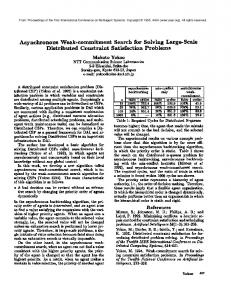
2.4 3D Machine Operation There are three types of machine cycles in a 3D state machine:

Type I. an input burst followed by a concurrent output and state burst; Type II. an input burst followed by an output burst followed by a state burst; Type III. an input burst followed by a state burst followed by an output burst. The selection of a machine cycle depends on the required level of concurrency and the combinational synthesis method used. Normally, the user of the 3D synthesis tool selects Type I or II. Type III is used only to avoid a dynamic hazard that arises in two-level AND-OR due to undirected don't cares, which will be discussed in detail in chapter 3. At power-up or after completion of the previous machine cycle, the machine waits for an input burst to arrive. In a Type I machine cycle when the machine detects that all of the terminating edges of the input burst have appeared, it generates a concurrent output/state burst (which may be empty), completing a 2-phase machine


Type I i1+ i2* o+ s-

i1- i2+

o-

Φ1

Φ2

i1- i2+

o-

Φ1

Φ2

c i1 i2 o s Φ1

Φ2 Type III

i1+ i2* s- o+ c i1 i2 o s Φ1

Φ2 Φ3

Figure 2.10: 3D machine cycles (Types I and III).

30


31

cycle. In a Type II machine cycle, when the machine detects that all of the terminating edges of the input burst have occurred, it generates an output burst (which may be empty). A state burst (which may also be empty) immediately follows the output burst, completing the 3-phase cycle. Note that an output burst enables a state burst in the \burst-mode fashion" | the state variable changes are enabled only after all the changes of the output burst have fed back. In a Type III machine cycle, a state burst is enabled by the input burst and an output burst is enabled by the state burst. Note that the state assignment used in the simple example in the last section forced the machine cycle in S to be of Type I; however, a state assignment scheme that generates a dierent type of machine cycle can be used just as well. Figure 2.10 illustrates examples of two machine cycles (Type I and Type III). The rst machine cycle begins with input burst (phase 1) hc i i i . The conditional signal c stabilizes to 1 before i res. The directed don't care signal i may remain at 0 or change to 1. In the Type I machine cycle, this input burst enables a concurrent output/state burst (phase 2), o s,. In the Type III machine cycle, this input burst enables the state burst (phase 2), s,, which, in turn, enables the output burst (phase 3), o . In the second machine cycle, an input burst, i ,i , enables an output burst, o,, and no state burst is required. Thus both the Type I and III machine cycles are identical. 1

+

1

+

+

2

2

+

+

1

1

2

+

Chapter 3 Hazard Considerations 3.1 Introduction In this chapter, we pay close attention to the correctness of the implementation and the requirements for correctness. An implementation is correct if and only if the range of possible behavior in the environment of the implementation is a subset of the range of behavior allowed by the speci cation. One way to guarantee that an implementation is correct is to transform the speci cation using a procedure each step of which preserves correctness. The main problem in ensuring the correctness of asynchronous circuits is avoiding the possibility of hazards. A hazard is broadly construed as a potential for malfunction of the implementation. We review precise characterization of various kinds of hazards and describe how each is avoided. We show that the 3D machine synthesis problem reduces to one of synthesizing hazard-free combinational logic and then show how the various sources of hazards are systematically eliminated. Figure 3.1 illustrates how the 3D machine can be viewed as a combinational logic function during each burst (Type II machine cycle is used in this example). Assume that no fed-back output change arrives at the network input until all of the speci ed changes of the output burst have appeared at the network output. The same assumption applies to the fed-back state variable changes and the state burst. These conditions will be met by inserting delays in the feedback paths as necessary. The 32

CHAPTER 3. HAZARD CONSIDERATIONS

33

machine then can be viewed as a combinational logic function 1. excited by the input changes during the input bursts (phase 1); 2. excited by the fed-back output changes during the output bursts (phase 2); 3. excited by the fed-back state variable changes during the state burst (phase 3). Note that the machine is stable at the beginning of each phase. input

Φ1 Φ2 Φ3

output

C L 2-Level AND-OR

state

Figure 3.1: Combinational view of the 3D state machine. Therefore, the 3D machine synthesis procedure follows the steps outlined below: 1. specifying a hazard-free combinational logic function that can be transformed into a hazard-free logic circuit; 2. implementing a hazard-free combinational circuit from the speci ed combinational function; 3. ensuring that the sequential circuit created by connecting feedback paths are free of hazards. The rst step of the synthesis procedure is to correctly specify a combinational logic function that conforms to the speci cation. This step must ensure that the speci ed function is free of function hazards, that is, for every set of input changes


34

and feedback signal changes with all the signals not speci ed to change set to correct values, both the static and dynamic behavior of every output is exactly as speci ed. In addition, this functional synthesis step must take measures to ensure that a hazardfree circuit exists for the speci ed function. The second step of the synthesis procedure is to correctly implement a combinational logic circuit from the combinational function speci ed in the last step. That is, this step must implement a circuit free of logic hazards. The last step of the synthesis procedure is to turn this combinational circuit into a sequential circuit by connecting outputs of the network to the inputs, that is, creating feedback paths. This step must ensure that the sequential circuit created by connecting feedback paths is free of sequential hazards, that is, the circuit behaves as speci ed as a sequential machine. In the remainder of this chapter, we examine the sources of hazards (sequential hazards, function hazards, and combinational logic hazards) in detail and provide remedies for each. The synthesis procedure itself and the algorithms are presented in chapter 4.

3.2 Sequential Hazard The correct operation of the 3D machine relies on the assumption that all of the speci ed changes of the outputs of the combinational network excited by a set of changes at the network inputs are completed before the next set of changes arrives at the network inputs. A violation of this assumption may result in a sequential hazard, the hazard that exists regardless of the correctness of the underlying combinational circuit. Both the timing characteristics of the circuit itself and the environment of the circuit can cause sequential hazards.

3.2.1 Essential Hazard We examine how the internal timing of the circuits can introduce sequential hazards. It has been assumed up to now that no change at the network output is fed back to


35

the input of the combinational network until all the changes at the network outputs that are concurrently enabled have taken place. However, this assumption may be violated if feedback delays are short compared to the dierence between the maximum and minimum feedforward delays. The hazard that arises due to the race between the arrivals of input edges and one or more fed-back output edges, enabled by the same input changes, at the network input is called essential hazard. ab xy 00 01 11 10

0 a+b+ / x+ b- / x- y-

1 a- / y+

2

00 01 00 0 00 00 00 00

11 10

11 2 11 10

10 00

1

Next-state table

ta-x

a b

a+b+ x

x+

b a

ta-a’

a’ ta-a’

y tx-X

X y = a’bX

X

ta-x +tx-X

glitch due to "fast" x

Figure 3.2: Essential hazard. The possibility of an essential hazard during a 0 ! 0 transition of an output is illustrated in gure 3.2. During the input/output burst (a b ! x ), y is speci ed to remain 0. However, if x is fed back to the network input before a0 goes low, then a 0 , 1 , 0 glitch may propagate to output y. Thus, we need to make sure that the feedback delay (tx,X ) is suciently large to avoid essential hazards. Essential hazards, in general, can be avoided simply by inserting sucient delays in the feedback paths. However, the delays in the feedback paths increase the delay constraint between last output change and next compulsory input change that must + +

+

+


36

be obeyed by the environment of the circuit. Hence, it is desirable to minimize feedback delays to improve system performance. Sometimes, it is possible to nd tighter constraints, i.e., reduce feedback delays, if the details of the implementation technology are known. t in-out Tin-prod Tin-lit in out t outf-prod outf

t outf-sv Toutf-prod Toutf-lit sv

svf t svf-prod t sv-svf

t out-outf

Figure 3.3: Timing requirements for minimum feedback delay.

Sucient Conditions for Freedom from Essential Hazards in 2-Level ANDOR If 3D machines are implemented in two-level AND-OR, a set of simple one-sided timing constraints can be used to characterize the minimum required feedback delay. We show below a set of timing constraints required for Type II machine cycles. tx,y


37

denotes the minimum delay from a transition of type x to a transition of type y, while Tx,y denotes the maximum delay (see gure 3.3). 1. t , + t ,

>T

2. t , + t ,

+t

in

out

out

out

outf

,lit .

out

3. t

outf

,sv

+t , >T , .

4. t

outf

,sv

+t , +t , sv

svf

svf

outf

,prod

in

sv

outf

in

outf

svf

>T

in

,prod .

lit

prod

>T

outf

,prod .

Usually, these inequalities are satis ed without adding delays, as should be clear by comparing the lengths of the paths followed on each side of the inequalities. Note that the requirements for a Type I machine cycle are simpler, because state variable changes are concurrent with output changes: only the rst two inequalities are needed.

3.2.2 Environmental Constraints An inherent feature of the 3D implementation is that parts of the circuit may still be unstable after a change at the network output has taken place. In some sense, this feature can help improve the performance of the system by eectively making the stabilization of the circuit and the reaction of the environment concurrent, provided that the environment is slow to react to the changes in the circuit outputs. However, if the environment reacts so fast that the circuit detects the new input arrivals before the arrival of feedback variable changes, then the circuit may malfunction. Therefore, we must have the environment delay generating certain changes. This is called the fundamental-mode environmental constraint. In practice, this is usually not a problem, because of the delays in wires between the circuit and the environment and the time for the environment to react are generally longer than it takes for the circuits to stabilize. In addition, not all the input signals have to meet this constraint, because some signals are speci ed as don't cares in the extended-burst-mode. Another form of the environmental constraint required by the extended-burstmode 3D machine are the setup time and hold time requirements: all conditional signals speci ed to stabilize must stabilize for some interval before any compulsory


38

(sampling) edge appears and must remain stable until the output/state burst is completed. This requirement is similar to the setup and hold requirements on data signals with respect to clock of synchronous ip- ops.

3.2.3 Summary The following are the timing requirements imposed by the synthesis method to guarantee correctness of the implementation. 1. feedback delay requirement : feedback variable changes are not fed-back until all enabled feedback variable changes are completed; 2. fundamental-mode environmental constraint : no compulsory edges of the next input burst may arrive until the machine is stabilized; 3. setup and hold time requirements : all conditional signals speci ed to be stable must be stabilize before any compulsory (sampling) edge appears and must remain stable until the output/state burst is completed. Assuming these timing constraints are met, we need only analyze the hazards in the combinational circuit that results from cutting feedback paths.

3.3 Function Hazard A function hazard is a non-monotonic change, i.e., more than one change, of a combinational function during a multiple-input change [23, 69]. Function hazards are problematic because they are present in every gate-level implementation of the function, if inputs to functions have arbitrary delay. Consequently, function hazards must be prevented before combinational synthesis. We consider function hazards during multiple-input changes in which some inputs are non-monotonic, i.e., change more than once. We examine the implications of allowing certain input changes to be nonmonotonic, de ne what a function hazard is in this setting, and explain how function hazards are avoided in the 3D implementations.


39

3.3.1 De nitions We summarize some de nitions and concepts from [5, 4, 53, 60] that are used in the following subsections. A logic function f is a mapping from f0; 1gn to f0; 1; g. A minterm of f is an n-tuple [x ; x ; : : : ; xn] where xi , the value of the i-th input of f , is 0 or 1. The on-set of f is the set of minterms for which f is 1; the o-set of f is the set of minterms for which f is 0; the dc-set of f is the set of minterms for which f is . A cube c, written as [c ; c ; : : : ; cn], is a vector in f0; 1; gn. A minterm [x ; x ; : : : ; xn] is a cube such that for every i 2 1; : : : ; n, xi 6= . A cube [a ; a ; : : : ; an] is said to contain another cube [b ; b ; : : : ; bn] i, for all i in 1; : : : ; n, ai = bi or ai = . A cube [a ; a ; : : : ; an] is said to intersect another cube [b ; b ; : : : ; bn] i, for all i in 1; : : : ; n, ai = bi or ai = or bi = . A literal is a variable or its complement. A product term is a boolean product of literals, and a sum of products is a boolean sum of product terms. We consider only product terms satisfying the restriction that no product term can have both a variable and its complement as inputs. With this restriction, there is a one-to-one correspondence between product terms and cubes, so we use the terms cube and product term interchangeably. Thus a product term x x x is equivalent to a cube [1; ; 0; 1; ; : : :; ]. An implicant of f is a product term which contains no o-set minterms of f . A cover C of a logic function f is a set of implicants of f such that every on-set minterm of f is contained in some cube of C but no o-set minterm. A cover is isomorphic to a sum-of-products implementation of f . If A = [a ; a ; : : : ; an] and B = [b ; b ; : : : ; bn], the transition cube C = [c ; c ; : : : ; cn] is determined so that, for i = 1; : : : ; n, ci = ai = bi , if ai = bi, and ci = , if ai 6= bi . The transition cube C , denoted as [A; B ], is the smallest cube that contains both A and B . A trajectory in [A; B ] is a vector of minterms contained [A; B ], denoted as [m ; m ; : : : ; mp], such that, for every j in 1; : : : ; p , 1, the minterms mj and mj dier in just one bit position. 1

2

1

1

2

1

2

2

1

1

1

1

2

2

2

1

1

1

2

3

2

2

4

1

2

+1


40

A combinational function has a function hazard if it changes more than once during a speci ed multiple-input change. Assume, for now, that all input changes are monotonic (we will generalize it so that some input changes can be non-monotonic in the following subsection). There is a corresponding transition cube for every multipleinput change. The transition cube contains all of the minterms in every possible trajectory of the speci ed input changes. If the function changes its value more than once along a certain trajectory, then there is a function hazard. The following \classical" de nition of function hazard adapted from [4] captures this notion precisely.

De nition 3.1 A combinational function f contains a function hazard during a multiple-input change from A to B i there exists a pair of minterms X and Y in [A; B ] (A 6= X and Y 6= B ) such that 1. X 2 [A; B ] and Y 2 [X; B ] and 2. f (A) 6= f (X ) and f (Y ) 6= f (B ).

If f (A) = f (B ), it is a static function hazard, that is, a 1 , 0 , 1 or 0 , 1 , 0 function hazard. Otherwise, it is a dynamic function hazard, that is, a 1 , 0 , 1 , 0 or 0 , 1 , 0 , 1 function hazard.

3.3.2 Generalized Transition If some inputs are allowed to change non-monotonically during multiple-input changes, the classical de nition of function hazard is inadequate. We develop a notion of generalized transition to remedy this de ciency and to provide a vehicle to discuss functional synthesis in analytical terms in chapter 4. A generalized transition (T; A; B ) de nes a set of all legal trajectories in [A; B ], where A is a start cube, B is an end cube, and T is a mapping from a set of inputs to a set of input types. There are three types of inputs: rising edge, falling edge, and level signals. Edge inputs can only change monotonically; therefore, edge inputs change at most once in a legal trajectory. Level inputs must remain constant or be unde ned (don't care), which implies that each level input must hold the same value in both


41

A and B or be unde ned in both A and B . Level inputs, if they are unde ned, may change non-monotonically, A generalized transition cube [A; B ] is the smallest cube that contains the start and end cubes A and B , as de ned before. Open generalized transition cubes , [A; B ) = [A; B ] , B , (A; B ] = [A; B ] , A, and (A; B ) = [A; B ) , A respectively. Note that [A; B ) = ;, if A = B . The start subcube A0 is a maximal subcube of A such that: 1. the value of every rising edge input i in A0 is 0, if it is in A; 2. the value of every falling edge input j in A0 is 1, if it is in A. The end subcube B 0 is a maximal subcube of B such that: 1. the value of every rising edge input i in B 0 is 1, if it is in B ; 2. the value of every falling edge input j in B 0 is 0, if it is in B . Intuitively, if edge signals have weight 1 and level signals have weight 0, the trajectories from A0 to B 0 are the maximum-weight trajectories. If every don't care input is an edge signal in (T; A; B ), [A0; B 0 ] = [A; B ] and A0 and B 0 reduce to minterms.

Lemma 3.1 For every minterm X in [A; B ], all of the minterms in every legal trajectory from X to B is contained in [X; B 0 ].

Proof: We prove by contradiction. Assume that there exists a trajectory such that one of the minterms in the trajectory is outside of [X; B 0 ].

1. [X; B 0] = [X; B ] [X; B ] contains all of the minterms in every trajectory from X to B , which contradicts the assumption. 2. [X; B 0] [X; B ] Then there exists Y contained in [X; B ] , [X; B 0] such that Y can be reached from X legally. Let X = [x ; : : : ; xn ], Y = [y ; : : : ; yn], B 0 = [b0 ; : : : ; b0n], and [X; B 0] = [c ; : : : ; cn]. For every i in 1; : : : ; n, ci = or ci = b0i. Since Y is not contained in [X; B 0 ], there exists an edge signal j such that yj 6= ^ yj 6= b0j ^ cj 6= . Because cj 6= , xj = b0j , which means xj changed once. Thus there is no legal trajectory from X to Y , which contradicts the assumption. 1

1

1

1


42

During a generalized transition (T; A; B ), each output signal is assumed to change its value at most once. Furthermore, no output change is allowed in A and B . If not, a function hazard is said to be present. Below is the new de nition of function hazard adapted for generalized transitions:

De nition 3.2 A combinational function f contains a function hazard in (T; A; B ) i

1. there exists a pair of minterms X; Y in A such that f (X ) 6= f (Y ), or 2. there exists a pair of minterms X; Y in B such that f (X ) 6= f (Y ), or 3. there exists a pair X; Y in (A; B ) such that Y 2 [X; B 0 ) (or, equivalently, X 2 (A0; Y ]) and f (A) 6= f (X ) and f (Y ) 6= f (B ).

The last criterion states that there is a function hazard if there exist two minterms X and Y in a legal trajectory from A to B such that f (A) 6= f (X ) and f (Y ) 6= f (B ). A generalized transition (T; A; B ) is a static transition for f i f (A) = f (B ); it is a dynamic transition for f i f (A) 6= f (B ). No change in level inputs can enable output changes directly, that is, at least one edge input must change from 0 to 1 or from 1 to 0 in a generalized dynamic transition. Examples of generalized transitions are shown in gure 3.4. a, b, and c are rising edge signals, and s is a level signal. Figures 3.4ac show function-hazard-free static and dynamic transitions respectively. Figure 3.4b illustrates a 1-0-1 static function hazard, and gure 3.4d does a 0-1-0-1 dynamic function hazard on the trajectory, abc : 000 ! 100 ! 101 ! 111.

3.3.3 Extended-Burst-Mode Transition An extended-burst-mode transition is a generalized transition with the following requirements: 1. For every pair of minterms X and Y in A [ [A; B ), f (X ) = f (Y ).


s: a, b, c:

43

level signal rising edge signal f=0 f=1

A = A’

A

a+

A’

a+

b+

b+ s+ s−

c+

B’ B

B = B’

(a) function−hazard−free static transition

(c) function−hazard−free dynamic transition

A = A’

A

a+

a+

b+

b+ s+ s−

A’

c+

B’ B

B = B’

(b) static function hazard

(d) dynamic function hazard

Figure 3.4: Generalized transitions.


44

2. For every pair of minterms X and Y in B , f (X ) = f (Y ).

Theorem 3.1 Every extended-burst-mode transition is function-hazard-free. Consider f during an extended-burst-mode transition from A to B . Since A A [ [A; B ), for every pair of minterms X and Y in A, f (X ) = f (Y ) by requirement 1 of the de nition of extended-burst-mode transition. This contradicts criterion 1 of De nition 3.2. For every pair of minterms X and Y in B , f (X ) = f (Y ) by requirement 2, which contradicts criterion 2 of De nition 3.2. Finally, for all X in (A; B ), f (X ) = f (A) by requirement 1, which contradicts criterion 3 of De nition 3.2. Therefore, f is free of function hazards. An edge signal that changes from 0 or to 1 or from 1 or to 0 during an extended-burst-mode transition from A to B is a terminating signal in (T; A; B ). An edge signal whose value is in B is a directed don't care in (T; A; B ). A level signal whose value is in (T; A; B ) is an undirected don't care. In a dynamic extended-burstmode transition, the output is enabled to change only after all of the terminating edges appear. Another way of describing terminating signals and don't cares is as follows: Let minterms X = [: : : ; xs; : : :] and X 0 = [: : : ; xs; : : :], where xs and xs are the values of s in X and X 0. s is a terminating signal i X 2 B implies X 0 62 B . s is a don't care (directed or undirected) i X 2 B , X 0 2 B or, equivalently, X 2 [A; B ) , X 0 2 [A; B ). A 3D machine cycle that requires no conditional signals to stabilize has transitions corresponding to an input burst and a concurrent output/state burst, if it is of Type I, or an input burst, an output burst and a state burst, if it is of Type II or III. A 3D machine cycle that requires conditional signals to stabilize has an additional transition for setting up conditional signals. Each of these transitions by itself is free of function hazards, since these are all extended-burst-mode transitions. However, as we have seen in the simple example in section 2.3.1, a function-hazard-free next-state assignment requirement for one transition may con ict with another transition. The 3D state assignment algorithm avoids this type of con ict by adding state variables when necessary, as described in the next chapter. Proof:


45

X Input Bit Vector

Output Bit Vector Y

Z State Var Bit Vector

a

b

c Layer 00 (C) e Layer 01 (E) d Layer 11 (D) f Layer 10 (F) State

a b c e, f d

Next-state

a beginning of input burst c end of input burst / beginning of output burst d end of output burst / beginning of state burst (critical race if d is not next-state) transient states d end of state burst

Figure 3.5: Critical race.


46

3.3.4 Critical Race If a transition between layers requires multiple state bit changes (see gure 3.5), the machine traverses intermediate layers (E or F ) before it settles down to the nal stable state (d). In traditional asynchronous state machines [30, 69], a critical race is said to be present if the nal stable state depends on the order in which the state bits change. In 3D machines, a critical race is said to be present if the transient states during a layer transition have dierent next values of outputs and state variables from those of the start-state of the transition. Hence, in 3D machines, a critical race is simply a manifestation of a function hazard during a state burst. We insure that the machine is free of critical races by encoding layers so that the next states of the transient states during layer transitions are the same as those of the start-state of the transition.

3.4 Combinational Logic Hazards Hazards in combinational circuits can also be introduced by the delay variations of physical gates and wires, even if the logic functions are completely and correctly speci ed, i.e., function-hazard-free. In this section, we present two dierent methods to implement hazard-free combinational logic: the two-level AND-OR implementation [53] and the multiplexor tree implementation derived from a Binary Decision Diagram (BDD) representation of the next-state function [35]. Inverter δ