Computer Systems Laboratory, Stanford University, Stanford, CA 94305 z Department of EECS, ... signals are sampled, it eliminates the need for state variable changes preceding ... This paper describes a new synthesis algorithm for asynchronous controllers ..... Figure 4: (a) BDD (b) MUX network derived from BDD (c) Sim-.
Performance-driven Synthesis of Asynchronous Controllers Kenneth Y. Yun�
Bill Liny
David L. Dill��
Srinivas Devadasz
� Department of ECE, University of California, San Diego, CA 92093 y IMEC, Kapeldreef 75, B-3001 Leuven, Belgium �� Computer Systems Laboratory, Stanford University, Stanford, CA 94305 z Department of EECS, MIT, Cambridge, MA 02139
Abstract
2 Controller Specification and Implementation
We examine the implications of a new hazard-free combinational logic synthesis method [8], which generates multiplexor trees from binary decision diagrams (BDDs) — representations of logic functions factored recursively with respect to input variables — on extended burst-mode asynchronous synthesis. First, the use of the BDD-based synthesis reduces the constraints on state minimization and assignment, which reduces the number of additional state variables required in many cases. Second, in cases where conditional signals are sampled, it eliminates the need for state variable changes preceding output changes, which reduces overall input to output latency. Third, selection variables can easily be ordered to minimize the latency on a user-specified path, which is important for optimizing the performance of systems that use asynchronous components. We present extensive evaluations showing that, with only minimal optimization, the BDD-based synthesis gives comparable results in area with our previous exact two-level synthesis method. We also give a detailed example of the specified path optimization.
In this section, we summarize a design style, called extended burstmode, and an implementation style, called 3D, to specify and implement asynchronous controllers for heterogeneous systems — systems with both synchronous and asynchronous components. These topics have been discussed in more detail in previous publications [23, 22].
6
ok− frin− / faout−
0
ok* frin+ dackn+ / faout+ 5
frin* dackn− / dreq−
ok+ frin* / dreq+ 1
2
frin+ dackn+ / faout+
1 Introduction There have been many recent advances in asynchronous circuits and systems, both in tool design [1, 2, 3, 5, 7, 9, 10, 12, 13, 16, 15, 20, 21, 22] and actual systems design [6, 9, 10, 11, 14, 17]. However, for maximum acceptability, it is imperative to be able to synthesize circuits that work with existing systems, which are largely made out of synchronous components. One particularly promising design style is the extended-burst-mode [23]. This paper describes a new synthesis algorithm for asynchronous controllers specified in extended-burst-mode [23]. This algorithm assumes the target implementation to be a combinational circuit with both primary outputs and state variables fed back. The combinational circuit is derived from a Binary Decision Diagram [4] using a recently developed hazard-free combinational synthesis method [8]. This algorithm is designed, first and foremost, to minimize output latency. This new approach has many advantages over other synthesis methods [15, 16, 23, 22], which implement the combinational logic as two-level AND-OR circuits. In many cases, the circuits synthesized using this new method have considerably lower output latencies than the circuits synthesized by the method in [23]. Furthermore, this method provides a platform to further minimize the delay on user-specified input/output path, which can be very important for achieving high performance in systems that use asynchronous components. � Supported by the Semiconductor Research Corporation, Contract no. 93-DJ-205. y Supported by the EXACT project under the program ESPRIT 6143 of the European Commission z Supported by the NSF Young Investigator Award
Permission to copy without fee all or part of this material is granted, provided that the copies are not made or distributed for direct commercial advantage, the ACM copyright notice and the title of the publication and its date appear, and notice is given that copying is by permission of the Association for Computing Machinery. To copy otherwise, or to republish, requires a fee and/or specific permission.
frin* dackn− / dreq−
3
frin− / dreq+ faout− frin* dackn− / dreq−
4
frin* dackn− / dreq−
Figure 1: Extended-burst-mode Specification. Figure 1 shows an example of an extended burst-mode specification. Signals not enclosed in angle brackets and ending with + or are terminating signals. These are edge signals. The signals enclosed in angle brackets are conditionals, which are level signals whose values are sampled when all of the terminating edges associated with them have occurred. A conditional a+ can be read “if a is high” and a can be read “if a is low.” A state transition occurs only if all of the conditions are met and all the terminating edges have appeared. A signal ending with an asterisk is a directed don’t care. If a is a directed don’t care, there must be a sequence of state transitions in the machine labeled with a� . If a state transition is labeled with a� , the following state transitions in the machine must be labeled with a� or with a+ or a (the terminating edge for the directed don’t care). This specification describes a state machine having a conditional input (cntgt1), 3 edge inputs (ok; frin; dackn), and 2 outputs (dreq; faout). Consider the state transitions out of state 4. The behavior of the machine at this point is: “if cntgt1 is low when dackn falls, change the current state from 4 to 5 and lower the output dreq; if cntgt1 is high when dackn falls, change the current state from 4 to 2 and
h i
h i
1994 ACM 0-89791-690-5/94/0011/0550 $3.50
lower output dreq.” A directed don’t care may change at most once during a sequence of state transitions it labels, i.e., directed don’t cares are monotonic signals, and, if doesn’t change during this sequence, it must change during the state transition its terminating edge labels. A terminating edge which is not immediately preceded by a directed don’t care is called compulsory, since it must appear during the state transition it labels. frin is low when the specification is in state 4. It can rise at any point as the machine moves through states 5 and 6 or through state 2, depending on the level of cntgt1, and it must have risen by the time the machine moves to states 6 or 2, because the terminating + edge frin appears between states 5 and 6 and between 4 and 2. The input signals are globally partitioned into level signals (conditionals), which can never be used as edge signals, and edge signals (terminating or directed don’t care), which can never be used as level signals. If a level signal is not mentioned on a particular state transition, it may change freely. If an edge signal is not mentioned, it is not allowed to change. More generally, an extended-burst-mode asynchronous finite state machine [23] is specified by a state diagram which consists of a finite number of states, a set of labeled state transitions connecting pairs of states, and a start state. Each state transition is labeled with a set of conditional signal levels and two sets of signal edges: an input burst and an output burst. An output burst is a set of output edges, and an input burst is a non-empty set of input edges (terminating or directed don’t care), at least one of which must be compulsory. In a given state, when all the specified conditional signals have correct values and when all the specified terminating edges in the input burst have appeared, the machine generates the corresponding output burst and moves to a new state. Specified edges in the input burst may appear in arbitrary temporal order. However, the conditional signals must stabilize to correct levels before any compulsory edge in the input burst appears and must hold their values until after all of the terminating edges appear. The minimum delay from the conditional stabilizing to the first compulsory edge is called the setup time. Similarly, the minimum delay from the last terminating edge to the conditional changing is called the hold time. Actual values of setup and hold time of conditional signals with respect to “sampling” edges depend on the implementation. Conditional signal levels need not be stable outside of the specified sampling periods. Each signal specified as a directed don’t care may change its value monotonically at any time including during output bursts, unless it is already at the level specified by the next terminating edge. Outputs may be generated in any order, but the next set of compulsory edges from the next input burst may not appear until the machine has stabilized. This requirement — the environment must wait generating the next set of compulsory edges until the circuit stabilizes — called the fundamental-mode environmental constraint. There is an additional restriction to extended-burst-mode specifications, called the distinguishability constraint, which prevents ambiguity among multiple input bursts emanating from a single state: For every pair of input bursts i and j from the same state, either the conditions are mutually exclusive, or the set of compulsory edges in i is not a subset of the set of all possible edges in j . 2.1 3D Implementation A 3D asynchronous finite state machine is a 4-tuple (X; Y; Z; � ) where X is a non-empty set of primary input symbols, Y a nonempty set of primary output symbols, Z a possibly empty set of Z Y Z internal state variable symbols, and � : X Y is a next-state function. The hardware implementation of a 3D state machine (see figure 2) is a combinational network, which implements the next-state function, with the outputs of the network fed back as inputs to the network. There are no explicit storage
� � ! �
input
output Hazard−free Combinational Network
state
Figure 2: 3D Asynchronous State Machine.
elements such as latches, flip-flops or C-elements in a 3D machine. A 3D implementation of an extended-burst-mode specification is obtained from the next-state table, a 3-dimensional tabular representation of � . The next state of every reachable state must be specified in the next-state table; the remaining entries are don’t cares. A machine cycle consists of an input burst followed by a concurrent output and state burst. Initially or after completion of the previous output and state burst, the machine waits for an input burst to arrive. When the machine detects that all of the terminating edges of the input burst have appeared, it generates a concurrent output/state burst, which may be empty. 2.2
2-level Synthesis
In the 3D implementation of extended-burst-mode machines, no fed-back output or state variable change arrives at the network input until all of the specified edges in the output and state burst have appeared at the network output. These conditions are met by inserting delays in the feedback paths as necessary. A 3D machine can then be viewed as a combinational network alternately excited by a set of input edges (during an input burst) and by a set of fed-back output and state variable edges (during an output/state burst). Thus each burst is a generalized transition of inputs to the combinational network, as described below: Generalized transition
A generalized transition is a triple (T; A; B ) where T is a mapping from a set of inputs to a set of input types, A a start-cube, and B an end-cube. There are three types of inputs: rising edge, falling edge, and level signals. Edge inputs can only change monotonically. Level inputs must remain constant or undefined (don’t care), which implies that each level input must hold the same value in both A and B or be undefined in both A and B . Level inputs, if they are undefined, may change non-monotonically, A generalized transition cube [A; B ] is the smallest cube that contains the start- and end-cubes A and B . It represents the set of all minterms that can be reached during a legal transition from a point in start-cube A to a point in end-cube B , assuming that the inputs can change in arbitrary order. Open generalized transition cubes, [A; B ), (A; B ], and (A; B ), denote [A; B ] B , [A; B ] A, and [A; B ) A respectively. Note that [A; B ) = , if A = B . The start-subcube A0 is a maximal subcube of A such that the value of every rising edge input i in A0 is 0, if it is in A, and the value of every falling edge input j in A0 is 1, if it is in A. The end-subcube B 0 is a maximal 0subcube of B such that the value of every rising edge input i in B is 1, if it is in B , and the value of every falling edge input j in B 0 is 0, if it is in B . Intuitively, the longest transitions, disregarding non-monotonic signals, are those that lead from A0 to B 0 .
;
� �
�
�
�
is in [A; B ] is an undirected don’t care. In a dynamic extendedburst-mode transition, the output is enabled to change only after all of the terminating edges appear. In order for a 2-level AND-OR implementation of an output or a state variable function to be hazard-free, a set of covering requirements [23, 16] must be satisfied for each burst, i.e., extended-burstmode transition. It was shown in [23] that it is not always possible to satisfy the covering requirements for all of the specified bursts under the presence of non-monotonically changing (undefined) conditionals, if the single transition time (STT) state assignment [19] is used. The approach taken in [23] was to insert a state burst between a conditional input burst and the corresponding output burst in order to guarantee that the covering requirements can be satisfied for all of the specified bursts. Unfortunately, the early state burst between the input burst and output burst increased the input/output latency significantly, and also tended to increase the circuit area.
level signal rising edge signal
s: a, b, c:
f=0 f=1 A = A’
A
a+
A’
a+
b+
c+
b+ s+ s−
B’ B
B = B’
(a) function−hazard−free static transition
(c) function−hazard−free dynamic transition
A = A’
3 BDD-based Combinational Synthesis
A
a+
A’
b+
a+ c+
b+ s+ s−
B’ B
B = B’
(b) static function hazard
(d) dynamic function hazard
Figure 3: Generalized Transition Cube [A; B ]. A generalized transition (T; A; B ) is a static transition for f iff f (A) = f (B ); it is a dynamic transition for f iff f (A) 6= f (B ).
No change in level inputs can enable output changes directly, that is, at least one edge input must change from 0 to 1 or from 1 to 0 in a generalized dynamic transition. During a generalized transition (T; A; B ), each output signal is assumed to change its value at most once. If not, a function hazard is said to be present. Below is the definition of function hazard adapted for generalized transitions: Definition 1 A combinational function f contains a function hazard during a generalized transition (T; A; B ) iff
6
1. there exists a pair of minterms X; Y in A such that f (X ) = f (Y ), or
6
2. there exists a pair of minterms X; Y in B such that f (X ) = f (Y ), or 3. there exists a pair X; Y in (A; B ) such that Y f (A) = f (X ) and f (Y ) = f (B ).
6
6
2 [X; B 0 ) and
An extended-burst-mode transition is a generalized transition with the following requirements: 1. For every pair of minterms X and Y in [A; B ), f (X ) = f (Y ).
2. For every pair of minterms X and Y in B , f (X ) = f (Y ).
Theorem 1 Every extended-burst-mode transition is functionhazard-free.
�
�
An edge signal that changes from 0 or to 1 or from 1 or to 0 during an extended-burst-mode transition from A to B is a terminating signal in [A; B ]. An edge signal whose value is in B is a directed don’t care in [A; B ]. A level signal whose value
�
In this paper, we use a new BDD based combinational synthesis technique from [8]. This approach imposes a different set of requirements to guarantee freedom from all hazards, but we will show that it is always possible to meet these requirements without the multiple transition time state assignment that was required in the method of [23], resulting in greatly reduced latency in many cases. Combinational networks that describe next-state functions are constructed from a BDD (binary decision diagram) description. The basic gates that comprise combinational networks are ANDs, ORs, NANDs, NORs, inverters, and MUXes. We assume that every basic gate is atomic, i.e., a single transition of a gate input cannot cause a multiple transitions at the output. We do not rely on inertial delays, that is, we assume a pure gate delay model, and allow for arbitrary wire delays. 3.1
Multiplexer Networks derived from BDDs
The following definition of a Binary Decision Diagram is from [4]. Definition 2 A Binary Decision Diagram is a rooted, directed graph with vertex set V containing two types of vertices. A nonterminal vertex v has as attributes an argument index index(v ) 1; : : : ; n and two children low (v ); high(v ) V . A terminal 0; 1 . vertex v has as attributes a value value(v )
f
g
2
2
2f g
The correspondence between a BDD and a Boolean function is defined as below: Definition 3 A Binary Decision Diagram G having root vertex v denotes a function fv defined recursively as: 1. If v is a terminal vertex: (a) If value(v ) = 1, then fv = 1. (b) If value(v ) = 0, then fv = 0. 2. If v is a non-terminal vertex with index(v ) = i, then
fv (x1 ; : : : ; xn ) = xi � flow (v ) (x1 ; : : : ; xn ) + xi � fhigh(v ) (x1 ; : : : ; xn ). xi is called the decision variable for vertex v.
In addition, 1. Each decision variable occurs at most once on every path from a terminal vertex to the root vertex,
6
2. A reduced BDD is a BDD in which low(v ) = high(v ) for any vertex v and no two subgraphs are identical.
A reduced ordered BDD (ROBDD) is a canonical form with the following restriction: for any non-terminal vertex v , if low(v ) is a non-terminal, then index(v ) < index(low(v )), and if high(v ) is a non-terminal, then index(v ) < index(high(v )). A reduced free BDD (free BDD) is a BDD which does not require a strict variable ordering (unlike in an OBDD) but still requires that each decision variable is encountered at most once when traversing a path from a terminal vertex to the root vertex. f
f a
a 0
1
0
0
b 1
q
1
0
1
1
0
a
1
1
0
0
q
b 0
1
b
c
0
f 0
1
c
1
1 0
1
0
1
0
1
1
0
b
q c b
0 (a)
(b)
(c)
Figure 4: (a) BDD (b) MUX network derived from BDD (c) Simplified network (by constant propagation). A multi-level network can be derived directly from a BDD by replacing each vertex with a two-input MUX with the decision variables as the select inputs of the MUXes. Figure 4b shows a MUX network derived from the BDD in figure 4a. If one or more input of a MUX is constant, the MUX can be replaced with a simpler gate, such as a NAND or a NOR. This constant propagation is carried out topologically from inputs to outputs. Figure 4c shows an equivalent network after the constant propagation. 3.2 Hazard-free Combinational Synthesis We use the approach from [8] to synthesize hazard-free combinational circuits under extended-burst-mode transitions. This method is based on building a BDD for a specified function and deriving a multi-level circuit from it. To ensure that the resulting multi-level circuit is hazard-free, a requirement called the trigger signal ordering (TSO) must be satisfied. This requirement imposes constraints on the variable ordering of the BDD. It was shown in [8] that if this variable ordering is satisfied, then the resulting multi-level circuit is free of logic hazards for a set of specified transitions. Note that every input change in [8] was assumed to be monotonic during each transition. We will prove that the resulting circuit is free of logic hazards for a set of specified extended-burst-mode transitions, in which some inputs may change non-monotonically, as long as the TSO requirement is satisfied. A trigger state is a state in which an input change enables the output to change. A trigger signal is an input signal whose transition enables the output to change; a non-trigger signal is an input signal which is enabled to change but cannot by itself enable the output to change. The TSO requirement states that trigger signals in a trigger state must appear before the non-trigger signals of the same trigger state in the variable ordering. In the generalized transition cube that corresponds to an extended-burst-mode dynamic transition, all terminating signals are trigger signals in one or more minterms, because terminating edges can appear in any temporal order and the last one that appears is a trigger signal. Note that no terminating signal can be a non-trigger signal, because no output change can be enabled until all terminating edges appear. Furthermore, all don’t care signals (directed
or undirected) are non-trigger signals in one or more minterms, because their values may change anywhere, including in the trigger states, in the generalized transition cube. Clearly, no don’t care signal can be a trigger signal in any minterm in the generalized transition cube, because don’t care signals can never enable outputs to change. Therefore, we can impose a set of ordering requirements, which do not conflict, as a sufficient condition for hazard freedom per generalized transition cube, although the TSO requirement in [8] is an imposition on each trigger state in the transition cube. Now we can state the variable ordering requirements for the extended-burst-mode transitions as follows: Along every path from root to terminal of the BDD whose corresponding cube intersects the generalized transition cube, no don’t care signal of a dynamic transition appears before a terminating signal of the same. Here, we prove that the combinational network derived from a reduced free BDD description is hazard-free during an extendedburst-mode transition as long as the BDD satisfies the variable ordering requirement for the transition stated above. Lemma 1 If (T; A; B ) is an extended-burst-mode transition for f , then fs (X ) = fs (X ) for every don’t care signal s in (T; A; B ) and for every minterm X in [A; B ]. Definition 4 Subtransitions: 1. If s is not a constant 0 in (T; A; B ), (T; As ; Bs ) is a subtransition of (T; A; B ) with the value of s fixed to 1. 2. If s is not a constant 1 in (T; A; B ), (T; As ; Bs ) is a subtransition of (T; A; B ) with the value of s fixed to 0. Note that (T; As ; Bs ) = (T; A; B ), if s is a constant 1 in (T; A; B ), and (T; As ; Bs ) = (T; A; B ), if s is a constant 0 in (T; A; B ). Lemma 2 If (T; A; B ) is an extended-burst-mode transition for f , then 1. (T; As ; Bs ) is an extended-burst-mode transition for fs , if s is not a constant 0; 2. (T; As ; Bs ) is an extended-burst-mode transition for fs , if s is not a constant 1. Corollary 1 If (T; A; B ) is an extended-burst-mode dynamic transition for f and s is a don’t care in (T; A; B ), then (T; As ; Bs ) is an extended-burst-mode dynamic transition for fs and (T; As ; Bs ) for fs . Corollary 2 Static transitions of cofactors: 1. (T; As ; Bs ) is a static transition for fs if (T; A; B ) is an extended-burst-mode transition for f and s is a falling terminating signal. 2. (T; As ; Bs ) is a static transition for fs if (T; A; B ) is an extended-burst-mode transition for f and s is a rising terminating signal. Theorem 2 The combinational network C derived from a reduced BDD (ordered or free) description of f is hazard-free during an extended-burst-mode transition if it satisfies the variable ordering requirement for the transition: no don’t care signal appears before a terminating signal.
Proof: We prove by induction on the number of variables. Base case: The sole input of the network is connected to the select input of the multiplexor. The other input terminals are connected to a constant 1 or 0. Since the multiplexor is atomic and only the select input can change, f is hazard-free. Inductive hypothesis: Now assume that a combinational network derived from a reduced BDD representation of an n-input 1), which satisfies the variable ordering requirefunction (n ments for an extended-burst-mode transition, is hazard-free during the extended-burst-mode transition. Now consider the network C derived from a reduced BDD representation of function f with n + 1 input variables and an extended-burst-mode transition (T; A; B ) for f . Assume that the select input of the multiplexor driving the output of C is s and the data inputs are fs and fs , the Shannon cofactors of f with respect to s and s. Then (T; As ; Bs ) is an extended-burst-mode transition for fs if s is not a constant 0, and (T; As ; Bs ) is for fs if s is not a constant 1, by Lemma 2. Since f satisfies the variable ordering requirements, so do fs and fs . Therefore, fs is hazard-free if s is not a constant 0, and fs is hazard-free if s is not a constant 1, by the inductive hypothesis. We will consider 3 cases: s is a constant, s is a don’t care, and s is a terminating signal.
�
1.
2.
s is a constant: The multiplexor is a wire as long as s remains constant. Thus, if s = 0, f = fs is hazard-free since s is not a constant 1. Likewise, f is hazard-free, if s = 1. s is a don’t care: First we prove by contradiction that (T; A; B ) must be a static transition for f if s is a don’t care. Assume that (T; A; B ) is a dynamic transition for f . By Corollary 1, (T; As ; Bs ) is an extended-burst-mode dynamic transition for fs . Suppose s remains at 1 while fs changes. Then the change in fs propagates to f , which means that there is a terminating signal that enables f to change, regardless of s, violating the variable ordering requirement.
By Lemma 1, f (X ) = fs (X ) = fs (X ) for every X in A; B ]. Therefore, (T; As ; Bs ) and (T; As ; Bs ) are static 0 or both 1 1, transitions of same type, that is, both 0 for fs and fs respectively. By the inductive hypothesis, fs and fs are hazard-free, therefore constant. Since the multiplexor is atomic, f is hazard-free. [
3.
!
!
s is a terminating signal: Without loss of generality, consider only the case in which s rises. By Corollary 2, fs undergoes a static transition. By the inductive hypothesis, both fs and fs are hazard-free. Consider the case in which fs = 0. We prove by contradiction that fs must rise or remain a constant. Assume that fs is initially 1 and falls to 0, but s rises first. Since fs = 0 and fs = 1 initially, f is enabled to rise as s rises. This is a static function hazard, since f is assumed to be 0 at the end of the transition. Thus fs must rise or remain a constant; in both cases, f is hazard-free. Similarly, we can prove that f is hazard-free when fs = 1, by proving that fs must fall or remain a constant. 2
Lemma 3 There always exists a BDD that satisfies the variable ordering requirements for two dynamic input burst transitions from a specification state. Proof: For every pair of state transitions (u; v ) and (u; w) emanating from state u, there exist a compulsory transition signal i in the input burst of (u; v ) and j in the input burst of (u; w) such that i is a constant in the input burst of (u; w) and j is a constant in the input burst of (u; v ). If i and j appear before any other variable
involved in the ordering, all variable ordering requirements can be satisfied in the sub-BDDs. 2 Our strategy is to build an ROBDD using a global variable ordering, if such an ordering can be found, or to build a free BDD. If no global order exists, there is always a variable that can appear first. This variable partitions the function into a left and right BDD. The left and right BDDs do not have to have the same variable order, so they can be constructed recursively using the same method. In this 3D implementation of extended-burst-mode machines, only input bursts can be dynamic transitions. If a unique code is assigned to each specification state, we can always use fedback state variables as partitioning variables, so that the variable ordering requirements of each specification state are satisfied locally in each partition. Therefore, there exists a hazard-free free BDD implementation for every legal extended-burst-mode specification. State minimization is also constrained to avoid creating variable ordering conflicts.
4 Sequential Synthesis Procedure The sequential synthesis procedure consists of the following three steps: (1) hazard-free state assignment (2) hazard-free state minimization (3) state encoding. 4.1
Hazard-free State Assignment
We describe an algorithm for simultaneously minimizing and assigning states which always results in a hazard-free singletransition-time (STT) state assignment. In contrast, the previous algorithm for extended-burst-mode [23] use a multiple-transitiontime assignment: a state variable change was required before an output change, increasing latency significantly. Indeed, it can be shown that multiple transitions are necessary for extended-burstmode when implemented with 2-level AND-OR logic, so the use of BDDs has an inherent performance benefit. This algorithm builds a primitive next-state table — a 3dimensional table with X -axis representing the input bit vector, Y -axis the output bit vector, and Z -axis the specification states. The algorithm assigns, according to the extended-burst-mode semantics, a next state, which consists of two components: next outputs and next specification state, to entries in the table. An XY plane of the primitive next-state table is called a layer. Initially, each specification state is assigned to a unique layer. The algorithm then collapses the primitive next-state table into a reduced next-state table by merging compatible specification states without violating TSO requirements. In order to describe the primitive next-state table construction formally, a formal definition of the extended-burst-mode specification, adapted from the definition of the burst-mode specification in [16], is needed. An extended-burst-mode specification is a directed graph, G = (V; E; C; I; O; v0 ; cond; in; out), where V is a finite set of states; E V V is the set of state transitions; C = c1 ; : : : ; cl is the set of conditional inputs; I = x1 ; : : : ; xm is the set of edge inputs; O = z1 ; : : : ; zn is the set of outputs; v0 V is the unique start state; cond labels each state transition with a set of conditional inputs; in and out are labeling functions used to define the unique entry cube of each state. The function cond : E 0; 1; l defines the values of 0; 1; m defines the conditional inputs. The function in : V 0; 1 n the values of the edge inputs and the function out : V defines the values of the outputs upon entry to each state. Labeling functions transIN and transOUT are derived from (I ) defines the set of edge input graph G. transIN : E (O ) defines the changes (input burst) and transOUT : E set of output changes (output burst). ( (I ) and (O) denote the power set of inputs and the power set of outputs respectively.)
f
f g
g
�
�
f
2
!f
�g
!P
P
!f
!P
�g !f g
P
g
2
Given a state transition, (u; v ) E , xi + is in the input burst iff ini (v ) = 1 ini (u) = 1, xi is in the input burst iff ini (v ) = 0 ini (u) = 0, and xi � is in the input burst iff ini (v ) = . That is, xi transIN (u; v) iff ini (u) = ini (v) ini (v) = . Similarly, zj + is in the output burst iff outj (v) = 1 outj (u) = 0, zj is outj (u) = 1. That is, zj in the output burst iff outj (v ) = 0 transIN (u; v ) iff outj (u) = outj (v ). Let ctransIN (u; v ) = xi transIN (u; v) ini (u) = ini (v ) = . The unique entry condition is satisfied by the above definition. The remaining requirements to ensure well-formed specifications are:
^ 2
6
^
6
6
f 2 � �
6
j
_ ^
^ 6 �^
�
�
2
6 �g
Every input burst must contain a compulsory edge. That is, for every state transition (u; v ), there exists xi transIN (u; v ) such that ini (u) = ini (v ) = .
6 �^
2
6 �
Every pair of transitions emanating from the same state must satisfy the distinguishability constraint. That is, for every pair, (u; v ); (u; w ) E , ctransIN (u; v) transIN (u; w) implies that either v = w or cond(u; v ) and cond(u; w) are mutually exclusive, that is, there exists k such that condk (u; v ) = condk (u; w) condk (u; v ) = condk (u; w) = .
2
�
6 6 � � For every sequence of state transitions, u ! v1 ! � � � ! vn ! w, with n � 1 and ini (u) = ini (w) 6= �, there exists k 2 1; : : : ; n such that ini (vk ) = 6 �. ^
6 �^
Given an extended-burst-mode specification, G, as described above, let W be the set of conditional input bit vectors (c1 ; : : : ; cl ) ci 0; 1 ; i 1; : : : ; l , X be the set of edge 0; 1 ; j 1; : : : ; m , input bit vectors (x1 ; : : : ; xm ) xj yk and Y be the set of output bit vectors (y1 ; : : : ; yn ) 0; 1 ; k 1; : : : ; n . A primitive next-state table is defined as T = (V; W; X; Y; �; �), where V is the set of specification states, V and � : V W X Y and � : V W X Y 0; 1; n define the next specification state function and the next output function respectively. Below, we describe the next-state assignment. L(u) is a symbolic code assigned to state u. [cond(u; v ); in(v ); out(u); L(u)] denotes a cube in 0; 1; l+m+n+r , where r is the length of state variable bit vectors. Of course, the actual value of r will not be determined until the state encoding is done. in the place of conditional inputs is a shorthand notation, meaning that all conditional inputs are . in0 is defined as: for all j 1; : : : ; m,
f
j
2f g 2 g f j 2f g 2 g f j 2 g f g 2 � � � ! [f�g � � � ! f �g f
�g
�
�
in0 j (u) =
n
2
inj (u) if 9(u; v ) : inj (v ) 6= �
�
otherwise
The next-state assignment is as follows: For all and for every state transition, (u; v )
�
�
�
:
k 2 1; : : : ; n
Conditional input burst setup: for all M in [A; B ], �k (M ) = outk (u) and � (M ) = where A = [ ; in(0 u); out(u); L(u)], B = [ ; in (u); out(u); L(u)].
u,
Input burst: for all M in [A; B ), where
u,
� �
�k (M ) = outk (u) and �(M ) A = [cond(u; v); in(u); out(u); L(u)], B = [cond(u; v); in(v); out(u); L(u)].
=
Output/state burst: for all M in [A; B ], �k (M ) = outk (v ) and � (M ) = v , where A = [cond(u; v); in(v); out(u); L(u)], B = [cond(u; v); in(v); out(v); L(v)].
4.2
Hazard-free State Minimization
In the next step, the algorithm transforms the primitive next-state table into a reduced next-state table by merging layers. Specification states can be merged into a common layer, iff they are compatible, as described below. Definition 5 States u and u v) iff for every s in W
�
1. 2. 3.
v
in
V
are compatible (denoted as
�X �Y, �(u; s) = � _ �(v; s) = � _ �(u; s) = �(v; s) and �(u; s) = � _ �(v; s) = � _ �(u; s) � �(v; s) and if outk (u) = outk (v ) for all k 2 1; : : : ; n, then for every pair
of state transitions, (u; wu ) and (v; wv ), i is a terminating signal in (u; wu ) and j is a don’t care in (u; wu ) imply that i is a terminating signal in (v; wv ) or j is a don’t care in (v; wv ), ini (wu ) = inj (wu ) = that is, ini (wu ) = ini (u) implies ini (wv ) = ini (v ) ini (wv ) = or inj (wv ) = .
6
6
^ ^
6 �^ 6 �
�
�
Informally, the third criterion states that no input burst from u has conflicting ordering requirements with an input burst in v that has identical values of fed-back outputs. The state minimization and encoding to complete the sequential synthesis are described in [22].
5 Path Optimization Example In synchronous designs, one of the important design objectives is to carefully balance the computation blocks so that no part of the circuits are idle while other parts are busy because the clock period is determined by the worst-case delay of all the computation blocks. However, asynchronous designs can proceed immediately upon receipt of a completion signal, so it is often desirable to create highly unbalanced asynchronous circuits, where one path has been optimized, possibly at the expense of others, to optimize overall system performance. To illustrate this point and also provide a nice circuit example, we consider a hypothetical problem posed by Ivan Sutherland [18]. When the circuit in figure 5 detects a transition on r (request), if sel is high, it signals on s2 to start an expensive operation “C”, then signals completion on a when it receives r2 from the operation; otherwise, it does nothing except signal a as quickly as possible. It is quite likely in this situation that the designer would want the minimum possible latency from r to a in this case to maximize overall system performance. The implementation shown does not do a very good job of minimizing this latency, because there would be a significant delay from r to s1 for most implementations along with an additional delay through the “merge” element, which is an XOR gate. This controller uses the 2-phase signaling, i.e., every transition of a signal is considered as a request or acknowledge. We have included the extended-burst-mode specification in figure 5. If sel is sampled high when r (request) toggles, the controller toggles s2 , signaling the block C to begin a computation. When C finishes the computation, it toggles r2 ; the controller then toggles a (acknowledge). However, if sel is sampled low when r toggles, then the controller toggles a directly. The result of applying our synthesis method from [23] turned out to be remarkably similar to the naive design at the top of figure 5, which we found disappointing. Our hand designs were better, but also unsatisfactory. However, using this new BDD-based approach, we were able to produce an extremely good result: the latency from r to a was just the delay from the select input to the output of a single multiplexor. The solution was generated by building a BDD so that the decision variable r is placed as close to the output a
sel
a
s1
Merge
a
r
r
s2
C
s2
0
1
1
0
0
1
y
y
0
1
r2 r2
0
1
Computation block
0 1
r+ / a+
0 r− / a−
4
r+ / s2+
0
r2− / a−
1
sel
y s2 y s2
1 Figure 6: Select/Merge Implementation.
r− / s2+
5
r2+ / a+ r− / a−
2 r+ / a+
r2+ / a−
6
synthesis system for self-timed circuits. In ICCAD-92, pp 587–591.
r− / s2−
r+ / s2−
3
r2− / a+
7 Figure 5: Select/Merge Example.
as possible, while satisfying other requirements to keep the circuit hazard-free. The final implementation is shown in figure 6. It would be very easy to generalize this idea by allowing the user to specify a set of particular paths to optimize, in order of priority. The variable ordering in the BDD could be chosen to put the high-priority inputs as close as possible to the output, subject to the correctness constraints imposed by TSO, etc.
6 Experiments We modified the 3D synthesis tool described in [23], in particular, the hazard-free state assignment and combinational synthesis steps. We used this modified tool in conjunction with the combinational synthesis tool [8] to perform experiments (see table 1) on many examples previously synthesized by the method described in [23]. With very modest efforts to find the optimal variable order (we tried a few random orderings and picked the best result), most of the examples required less area than the previous method, primarily because of the reduction in the number of state variables due to simpler state assignment. For a minority of the examples, area increased somewhat. We believe that the area results will be further improved with the development of heuristic variable ordering algorithms tuned to our application. A more important issue is output latency. Out of 39 examples synthesized, 24 of them (the names with *) previously required state variable changes before output changes for some of the specified transitions. In these cases, using BDD-based synthesis rather than 2-level synthesis improved the output latency by 100% or more.
References [1] V. Akella and G. Gopalakrishnan. SHILPA: A high-level
[2] P. Beerel and T. Meng. Automatic gate-level synthesis of speed-independent circuits. In ICCAD-92, pp 581–586. [3] E. Brunvand and R. F. Sproull. Translating concurrent programs into delay-insensitive circuits. In ICCAD-89, pp 262– 265. [4] R. E. Bryant. Graph-based algorithms for boolean function manipulation. IEEE Transactions on Computers, C35(8):677-691, August 1986. [5] T.-A. Chu. Synthesis of self-timed VLSI circuits from graphtheoretic specifications. Technical Report MIT-LCS-TR-393, MIT, 1987. Ph.D. Thesis. [6] A. Davis, W. Coates, and K. Stevens. The Post Office experience: designing a large asynchronous chip. In HICSS, Volume I, pp 409–418, January 1993. [7] L. Lavagno and A. Sangiovanni-Vincentelli. Algorithms for synthesis and testing of hazard-free asynchronous circuits. Kluwer Academic, 1993. [8] B. Lin and S. Devadas. Synthesis of Hazard-Free Multi-level Logic Implementations under Multiple-Input Changes from Binary Decision Diagrams. In This Proceedings. [9] A. J. Martin. Programming in VLSI: From communicating processes to delay-insensitive VLSI circuits. In C. A. R. Hoare, editor, UT Year of Programming Institute on Concurrent Programming, Addison-Wesley, 1990. [10] Teresa H. Meng. Synchronization Design for Digital Systems. Kluwer Academic, 1990. [11] C. E. Molnar, T.-P. Fang, and F. U. Rosenberger. Synthesis of delay-insensitive modules. In Henry Fuchs, editor, 1985 Chapel Hill Conference on Very Large Scale Integration, pp 67–86. CSP, Inc., 1985. [12] C. W. Moon, P.R. Stephan, and R.K. Brayton. Specification, synthesis, and verification of hazard-free asynchronous circuits. In ICCAD-91, pp 322–325. [13] C. Myers and T. Meng. Synthesis of timed asynchronous circuits. In ICCD-92, pp 279–284.
iccad93ex* edac93ex* condtest* dff1* dff2* sr2* sr2x2* q42 select2ph* selmerge2ph* sin ring-counter binary-counter binary-counter-co pe-send-ifc pe-rcv-ifc dramc cache-ctrl tsend* isend* trcv* ircv* tsend-bm* trcv-bm* isend-bm* ircv-bm* tsend-csm* trcv-csm* isend-csm* ircv-csm* abcs stetson-p1 stetson-p2 stetson-p3 biu-fifo2dma* fifocellctrl scsi-targ-send* scsi-init-send* scsi-init-rcv-sync
Specification States / Primary Transitions In Out 3 4 2 2 4 5 3 2 4 5 3 2 4 6 2 2 4 6 2 2 8 12 2 3 8 20 3 3 4 4 2 2 4 8 2 2 8 12 3 2 13 17 3 4 8 8 1 2 32 32 1 4 32 32 1 5 11 14 5 3 12 15 4 4 12 14 7 6 38 49 16 19 22 30 7 4 24 32 7 4 16 22 7 4 16 22 7 4 11 14 6 4 8 10 6 4 12 15 6 4 8 10 6 4 11 14 6 4 8 10 6 4 12 15 6 4 8 10 6 4 23 33 9 7 31 38 13 14 25 27 8 12 8 11 4 2 11 13 5 2 3 3 2 2 7 8 4 2 7 8 4 2 4 5 3 1
State vars added 2-level BDD 2 0 2 1 2 1 2 0 2 0 3 2 4 2 1 1 2 0 2 1 3 4 1 1 3 3 3 3 2 2 3 2 1 0 1 1 5 5 5 7 3 2 3 2 2 2 3 1 3 3 3 1 4 3 3 2 3 4 3 2 3 3 3 3 4 4 1 0 5 5 1 1 3 3 2 2 1 1
Total literals 2-level BDD 20 6 32 20 30 23 28 12 28 12 82 55 131 130 27 24 42 56 89 47 71 108 45 64 94 80 104 88 90 115 84 85 71 76 704 1379 328 583 490 887 175 111 188 124 96 88 77 104 177 103 80 78 92 67 70 72 142 81 80 76 199 278 376 754 178 319 16 7 125 166 16 20 53 50 31 37 20 16
Table 1: Experimental Results.
[14] S. Nowick, M. Dean, D. Dill, and M. Horowitz. The design of a high-performance cache controller: a case study in asynchronous synthesis. In HICSS, volume I, pp 419–427, January 1993.
[20] Peter Vanbekbergen. Synthesis of asynchronous controllers from graph-theoretic specifications. Ph.D. Thesis, Interuniversitair Micro-Elektronica Centrum, 1993.
[15] S. M. Nowick and B. Coates. Automated design of highperformance unclocked state machines. In ICCD-94.
[21] C. Ykman-Couvreur, B. Lin, G. Goossens, and H. De Man. Synthesis and optimization of asynchronous controllers based on extended lock graph theory. In EDAC-93, pp 512–517.
[16] Steven M. Nowick. Automatic synthesis of burst-mode asynchronous controllers. Ph.D. Thesis, Stanford University, 1993.
[22] Kenneth Y. Yun and David L. Dill. Automatic synthesis of 3D asynchronous state machines. In ICCAD-92, pp 576–580.
[17] S. M. Nowick, K. Y. Yun, and D. L. Dill. Practical asynchronous controller design. In ICCD-92, pp 341–345.
[23] Kenneth Y. Yun and David L. Dill. Unifying Synchronous/Asynchronous State Machine Synthesis. In ICCAD93, pp 255–260.
[18] Ivan Sutherland, 1994. Private communication. [19] Stephen H. Unger. Asynchronous Sequential Switching Circuits. Wiley-Interscience, 1969.