through enabling automatic synthesis of large reversible functions with the minimal ... circuits all computations are performed in an invertible man- ner, i.e. bijections are ..... Applying Step Q2, the QMDD is transformed so that this vertex is ...
Synthesis of Reversible Circuits with Minimal Lines for Large Functions Mathias Soeken1 Robert Wille1 Christoph Hilken1 Nils Przigoda1 Rolf Drechsler1,2 1 Institute of Computer Science, University of Bremen, 28359 Bremen, Germany 2 Cyber-Physical Systems, DFKI GmbH, 28359 Bremen, Germany {msoeken,rwille,chilken,przigoda,drechsle}@informatik.uni-bremen.de
Abstract— Reversible circuits are an emerging technology where all computations are performed in an invertible manner. Motivated by their promising applications, e.g. in the domain of quantum computation or in the low-power design, the synthesis of such circuits has been intensely studied. However, how to automatically realize reversible circuits with the minimal number of lines for large functions is an open research problem. In this paper, we propose a new synthesis approach which relies on concepts that are complementary to existing ones. While “conventional” function representations have been applied for synthesis so far (such as truth tables, ESOPs, BDDs), we exploit Quantum Multiple-valued Decision Diagrams (QMDDs) for this purpose. An algorithm is presented that performs transformations on this data-structure eventually leading to the desired circuit. Experimental results show the novelty of the proposed approach through enabling automatic synthesis of large reversible functions with the minimal number of circuit lines. Furthermore, the quantum cost of the resulting circuits is reduced by 50% on average compared to an existing state-of-the-art synthesis method.
I. I NTRODUCTION Reversible computation is an emerging technology that has established itself as a promising research area. In reversible circuits all computations are performed in an invertible manner, i.e. bijections are realized. This reversibility opens up new prospects for computation technology. For example, the domain of quantum computation – a new way of information processing which enables to solve certain problems exponentially faster compared to conventional methods [1] – profits from enhancements in this area, because every quantum circuit inherently is reversible. For low-power design, reversible logic offers interesting advantages since almost zero power dissipation will only be possible if computation is reversible [2, 3]. Motivated by these applications, researchers started to develop new design methods for such circuits. The number of circuit lines is a major criterion. This is particularly caused by the fact that, in the domain of quantum computation, each circuit line is represented by so called qubits – a highly limited resource. Furthermore, the number of lines has a close relation to the reliability of the circuit. Thus, it is well-accepted that the number of lines in reversible circuits should be kept as small as possible. Accordingly, synthesis of reversible circuits focused on determining realizations with the minimal number of lines. To this end, the function to be synthesized has been represented in terms of permutations, truth-tables, or similar descriptions (see e.g. [4, 5]). Using such function representations, minimal-
ity of the circuit lines can easily be ensured. However, these approaches suffer from the poor scalability caused by the exponential growth of the respective data-structures. As a result, only small functions can be synthesized with them. In order to overcome this limitation, approaches exploiting more compact function representations, namely Exclusive Sum of Products (ESOP) or Binary Decision Diagrams (BDDs), have been introduced [6, 7]. While these methods enable synthesis of large functions, they generate circuits whose number of lines is way beyond the optimum1 . Optimization approaches aiming at the reduction of the number of circuit lines have been proposed to address this drawback [9]. However, until today only synthesis approaches exist that either guarantee the minimality of the number of circuit lines but are not scalable or enable synthesis of large functions at the expense of a high amount of additional circuit lines. In this paper, a synthesis approach is proposed that provides a compromise between these contradictory properties. Instead of applying non-scalable function descriptions (permutations, truth-tables) or data-structures not directly aimed at the representation of reversible functions (ESOPs, BDDs), we make use of Quantum Multiple-valued Decision Diagrams (QMDDs) [10]. QMDDs are tree-like data-structures that offer a compact representation for permutation matrices. Since permutation matrices are used to describe reversible functions, QMDDs are an ideal data-structure to efficiently store and manipulate them. In fact, many relevant reversible functions can be represented in polynomial space using QMDDs, while e.g. truth tables always require an exponential amount. Given a QMDD that represents the function to be synthesized, the general idea of the proposed approach is to apply reversible gate operations so that every vertex of the tree is transformed into a corresponding identity structure. Then, these gates can be composed into a circuit realizing the given function. The respective transformations are not trivial; however, we show that basically the application of two transformation rules lead to the desired results. Overall, a synthesis approach is introduced that relies on concepts that are complementary to existing ones. As confirmed by experimental evaluations, this enables the automatic synthesis of large functions with the minimal number of circuit lines for the first time. Furthermore, the quantum cost of the resulting circuits are reduced by 50% on average compared to an existing state-of-the-art synthesis method. 1 In fact, the minimal number of circuit lines for large functions was unknown until recently, but is now available for a selection of them in [8].
0
x02 = 0
x3 = 1
1
0
0
x03
g1
g2
g3
g4
=1
(a) Reversible circuit
(b) Truth table
0 0 0 0 0 1 0 0
0 0 1 0 0 0 0 0
0 0 0 1 0 0 0 0
111
0
0 0 0 0 1 0 0 0
110
0
000 001 010 011 100 101 110 111
100
x2 = 0
0 1 0 1 1 0 0 1
101
x01 = 1
0 0 1 1 0 0 1 1
011
1
1 1 0 0 0 0 1 1
010
1
0 1 0 1 0 1 0 1
001
1
0 0 1 1 0 0 1 1
000
x1 = 0
0 0 0 0 1 1 1 1
Inputs
x3 x2 x1
Outputs
x1 x2 x3 x01 x02 x03
0 1 0 0 0 0 0 0
1 0 0 0 0 0 0 0
0 0 0 0 0 0 1 0
0 0 0 0 0 0 0 1
(c) Permutation matrix
x1
x2
x2
000
x3 0
x2
000
000
x3 0
00
1 (d) QMDD
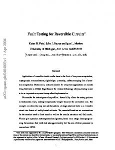
Fig. 1. Reversible circuit and its function representations
The remainder of this paper is structured as follows. The next section briefly reviews the core concepts of reversible circuits as well as the applied QMDD data-structure. Afterwards, Section III introduces the general idea as well as the main concepts of the proposed approach before the actual algorithm is described in detail in Section IV. Section V shows the correctness and completeness of the approach. Finally, Section VI reports experimental results, while Section VII concludes the paper and provides an outlook on future work.
II. BACKGROUND To keep this paper self-contained, the following section briefly reviews the basics on reversible functions and circuits. Afterwards, the QMDD data-structure is introduced which is utilized to compactly represent and synthesize reversible functions. A. Reversible Functions and Circuits A Boolean function f : IBr → IBr is reversible if it is bijective, i.e. if each input pattern is uniquely mapped to a corresponding output pattern. The synthesis problem is defined as the task of determining a reversible circuit for a given function f . Reversible circuits differ from conventional circuits, since e.g. fanout and feedback are not directly allowed [1]. Usually, they are built as a cascade of reversible gates including e.g. the Toffoli gate [11], the Fredkin gate [12], or the Peres gate [13]. In this paper, we focus on circuits composed of Toffoli gates. Definition 1 Let X = {x1 , . . . , xr } be a set of variables or lines. Then, a reversible circuit is described as a cascade g1 . . . gd . A gate gi = (Ci , ti ), i ∈ {1, . . . , d}, is a tuple of a set Ci ⊂ {x% | x ∈ X, % ∈ {−, +}} of (positive and negative) control lines and a target line ti ∈ X + with {t− i , ti } ∩ Ci = ∅. The target line ti of a Toffoli gate is inverted if and only if all positive (negative) control lines evaluate to one (zero). The values of all remaning lines are passed through the gate unaltered. That V is, the Toffoli gate maps (x1 , . . . , xti , . . . , xr ) to (x1 , . . . , x∈Ci x⊕x ˙ ti , . . . , x r ) with x˙ = x for any x+ and x˙ = x for any x− .
Example 1 Fig. 1(a) shows a reversible circuit with three lines and composed of four gates. The target lines are denoted by , while a represents a positive control line and a represents a negative control line. For example, assigning the input pattern 001 to the circuit results in the output pattern 101. Due to the reversibility, this computation can be performed in both directions. The cost of reversible circuits is usually measured by quantum cost as introduced by Barenco et al. in [14]. The quantum cost of a single reversible gate depends on the number of control lines. For example, a Toffoli gate with one or no positive control line has quantum cost of 1, while a Toffoli gate with two positive control lines has quantum cost of 5. In general, the quantum cost of a Toffoli gate with |Ci | positive control lines amount to at most 2|Ci |+1 − 3, i.e. this value increases exponentially in the worst case. If negative control lines occur, the same cost metric is applied except for the case where the Toffoli gate is entirely composed of negative controls. Then, the cost is increased by two [15]. Besides quantum cost, also the number of circuit lines is an important metric. Since for quantum computation each circuit line is represented by qubits, this value should be kept as small as possible. In this paper, we consider synthesis of reversible circuits with the minimal number of circuit lines. B. Quantum Multiple-valued Decision Diagrams Common canonical representations for reversible functions are truth tables and permutation matrices. In the following, these representations are briefly reviewed leading to the more compact QMDD data-structure which is utilized in this paper. A reversible function with r variables describes a permutation σ of the set {0, . . . , 2r − 1}. This permutation can also be described using a permutation matrix, i.e. a 2r × 2r matrix F = [fi,j ]2r ×2r with fi,j = 1 if i = σ(j) and 0 otherwise, for all i = 0, . . . , 2r − 1. That is, each column (row) of the matrix represents one possible input pattern (output pattern) of the function. If fi,j = 1, then the input pattern in column j maps to the output pattern in row i. Example 2 The truth table of the function realized by the circuit in Fig. 1(a) is given in Fig. 1(b). From this truth table, the permutation matrix shown in Fig. 1(c) is obtained.
x1 n
p0
n0
p
Fig. 2. QMDD and edge labels
As can be seen, the size of a permutation matrix grows exponentially with respect to the number of input/output variables. However, QMDDs [10] provide an efficient data-structure which enables a much more compact representation of permutation matrices. Definition 2 A QMDD is a directed acyclic graph composed of • two terminal vertices labeled by 0 and 1 representing the matrix [0]1×1 and the matrix [1]1×1 , respectively, and • non-terminal vertices labeled by a primary input xi and representing sub-matrices. The QMDD structure is based on recursively partitioning a 2r × 2r matrix F into four sub-matrices, each of dimension 2r−1 × 2r−1 . Accordingly, each non-terminal vertex has four outgoing labeled edges targeting child vertices representing from left to right (see also Fig. 2) • the top-left sub-matrix where xi maps from 0 to 0 (edge is denoted as negative and labeled n), • the top-right sub-matrix where xi maps from 1 to 0 (edge is denoted as pseudo-positive and labeled p0 ), • the bottom-left sub-matrix where xi maps from 0 to 1 (edge is denoted as pseudo-negative and labeled n0 ), and • the bottom-right sub-matrix where xi maps from 1 to 1 (edge is denoted as positive and labeled p). Equivalent sub-matrices are shared, i.e. the respective vertices have more than one parent. These basic concepts of QMDDs are clarified in the following example. Example 3 A QMDD representing the permutation matrix in Fig. 1(c) is shown in Fig. 1(d). For clarity, edges to a 0 terminal are indicated as stubs. The root vertex of this QMDD represents the overall matrix. Since this vertex is labeled with x1 , the child-vertices partition this matrix into four submatrices with respect to x1 . That is, the first successor represents all input/output mappings where x1 maps from 0 to 0 (i.e. the top-left sub-matrix is represented), the second successor represents all input/output mappings where x1 maps from 1 to 0 (i.e. the top-right sub-matrix is represented), and so on. Since the first and the fourth sub-matrix are equal (see shaded boxes in Fig. 1(c)), the respective vertices are shared. Furthermore, consider the leftmost vertex labeled with x2 representing the top-right sub-matrix. This vertex partitions this sub-matrix further (now with respect to x2 ). Since the last three sub-matrices of these vertices are entirely assigned to 0, the corresponding edges directly point to the 0 -terminal. A similar scheme is applied for all remaining vertices.
An important property of a QMDD is that all paths from the root vertex to an 1 -terminal have the same length and traverse the vertex labels in the same order. Thus, each of these paths can be referenced by the unique sequence of the traversed edge labels. Given a QMDD F , we call a path π from the root vertex to an 1 -terminal an 1-path and denote it as π ∈ F . An empty path is referred to as ε. Using 1-paths, the function represented by the QMDD can be determined as illustrated by the following example. Example 4 Consider again the QMDD depicted in Fig. 1(d). The path npn (marked bold starting from the first outgoing edge of x1 in Fig. 1(d)) represents the mapping of the input assignment 010 to the output assignment 010. Since no pseudo edges are in this path, the inputs and the outputs are equal. In contrast, the path p0 np0 (also marked bold in Fig. 1(d)) represents the mapping of the input assignment 101 to the output assignment 000. Here, a pseudo-positive mapping is applied to x1 and x3 , i.e. these values map from 1 to 0. This is consistent with the input/output mappings in the original truth table (see Fig. 1(b)) of that function. Overall, permutation matrices, and, therefore, reversible functions, can efficiently be represented using QMDDs. Moreover, e.g. due to the sharing of vertices, QMDDs are much more compact than exponentially large truth table- or matrixrepresentations. Thus, they enable the treatment of significantly larger functions. Furthermore, operations (e.g. the application of a Toffoli gate to a given function) can easily be performed on the QMDD data-structure. For a more detailed treatment on QMDDs, we refer to [10]. III. M AIN C ONCEPTS OF THE S YNTHESIS A PPROACH This section presents the main concepts of the proposed synthesis methodology including the general idea as well as the applied transformation rules. While this covers the basic concepts, the actual algorithm is provided in the next section. A. General Idea The task of the proposed synthesis approach is to determine a reversible circuit g1 . . . gd representing the function given in terms of a QMDD F . The respective gates of the desired circuit can be represented by permutation matrices and, thus, also by QMDDs T1 , . . . , Td . Since the composition of a reversible function with its inverse leads to the identity function (i.e. since F × F −1 = I), the synthesis problem can be formulated as the search for Toffoli gates T1 , . . . , Td so that F × Td × · · · × T1 = I. In other words, the main goal of the proposed synthesis approach is to determine a sequence of Toffoli gates so that their application to F leads to a QMDD representing the identity. Clearly, the determination of the respective Toffoli gates is crucial. However, the regular structure of a QMDD representing the identity can be exploited for this purpose. Consider for example Fig. 3 showing a QMDD representing the identity function over two variables. As can be seen, all p0 - and n0 edges of this QMDD point to the 0 -terminal, while all n- and p-edges always point to the same child vertex (this is because
x1
x1
x1 0 0
0 0
x2 (a) Before
0 0
Fig. 5. Structurally transforming a QMDD xi
1 Fig. 3. QMDD representing the identity matrix with two variables x1 x1
x1 0
0
1
x01
00
x1
x2
0 0
0 0
1
1
(a) Applying a NOT gate
(b) After
x1
x01
x2
x02
x2 0
xi
x1
xi n
00
x2 0
1
xi
xj
0 0
xj
xi p
p0
xi
xj
n
n0
(a) Swapping
p0
xj
p
n
n0
p
p0
n0
(b) Conditional swapping (pos.)
0 0
1
(b) Applying a CNOT gate
xi
xi
xj
xi
xj
xi
xi
xj
xj
xi
n
Fig. 4. Simple QMDD modifications n
only 0 to 0 and 1 to 1 mappings occur in an identity matrix). Accordingly, Toffoli gates should be determined in such a way that they establish this structure throughout a given QMDD F . Possible cases illustrating how this can be achieved are given in the following example.
0 0
xj p0
p n0
xj n
p0
p n0
xj
xj 0
0
0 0
p
n0
xj p
n 0 0
(c) Conditional swapping (neg.)
p
0
0 0p
0
xj 0
0
0
n00
(d) Shifting
Fig. 6. Reversible gates applied to QMDD vertices
In the following, we refer to these paths as follows: Example 5 Consider the QMDD on the left-hand side of Fig. 4(a) representing a 1 to 0 and a 0 to 1 mapping of x1 . In order to establish an identity structure, this needs to be transformed into a 1 to 1 and a 0 to 0 mapping of x1 . Since this is a simple inversion of the output values, a single NOT gate, i.e. a Toffoli gate (∅, x1 ), leads to the desired result. Furthermore, consider the QMDD on the left-hand side of Fig. 4(b). Here, the rightmost vertex labeled x2 needs to be “inverted” in order to achieve a QMDD representing the identity. However, simply applying a NOT gate as before does not work, since this would also affect the leftmost vertex labeled x2 . Thus, to directly address the respective vertex, control lines are applied. More precisely, a Toffoli gate ({x+ 1 }, x2 ) is added. Because of the positive control line, the inversion only applies if x1 is assigned the value 1, i.e. only for those vertices that are connected by a p- or p0 -edge to the parent vertex labeled x1 . Since the leftmost vertex is connected by an n-edge, this vertex remains unaltered. Overall, given a QMDD F , the general idea of the proposed approach is to apply Toffoli gates so that every vertex of F (as illustrated in Fig. 5(a)) is transformed into a corresponding identity structure (i.e. a vertex as illustrated in Fig. 5(b)). Then, the applied Toffoli gates can be composed into a circuit realizing F . While Example 5 only illustrated two special cases, generic transformation rules have been developed that establish the desired identity structure for any given QMDD. These rules are introduced in detail in the next section. B. Transformation Rules The purpose of the transformation rules is to transform any given � �QMDD vertex such that it represents the submatrix 0AB0 (see Fig. 5). Therefore, succeeding paths of a vertex either need to be swapped or shifted.
Definition 3 Let v be a vertex of a given QMDD. An e-path with e ∈ {n, p0 , n0 , p} is a path that starts in v with an e edge and results in the 1 -terminal. In order to perform the respective swaps and shiftings, two generic rules are sufficient. Rule 1 (Swapping) Applying a single NOT gate on line xi , i.e. a Toffoli gate without any control line as shown in Fig. 6(a), swaps all n- with p0 -paths as well as all p- with n0 -paths for each vertex labeled xi . In order to swap only the paths of a specific vertex v, positive and negative control lines are added according to the path from the root vertex to v. More precisely, each time a p- or p0 -edge is traversed a positive control line is added (see e.g. Fig. 6(b)) and each time an n- or n0 -edge is traversed a negative control line is added (see e.g. Fig. 6(c)). In the remainder of the paper, we refer to a path addressing a specific vertex v as µ. This rule has already been illustrated above in Example 5. Using the swapping rule, all paths that start in a vertex v are modified. However, often only selected paths should be modified (e.g. in the case where all succeeding paths point to a non-terminal and, thus, swapping is not sufficient to generate the identity structure). As a result, another rule is introduced which enables the shifting of specific paths only. Rule 2 (Shifting Rule) Similar to the swapping rule, also the shifting rule applies positive and negative control lines in order to address a specific vertex v of the QMDD. But to additionally address specific paths to be modified, also control lines according to these paths are added. More precisely, if xj is a label of a successive vertex of v, then adding a control line on line xj will shift only those paths who contain an outgoing por p0 -edge from vertices labeled xj . Analogously, adding a
µ=ε
0 0
µ=n µ=p
0 0
µ=nn µ=np µ=pn µ=pp
0
...
0
Fig. 7. Flow of the main algorithm
negative control line will consider only paths who contain an outgoing n- or n0 -edge. As an example, consider Fig. 6(d). The positive control line xj leads to a shifting of the second and the third path, since only these paths have either a p- or a p0 -edge starting from the xj -vertices. Furthermore, this principle can also be applied with more than one control line in order to address more selective paths. Note that the applied control lines will always affect two edges, i.e. p and p0 in case of a positive control line and n and n0 in case of a negative control line. However, it is sufficient to consider the n- and p0 -edges only. This is because after shifting e.g. all p0 -paths to the n-edge, not only the p0 -edge will point to the 0 -terminal, but also the corresponding n0 -edge. This is evidenced by the following theorem. �A B � Theorem 1 Let M be a permutation matrix M = C D of size 2r × 2r , such that A, B, C, D are of the same size, i.e. 2r−1 × 2r−1 . Then B (i.e. the sub-matrix represented by a p0 -edge) entirely is set to 0 if and only if C (i.e. the sub-matrix represented by an n0 -edge) entirely is set to 0. Proof. A permutation matrix has exactly one 1-element per row and column. If B = 0, then for each of the first 2r−1 rows, there must be a 1 in A and for each of the last 2r−1 rows, there must be a 1 in D. Since a binary unitary matrix does not contain more than 2r 1’s, C must be 0. The opposite direction follows analogously. � Based on the general concepts outlined above, the main flow of the proposed synthesis algorithm can be summarized. This is done in the next section. IV. A LGORITHM The formal algorithm of the proposed synthesis approach is described in the following. Afterwards, an example illustrates the application. Algorithm Q (QMDD-based synthesis). This algorithm outlines the main flow of the proposed approach. Q1. [Traverse graph.] Traverse the QMDD from the root vertex to the 1 -terminal in a breadth-first-manner. For each visited vertex v apply step Q2. Q2. [Apply transformations.] Transform v, such that the identity structure as in Fig. 5 results. This can be done by processing Algorithm P on v with µ being the path from the root vertex to v. Algorithm P is described in detail at the end of this section. It is important to understand the order in which the respective vertices are considered. For this purpose, consider Fig. 7 showing boxes illustrating (sub-)matrices to be considered by the algorithm. At the beginning, the algorithm considers the root vertex, i.e. the vertex representing the whole matrix (shadowed in Fig. 7). Applying Step Q2, the QMDD is transformed so that
this vertex is structured as shown in Fig. 5(b) (i.e. the p0 - and n0 -edge point to the 0 -terminal). As a result, only two succeeding vertices (representing the top-left and the bottom-right sub-matrix) are left to be considered (see second box in Fig. 7). In order to individually address them, positive and negative control lines are applied according to the µ-path as already illustrated in Rule 1 and incorporated in the transformation rules. As an example, in the second step of Fig. 7 the same algorithm is applied to the resulting two sub-matrices once by assigning µ to n and once by assigning µ to p. This process is recursively applied until all vertices have been transformed into the identity structure. The following definitions formalize the correlation between edges and control lines. Definition 4 (Signature of a path) Given a path π = e1 . . . er , the signature s(π) of that path is s1 . . . sr , where si = + if ei ∈ {p, p0 } and si = − otherwise. Definition 5 (Path controls) Given a path π = e1 . . . er and its signature s(π) = s1 . . . sr , the path controls c(π) for that path is the set {x%11 , . . . , x%r r }, where %i = si . Overall, due to the breadth-first-traversal, Step Q2 can exploit that the considered vertex v is always reached by p and n edges (as also illustrated in Fig. 7) and, thus, the application of Toffoli gates can be controlled by the corresponding c(µ). Having that, in each vertex v of a given QMDD the following Algorithm P used in Step Q2 is applied: Algorithm P (Shifting paths from p0 to n). This algorithm modifies a vertex v in a QMDD F such that its p0 -edge points to the 0 -terminal. Without loss of generality it is assumed that v is labeled xi and that v can be reached from the root vertex using a path µ consisting of n- and p-edges only. Let Πµ = {π | µπ ∈ F } be all paths in F from v to the 1 -terminal. P1. [Swap gate?] If |{π | p0 π ∈ Πµ }| > |{π | nπ ∈ Πµ }|, i.e. if there are more 1-paths going through the p0 -edge than through the n-edge, apply a Toffoli (c(µ), xi ) to F . P2. [Shift unique paths.] Let U = {π | p0 π ∈ Πµ ∧ 6 ∃ nπ 0 ∈ Πµ : s(π) = s(π 0 )} be all paths that go through p0 and have a signature that is not present via a path through n. For each π ∈ U , apply a Toffoli gate (c(µ) ∪ c(π), xi ) to F . P3. [Terminate?] If p0 points to a 0 -terminal, terminate. P4. [Unify a path.] Apply a gate that is controlled by at least c(µ) ∪ {x+ i } lines and a target on a successive vertex such that a path that starts with p0 can be made unique. Afterwards, return to step P2. After applying this algorithm, all p0 -paths of the considered vertex v are shifted to the n-edge (i.e. p0 does point to the 0 -terminal). Then, according to Theorem 1, also the n0 path of v is pointing to the 0 -terminal, i.e. the desired identity structure has been established and Algorithm Q can continue with the next vertex.
x1
x2
x2
000
000
x3 0
x1
0
00
x1
x1
x2
x2
x2
x2
000
x3
x3
00
x3 00
1
x1
x3 0
0
1
00
x1
x1
x2
x2
x2
x2
00
x3
x3
00
x3
x3
00
00
1
Fig. 8. Algorithm applied to the QMDD in Fig. 1(d)
Example 6 Fig. 8 illustrates the application of the proposed algorithm by means of the QMDD from Fig. 1(d). Starting at the root vertex, first this vertex is supposed to be transformed such that both, the p0 - and the n0 -edge point to the 0 -terminal. That is, all p0 -paths {p0 np0 , p0 nn0 } need to be shifted to the nedge. To address all these paths at once it is sufficient to set a negative control on line x2 , since each n-path, i.e. {npn, npp}, has a positive outgoing edge from x2 -vertices. As a result, ap0 plying a Toffoli gate ({x− 2 }, x1 ) shifts both p -paths at once to the n-edge resulting in the desired form for the root vertex (as depicted by means of the first arrow in Fig. 8). Afterwards, only the left vertex labeled with x3 has to be swapped. This vertex is reached via the path µ = nn representing the signature {−−}. Therefore, applying a Toffoli − gate ({x− 1 , x2 }, x3 ) finally leads to the QMDD representing the identity matrix as depicted on the right hand side of Fig. 8.
Hence, the algorithm to transform F to the QMDD representing the identity matrix using Toffoli gates is complete. � The algorithm is correct by construction since the QMDD is transformed in each step according to the applied gate. If the identity matrix results, than the sequence of gates represent a reversible circuit realizing the initial function. VI. E XPERIMENTAL E VALUATION
In this section the completeness and the correctness of the algorithm is shown.
The QMDD-based synthesis method as introduced above has been implemented in C++ and evaluated on different benchmark functions. In this section, the obtained results are presented. We distinguish between two evaluations. First, the results obtained by the proposed approach are compared to previous work, namely the transformation-based synthesis method [5] and the BDD-based synthesis method [7]2 . Afterwards, results showing the scalability of the proposed approach are discussed. All experiments have been conducted on a 2.66 GHz Intel Core 2 Duo processor with 3 GB of main memory running Linux 2.6. The timeout was set to 2 000 CPU seconds.
Theorem 2 The algorithm described in Section IV terminates for each QMDD F that represents a permutation matrix.
A. Comparison to Previous Synthesis Approaches
V. C OMPLETENESS AND C ORRECTNESS
Proof. We assume that Algorithm P terminates and first prove that the main algorithm terminates under that condition. A QMDD consists of a finite number of vertices. Therefore, also the number of vertices per level is finite. It is sufficient to show, that once a vertex is brought to the form that its p0 and n0 edge point to the 0 -terminal, this will not be changed by successive steps. Algorithm P sets target lines only on the considered vertex v or on successive vertices. Since all gates are controlled at least by the signature of µ, no other vertex which is at the same level as v is transformed by this. Since additionally a breadth-first traversal is performed, already considered vertices are never modified afterwards. It is left to show that Algorithm P terminates. The Steps 1 to 3 of Algorithm P are straightforward. Therefore, it remains to prove that a path going through p0 can always be made unique. There must be a signature s that is not represented by a path going through n, since if that would be the case according to Theorem 1 p0 must point already to 0 . Controlling the gate with x+ i in that step prohibits paths from being changed going through the n edge. Setting a positive control line on the respective line from vertex v can thus transform the paths going through p0 independently, resulting in a path representing signature s.
Both the transformation-based method [5] and the BDDbased method [7] represent state-of-the-art synthesis approaches with respective pros and cons (e.g. minimal number of circuit lines but poor scalability in case of the transformation-based approach versus low quantum cost and good scalability but a large number of circuit lines in case of the BDD-based approach). The proposed QMDD-based synthesis approach provides a promising compromise between these contradictory properties. In order to show this, all three approaches have been experimentally compared by means of a set of benchmark functions taken from RevLib [17]. The results are presented in Table I. The first column denotes the name of the respective benchmark. Afterwards, the number of lines (r), the number of gates (d), and the quantum cost (QC) of the circuits obtained by the respective synthesis approaches are reported. Column t denotes the run-time in seconds required to generate these results. The columns ∆QCTBS and ∆QCBDD report the absolute difference of the quantum cost measured for the circuits obtained by the transformation-based method and by 2 In order to conduct these comparisons, we applied the implementations of these approaches as provided by RevKit [16].
TABLE I C OMPARISON TO PREVIOUS SYNTHESIS APPROACHES Benchmark max46 rd73 sqn sym9 dc1 wim z4 cm152a cycle10 2 plus63mod4096 rd84 sqrt8 adr4 dist plus127mod8192 plus63mod8192 radd root squar5 clip cm42a cm85a pm1 sao2 co14 dc2 misex1
r 10 10 10 10 11 11 11 12 12 12 12 12 13 13 13 13 13 13 13 14 14 14 14 14 15 15 15
Transformation-based [5] d QC t 284 11977 0.04 208 5889 0.03 216 7467 0.03 231 4606 0.03 247 12123 0.04 753 32556 0.09 74 1069 0.04 33 409 0.06 19 1179 0.04 384 27274 0.12 381 12117 0.11 1024 55095 0.23 199 5195 0.16 741 47281 0.32 769 58352 0.35 447 38070 0.25 432 17074 0.24 1000 59054 0.39 83 1967 0.13 1304 111525 0.88 2010 176497 1.21 625 29560 0.56 2010 176497 1.2 1176 101535 1.06 8270 617906 13.68 803 43522 1.19 1358 111286 2.4
r 60 26 47 28 28 25 26 16 39 23 37 31 33 94 25 25 21 79 36 97 32 34 32 76 28 65 39
BDD-based [7] d QC 191 575 85 229 160 484 69 213 77 193 62 134 75 187 24 68 78 202 49 89 114 314 95 259 93 237 331 1023 54 98 53 97 55 95 277 857 99 267 368 1196 79 151 78 222 79 151 237 725 76 172 197 585 103 283
t 0.02 0.02 0.01 0.02 0.03 0.04 0.04 0.07 0.07 0.07 0.08 0.08 0.19 0.2 0.17 0.17 0.17 0.2 0.18 0.45 0.44 0.38 0.45 0.35 0.75 0.98 0.99
r 10 10 10 10 11 11 11 12 12 12 12 12 13 13 13 13 13 13 13 14 14 14 14 14 15 15 15
QMDD-based d QC 51 42248 147 13858 50 3507 72 59168 25 426 13 239 59 3621 8 208 36 10684 26 5413 278 33900 55 3923 75 5125 241 20624 27 9148 32 10282 75 5125 204 18497 30 704 232 22495 10 260 99 13368 10 260 63 9018 14 458710 60 2974 35 1000
t 0.03 0.04 0.03 0.04 0.02 0.03 0.05 0.02 0.07 0.04 0.16 0.07 0.15 0.31 0.1 0.1 0.17 0.27 0.13 0.48 0.24 0.24 0.24 0.27 0.24 0.56 0.74
∆QCTBS 30271 7969 -3960 54562 -11697 -32317 2552 -201 9505 -21861 21783 -51172 -70 -26657 -49204 -27788 -11949 -40557 -1263 -89030 -176237 -16192 -176237 -92517 -159196 -40548 -110286
∆QCBDD 41673 13629 3023 58955 233 105 3434 140 10482 5324 33586 3664 4888 19601 9050 10185 5030 17640 437 21299 109 13146 109 8293 458538 2389 717
∆rBDD -50 -16 -37 -18 -17 -14 -15 -4 -27 -11 -25 -19 -20 -81 -12 -12 -8 -66 -23 -83 -18 -20 -18 -62 -13 -50 -24
r: Number of lines d: Number of gates QC: Quantum cost t: Run-time ∆QCTBS (∆QCBDD ): Difference of the QC for circuits obtained by the QMDD-based method and the transformation-based method (BDD-based method)
the BDD-based method, respectively, compared to the circuits obtained by the proposed QMDD-based method. Finally, column ∆rBDD reports the differences in the number of circuit lines between the BDD-based method and their minimal value (as ensured by both, the transformation-based and the QMDDbased method). First of all, it can be seen that run-time is not a crucial factor. If the respective data-structure (i.e. the truth-table, the BDD, or the QMDD) can be built, all synthesis approaches generate the respective circuits very fast. However, the quality of the results vary significantly. Obviously, the BDD leads to the best results with respect to quantum cost. But this comes at a high price: a very large number of circuit lines which is way beyond the optimum. In particular in the domain of quantum computation, where circuit lines are represented by qubits, this is crucial. In contrast, both the transformation-based synthesis approach and the QMDD-based synthesis approach lead to circuits with the minimal number of circuit lines. As a consequence, larger quantum cost have to be accepted3 . But applying the proposed QMDD-based method, this amount can significantly be reduced. In fact, on average circuits with 50% less quantum cost are generated in comparison to the transformation-based approach. Besides that, the QMDDbased method provides much better scalability as shown in the next section.
3 This already has been observed before in [18] for small functions. Here, significant differences in the quantum cost have been observed already between circuits with the minimal number of lines and circuits with just one or two additional lines.
B. Scalability of the QMDD-based Method So far, no synthesis approach for large functions has been proposed which ensures the minimality of the number of circuit lines. Accordingly, no established benchmark set including large reversible benchmarks is available. Because of this, we show the scalability of the proposed QMDD-based method by means of structural examples (including the toffoli and the graycode function as well as arithmetic operations such as the adder, the increase module, or the multiplier) enriched by a set of automatically generated random functions. Since all these functions cannot efficiently be processed by the transformation-based method anymore (assuming a timeout of 2 000 CPU seconds), only the results obtained by the QMDDbased method are discussed in the following. The results are presented in Table II. Again, the columns denote the number of lines (r), the number of gates (d), the quantum cost (QC) of the obtained circuits as well the runtime (t) required to generate the respective results. As can be seen, functions including up to 100 variables can automatically be synthesized with the minimal number of circuit lines. The run-time varies depending on the respective benchmark. While for example the increase operation or the graycode function can be generated very efficiently, random functions or the mutliplier do not perform that well. However, it is left for future work to (theoretically) analyze for which functions QMDDs perform well or not. At this point, we assume that, similar to BDDs [19], different classes of functions exist that either show a positive or a negative behavior with respect to their synthesis capability. Overall, the QMDD-based method is the first automatic synthesis approach which is applicable to larger functions and at the same time guarantees the minimal number of circuit lines.
TABLE II S CALABILITY OF THE QMDD- BASED METHOD Benchmark adder9 random1412 random1752 random1242 random1536 multiplier5 adder10 random1706 random1739 random1795 random1434 random1865 random1383 random1475 random1543 random1915 random1369 adder11 random1862 random1371 multiplier6 random1201 random1937
r d 18 3595 20 167 20 15 20 1203 20 4 20 11510 20 8204 21 16 21 9408 21 37 21 23 21 16 22 2415 22 1902 22 2209 22 69 22 16 22 18445 22 16 23 312880 24 68241 25 9070 25 19 r: Number of lines QC: Quantum cost
QC 67768365 4219884 195 104323 804 2241224 538649284 608 1419008 1975 918 608 464628 281594 338220 4196 800 > 4294967296 800 100299312 17212234 3646604 908
t 56.69 41.15 29.74 48.73 20.35 29.71 311.21 46.49 4.75 38.53 32.99 46.48 184.31 138.67 206.72 80.34 71.41 1677.82 50.91 489.52 794.38 972.20 900.31
VII. C ONCLUSIONS AND F UTURE W ORK Ensuring the minimal number of circuit lines during synthesis of reversible circuits is crucial. However, existing synthesis approaches are either only applicable to small functions or lead to circuits that are way beyond the minimum of the lines. In this paper, we proposed a complementary method which overcomes these limitations. Therefore, QMDDs are utilized, that serve as an ideal data-structure to efficiently store and manipulate reversible functions. Given a QMDD representing the function to be synthesized, Toffoli gates are applied so that every vertex of the QMDD is transformed into an identity structure. Afterwards, the applied Toffoli gates are composed to a circuit realizing the desired function. Experimental results showed that in comparison to similar approaches, circuits with 50% less quantum cost result on average. Furthermore, circuits with the minimal number of lines can automatically be realized for the first time for large functions. In this sense, the proposed approach provides a new synthesis methodology that also builds the basis for further research. In particular, future work will focus on the theoretical analysis of the proposed approach. As shown in the experimental evaluations, some functions can efficiently be realized using the QMDD methods while other functions do not perform that well. Besides that, also the direct application of the presented ideas to quantum circuits is promising. However, although QMDDs are also capable to represent dedicated quantum operations, the corresponding transformation rules are much harder to develop. ACKNOWLEDGMENTS We would like to thank D. Michael Miller for providing us with an implementation of the QMDD package introduced in [10]. This work was supported by the German Research Foundation (DFG) (DR 287/20-1). R EFERENCES [1] M. A. Nielsen and I. L. Chuang, Quantum Computation and Quantum Information. New York, NY, USA: Cambridge University Press, Oct. 2000. [2] R. Landauer, “Irreversibility and Heat Generation in the Computing Process,” IBM Journal of Research and Development, vol. 5, no. 3, pp. 183– 191, July 1961.
Benchmark random1267 graycode40 increaser40 toffoli40 toffoli50 graycode50 increaser50 increaser60 toffoli60 graycode60 increaser70 toffoli70 graycode70 graycode80 toffoli80 increaser80 graycode90 toffoli90 increaser90 graycode100 increaser100 toffoli100
r 26 40 40 40 50 50 50 60 60 60 70 70 70 80 80 80 90 90 90 100 100 100
d 238 39 39 1 1 49 49 59 1 59 69 1 69 79 1 79 89 1 89 99 99 1
> > > > > > > > > > > > > >
QC 20122 39 4294967296 4294967296 4294967296 49 4294967296 4294967296 4294967296 59 4294967296 4294967296 69 79 4294967296 4294967296 89 4294967296 4294967296 99 4294967296 4294967296
t 1942.24 0.00 0.05 0.00 0.01 0.00 0.09 0.13 0.00 0.01 0.19 0.00 0.01 0.01 0.00 0.32 0.01 0.00 0.45 0.01 0.69 0.01
d: Number of gates t: Run-time
[3] C. H. Bennett, “Logical Reversibility of Computation,” IBM Journal of Research and Development, vol. 17, no. 6, pp. 525–532, Nov. 1973. [4] V. Shende, A. Prasad, I. Markov, and J. Hayes, “Synthesis of reversible logic circuits,” IEEE Trans. on CAD, vol. 22, no. 6, pp. 710 – 722, June 2003. [5] D. M. Miller, D. Maslov, and G. W. Dueck, “A transformation based algorithm for reversible logic synthesis,” in Design Automation Conference. ACM, June 2003, pp. 318–323. [6] K. Fazel, M. Thornton, and J. Rice, “ESOP-based Toffoli Gate Cascade Generation,” in IEEE Pacific Rim Conf. on Communications, Computers and Signal Processing. IEEE, Aug. 2007, pp. 206–209. [7] R. Wille and R. Drechsler, “BDD-based synthesis of reversible logic for large functions,” in Design Automation Conference. ACM, July 2009, pp. 270–275. [8] R. Wille, O. Kesz¨ocze, and R. Drechsler, “Determining the Minimal Number of Lines for Large Reversible Circuits,” in Design, Automation and Test in Europe. IEEE Computer Society, Mar. 2011, pp. 1204– 1207. [9] R. Wille, M. Soeken, and R. Drechsler, “Reducing the number of lines in reversible circuits,” in Design Automation Conference. ACM, June 2010, pp. 647–652. [10] D. M. Miller and M. A. Thornton, “QMDD: A Decision Diagram Structure for Reversible and Quantum Circuits,” in Int’l Symp. on MultipleValued Logic. IEEE Computer Society, May 2006, pp. 30–30. [11] T. Toffoli, “Reversible computing,” in Automata, Languages and Programming, ser. Lecture Notes in Computer Science, J. W. de Bakker and J. van Leeuwen, Eds., vol. 85. Springer, July 1980, pp. 632–644. [12] E. Fredkin and T. Toffoli, “Conservative logic,” Int’l Journal of Theoretical Physics, vol. 21, no. 3, pp. 219–253, Apr. 1982. [13] A. Peres, “Reversible logic and quantum computers,” Phys. Rev. A, vol. 32, no. 6, pp. 3266–3276, Dec. 1985. [14] A. Barenco, C. H. Bennett, R. Cleve, D. P. DiVincenzo, N. Margolus, P. Shor, T. Sleator, J. A. Smolin, and H. Weinfurter, “Elementary gates for quantum computation,” Phys. Rev. A, vol. 52, no. 5, pp. 3457–3467, Nov. 1995. [15] D. Maslov, G. W. Dueck, D. M. Miller, and C. Negrevergne, “Quantum Circuit Simplification and Level Compaction,” IEEE Trans. on CAD, vol. 27, no. 3, pp. 436–444, Mar. 2008. [16] M. Soeken, S. Frehse, R. Wille, and R. Drechsler, “RevKit: A Toolkit for Reversible Circuit Design,” in Workshop on Reversible Computation, July 2010, pp. 69–72, RevKit is available at www.revkit.org. [17] R. Wille, D. Große, L. Teuber, G. W. Dueck, and R. Drechsler, “RevLib: An Online Resource for Reversible Functions and Reversible Circuits,” in Int’l Symp. on Multiple-Valued Logic. IEEE Computer Society, May 2008, pp. 220–225. [18] D. M. Miller, R. Wille, and R. Drechsler, “Reducing reversible circuit cost by adding lines,” in Int’l Symp. on Multiple-Valued Logic, May 2010, pp. 217–222. [19] R. E. Bryant, “Graph-Based Algorithms for Boolean Function Manipulation,” IEEE Trans. on Computers, vol. C-35, no. 8, Aug. 1986.