â¡University of Karlsruhe, Institute of Computer Science and Engineering ... technology can be used to generate complex humanoid robot motions that may require a great ..... Robotics and Automation, Orlando, Florida, 2006, pp. 2561â2567.
Synthesizing Goal-Directed Actions from a Library of Example Movements Aleˇs Ude∗† , Marcia Riley¶ , Bojan Nemec∗ , Andrej Kos∗ , Tamim Asfour‡ and Gordon Cheng†§ ∗ Joˇzef † ATR
Stefan Institute, Dept. of Automatics, Biocybernetics and Robotics Jamova 39, 1000 Ljubljana, Slovenia
Computational Neuroscience Laboratories, Department of Humanoid Robotics and Computational Neuroscience 2-2-2 Hikaridai, Seika-cho, Soraku-gun, Kyoto 619-0288, Japan ‡ University
of Karlsruhe, Institute of Computer Science and Engineering c/o Technologiefabrik, Haid-und-Neu-Str. 7, 76131 Karlsruhe, Germany
§ Japan
Science and Technology Agency, ICORP Computational Brain Project 4-1-8 Honcho, Kawaguchi, Saitama, Japan ¶ Georgia
Institute of Technology, College of Computing Atlanta, Georgia 30332–0250, USA
Abstract— We present a new learning framework for synthesizing goal-directed actions from example movements. The approach is based on the memorization of training data and locally weighted regression to compute suitable movements for a large range of situations. The proposed method avoids making specific assumptions about an adequate representation of the task. Instead, we use a general representation based on fifth order splines. The data used for learning comes either from the observation of events in the Cartesian space or from the actual movement execution on the robot. Thus it informs us about the appropriate motion in the example situations. We show that by applying locally weighted regression to such data, we can generate actions having proper dynamics to solve the given task. To test the validity of the approach, we present simulation results under various conditions as well as experiments on a real robot.
I. I NTRODUCTION Humanoid robotics has dealt with the problem of learning complex humanoid behaviors for a long time. It was soon realized that to overcome problems arising from high dimensional and continuous perception-action spaces, it is necessary to guide the search process, thus effectively reducing the search space, and also to develop higher-level representations suitable for faster learning. To achieve these goals, researchers in sensorimotor learning have explored various solutions. Some of the most notable among those are learning from demonstration (or imitation learning) and motor primitives. Building on the large body of work by the computer graphics community, it has been shown that motion capture technology can be used to generate complex humanoid robot motions that may require a great deal of skills and practicing to be realized, e. g. dancing [11], [18], [19]. Techniques to adapt the generated movements with respect to various robot constraints have also been proposed [10], including more complex constraints such as self-collision avoidance and balancing of a free standing dancing robot [8], [14]. Dynamics filter
that can create a physically consistent motion from motion capture data has also been proposed [22]. While these works can overcome the problem of different embodiments of the robot and the demonstrator, they do not deal with the effects of motion acting on the external world. Different methods are needed to adapt the captured motions to the changes in the external world and synthesize goal-directed actions, such as in the case of object manipulation tasks. In tasks involving the manipulation of objects, it is necessary to adapt the observed movements to the current state of the 3-D world. For any given situation, it is highly unlikely that an appropriate movement would be observed in advance and included in the library. While many tasks can be learned assuming a proper representation for the physics of the task, such an approach relies on a priori knowledge about the action and therefore does not solve the complete learning problem. To avoid specifying the physical model of the task, Miyamoto et al. [9] based their methodology on programming by demonstration and derived a representation for optimal trajectories, which they referred to as via-points. They were able to teach a robotic arm a fairly difficult game of Kendama and tennis serves. Schaal et al. [5], [17] proposed a more general nonparametric approach based on nonlinear dynamic systems as policy primitives. They developed canonical equations for rhythmic and discrete movements and demonstrated that these systems can be used to learn tasks such as tennis strokes and drumming. Hidden Markov models (HMMs) are another popular methodology to encode and generalize the observed movements [1], [3], [6]. While techniques that enable the reproduction of generalized movements from multiple demonstrations have been proposed, generalization across movements to attain an external goal of the task is not central to these works. HMMs, however, can be used effectively for motion and situation recognition [6] and to determine which control variables should be imitated and how [3].
Fig. 1.
Human demonstration of the ball throw, unsuccessful direct reproduction on a humanoid robot, and a successful action execution after coaching
The computer graphics community has also studied human motion synthesis from example movements. The most common approach is to generalize across a number of movements by linear interpolation, like e. g. [21]. If done correctly, such an approach results in physically correct movements under many circumstances [15]. Rose et al. [13] represent the motions by B-splines and use radial basis functions to interpolate between the control points of B-Splines. Automatic re-timing of the captured movements based on registration curves has also been considered [7]. Most of the early works dealt with the intepolation of relatively short movements, but interpolation of longer action sequences is also possible as shown in [16]. While these works address many problems relevant to the robotics community, their main aim is to generate realistic computer animations. Our focus, however, is to show that movement interpolation can generate actions that can change the external world in such a way that the goal of an action is attained. In order words, we focus on the synthesis of goal-directed actions and how to make action synthesis from example movements applicable for the implementation on a real robotic system. In the following we propose a new movement generalization methodology based on locally weighted regression [2]. The goal of an action is used to index into the library of stored movements. We also briefly deal with different approaches that can be applied to generate a suitable movement library. We show both in simulation and on a real robot that the proposed approach can be used to synthesize goal-directed actions. As a test example we use the task of throwing a ball into a basket, which has the advantage that its physics is well understood and we can thus compare our results with an ideal system. II. C OLLECTING THE E XAMPLE M OVEMENT L IBRARY As mentioned in the introduction, motion capture has been used successfully to generate fairly complex movements on a
humanoid robot. However, direct reproduction of movements, even if it includes the physical constraints of a robot, rarely results in a successful execution of the task that involves external goals. In the throwing example of Fig. 1, the direct reproduction ended up in a throw that missed the basket (middle row of figures). Moreover, the execution of the throwing movement was suboptimal in many other ways such as for example timing of the ball release and smoothness. It was therefore necessary to develop a methodology to adapt the initial robot motion. In our previous work, we explored the coaching paradigm to solve these problems. Coaching provides a familiar setting to most people for interacting with and directing the behavior of a complex humanoid robot where human-robot communication takes the form of coach’s demonstrations and high-level qualitative instructions. In this way it is possible to generate throwing movements that result in successful throws with good dynamical properties, which are suitable for generalization. See [12] for more details. There are other ways than coaching to adapt captured movements to attain the goal of the task in a given situation. The viapoint representation based on the forward-inverse relaxation neural network model (FIRM) [20] is one of them. Via points are extracted sequentially by taking the first two via-points to be the end-points of the movement and interpolating the movement using the minimum principle for the approximated dynamics model (point mass), which results in a minimum jerk trajectory (fifth order polynomial). New via-points are determined by calculating the distance between the observed and interpolated trajectory and adding the via-points at the point of the maximum squared error until the error is small enough. Hovewer, the movement generated by the final set of via-points still cannot ensure the successful execution of the task. It was therefore proposed to adapt the trajectory by moving the via-points until the robot is successful [9]. This is
accomplished by constructing a function from via-points to the task goal and by moving the via-points using a Newton-like optimization method. In certain situations, it is well possible that a skilled engineer would be able to design optimal trajectories for some situations. The coaching paradigm described above just provides the technology that enables non-skilled people to design ”good” movements for learning. Thus, all these methods for trajectories generation can be utilized for the construction of a library of movements. The method we propose in the following is independent of the data collection method1 . III. G ENERALIZATION ACROSS M OVEMENTS The data collection mechanisms described in the previous section provide us with a set of movements M i , i = 1, . . . , N umEx, that were executed by the robot and succeeded to accomplish the goal of the task in the observed situations. We denote the goals by q i ∈ Rm , i = 1, . . . , N umEx. In the case of throwing a ball into a basket, the goals {q i } are specified by the positions of the basket. Every movement M i is encoded by a sequence of trajectory points pij at times tij , j = 1, . . . , ni . We have experimented both with endeffector trajectories (in this case pij are points in the Cartesian space) and with robot joint trajectories (in this case pij are the joint angles stemming from the active degrees of freedom). Our aim is to develop a method that can compute motions that attain the goal of the task for any given query point (goal) q. To find a representation for the desired movements, we follow [9], [20] and represent the trajectories by fifth order splines. Due to their local support property, we chose B-splines [4] to implement the spline functions, which results in the following representation ! M (t) = bk Bk (t), (1) k
where Bk are the basis functions from the selected B-spline basis. A. Determination of Basis B-Spline Functions
We adapted the via-point approach of [9] to find a good spline basis. Unlike [9], which deals with only one example movement, we need to consider multiple examples. We therefore introduce what we call common knot points. Common knot points are extracted sequentially as follows: 1) First all trajectories are time-scaled to interval [0, 1]. The duration of every movement Ti is also stored with each example. Without re-timing it is not possible to interpolate between the examples. See Section III-C for more details on this issue. The initial knot sequence for the fifth order spline is taken to be K1 = {0, 0, 0, 0, 0, 0, 1, 1, 1, 1, 1, 1}, which results in a so called clamped spline. Clamped splines can be used to calculate minimum jerk splines interpolating the desired position, velocity, and acceleration at the end points (0 1 However, a via-point like method is used to obtain a suitable representation for goal-directed actions.
and 1). The initial spline basis consists of six basis functions. 2) For every movement M i we determine the best approximating fifth order spline S li with basis functions defined by the current knot sequence Kl . 3) For all configurations (pij , sij ), sij = tij /Ti , we calculate the distance to the generated spline trajectories elij = "pij − S li (sij )".
(2)
Kl+1 = {0, . . . , sij , . . . , 1}.
(3)
We select the knot point to be added to the existing knot sequence at the point of the maximum squared error elij between the example movements and the generated spline trajectories. The new knot sequence is given by
4) The procedure continues at step 2 (with l ← l + 1) until the difference between the example movements and the generated spline trajectories becomes sufficiently small. The above process is similar to the way Miyamoto et al. [9] determine via-points. Its final result, the knot sequence KL , is applied to define a spline that we use to synthesize goaldirected actions. B. Synthesizing New Actions Given a goal q, we would like to find movement M(q) that can attain this goal. Using the above representation we can write N ! M (q) = bk (q)Bk , (4) k=1
where N is the number of B-spline basis functions defined by the knot sequence KL . In computer graphics, new movements are often synthesized by simply interpolating the splines approximating the example movements [15] ! M= wi M i . (5) i
However, if the approximation by splines is not accurate, such an approach can introduce undesired deformations in the example movements, which can affect the synthesized actions. We therefore studied other techniques such as locally weighted regression [2] to generate movements for any given goal. Our main motivation is that it is difficult to find global models that are valid everywhere and that it is therefore better to look for local models that are correct only in one particular situation, but are easier to compute. In locally weighted regression, local models are fit to nearby data. Its application results in the following optimization problem M (q) = arg min{C(q)}, b "2 "N ni " ! N umEx " ! ! " " bk Bk (sij ) − pij " W (di (q, qi )) . C(q) = " " " i=1 j=1 k=1 (6) Here W is the weighting kernel function and di are the distance functions between the query point and the data points
qi . The unknown parameters we minimize over are b = [bT1 , . . . , bTN ]T . Since W (di (q, qi )) does not depend on the B-spline coefficients bk , the optimization problem (6) is a classic linear least squares problem. It is, however, very large because it contains all data points pij describing the example movements. Before describing how to solve it, we define distance functions di and the kernel function W. We take the weighted Euclidean distance for di , i. e. di (q, qi ) =
1 "q − qi ", ai > 0. ai
(7)
It is best to select ai so that there is some overlap between the neighboring query points. One possibility is ai = 2 min "qi − qj " j
(8)
By selecting ai in this way we ensure that as query points transition from one data point to another, the generated movements also transition between example movements associated with the data points. There are many possibilities to define the weighting function W [2]. We chose the tricube kernel # (1 − |d|3 )3 if|d| < 1 W(d) = (9) 0 otherwise
This kernel has finite extent and continuous first and second derivative. Combined with distance (7), these two functions determine how much influence each of the example movements M i has. It is easy to see that the influence of each M i diminishes with the distance of the query point q from the data point q i . If the data points q i are distributed uniformly along the coordinate axes, then every new goal directed movement M (q), q %= q i , will be influenced by 4m example movements2 , where m is the dimension of the query point. Optimization of criterion (6) is a linear least-squares problem. Locally weighted regression combined with the local support of B-spline basis functions make the resulting linear system that needs to be resolved sparse. Additionally, since only the weights and not the basis functions depend on the query point q, the sparse system matrix can be precomputed in its entirety. We applied the Matlab implementation of sparse matrix algebra to solve the resulting linear problems, which enabled us to generate new actions quickly despite the large number of trajectory points pij . Another advantage of the proposed method is that there is no need to search for nearby movments in the database; locally weighted regression and sparse matrix algebra do this job. C. Re-Timing of the Generated Actions To interpolate between example movements, we needed to first scale the timing of all trajectories to a common interval, which we chose to be [0, 1]. This scaling, however, causes the velocities and accelerations of both the example movements and the synthesized actions to be scaled. To synthesize 2 Exception
are the movements at the edge of the training space.
movements with proper velocities and accelerations – which is essential to solve dynamic tasks – we need to rescale the resulting actions back to the original time interval. As described in Section III-A, the timing of each example motion M i is scaled by 1/Ti , where Ti is the duration of the example movement. Hence to re-time the synthesized action, we need to compute an estimate for the expected time duration T . For this purpose, we approximate the expected timing by a multivariate B-spline function ft : Rm → R, which is estimated by minimizing the following criterion N umEx ! i=1
2
(ft (q i ) − Ti ) .
(10)
In our experiments we defined a B-spline basis by uniformly subdiving the domain of the goal points q i . A suitable timing for the synthesized action is then given by T = ft (q) =
M !
ai Bi (q).
(11)
i=1
Finally, the correctly timed trajectories for the synthesized actions obtained by minimizing criterion (6) can be calculated by mapping the knot points KL = si to the new knot sequence KL! KL! = {0, . . . , T ∗ si , . . . , T }. (12)
The optimal coefficients bk (q) remain unchanged and the spline with these coefficients defined on the knot sequence KL! specifies an action with appropriate velocities and accelerations. It should be noted here that uniform scaling might not be suitable for every task. In some situations it might be more appropriate to segment the example movements and apply different scaling factors to different time intervals. Here matching of key events is crucial for good results [15]. Computer graphics community has proposed some approaches to automatically resolve this problem [7], [13]. Since the task considered in this paper does not require nonuniform scaling, we did not attempt to develop more complex re-timing methods here. IV. E XPERIMENTAL R ESULTS We validated our approach both in simulation and on the real robot. As a test example we considered the task of throwing a ball into a basket, which has the advantage that it is a dynamic task, dependent not only on the positional part of the movement, and that its physics is well understood. This allows us to compare our results with an ideal system. It can easily be shown that the trajectory of the ball after the release is fully specified by the position and velocity at the release point gt2 , (13) 2 where (x0 , y0 ) is the release point, v0 is the linear velocity of the ball at release time and α is the initial angle of the throw. We considered the problem where the target basket is placed x = x0 + v0 t cos(α), y = y0 + v0 t sin(α) −
in xy-plane. Note that a humanoid robot could normally turn towards the basket, thus solving this problem allows the robot to throw the ball to any position in space.
0.15
A. Simulation Results error (m)
0.1
For the interpolation to work, the style of example movements must be similar. Interpolation between movements that have nothing in common would not results in sensible actions. To generate examples that can be used for action synthesis, we used Eq. (13) to design Cartesian space trajectories that theoretically result in successful throws for a given basket position. The base of the robot, which was taken to be a seven degrees of freedom arm, was fixed in space. The designed trajectories consisted of circular and linear parts. From a given basket position, we determined a suitable release point and by specifying the desired angle under which the ball should fall into a basket (taken to be 60 degrees), a good trajectory for each situation could be calculated. We distributed the goal basket positions within a rectangular area of size 4 × 2 meter squares, with the lower left corner positioned at (1.2, 0.1) meters. The base of the robot was placed at (−0.5, 0.1) meters. Fig. 2 shows the velocity profiles of the movements generated by specifying a grid in thin rectangular area with baskets placed every 0.5 meters (altogether 45 basket positions). We used inverse kinematics to generate example trajectories in joint space. By specifying different grid sizes for training (we took grid side lenghts of 0.25, 0.5, and 1 meter, which resulted in 15, 45, and 153 example movements within the training area), we tested how many example movements are necessary to throw a ball anywhere within the training area with good precision. Tables I and II show the errors in the synthesized throws. They were calculated by using Eq. (13) to determine the ball flight trajectory after release. All values in the tables are given in centimeters. The density of the training data is specified by the grid size (rightmost column). Since the error was smaller away from the edges of the library (see Fig. 3), we estimated
0.05
0 5 4
2
3
1.5 2
1 1
0.5
x position (m)
y position (m)
Fig. 3. The throw error. The graph corresponds to the condition of Tab. I with grid size 50 × 50, joint space synthesis. The error is larger at the edges of the training area where less data is available for synthesis.
the error in the complete training area and in the area reduced by the side length of the grid along the edges. In Tab. I the data points pij used in (6) consisted of both positions and velocities3 , which were approximated by the spline functions. In Tab. II the data points pij consisted of positional information only. To test the method we evaluated the throws by applying a grid of 2.5×2.5 centimeter squares, which resulted in 13041 test throws for every training condition. Both tables show that the accuracy of the ball throw is significantly improved when more data is available. We achieved average precision between 1 and 2.5 cm for the two finer grids. Hence, 45 training examples were enough for an average precision of below 2 cm within the reduced area. The comparison of Tab. I and II also shows that the explicit addition of velocity information did not improve the throwing precision. We believe that the main reason for this is that our data was simulated at a typical robot servo rate of 500 Hz, 3 Formula (6) is valid for positional information only, but extension to velocities and accelerations is straightforward and does not significantly change the linear system that needs to be resolved.
9
7
1
6
0.8 time (sec)
Velocities (m/sec)
8
5 4
0.6 0.4
3 0.2 0
2
2.5 2
2
1
1.5 1
4 0.5
0 !1
6 x position (m)
0
200
Fig. 2.
400
600 800 Time (milliseconds)
1000
Cartesian velocities of example movements
0
y position (m)
1200
Fig. 4. Spline function approximating the release times of the movements with respect to the basket position
TABLE I E RRORS IN THE SYNTHESIZED THROWS ( IN CENTIMETERS ). S EE TEXT FOR THE EXPLANATION . Joint space Training area
Full
Reduced
Cartesian space Full
TABLE II E RRORS IN THE SYNTHESIZED THROWS WITHOUT INCLUDING VELOCITIES IN THE DATA ( IN CENTIMETERS ). S EE TEXT FOR THE EXPLANATION .
Grid size
Joint space
Reduced
Average error
2.18
1.52
1.70
1.28
Max. error
10.39
5.79
9.63
4.67
Average error
2.72
1.75
2.25
1.40
Max. error
12.57
7.08
13.79
6.01
Average error
10.15
7.03
9.85
6.37
Max. error
38.97
15.27
37.71
13.23
25 × 25 25 × 25 50 × 50 50 × 50 100 × 100 100 × 100
Cartesian space
Grid size
Training area
Full
Reduced
Full
Reduced
Average error
2.25
1.50
2.25
1.60
Max. error
10.03
4.89
9.69
4.58
Average error
2.41
1.54
2.43
1.61
Max. error
13.35
6.17
13.77
5.91
Average error
10.39
6.55
10.23
6.40
Max. error
38.31
13.34
37.78
12.94
25 × 25 25 × 25 50 × 50 50 × 50 100 × 100 100 × 100
10 9 1.5
8
1
6 5
velocities (m/sec)
Error (cm)
7
4 3 2
0.5
0
!0.5
1 0 140
150
160
170 180 Distance (cm)
190
200
210
!1
!1.5
Fig. 5.
Accuracy of the learned throwing action executed by the robot
hence enough data was available to estimate the velocities from positional information. For sparser data the addition of velocity and acceleration will become more important. We applied the proposed approach to the data collected in both the Cartesian and the joint space. Tab. I and II show that in most but not all cases the precision was slightly better when using the Cartesian space data. However, the differences were so small that we consider both types of data equally suitable. The improvement with denser training data was much more significant when moving from the grid size of 1×1 to 0.5×0.5 meter squares than when moving to the grid size of 0.25×0.25. The main reason was that the estimation of the timing function ft of Section III-C (see Fig. 4) used the same set of basis functions to form the approximating spline in all cases. Thus when the grid size was reduced, the inaccuracies in the timing function started to dominate and the throwing precision did not improve any further. This shows the importance of the proper estimation of timing. Our results demonstrate that albeit the system was not provided with the model of the task, it managed to learn how to throw the ball with high precision using no other information but the example movements and the associated basket positions.
0
100
200
300 400 time (milliseconds)
500
600
700
Fig. 6. Cartesian velocities of generated robot movements for throws into a basket positioned at 1.4, 1.45, 1.5, ... 2.1 meters
B. Robot Experiments We used a humanoid robot arm with seven degrees of freedom for our first real-world action synthesis experiments. We used five training examples (taken at 1.37, 1.63, 1.77, 1.98, and 2.18 meters) to train the throwing behavior along the line from 1.4 to 2.1 meters. Fig. 5 shows the accuracy of the synthesized throws. The average error was 3.36 centimeters. The training had to be done in the joint space because the robot can not follow Cartesian space trajectories with sufficient accuracy. Also, it is important to use the desired joint trajectories and not the actual joint trajectories for training, so that the synthesized actions directly relate to the actual robot commands. Our results show that locally weighted regression provides us with the ability to synthesize goal-directed actions directly from the data instead of first approximating the example movements by spline functions and then interpolating the coefficients of the approximating splines, Fig. 6 depicts the velocities of robot hand movements in xy−plane of the Cartesian space. These velocities are different from the velocities of example simulated movements in Fig. 2 because we used different types of throws in these two
R EFERENCES
255
release time (milliseconds)
250
245
240
235
230
225
220 1.3
1.4
1.5
1.6
1.7 1.8 1.9 distance (meters)
2
2.1
2.2
2.3
Fig. 7. Spline function approximating the release times (blue) and release times of the example movements (red)
examples. Nevertheless, both figures show a typical smooth transition between movements as the target position moves in space. Finally, Fig. 7 shows the spline approximating the release point timings. Again, the form of the spline is somewhat different from the simulated spline of Fig. 4, but both splines exhibits smooth transition of release times as the basket position changes. V. C ONCLUSION The most important result of this paper is that dynamic goal-directed actions can be synthesized by applying locally weighted regression to the library of example movements, where each of the example movements is known to fulfil the task in one particular situation. We showed how to connect action synthesis with techniques such as coaching and programming by demonstration, which enables us to acquire the example library. Our experiments demonstrate that we can achieve fairly accurate results without providing the system with models about the dynamics of the task and without needing to acquire an excessive amount of example movements. Finally, we demonstrated that locally weighted regression is suitable for synthesizing goal-directed actions directly from the training data instead of first approximating the example movements by spline functions and then interpolating the approximating splines. Our approach is by no means limited to ball throwing. It is pretty straightforward to apply it to other discrete movements such as reaching, catching, tennis strokes, etc. More work is necessary to generalize the approach to rhythmic movements. We believe, however, that such a generalization is possible by utilizing closed splines instead of the clamped splines, which we used to synthesize discrete movements in this paper. Acknowledgment: The work described in this paper was partially conducted within the EU Cognitive Systems project PACO-PLUS (FP6-2004-IST-4-027657) funded by the European Commission.
[1] T. Asfour, F. Gyarfas, P. Azad, and R. Dilmann, “Imitation learning of dual-arm manipulation tasks in humanoid robots,” in Proc. IEEE-RAS Int. Conf. Humanoid Robots, Genoa, Italy, December 2006, pp. 40–47. [2] C. G. Atkeson, A. W. Moore, and S. Schaal, “Locally weighted learning,” AI Review, vol. 11, pp. 11–73, 1997. [3] A. Billard, S. Calinon, and F. Guenter, “Discriminative and adaptive imitation in uni-manual and bi-manual tasks,” Robotics and Autonomous Systems, vol. 54, pp. 370–384, 2006. [4] C. de Boor, A Practical Guide to Splines. New York: Springer-Verlag, 1978. [5] A. J. Ijspeert, J. Nakanishi, and S. Schaal, “Learning attractor landscapes for learning motor primitives,” in Advances in Neural Information Processing Systems 15, S. Becker, S. Thrun, and K. Obermayer, Eds. Cambridge, Mass.: MIT Press, 2003, pp. 1547–1554. [6] T. Inamura, I. Toshima, H. Tanie, and Y. Nakamura, “Embodied symbol emergence based on mimesis theory,” Int. J. Robotics Research, vol. 23, no. 4-5, pp. 363–377, 2004. [7] L. Kovar and M. Gleicher, “Flexible automatic motion blending with registration curves,” in Eurographics/ACM SIGGRAPH Symposium on Computer Animation, 2003, pp. 214–224. [8] S. Kudoh, T. Komura, and K. Ikeuchi, “Stepping motion for a humanlike character to maintain balance against large perturbations,” in Proc. IEEE Int. Conf. Robotics and Automation, Orlando, Florida, 2006, pp. 2561–2567. [9] H. Miyamoto, S. Schaal, F. Gandolfo, H. Gomi, Y. Koike, R. Osu, E. Nakanao, Y. Wada, and M. Kawato, “A kendama learning robot based on bi-directional theory,” Neural Networks, vol. 9, no. 8, pp. 1281–1302, 1996. [10] N. S. Pollard, J. K. Hodgins, M. Riley, and C. G. Atkeson, “Adapting human motion for the control of a humanoid robot,” in Proc. IEEE Int. Conf. Robotics and Automation, Washington, DC, May 2002, pp. 1390–1397. [11] M. Riley, A. Ude, and C. G. Atkeson, “Methods for motion generation and interaction with a humanoid robot: Case studies of dancing and catching,” in Proc. 2000 Workshop on Interactive Robotics and Entertainment, Pittsburgh, Pennsylvania, April/May 2000, pp. 35–42. [12] M. Riley, A. Ude, C. G. Atkeson, and G. Cheng, “Coaching: An approach to efficiently and intuitively create humanoid robot behaviors,” in Proc. IEEE-RAS Int. Conf. Humanoid Robots, Genoa, Italy, December 2006, pp. 567–574. [13] C. Rose, B. Bodenheimer, and M. F. Cohen, “Verbs and adverbs: Multidimensional motion interpolation using radial basis functions,” Computer Graphics, Proc. SIGGRAPH ’96, pp. 147–154, August 1998. [14] M. Ruchanurucks, S. Nakaoka, S. Kudoh, and K. Ikeuchi, “Humanoid robot motion generation with sequential physical constraints,” in Proc. IEEE Int. Conf. Robotics and Automation, Orlando, Florida, 2006, pp. 2649–2654. [15] A. Safonova and J. Hodgins, “Analyzing the physical correctness of interpolated human motion,” in Eurographics/ACM SIGGRAPH Symposium on Computer Animation, 2005, pp. 171–180. [16] ——, “Construction and optimal search of interpolated motion graphs,” in ACM Transactions on Graphics, 2007. [17] S. Schaal, J. Peters, J. Nakanishi, and A. Ijspeert, “Learning movement primitives,” in Robotics Research: The Eleventh International Symposium, P. Dario and R. Chatila, Eds. Berlin, Heidelberg: Springer, 2005, pp. 561–572. [18] A. Ude, C. G. Atkeson, and M. Riley, “Planning of joint trajectories for humanoid robots using B-spline wavelets,” in Proc. IEEE Int. Conf. Robotics and Automation, San Francisco, California, April 2000, pp. 2223–2228. [19] ——, “Programming full-body movements for humanoid robots by observation,” Robotics and Autonomous Systems, vol. 47, no. 2-3, pp. 93–108, 2004. [20] Y. Wada and M. Kawato, “A neural network model for arm trajectory formation using forward and inverse dynamics models,” Neural Networks, vol. 6, no. 7, pp. 919–932, 1993. [21] D. J. Wiley and J. K. Hahn, “Interpolation synthesis of articulated figure motion,” IEEE Computer Graphics and Applications, vol. 17, no. 6, pp. 39–45, 1997. [22] K. Yamane and Y. Nakamura, “Dynamic filter – Concept and implementation of online motion generator for human figures,” IEEE Trans. Robotics Automat., vol. 19, no. 3, pp. 421–432, 2003.