moment about our cut-off procedures and said, âFour.â He said, âI remember my friend ...... we show the drive amplifier, motor, pump, and tanks, the sensors with.
Chapter 2
System Modeling ... I asked Fermi whether he was not impressed by the agreement between our calculated numbers and his measured numbers. He replied, “How many arbitrary parameters did you use for your calculations?” I thought for a moment about our cut-off procedures and said, “Four.” He said, “I remember my friend Johnny von Neumann used to say, with four parameters I can fit an elephant, and with five I can make him wiggle his trunk.” Freeman Dyson on describing the predictions of his model for meson-proton scattering to Enrico Fermo in 1953 [8].
A model is a precise representation of a system’s dynamics used to answer questions via analysis and simulation. The model we choose depends on the questions that we wish to answer, and so there may be multiple models for a single physical system, with different levels of fidelity depending on the phenomena of interest. In this chapter we provide an introduction to the concept of modeling, and provide some basic material on two specific methods that are commonly used in feedback and control systems: differential equations and difference equations.
2.1
Modeling Concepts
A model is a mathematical representation of a physical, biological or information system. Models allow us to reason about a system and make predictions about who a system will behave. In this text, we will mainly be interested in models describing the input/output behavior of systems and often in so-called “state space” form. Roughly speaking, a dynamical system is one in which the effects of actions do not occur immediately. For example, the velocity of a car does not 31
32
CHAPTER 2. SYSTEM MODELING
change immediately when the gas pedal is pushed nor does the temperature in a room rise instantaneously when an air conditioner is switched on. Similarly, a headache does not vanish right after an aspirin is taken, requiring time to take effect. In business systems, increased funding for a development project does not increase revenues in the short term, although it may do so in the long term (if it was a good investment). All of these are examples of dynamical systems, in which the behavior of the system evolves with time. Dynamical systems can be viewed in two different ways: the internal view or the external view. The internal view attempts to describe the internal workings of the system and originates from classical mechanics. The prototype problem was describing the motion of the planets. For this problem it was natural to give a complete characterization of the motion of all planets. This involves careful analysis of the effects of gravitational pull and the relative positions of the planets in a system. The other view on dynamics originated in electrical engineering. The prototype problem was to describe electronic amplifiers. It was natural to view an amplifier as a device that transforms input voltages to output voltages and disregard the internal detail of the amplifier. This resulted in the input/output view of systems. The two different views have been amalgamated in control theory. Models based on the internal view are called internal descriptions, state models, or white box models. The external view is associated with names such as external descriptions, input/output models or black box models. In this book we will mostly use the words state models and input/output models. In the remainder of this section we provide an overview of some of the key concepts in modeling. The mathematical details introduced here are explored more fully in the remainder of the chapter.
The Heritage of Mechanics The study of dynamics originated in the attempts to describe planetary motion. The basis was detailed observations of the planets by Tycho Brahe and the results of Kepler who found empirically that the orbits of the planets could be well described by ellipses. Newton embarked on an ambitious program to try to explain why the planets move in ellipses and he found that the motion could be explained by his law of gravitation and the formula that force equals mass times acceleration. In the process he also invented calculus and differential equations. Newton’s result was the first example of the idea of reductionism, i.e. that seemingly complicated natural phenomena can be explained by simple physical laws. This became the paradigm of natural
2.1. MODELING CONCEPTS
33
science for many centuries. One of the triumphs of Newton’s mechanics was the observation that the motion of the planets could be predicted based on the current positions and velocities of all planets. It was not necessary to know the past motion. The state of a dynamical system is a collection of variables that characterize the motion of a system completely for the purpose of predicting future motion. For a system of planets the state is simply the positions and the velocities of the planets. We call the set of all possible states the state space. A common class of mathematical models for dynamical systems is ordinary differential equations (ODEs). Mathematically, an ODE is written as dx = f (x). (2.1) dt Here x = (x1 , x2 , . . . , xn ) ∈ Rn is a vector of real numbers that describes the current state of the system and equation (2.1) describes the rate of change of the state as a function of the state itself. Note that we do not bother to write the vector x any differently than a scalar variable. It will generally be clear from context whether a variable is a vector or scalar quantity. An example of an ordinary differential equation is the van der Pol equation, dx1 = x1 − x31 − x2 dt (2.2) dx2 = x1 , dt which is a model of an electronic oscillator. The state of the system is represented by two real numbers, x1 and x2 . The model (2.2) gives the velocity of the state vector for each value of the state. The evolution of the states can be described using either a time plot or a phase plot, both of which are shown in Figure 2.1. The time plot, on the left, shows the values of the individual states as a function of time. The phase plot, on the right, shows the vector field for the system, which gives the state velocity (represented as an arrow) at every point in the state space. In addition, we have superimposed the traces of some of the states from different conditions. The phase plot gives a strong intuitive representation of the equation as a vector field or a flow. While systems of second order (two states) can be represented in this way, it is unfortunately difficult to visualize equations of higher order using this approach. The ideas of dynamics and state have had a profound influence on philosophy where they inspired the idea of predestination. If the state of a natural system is known at some time, its future development is completely
34
CHAPTER 2. SYSTEM MODELING 2.5
1.5 2
1.5
1
1
0.5 0.5 y
0
0 −0.5
−1
−0.5
−1.5
−1 −2
−1.5
−2.5 −2.5
0
2
4
6
8
10
(a)
12
14
16
18
20
−2
−1.5
−1
−0.5
0 x
0.5
1
1.5
2
2.5
(b)
Figure 2.1: Illustration of a state model. A state model gives the rate of change of the state as a function of the state. The plot on the left shows the evolution of the state as a function of time. The plot on the right shows the evolution of the states relative to each other, with the velocity of the state denoted by arrows. determined. This problem has been resolved by the advent of chaos theory. As the development of dynamics continued in the 20th century, it was discovered that there are simple dynamical systems that are extremely sensitive to initial conditions, small perturbations may lead to drastic changes in the behavior of the system. The behavior of the system could also be extremely complicated. The emergence of chaos also resolved the problem of determinism: even if the solution is uniquely determined by the initial conditions, in practice it can be impossible to make predictions because of the sensitivity of these initial conditions. The differential equation (2.1) is called an autonomous system because there are no external influences. Such a model is natural to use for celestial mechanics, because it is difficult to influence the motion of the planets. In many examples, it is useful to model the effects of external disturbances or controlled forces on the system. One way to capture this is to replace equation (2.1) by dx = f (x, u), (2.3) dt where u represents the effect of external influences. The model (2.3) is called a forced or controlled differential equation. The model implies that the rate of change of the state can be influenced by the input, u(t). Adding the input makes the model richer and allows new questions to be posed. For example,
2.1. MODELING CONCEPTS
35
Vout Vin
Input
(a)
System
Output
(b)
Figure 2.2: Illustration of the input/output view of a dynamical system. The figure on the left shows a detailed circuit diagram for an electronic amplifier; the one of the right its representation as a block diagram. we can examine what influence external disturbances have on the trajectories of a system. Or, in the case when the input variable is something that can be modulated in a controlled way, we can analyze whether it is possible to “steer” the system from one point in the state space to another through proper choice of the input.
The Heritage of Electrical Engineering A very different view of dynamics emerged from electrical engineering, where the design of electronic amplifiers led to a focus on input/output behavior. A system was considered as a device that transformed inputs to outputs, as illustrated in Figure 2.2. Conceptually an input/output model can be viewed as a giant table of inputs and outputs. The input/output framework is used in many engineering systems since it allows us to decompose a problem into individual components, connected through their inputs and outputs. Thus, we can take a complicated system such as a radio or a television and break it down into manageable pieces, such as the receiver, demodulator, amplifier, and speakers. Each of these pieces has a set of inputs and outputs and, through proper design, these components can be interconnected to form the entire system. The input/output view is particularly useful for the special class of linear, time-invariant systems. To define linearity, we let (u1 , y1 ) and (u2 , y2 ) denote two input/output pairs—i.e., the input u1 produces the (unique) output y1 —and a and b be real numbers. A system is linear if (au1 + bu2 , ay1 + by2 ) is also an input/output pair; this is often called the principle of superposition. A system is time-invariant if the output response for a
36
CHAPTER 2. SYSTEM MODELING
given input does not depend on when that input is applied. More formally, we let uτ denote a signal obtained by shifting the signal u by τ units of time. If (u, y) is an input/output pair, then the system is called time-invariant if (ut , yt ) is also an input output pair. Thus, applying an input now or t seconds from now will generate the same output, just shifted in time. (Chapter 4 provides a much more detailed analysis of linear systems.) Many electrical engineering systems can be modeled by linear, timeinvariant systems and hence a large number of tools have been developed to analyze them. For example, the step response of a linear system describes the relationship between an input that changes from zero to a constant value abruptly (a “step” input) and the corresponding output. As we shall see in the latter part of the text, the step response is extremely useful in characterizing the performance of a dynamical system and it is often used to specify the desired dynamics. Another possibility to describe a linear, time-invariant system is to represent the system by its response to sinusoidal input signals. This is called the frequency response and a rich powerful theory with many concepts and strong, useful results have emerged. The results are based on the theory of complex variables and Laplace transforms. The input/output view lends it naturally to experimental determination of system dynamics, where a system is characterized by recording its response to a particular input, e.g. a step.
The Control View When control emerged in the 1940s, the approach to dynamics was strongly influenced by the electrical engineering view. The second wave of developments, starting in the late 1950s, was inspired by mechanics and the two different views were merged. Systems like planets are autonomous and cannot easily be influenced from the outside. Much of the classical development of dynamical systems therefore focused on autonomous systems. In control it is of course essential that systems can have external influences. The emergence of space flight is a typical example where precise control of the orbit is essential. Information also plays an important role in control because it is essential to know the information about a system that is provided by available sensors. The models from mechanics were thus modified to include external control forces and sensors. In control, the model given by equation (2.1) was
2.1. MODELING CONCEPTS replaced by
dx = f (x, u) dt y = g(x, u),
37
(2.4)
where u is a vector of control signal and y a vector of measurements. This viewpoint has added to the richness of the classical problems and led to new concepts. For example it is natural to ask if possible states x state space can be reached with the proper choice of u (reachability) and if the measurement contains enough information to reconstruct the state (observability). The input/output approach was also strengthened by using ideas from functional analysis to deal with nonlinear systems. Relations between the state view and the input output view were also established. Current control theory presents a rich view of dynamics based on good classical traditions. The importance of disturbances and model uncertainty are critical elements of control because these are the main reasons for using feedback. To model disturbances and model uncertainty is therefore essential. One approach is to describe a model by a nominal system and some characterization of the model uncertainty. The dual views on dynamics is essential in this context. State models are very convenient to describe a nominal model but uncertainties are easier to describe using input/output models (often via a frequency response description).
Modeling from Experiments Since control systems are provided with sensors and actuators it is also possible to obtain models of system dynamics from experiments on the process. The models are restricted to input/output models since only these signals are accessible to experiments, but modeling from experiments can also be combined with modeling from physics through the use of feedback and interconnection. The static relation between inputs and outputs can easily be established by determining the steady state response to constant input signals. If the system is unstable or if it has a slow response time the experiment can be performed in closed loop with a simple controller connected to the process. An experiment of this type tells directly if the process is nonlinear. A simple way to determine dynamics is to observe the response to a step change in the control signal. Such an experiment begins by setting the control signal to a constant value, then steady state is established the control signal is changed quickly to a new level and the output is observed. The experiment will thus directly give the step response of the system. The shape
38
CHAPTER 2. SYSTEM MODELING
of the response gives useful information about the dynamics. It immediately gives an indication of the response time and it tells if the system is oscillatory or if the response in monotone. By repeating the experiment for different steady state values and different amplitudes of the change of the control signal we can also determine ranges where the process can be approximated by a linear system. Modeling from experiments can also be done using many other signals. Sinusoidal signals are commonly used particularly for systems with fast dynamics. Very precise measurements can be obtained by exploiting correlation techniques. An indication of nonlinearities can be obtained by repeating experiments with input signals having different amplitudes.
2.2
State Space Models
In this section we introduce the two primary forms of models that we use in this text: differential equations and difference equations. Both of these make use of the notions of state, inputs, outputs and dynamics to describe the behavior of a system.
Ordinary Differential Equations The state is a collection of variables that summarize the past of a system for the purpose of prediction the future. For an engineering system the state is composed of the variables required to account for storage of mass, momentum and energy. A key issue in modeling is to decide how accurately this storage has to be represented. The state variables are gathered in a vector, x ∈ Rn , called the state vector. The control variables are represented by another vector u ∈ Rp and the measured signal by the vector y ∈ Rq . A system can then be represented by the differential equation x˙ = f (x, u) y = g(x, u),
(2.5)
where x˙ = dx/dt. We call a model of this form a state space model. The dimension of the state vector is called the order of the system. The system is called time-invariant because the functions f and g do not depend explicitly on time t. It is possible to have more general time-varying systems where the functions do depend on time. The model thus consists of two functions. The function f gives the velocity of the state vector as
2.2. STATE SPACE MODELS
39
a function of state x and control u, and the function g gives the measured values as functions of state x and control u. A system is called linear if the functions f and g are linear in x and u. A linear state space system can thus be represented by x˙ = Ax + Bu y = Cx + Du, where A, B, C and D are constant matrices. Such a system is said to be linear and time-invariant, or LTI for short. The matrix A is called the dynamics matrix, the matrix B is called the control matrix, the matrix C is called the sensor matrix and the matrix D is called the direct term. Frequently systems will not have a direct term, indicating that the control signal does not influence the output directly. A different form of linear differential equations, perhaps more familiar to many readers, is an equation of the form dn−1 y dn y + a + . . . + an y = u, 1 dtn dtn−1
(2.6)
where t is the independent (time) variable, y(t) is the dependent (output) variable, and u(t) is the input. This system can be converted into state space form by defining y x1 x2 dy/dt x= . = .. .. . xn
dn−1 y/dtn−1
and the state space equations become x1 x2 0 x2 x3 0 d .. . . .. . = + .. dt xn−1 0 xn xn −an x1 − · · · − a1 xn u y = x1 .
With the appropriate definition of A, B, C and D, this equation is in linear state space form.
40
CHAPTER 2. SYSTEM MODELING m θ
p F (a)
M
(b)
(c)
Figure 2.3: Balance systems: (a) Segway human transportation systems, (b) Saturn rocket and (c) simplified diagram. Each of these examples uses forces at the bottom of the system to keep it upright. A more general system is obtained by letting the output be a linear combination of the states of the system, i.e. y = bn x1 + bn−1 x2 + · · · + b1 xn + du This system can be modeled in state space as x1 0 1 0 ... x2 0 0 1 ... d .. .. .. = . dt . . xn−1 0 xn −an −an−1 . . . £ y = bn bn−1 . . .
0 0 0 0 . x + .. u 0 1 −a1 1
¤ b1 x + du.
Example 2.1 (Balance systems). An example of a class of systems that can be modeled using ordinary differential equations is the class of “balance systems.” A balance system is a mechanical system in which the center of mass is balanced above a pivot point. Some common examples of balance systems are shown in Figure 2.3. The Segway human transportation system (Figure 2.3a) uses a motorized platform to stabilize a person standing on top of it. When the rider leans forward, the vehicle propels itself along the ground, but maintains its upright position. Another example is a rocket (Figure 2.3b), in which a gimbaled nozzle at the bottom of the rocket is used to stabilize the body of the rocket above it. Other examples of balance systems include humans or other animals standing upright or a person balancing a pole on their fingertips.
2.2. STATE SPACE MODELS
41
Figure 2.3c shows a simplified diagram for a general balance system. To model this system, we choose state variables that represent the position and velocity of the base of the system, p and p, ˙ and the angle and angular rate of ˙ We let F represent the force applied the structure above the base, θ and θ. at the base of the system, assumed to be in the horizontal direction (aligned with x), and choose the position and angle of the system as outputs. With this set of definitions, the dynamics of the system can be computed using Newtonian mechanics and have the form: (M + m)¨ p + ml cos θ θ¨ = −bx˙ + ml sin θ θ˙2 + F (J + ml2 )θ¨ + ml cos θ p¨ = −mgl sin θ,
(2.7)
where M is the mass of the base, m and J are the mass and moment of inertia of the system to be balanced, l is the distance from the base to the center of mass of balanced body, b is the coefficient of viscous friction, and g is the acceleration due to gravity. We can rewrite the dynamics of the system in state space form by defining ˙ the input as u = F and the output as y = (p, θ). the state as x = (p, θ, p, ˙ θ), The equations of motion then become p˙ p θ˙ d θ = · ¸ · ¸ −1 2 ˙ p ˙ dt M + m ml cos θ −bx˙ + ml sin θ θ + u 2 ˙θ J + ml ml cos θ −mgl sin θ · ¸ p y= . θ In many cases, the angle θ will be very close to 0 and hence we can approximate sin θ ≈ θ and cos θ ≈ 1. Substituting these approximations into our equations, we see that we are left with a linear state space equation 0 0 1 0 0 p p 0 0 1 0 0 θ d 2 −(J+ml2 )b m2 gl2 θ = 0 u J+ml + 0 2 2 2 J(M +m)+M ml J(M +m)+M ml dt p˙ J(M +m)+M ml p˙ ml θ˙ θ˙ mgl(M +m) −mlb 0 0 J(M J(M +m)+M ml2 +m)+M ml2 J(M +m)+M ml2 ¸ · 1 0 0 0 x y= 0 1 0 0 The most interesting usage of a balance system model is to compute the feedback required to stabilize the mass above the base. We will learn
42
CHAPTER 2. SYSTEM MODELING
how to construct such feedback laws in later chapters, but for the purpose of illustration we consider a simple example here. We assume that we can ˙ and we consider a “controller” measure the state of the system x = (p, θ, p, ˙ θ) of the form u = Kx = k1 p + k2 θ + k3 p˙ + k4 θ˙ where K ∈ R4 is a row vector with four entries, called “gains” corresponding to each state. The effect of this feedback is to apply an input u that depends on the configuration and velocity of the balance system. When the gains are properly chosen, the system can be made stable, so that small deviations from the upright position are returned to the original position.
Difference Equations In some circumstances, it is more natural to describe the evolution of a system at discrete instants of time rather than continuously in time. If we refer to each of these times by an integer k = 0, 1, . . . , then we can ask how the state of the system changes for each k. Just as in the case of differential equations, we shall define the state to be those sets of variables that summarize the past of the system for the purpose of predicting its future. Systems described in this manner are referred to as discrete time systems. The evolution of a discrete time system can written in the form xk+1 = f (xk , uk ) yk = h(xk , uk )
(2.8)
where xk ∈ Rn is the state of the system at “time” k (an integer), uk ∈ Rm is the input and yk ∈ Rp is the output. We call equation (2.8) a difference equation since it tells us now xk+1 differs from xk . Just as in the case of differential equations, it will often be the case that the equations are linear in the state and input, in which case we can write the system as xk+1 = Axk + Buk yk = Cxk + Duk . Example 2.2 (Predator Prey). As an example of a discrete time system, we consider a simple model for a predator prey system. The predator prey problem refers to an ecological system in which we have two species, one of which feeds on the other. This type of system has been studies for decades and it is know to exhibit very interesting dynamics. Figure 2.4 shows a
2.2. STATE SPACE MODELS
43
Figure 2.4: Lynx versus hare. historical record taken over 50 years in the population of lynxes versus hares. As can been seen from the graph, the annual records of the populations of each species are oscillatory in nature. A simple model for this situation can be constructed using a discrete time model by keeping track of the rate of births and deaths of each species. Letting R represent the population of hares and F represent the population of lynxes, we can write Rk+1 = Rk + br (u)Rk − aFk Rk Fk+1 = Fk − df Fk + aFk Rk ,
(2.9)
where br (u) is the annual rabbit birth rate, as a function of the food supply u, df is the annual fox death rate, and a is the interaction term. The interaction term models both the rate at which foxes eat rabbits and the rate at which foxes are produced by eating rabbits. This simple model makes many simplifying assumptions—such as the fact that rabbits never die of old age or causes other than being eaten—but it often is sufficient to answer simple questions about the system. To illustrate the usage of this system, we can compute the number of lynxes and hares from some initial population. This is done by starting with x0 = (R0 , F0 ) and then using equation (2.9) to compute the populations in the following year. By iterating this procedure, we can generate the population over time. The output of this process for a specific choice of parameters and initial conditions is shown in Figure 2.5.
Simulation and Analysis State space models can be used to answer many questions. One of the most common, as we saw in the previous examples, is to predict the evolution of the system state from a given initial condition. While for simple models this can be done in closed form (exercise 1), more often it is accomplished
44
CHAPTER 2. SYSTEM MODELING 500 450
rabbits foxes
400
Population
350 300 250 200 150 100 50 0
1850
1860
1870
1880
1890
1900
1910
1920
Year
Figure 2.5: A simulation of the predator prey model with a = 0.007, br (u) = 0.7 and d = 0.5. p b m
f (t) = A sin ωt
k Figure 2.6: A driven mass spring system, with damping. through computer simulation. One can also use state space models to analyze the overall behavior of the system, with making direct use of simulation. For example, we can ask whether a system which is perturbed from an equilibrium configuration will return to that configuration; such a system is said to be stable. While one could in principle answer this question by simulating many trajectories, it turns out that we can use analysis techniques to answer this much more easily and completely. We illustrate some of the concepts of simulation and analysis through a series of examples. Example 2.3 (Simulation of a damped spring mass system). Consider the mechanical system shown in Figure 2.6, which consists of a simple mass, spring and damper, driven by an external force. We wish to predict the motion of the system for a periodic forcing function, with a given initial condition, and determine the amplitude, frequency, and decay rate of the resulting motion.
2.2. STATE SPACE MODELS
45
We choose to model the system using a linear ordinary differential equation. Using Hooke’s law to model the spring and assuming that the damper exerts a force that is proportional to the velocity of the system, we have m¨ p + bp˙ + kp = f (t),
(2.10)
where m is the mass, p is the displacement of the mass, b is the coefficient of viscous friction, k is the spring constant and f is the applied force. In state space form, using x = (p, p) ˙ as the state, u = f as the input and choosing y = p as the output, we have ¸ · dx x2 = −b/mx2 − k/mx1 + u/m dt y = x1 ;
We see that this is a linear, second order differential equation with one input and one output. We now wish to compute the response of the system to an input of the form u = A sin ωt. Although it is possible to solve for the response analytically, we instead make use of computational approach that does not rely on the specific form of this system. Consider the general state space system x˙ = f (x, u). Given the state x at time t, we can approximate the value of the state at a short time h > 0 later by assuming that x and u are constant over the interval h. This gives us that x(t + h) = x(t) + hf (x(t), u(t)).
(2.11)
Iterating this equation, we can thus solve for x as a function of time. This approximation is known as Euler integration. Note that this equation is in fact a difference equation if we let h represent the time increment and write xk = x(kh). Returning to our specific example, Figure 2.7 shows the results of computing x(t) using equation (2.11), along with the analytical computation. We see that as h gets smaller, the compute solution converges to the exact solution. The form of the solution is also worth noticing: after an initial transient, the system settles into a period motion that is the same frequency as the driver term, but at a different amplitude and slightly shifted in time.
46
CHAPTER 2. SYSTEM MODELING 20
f (Newtons)
10
0
−10
−20
0
10
20
30
40
50 time (sec)
60
70
80
90
100
0
10
20
30
40
50 time (sec)
60
70
80
90
100
1
p (meters)
0.5
0
−0.5
−1
Figure 2.7: Simulation of the spring mass system with different simulation time constants. In addition to performing simulations, models can also be used to answer other types of questions. Two that are central to the methods described in this text are stability of an equilibrium point and the input/output frequency response. We illustrate these two computations through the examples below, and return to the general computations in later chapters. Example 2.4 (Stability). Lyapunov stability analysis. Show that equilibrium point is stable using energy and then talk about the fact that further analysis of this sort can be used to determine asymptotic stability. Example 2.5 (Frequency response). Frequency response. Using the mass spring example, walk through the frequency response (magnitude only) of the system as an example of how simulation can be used to provide input/output data. Discuss the fact that we will learn how to do this in later chapters via direct computation, instead of via simulation.
2.3
Schematic Diagrams
To deal with large complex systems, it is useful to have different representations of the system that capture the essential features and hide irrelevant details. In all branches of science and engineering, it is common practice
2.3. SCHEMATIC DIAGRAMS
47
Figure 2.8: Examples of schematic descriptions: a schematic picture of an inertial navigation system (upper left), a neuron network for respiratory control (upper right), a process and instrumentation diagram (lower left) and a power system (lower right). to use some graphical description of systems. They can range from stylistic pictures to drastically simplified standard symbols. These pictures make it possible to get an overall view of the system and to identify the physical components. Examples of such diagrams are shown in Figure 2.8 The schematic diagrams are useful because they give an overall picture of a system. They show the different physical processes and their interconnection, and they indicate variables that can be manipulated and signals that can be measured.
Block Diagrams A special graphical representation called block diagrams has been developed in control engineering. The purpose of block diagrams is to emphasize the information flow and to hide details of the system. In a block diagram, different process elements are shown as boxes. Each box has inputs denoted
48
CHAPTER 2. SYSTEM MODELING
Figure 2.9: Illustrates the process of information hiding used to obtain a block diagram. The top figure is a picture of the physical system and the middle figure is obtained by hiding many details about the system. by lines with arrows pointing toward the box and outputs denoted by lines with arrows going out of the box. The inputs denote the variables that influence a process and the outputs denote signals that we are interested of or signals that influence other subsystems. Block diagrams can also be organized in hierarchies, where individual blocks may themselves contain more detailed block diagrams. Figure 2.9 illustrates how the principle of information hiding is used to derive an abstract representation of a system. The upper part of the picture shows a photo of a physical system which is a small desktop process in a control laboratory. It consists of two tanks, a pump that pumps water to the tanks, sensors, and a computer which implements the control algorithm and provides the user interface. The purpose of the system is to maintain
PSfrag replacements 2.3. SCHEMATIC DIAGRAMS
C
A
49 Pump
Tanks
Sensor
Figure 2.10: A more detailed block diagram of the system in Figure 2.9 showing controller C, amplifier A, pump, tanks and sensor. a specified level in the lower tank. To do so, it is necessary to measure the level. The level can be influenced by changing the speed of the motor that pumps water into the upper tank. The voltage to the amplifier that drives the pump is selected as the control variable. The controller receives information about the desired level in the tank and the actual tank level. This is accomplished using an analog to digital (A/D) converter to convert the analog signal to a number in the computer. The control algorithm in the computer then computes a numerical value of the control variable. This is converted to a voltage using a digital to analog (D/A) converter. The D/A converter is connected to an amplifier for the motor that drives the pump. The first step in making a block diagram is to identify the important signals: the control variable, the measured signals, disturbances and goals. Information hiding is illustrated in the figure by covering systems by a cloth as shown in the lower part of Figure 2.9. The block diagram is simply a stylized picture of the systems hidden by the cloth. In Figure 2.9, we have chosen to represent the system by two blocks only. This granularity is often sufficient. It is easy to show more details simply by introducing more subsystems, as indicated in Figure 2.10 where we show the drive amplifier, motor, pump, and tanks, the sensors with electronics, the A/D converter, the computer and the D/A converter. The detail chosen depends on the aspects of the system we are interested in and the taste of the person doing the investigation. Remember that parsimony is a trademark of good engineering. Very powerful tools for design, analysis and simulation were developed when the block diagrams were complemented with descriptions of the blocks in terms of transfer functions, which we shall study in later chapters.
Causality The arrows in a block diagram indicate causality because the output of a block is caused by the input. To use the block diagram representation, it is
50
PSfrag replacements
CHAPTER 2. SYSTEM MODELING A
B
C
D
Figure 2.11: A simple hydraulic system with an inflow and a free outflow is shown in (a). The block diagram representation of the system is shown in (b). The system obtained by connecting two hydraulic systems is shown in (c). This system cannot be represented by the series connection of the block diagrams in (d). therefore necessary that a system can be partitioned into subsystems with causal dependence. Great care must be exercised when using block diagrams for detailed physical modeling, as is illustrated in Figure 2.11. The tank system in Figure 2.11b is a cascade combination of the two tanks shown in Figure 2.11a. If the level of fluid in one tank is higher than the other, fluid will flow from the first tank to the second through the connecting pipe. This cannot be represented by cascading the block diagram representations because the level in the second tank influences the flow between the tanks and thus also the level in the first tank. When using block diagrams it is therefore necessary to choose blocks to represent units which can be represented by causal interactions. We can thus conclude that even if block diagrams are useful for control they also have serious limitations. In particular they are not useful for physical modeling that constrains the states of two subsystems relative to each other, such as attaching the input and outputs flows of the tanks. These types of systems must be dealt with by tools that permit bidirectional connections.
2.4
Examples
In this section we present a collection of examples spanning many different fields of science and engineering. These examples will be used throughout
2.4. EXAMPLES
51
R
+
L M
u
e
M
−
i
J
ω
D
(b)
(a)
Figure 2.12: Schematic diagram of an electric motor. Replace with better picture the text to illustrate different concepts. First time readers may wish to focus only on a few examples with which they have the most prior experience or insight, to understand the concepts of state, input, output, and dynamics in a familiar setting.
Engineering Example 2.6 (An Electric Motor). Many industrial and consumer products rely on precisely controlling the speed of an electric motor. Examples include CD players and printers. A schematic picture of an electric motor is shown in Figure 2.12. Energy stored is stored in the capacitor, and the inductor and momentum is stored in the rotor. Three state variables are needed if we are only interested in motor speed. Storage can be represented by the current I through the rotor, the voltage V across the capacitor and the angular velocity ω of the rotor. The control signal is the voltage E applied to the motor. The output for the system is the motor speed ω. The dynamics of the system can be modeled using ODEs. A momentum balance for the rotor gives dω + Dω = kI dt and Kirchoff’s laws for the electric circuit gives J
E = RI + L I=C
dV dt
dω dI +V −k dt dt
52
CHAPTER 2. SYSTEM MODELING
Figure 2.13: A schematic picture of a water tank. Introducing the state variables x1 = ω, x2 = V , x3 = I and the control variable u = E the equations for the motor can be written as 0 −D dx J 0 0 = dt − kD − 1 £ JL ¤ L y= 1 0 0 x
k2 JL
k J 1 C
−
R L
0 x + 0 u 1 L
(2.12)
This is a linear time-invariant system with three state variables and one input. Example 2.7 (The Water Tank). Consider a tank with water where the input is the inflow and there is free outflow, see Figure 2.13 Assuming that the density is constant a mass balance for the tank gives dV = qin − qout dt The outflow is given by qout = a
p 2gh
There are several possible choices of state variables. One possibility is to characterize the storage of water by the height of the tank. We have the following relation between height h and volume V =
Z
h
A(x)dx 0
2.4. EXAMPLES
53
Figure 2.14: Schematic diagram of the circulation system. From Theorell 1937. Simplifying the equations we find that the tank can be described by p dh 1 (2.13) = (qin − a 2gh) dt A(h) p qout = a 2gh (2.14)
The tank is thus a nonlinear system of first order, with input qin , output qout and state h. The dynamics are modeled by the ODE in equation (2.14).
Biology Example 2.8 (A Compartment Model). Compartment models grew out of attempts to describe how drugs propagate in the body. They go back to 1920 when Widmark modeled propagation of alcohol in the body. Compartment models are now important for screening of all drugs used by humans. A schematic picture of parts of the body that are relevant is shown in Figure 2.14. To formulate a mathematical mode it is assumed that the body as a collection of compartments where the concentration of the drug is constant in each compartment. The rate of transport between two compartments is assumed to be proportional to the difference in concentration. For a system with two compartments we have ³x dx1 x1 ´ 2 = −k1 x1 + k2 x2 = k(c2 − c1 ) = k − dt V2 V1 ³x dx2 x2 ´ 1 − = k(c1 − c2 ) = k = k 1 x1 − k 2 x2 dt V1 V2
54
CHAPTER 2. SYSTEM MODELING
where x1 is the mass of molecules in compartment 1, and V1 its volume, and c1 the concentration in compartment 1, etc. The state variables can be chosen in several different ways in terms of mass x, as in the equation above, or in terms of concentration c, which gives the equation dc1 k k = − c1 + c2 = k1 (c1 − c2 ) dt V1 V1 dc2 k k = c1 − c2 = k2 (c2 − c1 ). dt V2 V2 Mass is called an extensive variable and concentration is called an intensive variable. Writing the equations in matrix form we get · · ¸ ¸ dc dx −k/V1 k/V2 −k/V1 k/V1 = = x, c. k/V1 −k/V2 k/V2 −k/V2 dt dt
These equations describe the system without inputs and outputs. Example 2.9 (Hodgkin-Huxley Equations1 ). The dynamics of the membrane potential in a cell is a fundamental mechanism in discussing signaling in cells. This equation has the form dV = −IN a − IK − Ileak + Iinput C dt where V is the membrane potential, C the capacitance, IN a and IK the current caused by transport of sodium and potassium across the cell membrane, Ileak is a leakage current ant Iinput is the external stimulation of the cell. Each current obeys Ohms law, i.e. I = g(V − E)
where g is the conductance and E the equilibrium voltage. The equilibrium voltage is given by Nernst’s law RT E= log(Cout /Cin ) xF where R is Boltzmann’s constant, T the absolute temperature, F Faradays constant, Cout and Cin the ion concentrations outside and inside the cell. At 20◦ we have RT /F = 20 mV. Example 2.10 (Lorenz equations). This might be a good place for a geophysics example, perhaps tying to chaos. It may not be possible to get something that we can use as a control example. 1 H. R. Wilson, Spikes, Decisions and Actions—Dynamical Foundations of Neuroscience. Oxford University Press.
2.5. OTHER TYPES OF MODELS
55
Economics Example 2.11 (An inventory model). An inventory is a typical example that can naturally be described as a discrete time system. Orders and deliveries are obtained at regular intervals tied to the calendar—for example, each day or week. Let yk be the inventory at time k before any transaction is started. The deliveries to the inventory that are ordered at time k are u k . It is assumed that there is a delay of one period from the order until the goods start coming into the inventory. Finally, the delivery from the inventory is vk . Introduce the state variables x1,k = yk and x2,k = uk−1 . The inventory can be described by the following discrete time state equations: x1,k+1 = x1,k + x2,k − vk x2,k+1 = uk or
· ¸ ¸ · ¸ −1 0 1 1 vk uk + xk + 0 1 0 0 £ ¤ yk = 1 0 x k
xk+1 =
·
(2.15)
Computer Science
Example 2.12 (Queuing Model2 ). The following model has been suggested as a model for transmission links in a computer systems. The capacity of the link is C. Packets are assumed to arrive randomly at rate λ, packet lengths are exponentially distributed with mean 1/µ. Transmission time is assumed proportional to µ. The state of the system is the the average number of packets x in the queue. The model of the system is dx x = −Cµ + λu dt 1+x where u (0 ≤ u ≤ 1) is the fraction of messages admitted to the queue.
2.5
Other Types of Models
Ordinary differential equations and difference equations are just two classes of models that can be used to represent a physical system. Many other modeling techniques have been developed and often more than one can be 2 D.Tipper and M. Sundareshan, IEEE J. on Selected Areas in Communications, Vol 8, No. 9, December 1990.
56
CHAPTER 2. SYSTEM MODELING
Car arrives on E−W St.
Timer expires
Timer expires
Car arrives on N−S St
Figure 2.15: A simple model for a traffic light. The diagram on the right is a finite state machine model of the traffic light controller. chosen to answer a given question of a system. We describe here some of the more common modeling frameworks and relate them to the differential and difference equations introduced in this chapter.
Finite State Machines A finite state machine is a model in which the states of the system are represented using a finite collection of “modes”. The dynamics of a finite state machine are given by transitions between these modes, possibly in response to external signals. We illustrate this concept with a simple example. Example 2.13 (Traffic light controller). Consider a finite state machine model of a traffic light control system, as shown in Figure 2.13. We represent the state of the system in terms of the set of traffic lights that are turned on (either east-west or north-south). In addition, once a light is turned on it should stay that way for a certain minimum time, and then only change when a car comes up to the intersection in the opposite direction. This gives us two states for each direction of the lights: waiting for a car to arrive and waiting for the timer to expire. Thus, we have four states for the system, as show in Figure 2.13. The dynamics for the light describe how the system transitions from one state to another. Starting at the left most state, we assume that the lights are set to allow traffic in the north-south direction. When a car arrives on the east-west street, we transition to the state at the top of the diagram, where a timer is started. Once the timer reaches the designated amount of time, we transition to the state on the right side of the diagram and turn on the lights in the east-west direction. From here we wait until a car arrives on the north-south street and continue the cycle.
2.5. OTHER TYPES OF MODELS
57
Viewed as a control system, this model has a state space consisting of four discrete states: north-south waiting, north-south countdown, east-west waiting, and east-west countdown. The inputs to the controller consist of the signals that indicate whether a car is present at the roads leading up to the intersection. The outputs from the controller are the signals that change the colors of the traffic light. Finally, the dynamics of the controller are the transition diagram that controls how the states (or modes) of the system change in time.
Partial Differential Equations Example 2.14 (Heat equation).
Markov Chains The models that we have explored up to this point have all been deterministic models. Given the current state, there is a unique evolution of that state according to a differential equation, difference equation, or finite state machine.
Ä
Ä
58
CHAPTER 2. SYSTEM MODELING
2.6
Exercises
1. Consider the coupled mass spring system show in the figure below: q1
q2
b
b m
m
u(t) = sin ωt
k
k
k
The input to this system is the sinusoidal motion of the end of rightmost spring and the output is the position of each mass, q1 and q2 . (a) Write the equations of motion for the system, using the positions and velocities of each mass as states. (b) Rewrite the dynamics in terms of z1 = 1 2 (q1 − q2 ).
1 2 (q1
+ q2 ) and z2 =
(c) Note that the resulting equations are diagonal. Solve these linear ODEs for z1 (t) and z2 (t) given initial conditions and input.
(d) Setting m = 250, k = 50, b = 10, plot the motion of the first and second masses in response to an input motion u = A sin(ωt) with ω = 1 rad/sec and A = 1 cm. Determine the amount of time required for the system to reach steady state oscillations. (e) Plot the steady state amplitude of the motion of the first and second masses as a function of the input frequency, ω. You should get something similar to the plot shown in lecture on Monday. 2. Consider the following discrete time system z[k + 1] = Az[k] + Bu[k] y[k + 1] = Cz[k + 1] where · ¸ z z= 1 z2
·
a a A = 11 12 0 a22
¸
· ¸ 0 B= 1
£ ¤ C= 1 0
In this problem, we will explore some of the properties of this discrete time system as a function of the parameters, the initial conditions, and the inputs.
2.6. EXERCISES
59
(a) Assume that the off diagonal element a12 = 0 and that there is no input, u = 0. Write a closed form expression for the output of the system from a nonzero initial condition z[0] = (z1 [0], z2 [0]) and give conditions on a11 and a22 under which the output gets smaller as k gets larger. (b) Now assume that a12 6= 0 and write a closed form expression for the response of the system from a nonzero initial conditions. Given a condition on the elements of A under which the output gets smaller as k gets larger. (c) Write a MATLAB program to plot the output of the system in response to a unit step input, u[k] = 1, k ≥ 0. Plot the response of your system with z[0] = 0 and A given by ¸ · 0.5 1 A= 0 0.25 3. Consider the following block diagram of the flight control system of a fly:
Using the paper “Vision as a Compensatory Mechanism for Disturbance Rejection in Upwind Flight” by Reiser et al. (available via the course web page), identify the state, input, outputs, and dynamics for each block in the diagram. You may give you answer in words, but be precise as possible. (Hint: not all of the blocks are “dynamic”; some are static maps.)
60
CHAPTER 2. SYSTEM MODELING