J. C. Doyle is with the California Institute of Technology, Pasadena, CA. 91125. IEEE Log Number 9200619. Once a model has been determined, perhaps by ad- ...
IEEE TRANSACTIONS ON AUTOMATIC CONTROL, VOL. 31, NO. 7, JULY 1992
942
Model Validation: A Connection Between Robust Control and Identification Roy S. Smith, Member, IEEE, and John C. Doyle Abstract-Modern robust control synthesis techniques aim at providing robustness with respect to uncertainty in the form of both additive noise and plant perturbations. On the other hand, the most popular system identification methods assume that all uncertainty is in the form of additive noise. This has hampered the application of robust control methods to practical problems. This paper begins to address the gap between the models used in control synthesis and those obtained from identification experiments by considering the connection between uncertain models and data. The model validation problem addressed here is: given experimental data and a model with both additive noise and norm-bounded perturbations, is it possible that the model could produce the observed input-output data? This problem is studied for the standard H , / p framework models. A necessary condition for such a model to describe an experimental datum is obtained. Furthermore, for a large class of models, in the robust control framework, this condition is computable as the solution of a quadratic optimization problem.
I. INTRODUCTION
R
OBUST control theory now gives the engineer the power to describe physical systems with a model which includes a particular type of uncertainty: block structured, norm-bounded uncertainty entering the model in a linear fractional manner. Linear models in which the only uncertainty is in the form of additive noise cannot account for a loss of stability not predicted by the nominal model. Robust control models can capture this feature, essentially being able to include unmodeled but bounded dynamics. Once a system is modeled, and the engineer is confident of the applicability of the model, the theory gives techniques for designing closed-loop systems which are theoretically robust. The theory makes no statements about the performance or the stability of the actual physical system. Therein lies a problem for the engineer. Before the robust control methods can be applied, the uncertainty must, in some sense, be identified. Current identification methods are well developed in the case where all of the residuals, or uncertainty, are attributed to additive noise. For models with both additive noise and norm-bounded perturbations, no such identification methods exist. Manuscript received January 21, 199 1; revised November 2 1, 199 1. Paper recommended by Associate Editor at Large, M. P. Polis. This work was supported by the National Aeronautics and Space Administration, The National Science Foundation, The Office of Naval Research, and by Rockwell International. R. S. Smith is with the Department of Electrical and Computer Engineering, University of California, Santa Barbara, CA 93106. J. C. Doyle is with the California Institute of Technology, Pasadena, CA 91125. IEEE Log Number 9200619. 0018-9286/92$03.00
Once a model has been determined, perhaps by ad-hoc methods, there must be some method of evaluating its applicability to the actual physical system. The engineer must be confident that the model will describe all input-output behaviors of the system. This condition can never be guaranteed but it is possible to test a necessary condition: that the model be able to describe all observed input-output behaviors of the system. 'lhis is simply the model validation question to be discussed here.
A . Context The model validation question posed above can be considered for any model of a physical system. This paper will restrict itself to models fitting the standard Haand p synthesis framework. To be directly applicable to a particular design framework, the assumptions of that framework also have to be applied to the model validation problem. The choice of design/analysis framework determines the properties of the model validation problem and the experiments which are applicable to the formal model validation study. In particular, this paper will assume that all unknown signals (noise and disturbances) are signals of bounded energy. Furthermore, it is assumed that the measurements of the plant inputs and outputs are available in the frequency domain. These assumptions are very restrictive when applied to experiment design. Smith [l] does give an example of a useful experiment and the application of the techniques discussed here. The model validation problem can be applied to other design paradigms. Poolla [2] is investigating its application to the discrete time, bounded energy case. The application to I , problems is also currently under investigation. The significance of this approach is that it is applied in the context of a design/analysis methodology. The fact that application to current, popular methodologies lead to a very restricted set of allowable experiments can be taken as an argument for developing design methodologies with more realistic assumptions on the signal sets. Standard approaches to identification typically use stochastic assumptions on the noise. Furthermore, dynamic uncertainties are usually neglected. Ljung [3] discusses the standard identification approaches in detail. Identification in Ha is an area of growing research interest. The reader is referred to the works of Helmicki, Jacobson, and Nett [4] and [ 5 ] , Gu and Khargonekar [ 6 ] , M&la [7], and Makila and Partington [8]. Although these approaches are encouraging, the results to date do not result in models matching the Ha/pdesign methodology. In most of the work referenced above, only 0 1992 IEEE
943
SMITH AND DOYLE: MODEL VALIDATION
additive, rather than fractional perturbations are considered and the assumptions on the noise do not match those used in the design methodology. More importantly, the underlying system is assumed to be linear and time-invariant. Some assumptions about the systems being identified are required in order to obtain results on the suitability of any identification approach. The approach of this paper is significantly different in that no assumptions on the nature of the physical system are needed. Model validation is a test of a given model against experimental input-output data. The assumptions of the design framework apply to the model, not the physical system.
B. Organization of the Paper The paper is organized as follows. Section I1 introduces robust control models. The assumptions most commonly used in the practical application of the H, / p design methodology are presented. Model validation is discussed in detail in Section 111. A generic model for identification and validation is introduced and the model validation problem is stated formally. Section IV considers a constant matrix version of the model validation problem. This is shown to be strongly connected with the p problem. The approach to p developed by Fan and Tits [9] is applied to the model validation problem. A function $ is defined and shown to apply to model validation in the same manner that p applies to robust analysis. Section V develops a “skewed” p problem. A skewed version of the constant matrix model validation problem is also developed. This can be viewed as determining the minimum amount of additive noise, in the presence of unity bounded perturbations, required to describe the experimental observation. Skewed p (or $) problems inherit the convexity properties of the nonskewed versions. The results of Section V are given without proof. For full details refer to [I]. In Section VI the original model validation problem presented in Section III is reconsidered. A necessary condition for the model to describe the experiment is given in terms of constant matrix, skewed, model validation problems at each frequency. Section VI1 concludes the paper with a summary of the results and suggests future research directions.
C. Notation
n
eFig. l .
W
Generic model structure including uncertainty
In terms of the input w and output e, this can be expressed as a linear fractional transformation (LFT)
e = [P21A(1- P,,A)-’P12+ P,,]w=F,(P,A)w where the subscript U indicates that A is used to close the upper loop. 11. ROBUSTCONTROL MODELS
The framework presented here follows that of Doyle [lo]. A detailed presentation of more general analysis results is given by Packard [ 111. The set of uncertain models will be formalized with specific assumptions on P(s), A, and the unknown signals w. Significantly more generality is possible but will complicate the exposition. Note that the assumptions given here are those used in the majority of the practical applications of H, and p synthesis to date. These assumptions also reduce analysis problems to constant matrix problems at each frequency. Linear models, for example, P ( s ) or simply P , are assumed to be in RH,, real rational functions with IIP(S)ll,
=
supG[P(jw)]
00.
w
Unknown signals w are assumed to be elements of BL,, where
For a vector valued w, Iw( t)l denotes the Euclidean norm of The generic structure of the robust control model is shown in Fig. 1. The perturbations A are assumed to be causal, stable, linear, time-invariant, and block diagonal, with m square blocks each of dimension k i , i = 1; m. The assumption of square blocks is without loss of generality. Define A as the set of all perturbations of the prescribed structure e ,
Capital letters will denote matrices or matrix valued functions. A T is the transpose of A , and A* is the complex conjugate transpose. if( A ) is the maximum singular value of A , dim ( A ) is the dimension of A , and ker ( A )is the kernel of A . The convex hull of a set S is denoted by CO ( S ) . The inner product of two vectors x, y E is denoted by (x, y ) , where ( x , y ) = x*y. Block diagrams will be used to represent interconnections of systems. For example, the generic robust control model is shown in Fig. 1. This diagram represents the equations
en,
+ P,,w e = P 2 , u + P2,w
II1
2 =
P,,v
U =
Az.
A
=
{diag(A,
Am)(dim(Ai)= ki
X
k;}.
The unit ball of A is given by
At each frequency, w , A,(jw) E Gkixki,and Z(A(jw)) The robust control model is represented by e = F,(P,A)w,
AEBA.
I1.
944
IEEE TRANSACTIONS ON AUTOMATIC CONTROL, VOL. 37, NO. 7, JULY 1992
The model is robustly stable iff it is nominally stable and SUPP(P(jW))
< 1.
w
A formal definition of p is given in (6). 111. MODELVALIDATION An engineer is faced with the problem of selecting good models for the analysis of a system and the synthesis of controllers. Robust control models are more complex in that uncertainty can now enter in a fractional manner and bounds on that uncertainty must be chosen. No theory for systematically doing this exists. It is in fact a poorly posed problem; the physical system can only be observed by input-output measurements and, modulo considerations of observability from a particular output the residuals can be attributed either entirely to additive noise or entirely to norm-bounded perturbations. In practice, an engineer will run many experiments to attempt to isolate the effects of noise from those of perturbations. An assumption, inherent in the use of any model, is that the model can describe any observed input-output behavior of the physical system. It is not possible to test this, however, it is possible to find a necessary condition. This is just the model validation question: Can the model account for all of the previously observed input -output behavior? This will be formulated more rigorously in the context of robust control models in Section 111-B. In the case where the residuals are attributed entirely to additive noise, identification procedures can give a noise model which guarantees that the model is consistent with all past data. For robust control models no such methods exist. For these models, validation techniques are required to test the suitability of the model. The model validation theory described here has two additional uses. Large systems of many interconnected uncertain components can lead to models with many perturbation blocks. For simplicity in the design process, an engineer may wish to reduce the complexity of the interconnection structure by aggregating several perturbation blocks into a single “covering” block. Model validation gives a means of testing these reduced models against experimental data from the physical system. Of significant practical engineering interest is the problem of fault detection. Given a design model and a controller in operation, the model validation theory gives a means of continuously assessing whether or not the physical system is still described by the design model. It will be seen that the techniques presented here produce the perturbation and noise that come closest to satisfying the conditions of the model. Gradual deterioration in a system may manifest itself as increasing perturbations and/or noise required for accountability of the data. A sudden failure may be identified by a sudden jump in the size of the required perturbations and/or noise.
A . A Generic Model for IdentiJication and Validation For the purposes of discussing identification and model validation, the generic structure, illustrated in Fig. 1 is
refined. Fig. 2 shows the structure that will be used throughout as the generic identification and model validation structure. In identification experiments certain inputs to the system are known. These are partitioned from the remaining, unknown inputs and denoted by U . As in the previous sections, w represents the unknown inputs from a specified set. The output y represents the measured outputs and is now also assumed to be known.
B. Formulation of the Model Validation Problem It is assumed that the model P and block structure A are given, perhaps by ad-hoc identification methods, or firstprinciples modeling. In practice, a series of experiments would have been run. The problem posed here is with respect to a single experiment. In general, one would apply these methods to all of the experimental data. Referring to the model structure of Fig. 2 , the model validation problem can be formulated as follows. Problem 3.1 (Model Validation): Given a model P , with SUPP(Pll(j4) < 1 w
and an experimental datum ( U ,y ) , does there exist ( w , A), W E B L , ,A E B A , such that Y
=
F , ( K A)[
3.
(1)
This simply asks the question “is there an element of the model set and an element of the unknown input signal set such that the observed datum is produced exactly?” Any ( w , A ) pair, with A having the correct structure ( A E A ) , meeting the equality constraint (1) will be referred to as feasible. If a feasible ( w , A ) also satisfies w E BL, and 11 A I( 5 1, it is referred to as admissible. The model validation question is simply, does there exist an admissible ( w , A)? The approach taken will be to find the smallest feasible ( w , A). Note that no statement is made relating the particular element of the model set or the particular element of the input signal set to any physical system or signal. Such a relationship does not exist. If no ( w , A) pair meeting the above requirements exists, then the model cannot account for the observed behavior. Such a tool is of use in culling inappropriate models from a group of candidate models. The model validation test is therefore a necessary condition for any model to describe a physical system. Model validation is a misleading term; strictly speaking it is never possible to validate a model, only to invalidate it. The fact that every experiment can be accounted for in this manner provides some confidence, but little hard information about the applicability of the model. There may be experiments, as yet unperformed, which will invalidate the model. For those concerned with the requirement that the datum be produced exactly, note that physically realistic models will have some weighted part of w adding to y thereby modeling the effect of measurement noise. Note also that by assumption, the problem is restricted to the consideration of models which are robustly stable. This is a reasonable assumption from an engineering point of view, but will be relaxed in Section IV-A. o3
SMITH AND DOYLE: MODEL VALIDATION
Fig. 2.
The generic structure for identification and model validation problems.
945
optimization problem with indefinite quadratic inequality constraints and one linear equality constraint. This optimization problem is studied in detail by Smith [ l ] , and Smith and Doyle [12], and will not be discussed further here. For notation convenience, it will be assumed that dim ( y ) = dim(w). This is without loss of generality, as P can be augmented with rows or columns of zeros. Define R i as a projection of x onto ui for i = 1,* . m , and the projection of x onto w for i = m 1.
The following assumptions are introduced and applied to the problem. Assumption AO: y - PZ3U # 0, y - P23 U E Range[ P2, P Z 2 ]and dim(ker[P2,P2,]) > 0. Assumption A I : For all A E A such that det (Z - P , , A ) = 0, uEker(Z - Pl,A), U # 0, implies that P21u# 0. Assumption A0 is required to ensure that the problem is nontrivial. If A0 is not satisfied then either no (w, A ) exists, or a unique (w, A ) describes the observed datum. In either case, the solution to Problem 4.1 is immediate. Assumption A1 essentially states that the effect of every destabilizing A can be observed from the output y . This is a reasonable assumption for any model used to describe a physical system. The solution of Problem 4.1 is given by Theorem 4.3. Before stating this, a considerable amount of machinery must be introduced.
A . Formulation in Terms of Signals Problem 4.1 will be reformulated as a series of computable conditions on the signals present in the model (see Fig. 2). For convenience, define x as the vector of unknown signals
x=
[;I.
Those vectors, x , which correspond to admissible (feasible) (w, A) pairs will also be referred to as admissible (feasible). Problem 4.1 can be reformulated as an optimization problem in terms of the vector x , by expressing the constraint A E A as a series of norm constraints on the block components of x . Squaring these constraints results in an
ll 1
-
block row ( 0 ,;* , O i p ,, Zi, Oi+,;* ,O m , O w ) ,
IV . MODELVALIDATION -CONSTANTMATRIX CASE The model validation problem is now considered for the constant matrix case. In other words, P and A are complex matrices and y , U , and w are complex valued vectors. (1 w 11 denotes the Euclidean norm and A E BA implies that A has the appropriate structure and 5(A) 5 1 . Section VI will show that the solution of Problem 3.1 is obtained in terms of the constant matrix problems studied here, and in Section V. A constant matrix model validation problem is now posed. This is slightly more general than the constant matrix version of Problem 3.1 in that the assumption about the robust stability of P has been removed. Problem 4. I (Model Validation - Constant Matrix): Given a model P and an experimental datum ( U , y ) , what is the smallest 1) w 11 and 1) A 11, A E A such that
e ,
+
Ri =
I
i= l;--,m
otherwise blockrow ( O I ; * * , O m , Zw),
i=m+l (2)
where dim(Oj) = k ix kj, dim(Zi) = kjX k i , dim(0,) ki x dim(w), and dim(Iw) = dim(w) X dim(w).
=
The constraint that Y = F , ( P , A,[
3
3
= Rm+lP[
(3)
is reformulated in terms of a subspace. Define x0 as the solution to Y -
p23u
=
[ p21p22]
that is orthogonal to the kernel of [ P 2 , P 2 , ] .Note that, by Assumption AO, xo exists and xo # 0. Define a subspace 2by X= span ( x o ) @ ker [ PZ1 P,,] , (4) As usual, the notation E X will be used to denote the unit ball of this subspace. For every i E X such that ( x o , i )# 0 ,
x = - II XOII (XO?
2)
satisfies the equality constraint (3). The discussion which follows will define a new system p . This is motivated by the consideration of a more general analysis problem involving the inclusion of known signals. Space restrictions preclude giving the full motivation for the approach. The interested reader is referred to [l]. Define by
;] [x.;lp2]+m[ 1
Pll
p13uxt
(5)
PI2
where the zero blocks have been inserted in order to make square.
1?
B. Formulation as a p Type Problem It will be shown that the model validation problem can be cast into a framework reminiscent of the Fan and Tits [9] approach to the calculation of p . The following theorem (due to Fan and Tits [9]) states that p is equivalent to a maximization problem over the unit sphere. To maintain notational
IEEE TRANSACTIONS ON AUTOMATIC CONTROL, VOL. 37, NO. 7 , JULY 1992
946
consistency in the following, the assumed block structure has m + 1 blocks, and R j again defines a block projection refer to (2). Theorem 4.2: p(M) =
7,y;r=l{Y 1 lIR;XllY = IIRiMXll, i
l;.., m
=
+ I} (6)
-
max 7 , Ilxll=l
{Y 1 1IR;XIlY 5 IIRiMXII, i
=
l;.., m
Note that X E F by assumption, and if x is scaled such that (1 XI( = 1, the inequalities of (9) and (10) still hold, The scaled x and y = min
{ (1 wll-',
llAl)-'}
>0
satisfy the constrajnts of the $(P, X ) maximization (8). Consequently, $ ( P , T) 2 y > 0. To prove the second part of Theorem 4.3, consider the case for i = rn 1. $(P,X ) = a implies that there exists x E BF,such that
+
+ I}. (7)
Now consider the above formulation with the additional restriction that x is constrained to a subspace. Define a " a subspace function $ ( M , X )of a matrix M E G " ~ and F G 62" as
i
=
m
l;..,
X= span ( xo) ker [ P2,P2,] X E X, (xo, x) = 0 implies that x ~ k e r [ P ~ , P , , ] .
and so However, it has already been shown that x is of the form
+ 1).
(8)
Note that this definition is equivalent to p ( M ) when X = 62". The function $ ( M , X ) can now be used to state the main result of this section. Theorem 4.3: Assume that Assumption A0 holds, is given by-(5), and X is given by (4). If $(P,3)= 0, then no feasible ( w ,A) for Problem 4.1 exists. If $ ( p , X ) = a > 0, and Assumption A1 is satisfied, then there exists a feasible (w, A) for Problem 4.1 with
1) w J )Ia - ' , and
It is claimed that Assumption A1 is sufficient to guarantee that ( xo, x ) # 0. To see this assume that ( xo, x) = 0, and , Ix = w = 0. Furthermore, note that a > 0 implies that R+
and so U E ker ( P Z 1 ) contradicting , Assumption A l . Therefore, Assumption A1 guarantees that (xo, x) # 0. Now define
Note that (xo9 - Jz) - 1
) ) A ) )Ia - ' .
II xo II
Furthermore, there is no feasible ( w ,A ) such that both inequalities are strict. Proof of Theorem 4.3: To prove the first part it will be shown that if a feasible (w, A) exists, $ ( P , X ) > 0. Assume a feasible (w,A) exists. Define
implying that Jz satisfies the equality constraint [see- (3)]. Note that Z satisfies the norm constraints of the $ ( P , Y ) maximization. Consider the norm constraint for i = m + 1
The norm constraints for i
where U =
1, *
*
e ,
m are
( I - PllA)-'(P12~+ P,,u).
The feasibility of A ensures that the above inverse is well defined. Then, for i = l ; . . , m ,
+
R;x = AR,([ P11P12] x P,,u) =
II Ri(P1lV + P 1 2 W + Pl3U) 1I = II %II. =
Choose
AR,PX
1
and so IIRixII IIIAII
IIR;'XII.
Note that llRm+lxll =
V
= A ? and that
llwll
11 Rm+lPxII = 1 l l ~ r n + l X II l ll~,+1~xIl-
(10)
U;?:,
if fi z
o
if 2; = 0.
(9)
Furthermore, and as
=
Ia - I .
947
SMITH AND DOYLE: MODEL VALIDATION
Hence, we have constructed a feasible ( w ,A ) pair with 11 wJ1 5 a-' and IIAJI Ia - ' . To prove the final statement of the theorem, note that if there exists a feasible ( w ,A) with 1) A 1) < a - and 1) w 1) < a - ' , then for some E > 0, (IA((I(CY E ) - ' and 1) w1JI (a+ E ) - ' . The construction of a scaled x , given in the first part of the proof, gives $,(! X )L a E , contradicting the b theorem statement that $( P , X) = a. To ficd the minimum norm ( w ,A) pair, one-would calculate $( P , X ) . It is interesting to note that $( P , X ) can be bounded above giving a simple lower bound on the minimum norm w and A. with an associated uncerLemma 4.4: Given M E (G tainty structure A and a subspace X,X C $ ( M , X )I
+ +
e",
AM). Proof of Lemma 4.4:
+
Note that m 1 matrices are considered to maintain notational consistency with the definitions of p( M ) and rl, ( M , X ) in Section IV-B. Define as the generalized numerical range, the range of this function when the domain is restricted to (1 xII = 1
W(Nl,.*.,N,+l) = ( v J v j= x*N,x, IIxII
The following lemma is proven by Fan and Tits [14] and
WI.
Lemma 4.6: If m = 1, or m = 2 and n > 2, then W ( N , ; . - , N,,,) is a convex set. Now consider the application of the numerical range to the $ ( M , 2")problem. To simplify the notation assume that I/ is an orthonormal matrix of basis vectors for the subspace X,and for all X E X there exists q given by
$ ( M , X ) = Y,xEx,llxll=l ma' (71 IlRixIIY 5 IIRiMxII,
i
m
= 1;.*,
= I}.
x = vq.
+ 1)
(12)
Note that for all 1) q ) ) = 1, x defined by (12) has the proper= 1 and X E X. Define ties (1
N(a)=
{ N l ( a ) ? . *Nm+l(a)} *,
where
=4M).
IV.(a) = aV*R?RiV - V*M*R?R;MV.
b This leads to the following simple bound. Theorem 4.5: There is no feasible ( w ,A) for Problem 4.1, such that
11 w I I < p ( F ) - ' a n d
11A11
Note that the domain of the numerical range function has dimension equal to dim (7). The numerical range of N( a), denoted by W ( a ) ,is defined as the image of the unit sphere.
< p(F)-'.
W ( a )=
Proof of Theorem 4.5: Assume that there exists a feasible ( w , A )such that ( ( w ) 2. In the p( M ) case considered by Fan and Tits, there is no subspace restriction and the construction alone is sufficient to guarantee that dim ( 7 ) > 2. In the p ( M ) case (6), the fact that there exists an x such that all constraints are met, exactly implies that 0 E W(a)for a = P ( M ) ~In. the $ ( M , X ) case, the maximization problem may only have a solution with a strict inequality on one of the constraints. Consideration of the origin is no longer sufficient; the quadrant where all components of v are nonpositive must also be included. Therefore, define
+
v-=
{ v ( v ;I O ) .
The following theorem gives an alternative representation for
A generalization of the numerical range is the following. Consider m 1 Hermitian matrices Ni,i = 1 , m+1 of dimension n x n. Define a vector valued function of x where each component of the vector v is given by
+
-
vi = x*iyx.
II I
e ,
$ ( M , $1. Lemma 4.8: If a I$ ( M , X)', then W ( a )n v-# 0, and if a > $ ( M , X ) ' , then W ( a )n v-= 0. Proof of Lemma 4.8: Assume that a I$ ( M , X ) 2 .Assume also that 5? is a solution to the $ ( M , X )maximization. Then F E X and i = ) ) R ; z ) JI ~ )~)/R~~ M T ~ ~ , I;..,
m
+ 1.
IEEE TRANSACTIONS ON AUTOMATIC CONTROL, VOL. 31,NO. 7, JULY 1992
948
As j2 E X there exists where
7 given by X
=
Vij. Now consider F
vi = ij*q.(cy)y. For i = l;.., m
Fi
+ 1, =
11 R,kll2a - (1 R ; W X 1 1 2
I O
and so F E V - and F E W ( a ) . For the second part of the theorem, consider cy such that there exists v E W(cy)n v - . This implies that there exists 7 such that
i = l;.., m
7 * & . ( a )I~ 0,
+ 1.
Choosing x = Vq gives
IIR~Mx(~*
i
~ ~ ~ ~- x ( ~ ~ I c 0,y
=
I;..,
m
+1
implying that ~ ~ ~ ~ x lI l c I Iy R+ ,
m
M X ~ ~i , = I;..,
+ I.
By construction X E X and so x and cy1/’ are a feasible solution to the $ ( M , X ) maximization. Therefore, cy I XY. b Corollary 4.9:
$ ( M , X )= inf { a 1 / 2 1 w ( U ) n v - =0). Or20
Fan and Tits I151 provide an algorithm to calculate p ( M ) , based on the numerical range approach. Their algorithm requires that one calculate the minimum distance between the set W(cy) and the origin. To be applicable to $( M , X ), one must be able to calculate the minimum distance between W ( a ) and the negative quadrant v - . The calculation of $ ( M , X )is the subject of ongoing research.
“skewed.” Section VI will show that the solution of this skewed problem leads to a solution of the model validation problem posed in Section III. In fact, the same question can be asked for the p ( M ) case. One would like to be able to calculate a bound, denoted by p , ( M ) such that (referring to the generic system in Fig. l ) , for all 11 w 11 I1, and all 1) A 1) I 1, the error e is bounded by Ilell I cc,(M)-’. This section will outline the results that allow both the p and $ problems to be skewed. For full details and proofs, the reader is referred to Smith [l]. These results are included to illustrate that it is a simple matter to adjust the relative weighting between 11 w I I and I(AII in both the p and $ problems. There is nothing fundamentally new in this approach. The same results can be obtained by iteratively calculating p (or $) for a scaled problem. A simple bisection technique will provide the same answer.
A . Skewed p A framework is set up to consider the p problem when certain of the A blocks do not scale. The numerical range approach and algorithm for calculating p ( M ) provided by Fan and Tits [9] can also be applied to p , ( M ) . Consider the integers 1, * , m + 1 to be divided into two disjoint sets: I, and j, where Z, may be empty. It will now be assumed that for iEZ,, IIAill I 1. Define a “ball” in which only certain of the A blocks are allowed to vary in size
Now define
:=
The above approaches to the model validation problem have considered the means of finding a bound $ ( P , X), such that there exists a feasible ( w , A) with I$($,
T)-’,
and
((A(I (
$ ( p , X)-’.
One can also consider the problem of finding the minimum norm w, given that A satisfies some a priori bound. The appropriate model validation problem can be stated as follows.
Problem 5.I (Model Validation - Minimum 11 w 1 ): Given a model P, with P ( P , ~', the algorithm may converge to an incorrect finite value. b m . Critical to Algorithm 5.5 is the calculation of c(a). In general this is still an unsolved problem. It is, however, easy B. A Geometric Interpretation to calculate the minimum point of a convex set. Define c'( a ) Now consider the application of the numerical range to the by p,( M ) problem. Define c'(a) = min {IIvIIIvEco[ ~ ( a ) ] } .
%.(a) =
i
RTR, - M*R;R,M, ( Y R T R ~- M * R : R ~ M ,
The numerical range of w(a)=
{+;
i E I, iEj,.
N(a ) is defined as W(a ) =x*q(a)x,
IIXlI = I } .
For each a , W ( a )is a set in RI"+'. For m I2, this set is convex as the above construction guarantees that n L rn 1 . Define c( a ) as the minimum distance between W (a ) and the origin.
+
.(a) = min{l)vll
I
V E
~ ( a ) } .
Gilbert [16] provides an algorithm that will calculate c'(a). This is discussed by Doyle [17] and Packard [ll], both of whom provide a proof of convergence. Note that c'(a) Ic(a) and that W ( a ) being convex is sufficient, but not necessary, to guarantee that c'(a) = c(a). In practice, one can replace c(a) in Algorithm 5.5 by c'(a). This converges to an upper bound for ps( M ) 2 .In the case of three or fewer blocks, Lemma 4.6 illustrates that it will converge to p , ( ~ ) ' . This supports Doyle's [ 171 result that p( M ) can easily be calculated for three or fewer complex blocks ( m I2 ) . The fact that this is also true for p s ( M ) is hardly surprising as p , ( M ) can be iteratively calculated from p ( M ) .
D. A Skewed p(M, X)Problem As in the p s ( M ) case, one can define a skewed version of $( M , T ), denoted here by $,( M , X ).
e.(
a ) is a continuous function of a , the norm Note that as is a continuous function of its argument, and the minimization is over a compact set, c(a) is a continuous function of a. The function c( a ) now provides an alternative characterization of p s ( M ) and will lead to an algorithm. Lemma 5.3: If p , ( M ) is finite, c ( ~ , ( M ) ~=)0, and for all a > p,(M)*, c(a) > 0. Corollary 5.4: If p,(M) is finite, p , ( ~= ) inf{a'/210#W(p)
forall p
$,( M , X ) :=
> a}.
01
E. Application to the Minimum 1) w 11 Model Validation Problem This is the same algorithm as that presented by Fan and The function $,( M , X )can be applied to Problem 5.1. Tits [15] for the calculation of p ( M ) . The proof of convergence is also identical. This algorithm actually calculates Define I, = l ; . . , m and f, = rn 1 . In other words,-the b,(M). The assumption that p S ( M )is finite, is disguised in scaling on the perturbation blocks is held fixed. Again, P is defined by ( 5 ) , and X by (4).The following theorem gives step i. the bound on the smallest feasible 11 w 11. Algorithm 5.5 (p,(M)): Theorem 5.7: Assume that Assumption A0 holds, P is i) Set a. 2 p . , ( ~ ) ~ . given by J5), and X is given by (4). ii) a j + i = ai - c ( a j ) . If $JP,X ) = 0, then no feasible ( w , A) for Problem 5.1 iii) j = j 1 . Go to step ii). exists. Lemma 5.6: The sequence { a j } generated by Algorithm If $,(fi, X ) = a > 0, then there exists a feasible ( w , A) 5.5 is monotonic nonincreasing and for Problem 5.1 with C. An Algorithm f o r ps(M)
+
+
11 w I I
1 I1
=
Cy-',
and IIAII
I1 .
I 950
IEEE TRANSACTIONS ON AUTOMATIC CONTROL, VOL. 37, NO. 7, JULY 1992
Furthermore, there is no feasible ( w ,A) such that A E BA, and IIwJI < a-'. The assumption of Problem 5.1 that p ( P l l )< 1, and the restriction of A to A E BA obviates the need for inclusion of Assumption A1 in the above.
F. A Numerical Range Function The $,(M, X ) calculation problem (13) is considered for a general matrix M and a subspace X. It is again assumed in the notation used in this section that the general problem has m 1 norm constraints; in other words I, U I, = { l ; . . , m l } . Define
+
+
N,(4
= { N , 1 ( a L . . . ,& m + l ) ( 4 }
where
The numerical range of N,(a) is defined as W,(a)
W,(a) = {vIvi = v*N,i(a)v, IIvII
=
1)-
upper bound for p can be calculated by solving a linear matrix inequality (LMI) problem. The same is true of the $, case although the formulation of the LMI is now slightly more complicated. Newlin and Smith [18] discuss these calculation approaches in more detail. FOR p / H, REVISITED VI. MODELVALIDATION
The linear, time-invariant model validation problem posed in Problem 3.1 can now be studied in terms of the above constant matrix model validation problems. The following theorem addresses Problem 3.1. Assume that A0 holds at each frequency. If this is not the case then either no feasible ( w ( j o ) ,A ( j w ) ) exists, or a unique w( jo) solves th_e constant matrix problem. If such a w ( j o ) exists then $ , ( P ( j w ) , X ( j c ~ )can ) ~ be replaced by 11 w ( j w )I( in the following theorem. Theorem 6.I (Model Validatiop): Assume that, at each frequency, Assumption A0 holds, P ( j w ) is given by (5), and X(j w ) is given by (4). If 1
I-:
(14)
Note that the convexity properties (refer to Lemma 4.7) of W,( a) are the same as W(a). A lemma, analogous to Lemma 4.8 for $ ( M , X),and Lemma 5.3 for p , ( M ) illustrates a direction that one might take in deriving an algorithm for $,( M , X ). Lemma 5.8: If a I $,(M, X ) 2 , then W,(a) n V - # 8, and if a > $,(M, X)2,then W,(a) r l v - = 8. Corollary 5.9:
2dw>1 $ , ( p ( j o ) ,x ( j w > )
then there is no w E BL, and A E BA, such that
Proof of Theorem 6.1: Note that, by definition, $ , ( ~ ( j o )X, ( j w ) ) - ' 5 11 w ( j o ) l l , for any w ( j o ) satisfying
for some A ( j o ) E BA. Consequently,
As is the case for $ ( M , X),using Corollary 5.9 as the basis for an algorithm for $,( M , X ) relies upon being able to calculate the minimum distance between W,(a) and v-. As expected, $,(M, X ) can easily be bounded. Lemma 5.10:
IC.,(M, X )I P , ( M ) . G. Approaches to the Calculation of $, The framework discussed above suggests that one should be able to calculate $, using an algorithm based on the Fan and Tits approach to the calculation p . This is the subject of ongoing research. The function $, is defined in terms of an optimization problem. Another calculation approach is to apply standard nonlinear optimization techniques to the definition of $, given in (13). For simple block structures (two or less blocks with sufficient freedom in kernel of [ P 2 , P 2 2 ]the ) optimization is convex. Upper and lower bounds can readily be calculated for p . The lower bound is calculated via a power iteration. Applying this to the $, is the subject of current research. The
J - W
for any ( w ,A) satisfying
b To apply this theor_em, one typically selects a frequency grid, calculates $,( P ( jo),X(jo)) (or equivalently, the minimum 11 w ( j o )1) satisfying the constraints of the problem), and approximates the integration of Theorem 6.1 with a summation. Note that the $, problem, rather than the $ problem, is applicable here. In order to be assured of obtaining a bound for the minimum 11 w 11 signal, w € L 2 , one must bound the minimum 11 w(jo)ll at each frequency. It is also worth noting that Theorem 6.1 does not necessarily apply in the opposite direction. By solving a series of minimum 11 w ( j o )11 problems one obtains complex valued w ( j w ) and A ( j w ) satisfying the constraints at each frequency. However this does not necessarily correspond to a causal A. The lower bound obtained from Theorem 6.1 is appropriate for the model validation problem as it still yields a
SMITH AND DOYLE: MODEL VALIDATION
necessary condition for an uncertain model to describe a physical system. VII. CONCLUSIONS
95 1
REFERENCES [I] [2]
131
R. S. Smith, “Model validation for uncertain systems,” Ph.D. dissertation, California Inst. Technol., Pasadena, CA, 1990. K. Poolla, Private communication, 1991. L. Ljung, System ZdentiJcation, Theory for the User (Information and System Science Series). Englewood Cliffs, NJ: Prentice-Hall, 1987. A. Helmicki, C . Jacobson, and C. Nett, “ H , identification of stable LSI systems: A scheme with direct application to controller design,” in Proc. Amer. Contr. Conf., 1989. pp. 1428-1434. __ , “Control oriented system identification: A worst-case/deterministic approach in H,,” ZEEE Trans. Automat. Contr., vol. 36, pp. 1163-1176, 1991. G. Gu and P. P. Khargonekar, “Linear and nonlinear algorithms for identification in H” with error bounds,” in Proc. Amer. Contr. Conf., 1991, pp. 64-69. P. Makila, “Laguerre methods and H” identification of continuoustime systems,” Int. J . Contr., vol. 53, pp. 689-707, 1991. P. M&ikiE and J. Partlngton, “Robust approximation and identification in H”,” in Proc. Amer. Contr. Conf., 1991, pp. 70-76. M. K. H. Fan and A. L. Tits, “Characterization and efficient computation of the structured singular value,” ZEEE Trans. Automat. Contr., vol. AC-31, pp. 734-743, 1986. J . Doyle, “Structured uncertainty in control system design,” in Proc. IEEE Conf. Decision Contr., 1985, pp. 260-265. A. K. Packard, “What’s new with p,” Ph.D. dissertation, Univ. California, Berkeley, C A , 1988. R. S. Smith and J . Doyle, “Model invalidation-A connection between robust control and identification,” in Proc. Amer. Contr. Conf., 1989, pp. 1435-1440. M. K. H. Fan and A. L. Tits, “Geometric aspects in the computation of the structured singular value,” in Proc. Amer. Contr. Conf., 1986, pp. 437-441. -, “On the generalized numerical range,” Linear and Multilinear Algebra, vol. 21, pp. 313-320, 1987. -, ”m-form numerical range and the computation of the structured singular value,” ZEEE Trans. Automat. Contr., vol. 33, pp. 284-289, 1988. E. Gilbert, “An iterative method for computing the minimum of a quadratic form on a set,” SZAMJ. Contr., vol. 4, pp. 61-80, 1966. J. Doyle, “Analysis of feedback systems with structured uncertainties,’’ ZEE Proc. Part D , vol. 133, pp. 45-56, Mar. 1982. M. Newlin and R. S . Smith, “Model validation and generalized p,” in Proc. IEEE Conf. Decision Contr., 1991, pp. 1257-1258. R. S. Smith and J. C. Doyle, “Towards a methodology for robust parameter identification,” in Proc. Amer. Contr. Conf., 1990, pp. 2394-2399.
The model validation problem has been formulated for a generic robust control structure. The significance of the [4] formulation given here is that the assumptions used are exactly the same as those required for the H , / p synthesis methodology. It should be noted that using these assumptions [5] imposes significant constraints on the type of experiment that can be considered. [6] Two constant matrix model validation problems are studied. The first is, “what is the smallest /) w 11 and )) A )) accounting for the datum?” A function $ ( M , X ) has been defined and shown to give the solution to the above problem when applied to a particular interconnection structure. A geometric interpretation allows one to see that $ ( M , X ) is very similar to p( M ) . In particular, the convexity properties of W ( a ) (which lead to the upper bound being an equality for certain block structures) apply also to the $( M , X )case. Of perhaps more engineering significance is the second constant matrix problem: “What is the smallest (1 w (1 such that w and a A E B A , account for the datum?” Skewed problems have been introduced for both p ( M ) and $( M , X ) and shown to lead to the solution of the minimum I(w I( model validation problem. Note that for both p , ( M ) and GS(M,X ) , the same result can be calculated iteratively with a scaled p ( M ) , or $ ( M , X ) problem. A number of approaches to calculating $,(M, Y )have been outlined. It is no surprise that these are very similar to the approaches used for the calculation of p. The constant matrix model validation results are used to give a necessary test for a robust control model (in the H, / p framework) to account for an experimental datum. Several issues immediately arise as future research directions. Algorithms to calculate (or bound) $ ( M , T), and possibly GS(M,X ) , require more work. Note that also that only full complex block structures have been studied. To be applicable to all possible robust control models, the results should be extended to more general structures. There are now many applications for which p synthesis controllers have been designed and the models used for the design can Roy S. Smith (S’79-M’81-S’85-M’89) received the B.E. (Hons.) and the M.E. degrees from the now be studied with the model validation approach. University of Canterbury, New Zealand, in 1980 The formal approach to model validation given here can and 1981, respectively, and the M.S.E.E. and also be applied to other design methodologies. Research on Ph.D. degrees from the California Institute of Technology, Pasadena, in 1986 and 1990, respecthe application to h, (discrete time) and I , methodologies is tively. in progress. He has worked, in New Zealand, for the Energy On a more long-term basis, it appears possible that this Research and Development Committee, Worley Downey Mandeno, and the Institute of Nuclear approach can be used to study the general problem of identiScience on the control and instrumentation of autofication of robust control models. Refer to Smith and Doyle motive engines, boiler installations, linear accelerators and mass spectrome[19] for further discussion on this issue. ters, and, in California, for Olson Engineering on vehicle emissions and fuel ACKNOWLEDGMENT The authors would like to thank M. Newlin, H. Stalford, A. Pack&, K. Zhou, K. Glover, and M. A. Dahleh for many helpful discussions and reading various versions of this work.
II I
control systems. In 1989 he held a joint position, Lecturer at Caltech, and working for the Jet Propulsion Laboratory on the control of flexible space structures. In 1990 he joined the University of California, Santa Barbara, as an Assistant Professor in the Department of Electrical and Computer Engineering. His research interests include robust control, identification with uncertain models, and the application of these to automotive systems, DrOceSS control, and flexible Dr. Smith is a member of SIAM, AIAA, and NZAC.
I 952
IEEE TRANSACTIONS ON AUTOMATIC CONTROL, VOL. 31,NO. I , JULY 1992
John C. Doyle received the B S. and M S. degress in electrical engineering from the Massachusetts Institute of Technology, Cambridge, in 1977, and the Ph D. degree in mathematics from the University of California, Berkeley, in 1984. He is a Professor of Electrical Engineering at Caltech, Pasadena, and has been a consultant to Honeywell Systems and Research Center since 1976. His theoretical research interests include modeling and control of uncertain and nonlinear systems, matrix perturbation problems, operator theoretic methods, and p . His theoretical work has been applied throughout the aerospace industry and is gaining acceptance in the process control
industry. His current application interests include flexible structures, chemical process cofltrol, flight control, and control of unsteady fluid flow and combustion. Additional academic interests include the impact of control on system design, the role of neoteny in personal and social evolution, modeling and control of acute and chronic human response to exercise, and feminist critical theory, especially in the philosophy of science. Dr. Doyle is the recipient of the Hickernell Award, the E c h a n Award, the IEEE Control Systems Society Centennial Outstanding Young Engineer Award, and the Bernard Friedman Award. He is an NSF Presidential Young Investigator, or ONR Young Investigator, and has coauthored two TRANSACTIONS Best Paper Award winners, one of which won the IEEE Baker Prize.