Jul 14, 2004 - 8.9 Applications of Monte Carlo techniques in recursive markovian state and parameter ...... [84] C. Musso, N. Oudjane, and F. LeGland.
The application of probabilistic techniques for the state/parameter estimation of (dynamical) systems and pattern recognition problems Klaas Gadeyne & Tine Lefebvre Division Production Engineering, Machine Design and Automation (PMA) Department of Mechanical Engineering, Katholieke Universiteit Leuven [Klaas.Gadeyne],[Tine.Lefebvre]@mech.kuleuven.ac.be 14th July 2004
2
List of FIXME’s Add a paragraph about the differences between state estimation and pattern recognition. Include remarks of Tine that pattern recognition can be seen as Multiple model (see chapter about parameter estimation) . . . . . .
14
Niet duidelijk: inleiding zegt niets over secties 4-5 . . . . . . . . . . . . . . . . . . . . . . . . . . . . . . . . . .
15
Include information from Herman’s URKS course here, entre autres say something about Choice of the prior . . .
17
Is there a difference between accuracy and precision? . . . . . . . . . . . . . . . . . . . . . . . . . . . . . . . .
17
include cross reference to introductory application examples document? . . . . . . . . . . . . . . . . . . . . . .
17
I guess . . . . . . . . . . . . . . . . . . . . . . . . . . . . . . . . . . . . . . . . . . . . . . . . . . . . . . . . .
18
KG : sounds weird for continu systems . . . . . . . . . . . . . . . . . . . . . . . . . . . . . . . . . . . . . . . .
18
Is this a true constraint? . . . . . . . . . . . . . . . . . . . . . . . . . . . . . . . . . . . . . . . . . . . . . . . .
18
Do we ever use these kind of models with uncertainty “directly” on the inputs . . . . . . . . . . . . . . . . . . .
18
describe one-to-one relationship between functional representation and PDF notation somewhere . . . . . . . . .
19
Even I don’t understand anymore what I was meaning :) . . . . . . . . . . . . . . . . . . . . . . . . . . . . . . .
19
introduce General Bayesian approach first: not applied to time-dependent systems [109] . . . . . . . . . . . . . .
19
If so, add an example! . . . . . . . . . . . . . . . . . . . . . . . . . . . . . . . . . . . . . . . . . . . . . . . . .
21
toevoegen: continuous-time (differential equations) and discrete-time models (difference equations). . . . . . . .
23
TL: er bestaan ook ”Belief networks”, ”graphical models”, ”bayesian networks” etc. horen die hier bij ? synonymen ? . . . . . . . . . . . . . . . . . . . . . . . . . . . . . . . . . . . . . . . . . . . . . . . . . . . . . .
24
TL: u, θ f en f ? . . . . . . . . . . . . . . . . . . . . . . . . . . . . . . . . . . . . . . . . . . . . . . . . . . .
25
zowel graph als eq. modeling . . . . . . . . . . . . . . . . . . . . . . . . . . . . . . . . . . . . . . . . . . . . .
29
Nog referenties toevoegen, o.a. Isard and Blake voor condensation algo . . . . . . . . . . . . . . . . . . . . . .
29
KG: Uitgebreider ingaan op het algoritme, in de veronderstelling dat je kan weet wat MC technieken zijn, zie ook appendix natuurlijk . . . . . . . . . . . . . . . . . . . . . . . . . . . . . . . . . . . . . . . . . . . . . . .
29
uitvissen hoe dit precies werkt . . . . . . . . . . . . . . . . . . . . . . . . . . . . . . . . . . . . . . . . . . . .
29
gebruikt EKF als proposal density . . . . . . . . . . . . . . . . . . . . . . . . . . . . . . . . . . . . . . . . . .
29
TL: do not understand volgende twee . . . . . . . . . . . . . . . . . . . . . . . . . . . . . . . . . . . . . . . . .
30
TL : naar hoofdstuk MC . . . . . . . . . . . . . . . . . . . . . . . . . . . . . . . . . . . . . . . . . . . . . . .
30
Needs to be extended . . . . . . . . . . . . . . . . . . . . . . . . . . . . . . . . . . . . . . . . . . . . . . . . .
31
KG lose correlation between measured features in map due to the inaccurately known pose of robot, or not . . . .
33
KG Is optimizing this pdf, without taking into account the state, the best way to do param. estimation? . . . . . .
33
KG: Look for a solution of this!! IMHO only easy to solve for linear systems and Gaussian distributions . . . . .
35
and Grid-based HMMs? . . . . . . . . . . . . . . . . . . . . . . . . . . . . . . . . . . . . . . . . . . . . . . . .
36
Work this further out . . . . . . . . . . . . . . . . . . . . . . . . . . . . . . . . . . . . . . . . . . . . . . . . .
36
KG: Relate this to Pattern Recognition . . . . . . . . . . . . . . . . . . . . . . . . . . . . . . . . . . . . . . . .
36
relatie tot model: MDP - Markov Models with reward; POMDP - Hidden Markov Models with reward . . . . . .
37
KG: Look for better formulation . . . . . . . . . . . . . . . . . . . . . . . . . . . . . . . . . . . . . . . . . . .
38
KG: Maybe add index to enumerate the constraints . . . . . . . . . . . . . . . . . . . . . . . . . . . . . . . . .
38
3
4
LIST OF FIXME’S TL: dit hoofdtuk is nog een rommeltje . . . . . . . . . . . . . . . . . . . . . . . . . . . . . . . . . . . . . . . .
47
Proof this as an example of inversion sampling . . . . . . . . . . . . . . . . . . . . . . . . . . . . . . . . . . . .
54
Sentence is far to qualitative instead of quantitative . . . . . . . . . . . . . . . . . . . . . . . . . . . . . . . . .
54
add example . . . . . . . . . . . . . . . . . . . . . . . . . . . . . . . . . . . . . . . . . . . . . . . . . . . . . .
55
Discuss Adaptive Rejection sampling [55] . . . . . . . . . . . . . . . . . . . . . . . . . . . . . . . . . . . . . .
55
Do some further research on this . . . . . . . . . . . . . . . . . . . . . . . . . . . . . . . . . . . . . . . . . . .
60
Add a 2d example explaining this . . . . . . . . . . . . . . . . . . . . . . . . . . . . . . . . . . . . . . . . . . .
60
include remark about influence of posterior correlation to the speed of mixing . . . . . . . . . . . . . . . . . . .
60
Verify why . . . . . . . . . . . . . . . . . . . . . . . . . . . . . . . . . . . . . . . . . . . . . . . . . . . . . . .
60
Check this . . . . . . . . . . . . . . . . . . . . . . . . . . . . . . . . . . . . . . . . . . . . . . . . . . . . . . .
62
Conjugacy should be explained in chapter 2 where Bayes’ rule is explained and the choice of the prior distribution is a bit motivated . . . . . . . . . . . . . . . . . . . . . . . . . . . . . . . . . . . . . . . . . . . . . . . .
63
add plot to illustrate this . . . . . . . . . . . . . . . . . . . . . . . . . . . . . . . . . . . . . . . . . . . . . . . .
63
Fill this further in . . . . . . . . . . . . . . . . . . . . . . . . . . . . . . . . . . . . . . . . . . . . . . . . . . .
63
To be filled in . . . . . . . . . . . . . . . . . . . . . . . . . . . . . . . . . . . . . . . . . . . . . . . . . . . . .
63
add illustration . . . . . . . . . . . . . . . . . . . . . . . . . . . . . . . . . . . . . . . . . . . . . . . . . . . .
66
KG: Add other Monte Carlo methods to this . . . . . . . . . . . . . . . . . . . . . . . . . . . . . . . . . . . . .
66
TL zie ik niet in . . . . . . . . . . . . . . . . . . . . . . . . . . . . . . . . . . . . . . . . . . . . . . . . . . . .
69
TL: TOT HIER DEZE SECTIE GELEZEN . . . . . . . . . . . . . . . . . . . . . . . . . . . . . . . . . . . . .
69
? state sequence ? . . . . . . . . . . . . . . . . . . . . . . . . . . . . . . . . . . . . . . . . . . . . . . . . . . .
73
Uitwerken! . . . . . . . . . . . . . . . . . . . . . . . . . . . . . . . . . . . . . . . . . . . . . . . . . . . . . .
75
TL: moet nog eens nadenken over de < constant in x > dinges . . . . . . . . . . . . . . . . . . . . . . . . . . .
81
Rework layout of this chapter. Is it u¨ berhaupt possible to derive the second part? . . . . . . . . . . . . . . . . . .
83
Hier klopt iets niet met die 1/N. Uitzoeken waarom dit niet mag en vervangen moet worden door genormaliseerde gewichten . . . . . . . . . . . . . . . . . . . . . . . . . . . . . . . . . . . . . . . . . . . . . . . . . . . .
84
explain! . . . . . . . . . . . . . . . . . . . . . . . . . . . . . . . . . . . . . . . . . . . . . . . . . . . . . . . .
84
The last line of equation (D.9) is not correct! The denominator is not equal to the probability of the last measurement “tout court”) . . . . . . . . . . . . . . . . . . . . . . . . . . . . . . . . . . . . . . . . . . . . . . . .
84
The proof is given in Chapter 5 of the algoritmic data analysis course GM28 . . . . . . . . . . . . . . . . . . . .
85
This is a preliminary version of this text, as you should have noticed :-) . . . . . . . . . . . . . . . . . . . . . . .
85
This and next section should still be written . . . . . . . . . . . . . . . . . . . . . . . . . . . . . . . . . . . . .
86
include algorithm . . . . . . . . . . . . . . . . . . . . . . . . . . . . . . . . . . . . . . . . . . . . . . . . . . .
86
include a number of important variants and describe them . . . . . . . . . . . . . . . . . . . . . . . . . . . . . .
86
update this! . . . . . . . . . . . . . . . . . . . . . . . . . . . . . . . . . . . . . . . . . . . . . . . . . . . . . .
86
check this . . . . . . . . . . . . . . . . . . . . . . . . . . . . . . . . . . . . . . . . . . . . . . . . . . . . . . .
86
TL: bij te voegen: niet noodzakelijk 1 iteratie per meting, liever hopen iteraties . . . . . . . . . . . . . . . . . .
87
KG So far this chapter consists of some notes I took while reading [62] and [55]. . . . . . . . . . . . . . . . . .
89
Add example to explain difference between (non)- and acyclic and directed . . . . . . . . . . . . . . . . . . . .
89
Notation: Parent - Child node: add example . . . . . . . . . . . . . . . . . . . . . . . . . . . . . . . . . . . . .
89
Add an example . . . . . . . . . . . . . . . . . . . . . . . . . . . . . . . . . . . . . . . . . . . . . . . . . . . .
89
deze sectie niet OK, ik heb de klok horen luiden maar weet niet waar de klepel hangt... . . . . . . . . . . . . . .
97
Contents I Introduction
9
1 Introduction
11
1.1
Application examples . . . . . . . . . . . . . . . . . . . . . . . . . . . . . . . . . . . . . . . . . . . . . .
11
1.2
Overview of this report . . . . . . . . . . . . . . . . . . . . . . . . . . . . . . . . . . . . . . . . . . . . .
15
2 Definitions and Problem description
17
2.1
Definitions . . . . . . . . . . . . . . . . . . . . . . . . . . . . . . . . . . . . . . . . . . . . . . . . . . . .
17
2.2
Problem description . . . . . . . . . . . . . . . . . . . . . . . . . . . . . . . . . . . . . . . . . . . . . . .
18
2.3
Bayesian approach . . . . . . . . . . . . . . . . . . . . . . . . . . . . . . . . . . . . . . . . . . . . . . .
19
2.4
Markov assumption and Markov Models . . . . . . . . . . . . . . . . . . . . . . . . . . . . . . . . . . . .
20
3 System modeling
23
3.1
Continuous state variables, equation modeling . . . . . . . . . . . . . . . . . . . . . . . . . . . . . . . . .
23
3.2
Continuous state variables, network modeling . . . . . . . . . . . . . . . . . . . . . . . . . . . . . . . . .
23
3.3
Discrete state variables, Finite State Machine modeling . . . . . . . . . . . . . . . . . . . . . . . . . . . .
24
3.3.1
Markov Chains/Models . . . . . . . . . . . . . . . . . . . . . . . . . . . . . . . . . . . . . . . . .
24
3.3.2
Hidden Markov Models (HMMs) . . . . . . . . . . . . . . . . . . . . . . . . . . . . . . . . . . .
24
II Algorithms
27
4 State estimation algorithms
29
4.1
Grid based and Monte Carlo Markov Chains . . . . . . . . . . . . . . . . . . . . . . . . . . . . . . . . . .
29
4.2
Hidden Markov Model filters . . . . . . . . . . . . . . . . . . . . . . . . . . . . . . . . . . . . . . . . . .
30
4.3
Kalman filters . . . . . . . . . . . . . . . . . . . . . . . . . . . . . . . . . . . . . . . . . . . . . . . . . .
30
4.4
Exact Nonlinear Filters . . . . . . . . . . . . . . . . . . . . . . . . . . . . . . . . . . . . . . . . . . . . .
31
4.5
Rao-Blackwellised filtering algorithms . . . . . . . . . . . . . . . . . . . . . . . . . . . . . . . . . . . . .
31
4.6
Concluding . . . . . . . . . . . . . . . . . . . . . . . . . . . . . . . . . . . . . . . . . . . . . . . . . . .
31
5 Parameter learning
33
5.1
Augmenting the state space . . . . . . . . . . . . . . . . . . . . . . . . . . . . . . . . . . . . . . . . . . .
33
5.2
EM algorithm . . . . . . . . . . . . . . . . . . . . . . . . . . . . . . . . . . . . . . . . . . . . . . . . . .
34
5.3
Multiple Model Filtering . . . . . . . . . . . . . . . . . . . . . . . . . . . . . . . . . . . . . . . . . . . .
36
5
CONTENTS
6 6 Decision Making
37
6.1
Problem formulation . . . . . . . . . . . . . . . . . . . . . . . . . . . . . . . . . . . . . . . . . . . . . .
37
6.2
Performance criteria for accuracy of the estimates . . . . . . . . . . . . . . . . . . . . . . . . . . . . . . .
38
6.3
Trajectory generation . . . . . . . . . . . . . . . . . . . . . . . . . . . . . . . . . . . . . . . . . . . . . .
40
6.4
Optimization algorithms . . . . . . . . . . . . . . . . . . . . . . . . . . . . . . . . . . . . . . . . . . . .
40
6.5
If the sequence of actions is restricted to a parameterized trajectory . . . . . . . . . . . . . . . . . . . . . .
40
6.6
Markov Decision Processes . . . . . . . . . . . . . . . . . . . . . . . . . . . . . . . . . . . . . . . . . . .
41
6.7
Partially Observable Markov Decision Processes . . . . . . . . . . . . . . . . . . . . . . . . . . . . . . .
44
6.8
Model-free learning algorithms . . . . . . . . . . . . . . . . . . . . . . . . . . . . . . . . . . . . . . . . .
45
7 Model selection
47
III Numerical Techniques
49
8 Monte Carlo techniques
51
8.1
Introduction . . . . . . . . . . . . . . . . . . . . . . . . . . . . . . . . . . . . . . . . . . . . . . . . . . .
51
8.2
Sampling from a discrete distribution . . . . . . . . . . . . . . . . . . . . . . . . . . . . . . . . . . . . . .
53
8.3
Inversion sampling . . . . . . . . . . . . . . . . . . . . . . . . . . . . . . . . . . . . . . . . . . . . . . .
53
8.4
Importance sampling . . . . . . . . . . . . . . . . . . . . . . . . . . . . . . . . . . . . . . . . . . . . . .
54
8.5
Rejection sampling . . . . . . . . . . . . . . . . . . . . . . . . . . . . . . . . . . . . . . . . . . . . . . .
55
8.6
Markov Chain Monte Carlo (MCMC) methods . . . . . . . . . . . . . . . . . . . . . . . . . . . . . . . .
57
8.6.1
The Metropolis-Hasting algorithm . . . . . . . . . . . . . . . . . . . . . . . . . . . . . . . . . . .
57
8.6.2
Metropolis sampling . . . . . . . . . . . . . . . . . . . . . . . . . . . . . . . . . . . . . . . . . .
62
8.6.3
The independence sampler . . . . . . . . . . . . . . . . . . . . . . . . . . . . . . . . . . . . . . .
62
8.6.4
Single component Metropolis–Hastings . . . . . . . . . . . . . . . . . . . . . . . . . . . . . . . .
62
8.6.5
Gibbs sampling . . . . . . . . . . . . . . . . . . . . . . . . . . . . . . . . . . . . . . . . . . . . .
62
8.6.6
Slice sampling . . . . . . . . . . . . . . . . . . . . . . . . . . . . . . . . . . . . . . . . . . . . .
63
8.6.7
Conclusions . . . . . . . . . . . . . . . . . . . . . . . . . . . . . . . . . . . . . . . . . . . . . . .
63
8.7
Reducing random walk behaviour and other tricks . . . . . . . . . . . . . . . . . . . . . . . . . . . . . . .
63
8.8
Overview of Monte Carlo methods . . . . . . . . . . . . . . . . . . . . . . . . . . . . . . . . . . . . . . .
66
8.9
Applications of Monte Carlo techniques in recursive markovian state and parameter estimation . . . . . . .
66
8.10 Literature . . . . . . . . . . . . . . . . . . . . . . . . . . . . . . . . . . . . . . . . . . . . . . . . . . . .
67
8.11 Software . . . . . . . . . . . . . . . . . . . . . . . . . . . . . . . . . . . . . . . . . . . . . . . . . . . . .
67
A Variable Duration HMM filters
69
A.1 Algorithm 1 : The Forward-Backward algorithm . . . . . . . . . . . . . . . . . . . . . . . . . . . . . . . .
69
A.1.1 The forward algorithm . . . . . . . . . . . . . . . . . . . . . . . . . . . . . . . . . . . . . . . . .
69
A.1.2 The backward procedure . . . . . . . . . . . . . . . . . . . . . . . . . . . . . . . . . . . . . . . .
70
A.2 The Viterbi algorithm . . . . . . . . . . . . . . . . . . . . . . . . . . . . . . . . . . . . . . . . . . . . . .
71
A.2.1 Inductive calculation of the weights δt (i) . . . . . . . . . . . . . . . . . . . . . . . . . . . . . . .
71
A.2.2 Backtracking . . . . . . . . . . . . . . . . . . . . . . . . . . . . . . . . . . . . . . . . . . . . . .
72
A.3 Parameter learning . . . . . . . . . . . . . . . . . . . . . . . . . . . . . . . . . . . . . . . . . . . . . . .
72
A.4 Case study: Estimating first order geometrical parameters by the use of VDHMM’s . . . . . . . . . . . . .
75
CONTENTS
7
B Kalman Filter (KF)
77
B.1 Notations . . . . . . . . . . . . . . . . . . . . . . . . . . . . . . . . . . . . . . . . . . . . . . . . . . . .
77
B.2 Kalman Filter . . . . . . . . . . . . . . . . . . . . . . . . . . . . . . . . . . . . . . . . . . . . . . . . . .
77
B.3 Kalman Filter, derived from Bayes’ rule . . . . . . . . . . . . . . . . . . . . . . . . . . . . . . . . . . . .
77
B.4 Kalman Smoother . . . . . . . . . . . . . . . . . . . . . . . . . . . . . . . . . . . . . . . . . . . . . . . .
79
B.5 EM with Kalman Filters . . . . . . . . . . . . . . . . . . . . . . . . . . . . . . . . . . . . . . . . . . . .
79
C Daum’s Exact Nonlinear Filter
81
C.1 Systems for which this filter is applicable . . . . . . . . . . . . . . . . . . . . . . . . . . . . . . . . . . .
82
C.2 Update equations . . . . . . . . . . . . . . . . . . . . . . . . . . . . . . . . . . . . . . . . . . . . . . . .
82
C.2.1
Off-line . . . . . . . . . . . . . . . . . . . . . . . . . . . . . . . . . . . . . . . . . . . . . . . . .
82
C.2.2
On-line . . . . . . . . . . . . . . . . . . . . . . . . . . . . . . . . . . . . . . . . . . . . . . . . .
82
D Particle filters
83
D.1 Introduction . . . . . . . . . . . . . . . . . . . . . . . . . . . . . . . . . . . . . . . . . . . . . . . . . . .
83
D.2 Joint a posteriori density . . . . . . . . . . . . . . . . . . . . . . . . . . . . . . . . . . . . . . . . . . . .
83
D.2.1 Importance sampling . . . . . . . . . . . . . . . . . . . . . . . . . . . . . . . . . . . . . . . . . .
83
D.2.2 Sequential importance sampling (SIS) . . . . . . . . . . . . . . . . . . . . . . . . . . . . . . . . .
84
D.3 Theory vs. reality . . . . . . . . . . . . . . . . . . . . . . . . . . . . . . . . . . . . . . . . . . . . . . . .
85
D.3.1 Resampling (SIR)
. . . . . . . . . . . . . . . . . . . . . . . . . . . . . . . . . . . . . . . . . . .
86
D.3.2 Choice of the proposal density . . . . . . . . . . . . . . . . . . . . . . . . . . . . . . . . . . . . .
86
D.4 Literature . . . . . . . . . . . . . . . . . . . . . . . . . . . . . . . . . . . . . . . . . . . . . . . . . . . .
86
D.5 Software . . . . . . . . . . . . . . . . . . . . . . . . . . . . . . . . . . . . . . . . . . . . . . . . . . . . .
86
E The EM algorithm, M-step, proofs
87
F Bayesian (belief) networks
89
F.1
Introduction . . . . . . . . . . . . . . . . . . . . . . . . . . . . . . . . . . . . . . . . . . . . . . . . . . .
89
F.2
Inference in Bayesian networks . . . . . . . . . . . . . . . . . . . . . . . . . . . . . . . . . . . . . . . . .
89
G Entropy and information
91
G.1 Shannon entropy . . . . . . . . . . . . . . . . . . . . . . . . . . . . . . . . . . . . . . . . . . . . . . . .
91
G.2 Joint entropy . . . . . . . . . . . . . . . . . . . . . . . . . . . . . . . . . . . . . . . . . . . . . . . . . .
92
G.3 Conditional entropy . . . . . . . . . . . . . . . . . . . . . . . . . . . . . . . . . . . . . . . . . . . . . . .
92
G.4 Relative entropy . . . . . . . . . . . . . . . . . . . . . . . . . . . . . . . . . . . . . . . . . . . . . . . . .
92
G.5 Mutual information . . . . . . . . . . . . . . . . . . . . . . . . . . . . . . . . . . . . . . . . . . . . . . .
93
G.6 Principle of maximum entropy . . . . . . . . . . . . . . . . . . . . . . . . . . . . . . . . . . . . . . . . .
93
G.7 Principle of minimum cross entropy . . . . . . . . . . . . . . . . . . . . . . . . . . . . . . . . . . . . . .
93
G.8 Maximum likelihood estimation . . . . . . . . . . . . . . . . . . . . . . . . . . . . . . . . . . . . . . . .
94
CONTENTS
8 H Fisher information matrix and Cram´er-Rao lower bound
95
H.1 Non random state vector estimation . . . . . . . . . . . . . . . . . . . . . . . . . . . . . . . . . . . . . .
95
H.1.1 Fisher information matrix . . . . . . . . . . . . . . . . . . . . . . . . . . . . . . . . . . . . . . .
95
H.1.2 Cram´er-Rao lower bound . . . . . . . . . . . . . . . . . . . . . . . . . . . . . . . . . . . . . . . .
95
H.2 Random state vector estimation . . . . . . . . . . . . . . . . . . . . . . . . . . . . . . . . . . . . . . . . .
96
H.2.1 Fisher information matrix . . . . . . . . . . . . . . . . . . . . . . . . . . . . . . . . . . . . . . .
96
H.2.2 Alternative expressions for the information matrix . . . . . . . . . . . . . . . . . . . . . . . . . .
96
H.2.3 Cram´er-Rao lower bound . . . . . . . . . . . . . . . . . . . . . . . . . . . . . . . . . . . . . . . .
96
H.2.4 Example: Gaussian distribution . . . . . . . . . . . . . . . . . . . . . . . . . . . . . . . . . . . .
97
H.2.5 Example: Kalman Filtering . . . . . . . . . . . . . . . . . . . . . . . . . . . . . . . . . . . . . .
97
H.2.6 Example: Cram´er-Rao lower bound on a part of the state vector . . . . . . . . . . . . . . . . . . .
97
H.3 Entropy and Fisher . . . . . . . . . . . . . . . . . . . . . . . . . . . . . . . . . . . . . . . . . . . . . . .
97
Part I
Introduction
9
Chapter 1
Introduction This document wants to compare different Bayesian (also referred to as probabilistic) filters (or estimators) with respect to their appropriateness for the state/parameter estimation of (dynamical) systems. By Bayesian or probabilistic we mean simply that we try to model uncertainty explicitly. e.g. when measuring the dimensions of an object with a 3D coordinate measuring machine, a Bayesian approach does not only provide the estimates for these dimesions, it also gives the accurracy of these estimates. The approach will be illustrated with examples from multiple domains, but most algorithms will be applied to the (static) localization problem of objects. This report wants to verify what simplyfying assumptions the different filters make. The goal of this document is to provide a kind of manual that helps you to decide what filter is appropriate to solve your estimation problem. A lot of people only speak of “good and better” filters. This proves that they don’t understand the problem they’re dealing with: there are no such things as good, better and best filters. Some filters are just more appropriate (faster and more accurate) for solving specific problems. It is not a good way of solving problems by just testing a certain filter on a certain problem. One should start from analyzing a problem, checking which model assumptions are justified and then deciding which filter is most appropriate to solve the problem. One should be able to predict more or less (rather more) whether the filter will give good results or not.
1.1 Application examples We’ll try to clarify all the filtering algorithms we describe by application to certain examples Example 1.1 Localization of a transport pallet with a mobile robot platform. A mobile robot platform is equipped with a radial laser scanner (as in figure 1.1) to be able to localize objects (such as a transport pallet) in it’s environment. Figure 1.2 shows a foto and a scan of such a transport pallet. A laser scan image is
Figure 1.1: Mobile Robot Platform Lias, equiped with a laser scanner (arrow). Note that the laser scanner should be much lower than on this foto to be able to recognize transport pallets on the ground!
constituted by a bunch of distance measurements in radial order (every 0.5o ). The vector containing these measurements is 11
CHAPTER 1. INTRODUCTION
12
denoted as z k . Depending on the location (position x, y and orientation θ, see figure 1.2) of the pallet, a number of clusters (coming from the “pootjes” of the transport pallet”) will be visible on the scan in a certain geometrical order. Because the
pallet $theta$ robot $(x,y)$
(a) Foto of a transport pallet
(b) Scan of a transport pallet made by a radial laser scanner
(c) Definition of x, y and θ
Figure 1.2: Laser scanning of a transport pallet
robot has to move towards the pallet, the position and orientation of the pallet with respect to the robot will change according to robot motion. We cannot immediately estimate the location from the raw laser scanner measurements: the location of the transport pallet is a hidden variable or hidden state of our dynamic system. We can denote the location of the transport pallet with respect to the robot at timestep k as the vector x(k). A concrete location will the be denoted as xk . xk xk = yk θk If we know the state vector x(k) = xk , we can predict the measurements of the laser scanner (a vector where each component will be a distance at a certain angle of the laser scanner) at timestep k through a measurement model z(k) = g(x(k)). This measurement model incorporates information about the geometry of the transport pallet, the sensor characteristics and about its (the measurement models’) inaccuracy. Indeed, nor the sensor, nor the measurement model are perfectly known. Therefore, the sensor measurement prediction is not 100% sure (not infinitely accurate), even if the state is known. Therefore, in a Bayesian context, the measurement prediction is characterised by a likelihood probability density function (PDF): � P z(k) x(k) = xk But, we are interested in the reverse problem, i.e. to calculate the pdf over x(k), once a measurement z(k) = z k is made: � P x(k) z k . Fortunately the insights of a guy named Bayes lead to following equality: � � P z k xk P (xk ) P xk z k = . P (z k )
This can be written for all values of x(k):
� � P z k x(k) P (x(k)) P x(k) z k = . P (z k )
Application of Bayes’ rule (often called inference) allows us to calculate the location of the pallet given this measurement and the prior pdf P (x(k)). This a priori estimate is the knowledge (pdf) we have about the state x before the measurement z(k) = z k is made (due to initial knowledge, previous measurements, . . . ). Note that P (z k ) is constant and independent of x(k) and hence is just a “normalising factor” in the equation. When moving with the robot towards the transport pallet, the relative location of the pallet with respect to the robot changes. When the robot motion is known, the changes in x can be calculated. In order to know the robot motion, the robot is equipped with so called internal sensors: encoders at the driving wheels and a gyroscope. These internal sensors are used
1.1. APPLICATION EXAMPLES
13
to calculate the translational velocity v and the angular velocity ω of the robot. In this example, vk and ωk are supposed to be perfectly known at each time tk (ideal encoders and gyroscope, no wheel slip, . . . ). We consider the velocities as the inputs uk to our dynamical system: � � v uk = k ωk We can model our system through the system equations (or model/proces equations) xk = xk−1 − vk−1 cos(θk−1 )∆t; yk = yk−1 − vk−1 sin(θk−1 )∆t; θk = θk−1 − ωk−1 ∆t;
if the time step ∆t is small enough. Note that we immediately made a discrete model of our system! With a vector function, we denote this as x(k) = f (x(k − 1), uk−1 ). The uncertainty over x(k − 1) will be propagated to x(k), even more, because of the inaccuracy of the system model, the uncertainty over x(k) will augment. In a Bayesian context, we calculate the pdf over x(k), given the pdf over x(k − 1) and the input uk−1 : � P x(k) P (x(k − 1)), uk−1 and obtain for the system equation
P (x(k)) =
Z
� P x(k) x(k − 1), uk−1 ) P (x(k − 1) dx(k − 1)
Example 1.2 Estimation of object locations during force-controlled compliant motion. Compliant motion tasks are robot tasks in which the robot manipulates a (moving) object that at the same time is in contact with the (typically fixed) environment. Examples are assembly of two pieces (a simple example is given in figure 1.3), deburring of a casting piece, etc. The aim of autonomous compliant motion is to execute these tasks when the locations (positions and orientations) of the objects in contact are not accurately known at the beginning of the task. Based on position, velocity and force measurements, the robot will estimate the locations before or during the task execution. In industrial (i.e. structured) environments this reduces the time and costs necessary to position the pieces very accurately; in less structured environments (houses, nature,...) this is the only way to perform tasks which require precise relative positioning of the contacting objects. The locations of both contacting objects (typically 12 variables: 3 positions and 3 orientations for each
Figure 1.3: Assembly of a cube (manipulated object) in a corner (environment object)
paragraph about the ween state estimation recognition. Include ks of Tine that pattern n be seen as Multiple pter about parameter estimation)
CHAPTER 1. INTRODUCTION
14
object) are collected in the state vector x. The location of the fixed object is described with respect to a fixed world frame, the location of the manipulated object is described with respect to a frame on the robot end effector. Therefore, the state is static, i.e. the real values of these locations do not change during the experiment. The measurements at a certain time tk are collected in the vector z k (these are 6 contact force and moment measurements, 6 translational and rotational velocities of the manipulated object and/or 6 position and orientation measurements of the manipulated object). A measurement model describes the relation between these measurements and the state vector: g k (z(k), x(k)) = 0; The model g is different for the different measurement types (velocities, forces, . . . ) and for different contacts between the contacting objects (point-plane, edge-edge, . . . ) Example 1.3 Localization of objects with force-controlled robots (local sensors).
Figure 1.4: Localization of a cube in 3 dofs with a touch sensor
Example 1.4 Pattern recognition examples such as OCR and speech recognition.
Figure 1.5: Easy OCR problem
Example 1.5 Measuring a known object with a 3D coordinate measuring machine e.g. to control the accurracy of the positioning of holes, quality control known geometry, parametrized, measurement points on known parts of the object, estimate the parameters accurately Example 1.6 Reverse engineering: Info on the Metris website1 The user selects the points corresponding to the part of the object on which the surface has to fit. This surface can be some primitive entity as a cylinder, a sphere, a plane, etc. or a free-form surface, e.g. modeled by a NURB curve or surface. In the latter case the user also defines the surface smoothing, which determines the number of parameters in the free-form surface (let’s say the “order” of the surface model). The Reverse Engineering program estimates the parameters of the surface (e.g. the radius of the sphere, the parameters of the NURBS surface, etc). 1 http://www.metris.be/
1.2. OVERVIEW OF THIS REPORT
15
But unfortunately, . . . , this estimation is deterministic (least squares approach). The measurement error on the measured points are not taken into account... I think the measurement error is considered to be negligeable with respect to the desired surface accuracy, and in order to suppose this an awfully lot of measurement points are taken and “filtered” beforehand into a smaller bunch of “measured points”. However, when using a Bayesian approach the number of measurement points will be lower, i.e., just enough to get the desired surface accurracy. Even more, the measurement machine and touching device probably do not have the same accuracy in the different touch-directions, which is not at all taken into account with the current (non-Bayesian) approach. Reverse engineering problems can be seen as a SLAM (Simultaneous Localization and Mapping) between different points. Example 1.7 Holonic systems Example 1.8 Modal analysis?
1.2 Overview of this report
FIXME: Niet d
• Chapter 2 defines the state estimation problem and various symbols and terms; • Chapter 3 handles possible ways to model your system; • Chapter 4 gives an overview of different state estimation algorithms; • Chapter 5 describes how inaccurately known parameters of your system and measurement models can also be estimated; • Chapter 6, Planning/Active sensing: • Chapter 8, Monte Carlo techniques: Detailed filter algorithms are provided in appendix.
16
CHAPTER 1. INTRODUCTION
Chapter 2
Definitions and Problem description
FIXME: In Herman’s U autres say som
2.1 Definitions 1. System: any (physical) system an engineer would want to control/describe/use/model. 2. Model: a mathematical/graphical description of a system. A model should be an accurate enough image of the system in order to be “useful” (eg. to control the system). This implies that a physical system can be modeled by different models (figure 2.1). Note that in the context of state estimation, the accuracy of certain parts of the model Model 1
Model 2 Physical world
Model n
Figure 2.1: A model should contain only those properties of the physical system that are relevant for the application in which it will be used. Hence the relation world-model is not a one-on-one relation.
will determine the accuracy of the state estimates. For a dynamical model, the output at any time instant depends on its history (i.e. the dynamical model has memory), not just on the present input as in an statical model. The “memory” of the dynamical model is described by a dynamical state, which is to be known in order to predict the output of the model.
FIXME: Is the a
Example 2.1 A car: input: pushing of gaspedal (corresponds to car acceleration) output: velocity of car state: current velocity of car. 3. State: Every model can be fully described at a certain instant in time by all of its states. A different model of the same system can once result in dynamic states (dynamic model) of static states (static model). Example 2.2 Localization of a transport pallet with a mobile robot. The location of the transport pallet with respect to the mobile robot is dynamic, with respect to the world it is static (provided that during the experiment this pallet is not moved). 4. Parameter: a value that, although it can be unknown and should thus be estimated, that is constant (in time) in the physical model. Example 2.3 When using an ultrasonic sensor with an additive Gaussian sensor characteristic but an unknown (constant) variance σ 2 , this variance is considered as a parameter of the model. However, when a certain sensor has a behaviour that is dependant of the temperature, we consider the temperature to be a state of the system. So the distinction parameter/state can depend on the chosen model. When localising a transport pallet with a mobile robot, the diameter of the wheel+tyre will in most models be a parameter, but for some applications, it will be necessary to model the diameter as a state: Suppose the robot odometry is to be known very accurately in a highly temperature varying environment). 17
FIXME: inc introductor
CHAPTER 2. DEFINITIONS AND PROBLEM DESCRIPTION
18 5. Inputs/measurements: 6. PDF/Information/Accuracy/Precision
FIXME: I guess
KG : sounds weird for continu systems
his a true constraint?
ever use these kind of ertainty “directly” on the inputs
Remark 2.1 Difference between a static state and a parameter. For physical systems, the distinction is rather easy to make . Eg. When localising a transport pallet with a fixed position (in a world frame) with unknown dimensions (length and width), the location parameters are states of the system, the length and the width would be parameters. For systems of which the state has no physical meaning, the distinction can be hard to make (this does not (have to) mean that the state/parameters are hard to estimate). One could say that a static state is constant during the experiment (but can change), whilst a parameter is always constant (in a given model). It is not very important to make a strict distinction between a static state and a parameter, as for the estimation problem both are treated equally. Remark 2.2 a “physically moving” system does not necessarily imply that the estimation problem has a dynamic state! When identifying the masses and lengths of the robot links, the whole robot can be moving around, but the parameters to estimate (masses, lengths) are constant.
2.2 Problem description System model A lot of engineering problems require the estimation of the system state in order to be able to control the system (=process). The state vector is called static when it does not change in time or dynamic when it changes according to the system model in function of the previous value of the state itself and an input. The input, measured by proprioceptive (“internal”) sensors, describes how the state changes; it does not give an absolute measure for the actual state value. The system model is subject to uncertainty (often denoted as noise), the noise characteristics (the probability density function, or some of its characteristics eg. its mean and covariance) are supposed to be known. Example 2.4 When a mobile robot wants to move around autonomously, it needs to know its location (state). This state is dynamic, since the robot location changes whenever the robot moves. The inputs to the system can be eg. the currents sent to the different motors of the mobile robot, or the velocity of the wheels measured by encoders, . . . The system model describes how the robot’s location changes with these inputs. However, “unmodeled” effects such as slipping wheels, flexible tires, etc. occur. These effects should be reflected in the system model uncertainty.
Measurement model The uncertainty in the system model makes the state estimate more and more uncertain in time. To cope with this, the system needs some exteroceptive sensors (“external” sensors) whose measurements yield information about the absolute value of the state. When these sensors do not directly and accurately observe the state, i.e. when there is no one-to-one relationship between states and observations, a filter or estimator is used to calculate the state estimate. This process is called state estimation (“localization” in mobile robotics). The filter contains information about the system (through the system model), the sensors (through the measurement model that expresses the relation between state, sensor parameters (see example below) and measurements. In this case, the measurement model is subject to uncertainty, eg. due to the sensor noise/uncertainty, of which the characteristics (probability density function, or some of its characteristics) are supposed to be known. Example 2.5 If a mobile robot is not equipped with an “accurate enough” (“enough” means here enough for a particular goal we want to achieve) GPS system, the state variables (denoting the robot’s location) are not “directly” observable from the system. This is for example the case when it has only infrared sensors which measure the distances to the environment’s objects. When the robot is equipped with a laser scanner and each scan point is considered to be a measurement, the current angle of the laser scanner is a sensor parameter and the measurement is a scalar (distance to the nearest object in a certain direction). We can also consider the measurements at all angles of the laser scanner at once. In this case, our measurement is a vector and our model uses no sensor parameters.
Parameters Remark 2.3 The above description uses the restriction that the system and measurement models and their noise characteristics are perfectly known. Chapter 5 extends the problem to system and measurement models with uncertainty characteristics described by parameters that are inaccurately known, but constant.
be one-to-one een functional PDF notation somewhere
2.3. BAYESIAN APPROACH Symbol x z u s f g θf θg
19
Name state vector, hidden state/values measurement vector, observations, sensor data, sensor measurement input vector sensor parameters system model, process model, dynamics (functional notation) measurement model, observation model, sensing model parameters of the system model and its uncertainty characteristics parameters of the measurement model and its uncertainty characteristics Table 2.1: Symbol names
Notations Table 2.1 list the symbols used in the rest of this text and some synonyms often found in literature. x(k), z(k), u(k) and s(k), denote these variables at a certain discrete time instant t = k; xk , z k , uk , sk , f k and g k describe specific values for these variables. We also define: � � � � X(k) = x(0) . . . x(k) ; Z(k) = z(1) . . . z(k) ; � � � � U (k) = u(0) . . . u(k) ; S(k) = s(1) . . . s(k) ; � � � � X k = x0 . . . xk ; Z k = z1 . . . zk ; � � � � U k = u0 . . . uk ; S k = s1 . . . sk ; � � � � Gk = g 1 . . . g k . F k = f0 . . . fk ;
Remark 2.4 Note that the variables x(k), z(k), u(k), s(k) for different time steps k still indicate the same variables, e.g. x(k − 1) and x(k) denote in fact “the same variable”, they correspond to the same state space. The notation x(k) where the time is indicated at the variable itself is introduced in order to have “readable” equations. Indeed, if we denote the time step as a subscript to the pdf function P (.), formulas are very ugly because most of the used pdf functions are function of a lot of variables (x, z, u, s, θf , . . . ), where most of them, though not all, are specified at certain ( and even different) time steps.
FIXME: E anymore
2.3 Bayesian approach For a given system and measurement model, inputs, sensor parameters and sensor measurements,our goal is to estimate the state x(k). Due to the uncertainty in both the system and measurement models, a Bayesian approach (i.e. modeling the uncertainty explicitly by a probability density function) is appropriate to solve this problem. A Probability Density Function (PDF) of the variable x(k) is denoted as P (x(k)). x(k) is often called the random variable, although most of the time, is is not random at all. The probability that the random value equals a specific value xk is (i) for a discrete state space P (x(k) = xk ); and (ii) for a continuous state space � � P xk ≤ x(k) ≤ xk + dxk = P x(k) = xk dxk . Further in this text, both discrete and continuous variables are denoted as P (xk )!
Probabilistic filters (Bayesian Filters) calculate the pdf over the variable x(k) given (denoted in the formulas by “|”) the previous measurements Z(k) = Z k , inputs U (k − 1) = U k−1 , sensor parameters S(k) = S k , the model parameters θ f and θ g , the system and measurement models F k−1 and Gk , and the prior pdf P (x(0)) � P ost (x(k)) , P x(k) Z k , U k−1 , S k , θ f , θ g , F k−1 , Gk , P (x(0)) (2.1) This conditional PDF is often called a posteriory pdf and denoted by P ost (x(k)).
Calculating P ost (x(k)) is called diagnostic reasoning: given the causes (the data), find the internal (not directly measured) variables (state) that can explain these. This is much harder than causal reasoning: given the internal variables (state), predict the causes (the data). Think of a disease (state) and its symptoms (data): finding the disease, given the symptoms (diagnostic reasoning) is much harder than predicting the symptoms of a certain disease (causal reaoning). Bayes’ rule relates the diagnostic problem (calculating P ost (x(k))) to two causal problems: � P ost (x(k)) = α P z k xk , Z k−1 , U k−1 , S k , θ f , θ g , F k−1 , Gk , P (x(0)) � P xk Z k−1 , U k−1 , S k , θ f , θ g , F k−1 , Gk , P (x(0))
(2.2)
FIXME: intro approa time-de
CHAPTER 2. DEFINITIONS AND PROBLEM DESCRIPTION
20 where α=
1 � P z k Z k−1 , U k−1 , S k , θ f , θ g , F k−1 , Gk , P (x(0))
is a normalizer (i.e. independent of the state random variable). The terms in Bayes’ rule are often described as posterior =
likelihood ∗ prior evidence
Eq. (2.2) is valid for all possible values of x(k), which we write as:
� P ost (x(k)) = α P z k x(k), Z k−1 , U k−1 , S k , θ f , θ g , F k−1 , Gk , P (x(0)) � P x(k) Z k−1 , U k−1 , S k , θ f , θ g , F k−1 , Gk , P (x(0)) .
(2.3)
The last factor of this expression is the pdf over x at time k, just before the measurement is taken, and is further on denoted as P rior (x(k)): � P rior (x(k)) , P x(k) Z k−1 , U k−1 , S k , θ f , θ g , F k−1 , Gk , P (x(0)) .
Remark 2.5 Expression 2.1 is also known as the filtering distribution. Another formulation of the problem estimates the joint distribution P ost (X(k)): � P ost (X(k)) = P X(k) Z k , U k−1 , S k , θ f , θ g , F k−1 , Gk , P (X(0)) (2.4)
Remark 2.6 As previously noted, the model parameters θ f and θ g in formulas (2.1)–(2.4), are supposed to be known. This limits the problem to pure state estimation problem (namely estimating x(k) or X(k)). In some cases, the model parameters are not accurately known and need also to be estimated (“parameter learning”). This leads to a concurrent-stateestimation-and-parameter-learning problem and is discussed in Chapter 5.
2.4 Markov assumption and Markov Models Most filtering algorithms are formulated in a recursive way, in order to assure a known fixed-time computation time. Recursive formulation of problem (2.3) is possible for a specific class of systems models: the Markov Models. The Markov assumption states that x(k) depends only on x(k − 1) (and of course uk−1 , θ f and f k−1 ) and that z(k) depends only on x(k) (and of course sk , θ g and g). This means that P ost (x(k)) incorporates all information about the previous data—being the measurements Z k−1 , inputs U k−2 , sensor parameters S k−1 , models F k−2 and Gk−1 and the prior P (x(0))—in order to calculate P ost (x(k)). Hence, for Markov Models, (2.1) is reduced to: � P ost (x(k)) = P x(k) z k , uk−1 , sk , θ f , θ g , f k−1 , g k , P ost (x(k − 1)) (2.5)
and (2.3) to:
� P ost (x(k)) = α P z k x(k), uk−1 , sk , θ f , θ g , f k−1 , g k , P ost (x(k − 1)) � P x(k) uk−1 , sk , θ f , θ g , f k−1 , g k , P ost (x(k − 1)) � � = α P z k x(k), sk , θ g , g k P x(k) uk−1 , θ f , f k−1 , P ost (x(k − 1))
Markov filters typically solve this equation in two steps:
1. the process update (system update, prediction update) � P rior (x(k)) = P x(k)|uk−1 , θ f , f k−1 , P ost (x(k − 1)) Z � = P x(k) uk−1 , θ f , f k−1 , x(k − 1) P ost (x(k − 1)) dx(k − 1)
(2.6)
2. the measurement update (correction update)
� P ost (x(k)) = α P z k x(k), sk , θ g , g k P rior (x(k)) .
(2.7)
2.4. MARKOV ASSUMPTION AND MARKOV MODELS
21
Next to the Markov assumptions, Eqs. (2.6) and (2.7), do not make any assumptions, nor on the nature of the hidden variables to be estimated (discrete, continuous), nor on the nature of the system and measurement models (graphs, equations, . . . ). Remark 2.7 We talk about Markov Models and not Markov Systems: a system can be modeled in different ways and it is possible that for the same system Markovian and non-Markovian models can be written. e.g. think of the following onedimensional system: a body is moving in one direction with a constant acceleration (apple falling from tree under gravity). We are interested in the position x(k) of the body at all times k. When the state is chosen to be the object’s position: x = [x], the model is not Markovian as the state at the last time step is not enough to predict the state evolution. At least the states from two different time steps are necessary for this prediction. When the state is chosen to be the object’s position � �T x and velocity v: x = x v , the state evolution can be predicted with only one state estimate.
Remark 2.8 Are there systems which cannot be modeled with Markov models?
FIXME:
Remark 2.9 Note that some pdfs are conditioned over some value of x(k), while others are conditioned over P ost (x(k)). In literature both are denoted as ”x(k)” behind the conditional sign ”|”; in this text however we do not use this double notation in order to stress the difference between conditioning over� a value of x(k) or over the pdf of x(k). e.g. P rior (x(k)) = P x(k)|uk−1 , θ f , f k−1 , P ost (x(k − 1)) indicates the pdf over x(k), given the known values uk−1 , θ f , f k−1 and the pdf P ost (x(k − 1)). Hence, this formula expresses how the pdf over x(k − 1) propagates to the pdf over x(k) through the process model. � e.g. the likelihood P z k x(k), sk , θ g , g k indicates the probability of a measurement z k , given the known values sk , θ g , g k and the currently considered value of the state x(k). Hence, this formula expresses the sensor characteristic: what is the pdf over z(k), given a state estimate and the measurement model. This sensor characteristic does not depend on what values of x(k) are more or less probable (does not depend on the pdf over x(k)). Remark 2.10 Proof of Eq. (2.6). To keep the derivation somewhat more clear, uk−1 , θ f and f k−1 are replaced by the single symbol H k−1 . Eq. (2.6) is Z � (2.8) P x(k) P ost (x(k − 1)) , H k−1 = P (x(k)|x(k − 1), H k−1 ) P ost (x(k − 1)) dx(k − 1)
We prove this as following:
P (x(k)|P ost (x(k − 1)) , H k−1 ) =
Z
P (x(k), x(k − 1)|P ost (x(k − 1)) , H k−1 ) dx(k − 1)
=
Z
P (x(k)|x(k − 1), P ost (x(k − 1)) , H k−1 )
=
Z
P (x(k)|x(k − 1), H k−1 ) P ost (x(k − 1)) dx(k − 1)
P (x(k − 1)|P ost (x(k − 1)) , H k−1 ) dx(k − 1)
The last simplifications can be made because
1. the pdf over x(k−1) given the posterior pdf over x(k−1) and H k−1 , is the posterior pdf itself, i.e. P (x(k − 1)|P ost (x(k − 1)) , H P ost (x(k − 1));
2. the new state is independant of the pdf over the previous state if the value of the previous state is given (ie. P (x(k)|x(k − 1), P ost (x P (x(k)|x(k − 1), H k−1 ). e.g. given • the probabilities that today it rains (0.3) or that it doesn’t rain (0.7), (P ost (x(k − 1))); • the transition probabilities that the weather is the same as the day before (0.9) or not (0.1), • the knowledge that it does rain today (x(k − 1)), what are the chances that it will rain tomorrow (P (x(k)|x(k − 1), P ost (x(k − 1)) , H k−1 ))?? The pdf of rain tomorrow (0.9) only depends on the fact that it rains today x(k − 1) and the transition probability, and not on P ost (x(k − 1))! Concluding
Figure 2.2.
22
CHAPTER 2. DEFINITIONS AND PROBLEM DESCRIPTION
estimate x(k) system and measurement model
Bayesian approach
calculate Post(x(k)) with Bayes Rule Eq. (2.3)
Markov Assumptions
calculate Post(x(k)) recursively Eqs. (2.6)–(2.7)
Figure 2.2: State estimation problem, different assumptions
Chapter 3
System modeling Modeling the system corresponds to (i) choosing a state; eg. for a map-building problem it can be the status (occupied/free) of grid points, positions of features, . . . ; (ii) choosing the measurements (choosing the sensors) and (iii) writing down the system and measurement models. This chapter describes how (Markovian) system and measurement models can be written down: a system with a continuous state space is modeled by equations (Section 3.1) or by a network (Section 3.2); a system with a discrete state space is modeled by a Finite State Machine (FSM) (Section 3.3).
3.1 Continuous state variables, equation modeling The modelling by equations: xk zk
= f k−1 (xk−1 [, uk−1 , θ f ], wk−1 ) = g k (xk [, sk , θ g ], v k )
(3.1) (3.2)
where • both f () and g() can be (and most often are!) non-linear functions • [ ] denotes an optional argument • wk−1 and v k are noises (uncertainties) for which the stochastic distribution (or at least some of its characteristics) are supposed to be known. v and w are mutually uncorrelated and uncorrelated between sampling times (This is a necessary condition for the model to be a Markovian). Examples of models with correlated uncertainties: – correlation between process and measurement uncertainty: when a measurement changes the state, e.g. when measuring the speed of electrons (or other elementary particles) by fotons, an impuls is exchanged at the collision and the velocity of the electron will be different after this measurement, (met dank aan Wouter voor het voorbeeld) – correlation process uncertainty over time: deviations from the model (process noise) which depend on the current state or on unmodeled effects as humidity, – correlation measurement uncertainty over time: a not explicitely modeled temperature drift of the sensor. Note that the uk−1 and sk are assumed to be exact (not stochastic variables). If e.g. the proprioceptive sensors (which measure uk−1 ) are inaccurate, this uncertainty is modeled by wk−1 .
3.2 Continuous state variables, network modeling nn - bayes nn
23
FIXME: toevo (diff discrete-
CHAPTER 3. SYSTEM MODELING
24
3.3 Discrete state variables, Finite State Machine modeling 3.3.1
Markov Chains/Models
Figure 3.1: Finite State Machine or Markov Chain: Graph model
Markov chains (sometimes called first order markov chains) are models of a category of systems that are most often denoted as Finite State Machines or automata. These are systems that have a finite number of states. At any time instant, the system is in a certain state, and can go from one state to another one, depending on a random proces, a discrete PDF, an input to the system or a combination of these. Figure 3.1 shows a graph representation of a system that changes from state to state depending on a discrete PDF only, i.e. P (x(k) = State 3|x(k − 1) = State 2) = a23 The name first order markov chains, that is sometimes used in literature, stems from the fact that the probability of being in a certain state xk at step k depends only on the the previous time instant. This is wat we called Markov Models in the previous section. Some authors consider Markov Models in a broader sense, and use the term “first order markov chains” to denote what we mean in this text by markov chains. In literature, the transformation matrix (a discrete version of the system equation!) is often represented by A.
3.3.2
Hidden Markov Models (HMMs)
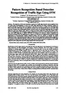
Model First off all, the name Hidden Markov Model (HMM) is chosen very badly. All dynamical systems being modeled have hidden state variables, so a Hidden Markov Model should be a model of a dynamical system that doesn’t make any assumptions except the Markov assumption. However, in literature, HMMs refer to models with the following extra assumptions: • The state space is discrete, ie. there’s a finite number of possible hidden states x. (eg. a mobile robot walking in a topological map: at kitchen door, in bed room, . . . ) • The measurement (observation) space is discrete. The difference between a Hidden Markov Model and a “normal” Markov Chain is the fact that the states of a normal Markov Chain are observable (and hence there is no estimation problem!). In other words, whereas for Markov Models, there’s a unique relationship between the state and the observation or measurement (no uncertainties), whilst for Hidden Markov Models the uncertainty between a certain measurement and the state it stems from is modeled by a probability density (see figure 3.2) Because of the discrete state and measurement spaces, each HMM can be represented as λ = (A, B, π) where eg. B ij = P (Z(i) = z j |x = xi ). The matrix A represents f (), B represents g() and π is used to determine in which state the HMM starts. The filter algorithms for HMMs are described in Section 4.2. Literature • “First paper”: [94] • Good introduction: [42], [61]: Here measurements are defined as inherently together with the transition between two states, whereas the normal approach considers them linked to a certain state. But the two approaches are entirely equivalent (this can be seen by redefining the state space (see eg. section 2.9.2 on p. 35 of [61]. See also http://www.univ-st-etienne.fr/eurise/pdupont/bib/hmm.html1 . 1 http://www.univ-st-etienne.fr/eurise/pdupont/bib/hmm.html
FIXM n ”bay
3.3. DISCRETE STATE VARIABLES, FINITE STATE MACHINE MODELING
25
Meas. B Meas. A
Meas. B Meas. A
state 1
state 2
Markov Model
state 1
Meas. C
state 2
Hidden Markov Model
Figure 3.2: Difference between a Markov Model and a Hidden Markov Model
Software • See the Speech Recognition HOWTO2 Extensions Standard HMMs are not very powerful models and appropriate for very particular cases only, so some extensions have been made to be able to use them for more complex and thus realistic situations: • Variable Duration HMMs Standard HMMs consider the chance to stay in a particular state as a exponential function of time � P x(k) = xi x(k − l) = xi ∼ e−l
As this is for most systems very unrealistic, Variable Duration HMMs [70, 71] solve this problem by introducing an extra, parametric, pdf P (Dj = d) (ie. a pdf predicting how long one typically stays in state j) to model the duration in a certain state. These are very appropriate for speech recognition.
• Monte Carlo HMMs) Monte Carlo HMMs [115, 116], also referred to as Generalized HMMs (GHMMs), extend the standard HMMs toward continuous state and measurement spaces. Whereas eg. in a normal HMM transitions between states are modeled by a matrix A, a MCHMM uses a non-parametric pdf to model state transitions (like a(xk |xk−1 , uk−1 , f k−1 )). Due to the fact that they don’t make any assumptions about any of the parameters involved, nor on the nature of the pdfs, in my opinion, GHMM filters can be used to describe strong non-linear problems such as the localization of transport pallets with a laser scanner (Memory/time requirements??), if defined as a dynamical system.
2 http://www.kulnet.kuleuven.ac.be/LDP/HOWTO/Speech-Recognition-HOWTO/index.html
FIX
26
CHAPTER 3. SYSTEM MODELING
Part II
Algorithms
27
Chapter 4
State estimation algorithms Literature describes different filters that calculate Bel(x(k)) or Bel(X(k)) for specific system and measurement models. Some of these algorithms calculate the full Belief function, others only some of its characteristics (mean, covariance, . . . ). This chapter gives an overview of the basic recursive (i.e., Markov) filters, without claiming to give a complete enumeration of the existing filters. To be able to determine which filter is applicable to a certain problem, one should verify certain things: 1. Is X a continuous or a discrete variable? (Eqs/graph) 2. Do we represent the pdfs involved as parametric distributions or do we use sampling techniques to be able to sample non-parametric distributions? 3. Are we solving a position tracking problem or a global localisation problem (unimodal or multimodal distributions) ... This section uses the previously defined symbols (xk , z k , . . . ). The detailed algorithms in appendix however, are described with the in the literature most common symbols for each specific filter.
4.1 Grid based and Monte Carlo Markov Chains Model The only assumption Markov Chains make is the Markov assumption. Thus, they do not make assumptions on the nature of x, nor on the nature of the pdfs that are used. Filter Markov Chains for discrete state variables directly solve Equations (2.6)–(2.7) for all possible values of the state. For continuous state variables they use numerical techniques, such as Monte Carlo-methods (often abbreviated as MC, see chapter 8) in order to ”discretize” the state space1 . Another applied discretization technique is the use of a grid over the entire state space. The corresponding filters are called MC Markov Chains and Grid-based Markov Chains. The Grid-based filters sample the state space in a uniform way, whereas the MC filters apply a different kind of sampling, most often referred to as importance sampling (see chapter8 ⇒ from where the name “particle filters”). Monte Carlo (particle) filters are also often referred to as the Condensation algorithm (mainly in vision applications), Survival of the fittest, or bootstrap filters. The most general and maybe most clear term appears to be sequential Monte Carlo methods. Particle Filters
FIXME: zowel
FIXME: Nog o.a
FIXME: KG: het algoritme dat je kan w zijn, zie o
• The basics: The SIS filter [39, 38] • To avoid the degeneracy of the sample weights: The SIR filter [100, 38, 52] • Smoothing the particles posterior distribution by a Markov Chain MC Move step [38] • Taking better proposal distributions then the system transition pdf [38]: Prior editing (niet goed), Rejection methods, Auxiliary particle filter [91] , Extended Kalman particle filter , Unscented Kalman particle filter 1 Note
that for continuous pdfs which can be parameterized, this discretization is not necessary, filters for these systems are described in section 4.4.
29
FIXME: u
FIXME: geb
L: do not understand volgende twee
: naar hoofdstuk MC
CHAPTER 4. STATE ESTIMATION ALGORITHMS
30 • any-time implementations The detailed algorithms are described in appendix D. Literature • first general paper?
• Good tutorials: [52] (Markov Localisation), [50] (= Monte Carlo version of [52]), [6]
4.2 Hidden Markov Model filters In literature, people do not write about HMM filters: They only speak about the different algorithms for HMMs. We chose to call them in this way to stress the similarities between the different techniques. Model
Finite state machines, see section 3.3.
Filter HMM filter algorithms typically calculate all state variables instead of just the last one: they solve (Eq. (2.4) instead of Eq. (2.1)). However, they do� not estimate the whole probability distribution of Bel(X(k)), they just give the � sequence of states X k = x0 , . . . , xk for which the joint a posteriori distribution Bel(X(k)) is maximal. The filter algorithm is often called the Viterbi algorithm (based on the Forward-backward algorithm). The version of both these algorithms for VDHMMs is fully described in appendix A. The algorithms for MCHMMs should be easy to derive from these algorithms. . . . Literature and software
See 3.3.2.
TODO • Verify if MCHMM filters sample the whole distribution or do they also just provide a state sequence that maximizes eq. 2.4. • Connection with MC Markov Chains ! Is there a difference? I think the only difference is the fact that MCHMM’s search a solution to the more general problem (eq. 2.4) and MC Markov Chains is just estimating the last hidden state xk (eq. 2.1) • Add HMM bookmarks?
4.3 Kalman filters Model Kalman filters are filters for equation models with continuous state variable X and with functions f () and g() that are linear in the state and uncertainties; i.e. eqs. (3.1)-(3.2) are: xk
= F k−1 xk−1 + f 0 k−1 (uk−1 , θ f ) + F 00 k−1 wk−1
zk
= Gk xk + g 0 k (sk , θ g ) + G00 k v k
F k−1 , F 00 k−1 , Gk and G00 k are matrices. Filter KFs estimate 2 characteristics of the pdf Bel(x(k)), namely the minimum-mean-squared-error (MMSE) estimate and covariance. Hence, their use is mainly restricted to unimodal distributions. A big advantage of KFs over the other filters is that KFs are computationally less expensive. The KF algorithm is described in appendix B. Literature • first general paper [63] • Good tutorial: [8]
4.4. EXACT NONLINEAR FILTERS Extensions
31
KFs are often applied to systems with non-linear system and/or measurement functions:
• Unimodal: the (Iterated) Extended KF [8] and Unscented KF [102] linearize the nonlinear system and measurement equations. • Multimodal: Gaussian sum filters [5] (often called multi hypothesis tracking in mobile robotics): for every mode (every Gaussian) an EKF is run. Remark 4.1 Note that the KF doesn’t assume Gaussian pdfs, but, for Gaussian pdfs the 2 characteristics estimated by the KF fully describe Bel(x(k)).
4.4 Exact Nonlinear Filters Model For some equation models with continuous state variables, pdf (2.1) can be represented by a fixed finite-dimensional sufficient statistic (the Kalman Filter is special case for Gaussian pdfs). [33] describes the systems for which the exponential family of probability distributions is a sufficient statistic, see appendix C. Filter The filter calculates the full (exponential) Bel(x(k)), the algorithm is given in appendix C. Literature
[33]
Extension:
approximations to other systems [33].
4.5 Rao-Blackwellised filtering algorithms
FIXME
In certain cases where some variables of the set of variables of the joint a posteriori distribution are independent of other ones, a mixed analytical/sample based algorithm can be used, combining the advantages of both worlds [82]. The FASTSlam algorithm [81, 79, 80] is a nice example of these.
4.6 Concluding Filter Grid-based Markov Chain MC Markov Chain HMM VDHMM MCHMM KF EKF, UKF Gaussian sum Daum
X C C D D C C C C C
P (X) n’importe n’importe n’importe n’importe n’importe unimodal unimodal multimodal exponential
Varia Computationally expensive Subdivide (rejection, metropolis, . . . ) x = max P(X), eq. (2.4) x = max P(X), eq. (2.4) ????? f () and g() linear f () and g() not too unlinear f () and g() not too unlinear rare cases (appendix C)
32
CHAPTER 4. STATE ESTIMATION ALGORITHMS
Chapter 5
Parameter learning All Bayesian approaches use explicit system and measurement models of their environment. In some cases, the construction of good enough models to approximate the system state in a satisfying manner is impossible. Speech is an ideal example: every person has a different way of pronouncing different letters (such as in “Bruhhe”). The system and measurement models and the characteristics of their uncertainties are written in function of inaccurately known parameters, collected in the vectors θ f , respectively θ g . In a Bayesian context, estimation of those parameters would typically be done by maintaining a pdf over the space of all possible parameter values. The inaccurately known parameters θ f and θ g have to be estimated online, next to the estimation of the state variables. This is often called parameter learning (mapping in mobile robotics). The initial state estimation problem of Chapters 2–4 is augmented to a concurrent-state-estimation-andparameter-learning problem (“simultaneous localization and mapping (SLAM)” or “concurrent mapping and localization (CML)” in mobile robotics�terminology). To simplify the notation of the following equations, θ f and θ g are collected into � θf one parameter vector θ = . Remark that any estimate for this vector is valid for all time steps (parameters are constant θg in time . . . ). If the parameter vector θ comes from a limited discrete distribution, the problem can be solved by multiple model filtering (Section 5.3). However if the parameter vector θ does not come from a limited discrete distribution, —IMHO— the only ‘right’ way to handle the concurrent-state-estimation-and-parameter-learning problem is to augment the state vector with the inaccurately known parameters (Section 5.1). However if a lot of parameters are inaccurately known, up till now, the resulting state estimation problem is only succesfully solved with Kalman Filters (on problems that obey the corresponding assumptions). In other cases, the computational less expensive Expectation-Maximization algorithm (EM, Section 5.2) is often used as an alternative. The EM algorithm subdivides the problem in two steps: one state estimation step and one parameter learning step. The algorithm is a method for searching a local maximum of the pdf P (z k |θ) (consider this pdf as a function of θ). Parameter learning is also sometimes called model building. IMHO, this can be use to construct models in which some parameters are not accurately known, or in situations where is it very difficult to construct an off-line, analytical model. I’ll try to clarify this with the example of the localization of a transport pallet with a mobile robot, equipped with a laser scanner. It is very difficult (but not impossible) to create off-line a fully correct measurement distribution (ie. taking sensor uncertainty/characteristics into account), for a state x = [x, y, θ]T : � P z k x(k) = [xk yk θk ]T , sk , θ g , g k
Figure 5.1 illustrates this. Experiments should point out whether off-line construction of this likelihood function is faster than learning.
5.1 Augmenting the state space In order to solve the concurrent-state-estimation-and-parameter-learning problem, the state vector can be augmented with � � x . These parameters are then estimated within the state estimation problem. the model parameters x ←− θ Filters Augmenting the state space is possible for all state estimators, as long as the new state, system and measurement model still obey the estimator’s assumptions. In the specific case of a Kalman Filter, estimating state and parameters simultaneously by augmenting the state vector is called “Joint Kalman Filtering”, [122]. 33
FIXME: KG lo measured fea inaccurately k
FIXME: KG without taking the best way to
CHAPTER 5. PARAMETER LEARNING
34 � $ % �
$ %
$ %
$ � % �
$ %
#
"
$ %
#
!
!
!
"
$ %
$ %
$ %
!
!
!
$ %
$ %
$ %
!
!
!
$ %
$ %
$ %
�
!
!
!
$ %
$ %
$ %
� � � �
� �
� �
!
!
!
$ %
$ %
$ %
� � � �
� �
� �
!
!
!
$ %
$ %
$ %
� �
� �
� �
� �
� �
� �
!
!
!
$ %
$ %
$ %
� �
� �
� �
� �
� �
� �
!
!
!
$ %
$ %
$ %
� �
� �
� �
� �
!
!
$ %
$ %
$ %
� �
� �
� �
� �
� �
!
!
!
$ %
$ %
$ %
� �
� �
� �
� �
� �
� �
� �
� �
!
!
!
$ %
$ %
$ %
� �
� �
� �
� �
� �
�
�
� �
� �
� �
�
�
� �
� �
� �
!
$ % � � � �
� �
� �
� �
� �
� �
� �
!
!
!
$ % � �
� �
$ % � � � �
$ % � � � �
� �
� �
� �
� �
� �
� �
!
!
!
$ % � �
� �
$ % � � � �
$ % � � � �
� �
� �
� �
� �
� �
� �
!
!
!
$ % � �
� �
$ % � � � �
$ % � � � �
� �
� �
� �
� �
� �
� �
!
!
!
$ % � �
� �
$ % � � � �
$ % � � � �
� �
� �
� �
� �
� �
� �
!
!
!
$ % � �
� �
$ % � � � �
$ % � � � �
� �
� �
� �
� �
� �
� �
!
!
!
$ % � �
� �
$ % � � � �
$ % � � � �
� �
�
� �
!
$ % � �
� �
$ % � � � �
$ % � � � �
�
� �
�
� �
� �
� �
� �
� �
� �
� �
� �
� �
� �
� �
� �
!
!
!
$ % � �
� �
$ % � � � �
$ % � � � �
� �
� �
� �
� �
� �
� �
� �
!
� �
� �
!
!
!
$ % � �
� �
$ % � � � �
$ % � � � �
� �
� �
� �
� �
�
� �
�
� �
� �
!
� �
�
� �
!
$ % � � � �
� �
�
� �
� �
!
$ % � �
� �
� �
�
� �
� �
!
� �
� �
� �
� �
!
!
!
$ % � �
� �
$ % � � � �
$ % � � � �
� �
� �
� �
� �
� �
� �
� �
�
!
!
!
$ % � �
� �
$ % � � � �
$ % � � � �
� �
� �
� �
� �
� �
� �
!
!
!
$ % � �
� �
$ % � � � �
$ % � � � �
� �
� �
� �
� �
� �
� �
!
!
!
$ % � �
� �
$ % � � � �
$ % � � � �
� �
� �
� �
� �
� �
� �
!
!
!
$ % � �
� �
$ % � � � �
$ % � � � �
� �
� �
� �
� �
� �
� �
!
!
!
$ % � �
� �
$ % � � � �
$ % � � � �
� �
� �
� �
� �
� �
� �
!
!
!
$ % � �
� �
$ % � � � �
$ % � � � �
� �
� �
� �
� �
!
!
$ % � �
� �
$ % � � � �
$ % � � � �
� �
� �
� �
!
!
$ % � �
� �
$ % � � � �
$ % � � � �
� �
� �
� �
� �
!
!
$ % � � � �
$ % � � � �
� �
� �
� �
� �
� �
� �
� �
� �
� �
� �
!
$ % � �
� �
� �
� �
� �
� �
!
� �
� �
� �
� �
!
� �
� �
� �
� �
!
!
!
$ % � �
� �
$ % � � � �
$ % � � � �
� �
� �
� �
� �
Figure 5.1: Illustration of the complexity `of the ˛ measurement model ´of a transport pallet. The figure shows two pallets in a different position. Imagine how to set up the pdf P z k ˛x(k) = [xk yk θk ]T , sk . The pallet on the above right side doesn’t cause much trouble. However, the location of the pallet on the left side below causes more trouble. First for every possible location, one has to search the intersection of the laserbeam (with orientation sk ) and the pallet. This is already quite complicated. But, most likely, there will also be uncertainty on sk , such that some particular laserbeams (such as the dash-dotted one in the figure) can actually reflect on either one “poot” of the pallet or the other one (further behind) all location and we would create a kind of multi-modal gaussian with 2 peaks. So for some cases, the measurement function becomes really complex
5.2 EM algorithm As discribed in the introduction, augmenting the state space with many parameters often leads to computational difficulties, if a KF is not a good model for the (non-linear) system. The EM algorithm is an often used technique for these cases. However, is it not a Bayesian technique for parameter estimation and (thus :-) not an ideal solution for parameter estimation! The EM algorithm consists of two steps: 1. the E-step (or state estimation step) the pdf over all previous states X(k) is estimated based on the current best parameter estimate θ k−1 : � � P X(k) Z k , U k−1 , S k , θ k−1 , F k−1 , Gk , P (X(0)) This problem is a state estimation problem as described in the previous chapter. Remark 5.1 Note that this is a Batch method with a not-constant evaluation time!! For every new map, we recalculate the whole state sequence! This is a batch method and not very well suited for real-time applications
5.2. EM ALGORITHM
35
With this pdf, the expected value of the logarithm of the complete-data likelihood function P X(k), Z k U k−1 , S k , θ, F k−1 , Gk , P is evaluated:
Q(θ, θ k−1 ) = �i (5.1) �� E log P X(k), Z k U k−1 , θ, . . . , P (X(0)) | P X k Z k , U k−1 , θ k−1 , . . . , P (X(0)) h �i � E f (X k ) P X k |Z k , U k−1 , S k , θ k−1 , F k−1 , Gk , P (X(0)) means that the expectation of the function f (X k ) � is sought when X k is a random variable distributed according to the a posteriori pdf P X(k) Z k , U k−1 , S k , θ k−1 , F k−1 , Gk , P (X Eg. for a continuous state variable this means: Z �� Q(θ, θ k−1 ) = log P X(k), Z k U k−1 , S k , θ, F k−1 , Gk , P (X(0))) � � P X(k) Z k , U k−1 , S k , θ k−1 , F k−1 , Gk , P (X(0)) dX(k). �
h
NOTE: θ k−1 is not a parameter of this function, but it’s value does influence the function! The evaluation of this integral can be done with eg. Monte Carlo methods. If we are using a particle filter (see chapter D), expression 5.1 reduces to N X �� k−1 log P X i (k), Z k U k−1 , S k , θ, F k−1 , Gk , P (X(0)) Q(θ, θ )= i=1
where X i (k) denotes the i-th sample of the complete data-likelihood pdf (which we don’t know). Application of Bayes’ rule and the Markov assumption on the previous expression gives Q(θ, θ k−1 ) = ≈ =
N X i=1
N X i=1
� �� � log P Z k X i (k), U k−1 , S k , θ, F k−1 , Gk , P (X(0)) P X i (k) U k−1 , S k , θ, F k−1 , Gk , P (X(0))
� �� � log P Z k X i (k), S k , θ g , Gk P X i (k) U k−1 , θ f , F k−1 , P (X(0))
The left hand term of the log product is the measurement equation, with θ considered as a parameter and specific values for the state and the measurement. The right hand side of the equation is the result of a dead-reckoning exercice, with θ considered as a parameter. However we don’t know this PDF as a function of θ :-(. 2. the M-step (or parameter learning step) a new estimate θ k is calculated for which the the (incomplete-data) likelihood function increases: � � � p Z k U k−1 , S k , θ k , F k−1 , Gk , P (X(0)) > p Z k U k−1 , S k , θ k−1 , F k−1 , Gk , P (X(0)) .
FIXME: KG this!! IMHO linear
(5.2)
This estimate θ k is calculated as the θ which maximizes the expected value of the logarithm of the complete-data likelihood function: θ k = argmax Q(θ, θ k−1 ); (5.3) or at least increases it (this version of the EM algorithm is called the Generalized EM algorithm (GEM)): Q(θ k , θ k−1 ) > Q(θ k−1 , θ k−1 )
(5.4)
Appendix E proves that a solution to (5.3) or (5.4) satisfies (5.2). Remark 5.2 Note that in this section, the superscript k in θ k. refers to the estimate for θ . in the kth iteration. This estimate is valid for all timesteps because θ . is static.
Remark 5.3 Sometimes the E-step calculates p(X(k), Z k |U k−1 , S k , θ k−1 , F k−1 , Gk , P (X(0))) instead of p(X(k)|Z k , U k−1 , S k , θ k Both differ only in a factor p(Z k |U k−1 , S k , θ k−1 , F k−1 , Gk , P (X(0))). This factor is independent of the variable θ and hence does not affect the M-step of the algorithm. Remark 5.4 Note that the EM algorithm calculates at each time step the full pdf over X, but it only calculates one θ which maximizes or increases Q(θ, θ k−1 ).
d Grid-based HMMs?
CHAPTER 5. PARAMETER LEARNING
36 Filters
1. All HMM filters allow the use of EM. The algorithm is most often known as the Baum-Welch algorithm (appendix A gives the concrete formulas for the VDHMM; for a derivation starting from the general EM algorithm, see [61]). In the case of MCHMMs , where pdf’s are non parametric, the danger for overfitting is real and regularization is absolutely necessary. Typically cross-validation techniques are used to avoid this (shrinkage and annealing).
Work this further out
Relate this to Pattern Recognition
2. Dual Kalman Filtering [122]. The algorithm is described in appendix B.
5.3 Multiple Model Filtering When the parameters are discrete and there is only a limited number of possible parameters, the concurrent-state-estimationand-parameter-learning problem can be solved by a Multiple Model Filter. A Multiple Model Filter considers a fixed number of models, one for each possible value of the parameters. So, in each filter, the parameters are different but known (the different models can also have different structure, different parameterization). For each of the models a separate filter is run. Two kinds of Multiple Model Filter exist: 1. Model detection (model selection, model switching, multiple model, multiple model hypothesis testing, . . . ) filters try to identify the “correct” model, the other models are neglected. 2. Model fusion (interacting multiple model, . . . ) filters calculate a weighted state estimate between the models. Filters Multiple Model Filtering is possible with all filtering algorithms, however, in practice, it is almost only applied for Kalman Filters, because most other filters are computationally too complex to run several of them in parallel.
Chapter 6
Decision Making In the previous chapters, we learned how to process measurements in order to obtain estimates for states and parameters. When we have a closer look at the system’s proces and measurement functions () and (), we see that the system’s states and measurements are influenced by the input to the system. This input can be in the proces function (e.g. an acceleration input), or in the measurement function (e.g. a parameter of the sensor). The previous chapters assumed that these inputs were given and known. This chapter is about planning (decision making), about the choice of the inputs (control signals, actions). Indeed, a different input can lead to more accurate estimates of the states and/or parameters. So, we want to optimize the input in some way to get “the best possible estimates” (optimal experiment design) and in the mean while perform the task “as good as possible”, i.e. to perform active sensing. An example is mobile robot navigation in a known map. The robot is unsure about its exact position in the map and needs to determine the action that determines best where it is in the map. Some people make the distinction between active localization and active sensing. The former then refers to robot motion decisions, the latter to sensing decisions (e.g. when a robot is allowed to fire only one sensor at a time). Section 6.1 formulates the active sensing problem. The performance criteria Uj which measure the gain in accuracy of the estimates are explained in section 6.2. Section 6.3 describes possible ways to model the input trajectories. Section 6.4 discusses some optimization procedures. Section 6.8 discusses model-free learning, i.e. when there is no model (or not yet an exact model) of the system available.
6.1 Problem formulation We consider a dynamic system described by the state space model xk+1 = f (xk , uk , η k )
(6.1)
z k+1 = h(xk+1 , sk+1 , ξ k+1 )
(6.2)
where x is the system state vector, f and h nonlinear system and measurement functions, z is the measurement vector, η and ξ are respectively system and measurement noises. u stands for the input vector of the state function, s stands for a sensor parameter vector as input of the measurement function (an example is the focal length of a camera). The subscripts k and k + 1 stand for the time step. The system’s states and measurements �are influenced � by the inputs u and s. Further, we make no distinction and denote both inputs to the system with ak = uk sk+1 (actions). Conventional systems consisting only of control and estimation components assume that these inputs are given and known. Intelligent systems should be able to perform active sensing. A first thing we have to do is choose a multiobjective performance � criterium, (often � called value function or return function), that determines when the result of a sequence of actions π 0 = a0 . . . aN −1 1 (also called policy) is considered to be “better” than the result of another policy: X X βl Cl (...)} (6.3) αj Uj (...) + V ∗ = min V () = min{ π0
π0
j
l
This criterion (or cost function) is a weighted sum of expected costs: The optimal policy π 0 is the one that minimizes this function. The cost function consists of 1 The
index 0 denotes that π contains all actions starting from time 0
37
FIXME: re Markov Models - Hidden Mark
: KG: Look for better formulation
: Maybe add index to merate the constraints
CHAPTER 6. DECISION MAKING
38
1. j terms αj Uj (...) characterizing the minimization of expected uncertainties Uj (...) (maximization of expected information extraction) and 2. l terms βl Cl (...) denoting other expected costs and utilities Cl (...), such as time, energy, distances to obstacles, distance to the goal. The weighting coefficients αj and βl are chosen by the designer and reflect his personal preferences . A reward/cost can be associated both with an action a as with the arrival in a certain state x. If both the goal configuration and the intermediate time evolution of the system are important with respect to the calulation of the cost function, the terms Uj (...) and Cl (...) are themselves a function of the Uj,k ()... and Cl,k (...) at different time steps k. If the probability distribution over the state at the goal configuration p(xN |x0 , π 0 ) fully determines the rewards, these components are reduced into their last terms and V is calculated by using Uj,N and Cl,N only. V is to be minimized with respect to the sequence of actions under certain constraints c(x0 , . . . , xN , π 0 ) ≤ cmax .
(6.4)
The thresholds cmax express for instance maximal allowed velocities and acceleration, maximal steering angle, minimum distance to obstacles, etc. The problem could be a finite-horizon (over a fixed, finite number of time steps) or an infinite-horizon problem (N = ∞). For infinite horizon problems: [15, 93] • the problem can be posed as one in which we wish to maximize expected average reward per time step, or expected total reward; • in some cases, the problem itself is structured so that reward is bounded (e.g. goal reward, all actions: cost), once in goal state: stay at no cost; • sometimes, one uses a a discount factor (”discounting”): rewards in the far future have less weight than rewards in the near future.
6.2 Performance criteria for accuracy of the estimates The terms Uj,k (...) represent (i) the expected uncertainty of the system about its state; or (ii) this uncertainty compared to the accuracy needed for the task completion. In a Bayesian framework, the characterization of the uncertainty of the estimate is based on a scalar loss function of its probability density function. Since no scalar function can capture all aspects of a pdf, no function suits the needs of every experiment. Common used functions are based on a loss function of the covariance matrix of the pdf or on the entropy of the full pdf. Active sensing is looking for the actions which minimize • the posterior pdf: p = ... in the following formulas • the “distance” between the prior and the posterior pdf: p1 = ... and p2 = ... in the following formulas • the “distance” between the posterior and the goal pdf: p1 = ... and p2 = ... in the following formulas • the posterior covariance matrix (P = P post in the following functions) • the inverse of the Fisher information matrix I [48] which describes the posterior covariance matrix of an efficient estimator (P = I −1 in the following functions). Appendix H gives more details on the Fisher info matrix and the Cramer Rao. • loss function based on the covariance matrix: The covariance matrix P of the estimated pdf of state x is a measure of the uncertainty of the estimate. Since no scalar function can capture all aspects of a matrix, no loss function suits the needs of every experiment. Minimization of a scalar loss function of the posterior covariance matrix is extensively described in the literature of optimal experiment design [47, 92] where several scalar loss functions have been proposed: – D-optimal design: minimizes det(P ) or log(det(P ))). The minimum is invariant to any transformation of the variables x with a nonsingular Jacobian (e.g. scaling). Unfortunately, this measure does not allow to verify task completion.
6.2. PERFORMANCE CRITERIA FOR ACCURACY OF THE ESTIMATES
39
– A-optimal design: minimizes the trace tr(P ). Unlike D-optimal design, A-optimal design does not have the invariance property. The measure does not even make sense physically if the target states have inconsistent units. On the other hand, this measure allows to verify task completion (pessimistic). – L-optimal design: minimizes the weighted trace tr(W P ). A proper choice of the matrix W can render the L-optimal design criterium invariant to transformations of the variables x with a nonsingular Jacobian: W has units and is also transformed accordingly. A special case of L-optimal design is the tolerance-weighted L-optimal design [34, 53], which proposes a natural choice of W depending on the desired standard deviations / tolerances at task completion. The value of this scalar function has a direct relation to the task completion. – E-optimal design: minimizes the maximum eigenvalue λmax (P ). Like A-optimal design, this is not invariant to transformations of x, nor the measure makes sense physically if the target states have inconsistent units; but the measure allows to verify task completion (pessimistic). • loss function based on the entropy: Entropy is a measure of uncertainty represented by the probability distribution. This measure has more information about the pdf than only the covariance matrix, which is important for multimodal distributions, consisting of several small peaks. Entropy is defined as: H(x) = E[− log p(x)]. For a discrete distribution (p(x = x1 ) = p1 , . . . , p(x = xn ) = pn ) this is: H(x) = − for continuous distributions: H(x) = −
Z
n X
pi log pi
(6.5)
i=1
∞
p(x) log p(x)dx
(6.6)
−∞
Appendix G describes the concept of entropy in more detail. Some entropy based performance criteria are: – the entropy of the distribution: H(x) = E[− log p(x)]. !! not invariant to transformation of x !!?? – the change in entropy between two distributions p1 (x) and p2 (x): H2 (x) − H1 (x) = E[− log p2 (x)] − E[− log p1 (x)]
(6.7)
If we make the change between the entropy of the prior distribution p(x|Zk ) and the conditional distribution p(x|Zk+1 ); this measure corresponds to the mutual information (see appendix G.5). Note that the entropy of the conditional distribution p(x|Zk+1 ) is not the equal to the entropy of the posterior distribution p(x|Zk+1 ) (see appendix G.3)! – the Kullback-Leibler distance or relative entropy is a measure for the goodness of fit or closeness of two distributions: p2 (x) ]; (6.8) D(p2 (x)||p1 (x)) = E[log p1 (x) where the expected value E[.] is calculated with respect to p2 (x). For discrete distributions: n X
D(p2 (x)||p1 (x)) =
i=1
p2,i (x) log p2,i (x) −
n X
p2 (x) log p2 (x)dx −
Z
p2,i (x) log p1,i (x)
(6.9)
i=1
For continuous distributions: D(p2 (x)||p1 (x)) =
Z
∞
−∞
∞
p2 (x) log p1 (x)dx
(6.10)
−∞
Note that the change in entropy and the relative entropy are different measures. The change in entropy only quantifies how much the form of the pdfs changes; the relative entropy also incorporates a measure of how much the pdf moves: if p1 (x) and p2 (x) are the same pdf, but translated to another mean value, the change in entropy is zero, while the relative entropy is not. The question of which measure is best to use for active sensing is not an issue as the decision making is based on the expectations of the change in entropy or relative entropy, which are equal. Remark: Minimizing the covariance matrix is often a more appropriate active sensing criterion than minimizing an entropy function of the full pdf. This is the case when we want to estimate our state unambiguously, i.e. when we want to use one value for the state estimate, and reduce the uncertainty of this estimate maximally. The entropy will not always be a good measure because for multimodal distributions (ambiguity in the estimate) the entropy can be very small while the uncertainty on any possible state estimate is still large. With the expected value of the distribution as estimate, the covariance matrix indicates how uncertain this estimate is.
CHAPTER 6. DECISION MAKING
40
6.3 Trajectory generation The description of the possible sequence of actions ak can be done in different ways. This has a mayor impact on the optimization problem to solve afterwards (section 6.4). • The evolution of ak can be restricted to trajectory, described by a reference trajectory and a parametrized deviation of this trajectory. In this way, the optimization problem is reduced to a finite-dimensional, parameterized optimization problem. Examples are the parameterization of the deviation as finite sine/cosine series. • A more general way to describe the trajectory is a sequence of freely to choose actions, that are not restricted to a certain form of trajectory. The optimization of such a sequence of decisions over time and under uncertainty is called dynamic programming. At execution time, the state of the system is known at any time step. If there is no measurement uncertainty at execution time, the problem is a Markov Decision Proces (MDP) for which the optimal policy can calculated before the task execution for each possible state at every possible time step in the execution (a policy that maximizes the total future expected reward). If the measurements are noisy, the problem is a Partially Observable Markov Decision Proces (POMDP). This means that at execution time the state of the system is not known, only a probability distribution over the states can be calculated. For this case, we need an optimal policy for every possible probability distribution at every possible time step. No need to say that this complicates the solution a lot.
6.4 Optimization algorithms 6.5 If the sequence of actions is restricted to a parameterized trajectory E.g. dynamical robot identification [22, 113]. The optimization can have different forms, depending on the function to optimize and the constraints: linear programming, constrained nonlinear least squares methods, convex optimization, etc. The references in this section are just examples, and not necessarily to the earliest nor the most famous works. A. Local optimum = global optimum: • Linear programming [90]: linear objective function and constraints, which may include both equalities and inequalities. Two basic methods: – simplex method: each step is to move from one vertex of the feasible set to an adjacent one with a lower value of the objective function. – the interior-point methods, e.g. the primal-dual interior point methods: they require all iterates to satisfy the inequality constraints in the problem strictly. • Convex programming (e.g. semidefinite programming) [21]: convex (or linear) objective function and constraints, which may include both equalities and inequalities. B.Nonlinear-nonconvex problems: 1. Local optimization methods [90]: • Unconstrained optimization – Line search methods: starts by fixing the direction (Steepest descent direction, any-descent direction, Newton direction, Quasi-Newton direction, conjugate gradient direction), then identifies an approximate step distance (with lower function value). – Trust region methods: first chooses a maximum distance, then approximate the objectve function in that region (linear or quadratic) and then seeks a direction and step length (Steepest descent direction and Cauchy point, Newton direction, Quasi-Newton direction, conjugate gradient direction). • Constrained optimization: e.g. reduced-gradient methods, sequential linear and quadratic programming methods and methods based on Lagrangians, penalty functions, augmented Lagrangians. 2. Global optimization methods: The Global Optimization website by Arnold Neumaier2 gives a nice overview of various optimization problems and solutions. 2 http://solon.cma.univie.ac.at/∼neum/glopt.html
6.6. MARKOV DECISION PROCESSES
41
• Deterministic – Branch and Bound methods: Mixed Integer Programming, Constraint Satisfaction Techniques, DC-Methods, Interval Methods, Stochastic Methods – Homotopy – Relaxation • Stochastic – Evolutionary computation: genetic algorithms (not good), evolution strategies (good), evolutionary programming, etc – Adaptive Stochastic Methods: (good) – Simulated Annealing (not good) • Hybrids: ad-hoc or involved combinations of the above – Clustering – 2-phase
6.6 Markov Decision Processes Original books and papers that describe MDPs: [10, 11, 58] Modern works on MDPs: [14, 15, 73, 93] ** What is MDP ** If the sequence of actions is not restricted to a parametrized trajectory, then the optimization problem has a different structure: (PO)MDP. This could be a finite-horizon, i.e. over a fixed finite number of time steps (N is finite), or an infinite-horizon problem (N = ∞). For every state it is rather straightforward to know the immediate reward being associated to every action (1 step policy). The goal however is to find the policy that maximizes the reward over a long term (N steps). ∗
The optimal policy is π ∗0 , if V π0 (x0 ) ≥ V π0 (x0 ), ∀π 0 , x0 . For large problems (many states, many possible actions, large N,...) it is computationally not tractable to calculate all value functions V π0 (x0 ) for all policies π 0 . Some techniques have been developed that exploit the fact that an infinite-horizon problem will have an optimal stationary policy, a characteristic not shared by their finite horizon counterparts. Although MDPs can be both continuous or discrete systems, we will focus on the discrete (discrete actions / states) stochastic version of the optimal control problem. Extensions to real-valued states and observations can be made. There are two basic strategies for approximating the solution to a continuous MDP [101]: • discrete approximations: grid, Monte Carlo [114], . . . • smooth approximations: treat the value function V and/or decision rules π as smooth, flexible functions of the state x and a finite-dimensional parameter vector θ Discrete MDP problems can be solved exactly, whereas the solutions to continuous MDPs can generally only be approximated. Approximate solution methods may also be attractive for solving discrete MDPs with a large number of possible states or actions. Standard methods to solve: Value iteration: optimal solution for finite and infinite horizon problems ** For every state xk−1 it is rather straightforward to know the immediate reward being associated to an action ak−1 (1 step policy): R(xk−1 , ak−1 ). The goal however is to find the policy π0∗ that maximizes the (expected) reward over the long term (N steps). The future reward is function of the starting state/pdf xk−1 and the executed policy πk = (ak−1 , . . . , aN −1 ) at time k − 1: X {P (xk |xk−1 , ak−1 )V πk (xk )} (6.11) V πk−1 (xk−1 ) = R(xk−1 , ak−1 ) + γ xk
This is a backward recursive calculation. 0 ≤ γ ≤ 1
CHAPTER 6. DECISION MAKING
42
ak−1
� Z = arg max R(xk−1 , a) + γ a
xk
V (xk )p(xk |xk−1 , a)dxk
�
(6.12)
bellmans equation: Vk−1
� Z = max R(xk−1 , a) + γ a
xk
"
ak−1 = arg max R(xk−1 , a) + γ a
"
Vk−1 = max R(xk−1 , a) + γ a
(6.13)
#
V (xk )p(xk |xk−1 , a)
(6.14)
#
(6.15)
V (xk )p(xk |xk−1 , a)dxk X xk
bellmans equation:
�
X xk
V (xk )p(xk |xk−1 , a)
** We exploit the sequential structure of the problem: the optimization problem minimizes (or maximizes) V , written as a succession of sequential problems to be solved with only 1 of the N variables ai . This way of optimizing is called dynamic programming (DP)3 and is introduced by Richard Bellman [10] with his Principle of Optimality, also known as Bellman’s principle: ∗ An optimal policy πk−1 has the property that whatever the initial state xk−1 and the initial decision ak−1 are, the remaining ∗ decisions πk must constitute an optimal policy with regard to the state xk resulting from the first decision (xk−1 , ak−1 ). The intuitive justification of this principle is simple: if πk∗ were not optimal as stated, we would be able to maximize the reward further by switching to an optimal policy for the subproblem once we reach xk . This makes a recursive calculation of the optimal policy possible: finding an optimal policy for the system when N − i time steps remain, can be optained by using the optimal policy for the next time step (i.e. when N − i − 1 steps remain); and is expressed in the Bellman equation (aka functional equation): for discrete state space: ( ) o Xn ∗ ∗ P (xk |xk−1 , ak−1 )V πk (xk ) V πk−1 (xk−1 ) = max E R(xk−1 , ak−1 ) + γ (6.16) ak−1
xk
for continuous state space: V
∗ πk−1
� Z (xk−1 ) = max E R(xk−1 , ak−1 ) + γ ak−1
xk
P (xk |xk−1 , ak−1 )V
∗ πk
(xk )dxk
�
(6.17)
MDP: E OVER PROCESRUIS. The solution of the MDP problem with dynamic programming is called value iteration [10]. The algorithm starts with the ∗ ∗ ∗ value function V πN (xN ) = R(xN ) and computes the value function for 1 more time step (V πk−1 ) based on (V πk ) using ∗ Bellman’s equation (6.16) untill V π0 (x0 ) is obtained. This method works for both finite and infinite MDPs. For infinite horizon problems Bellman’s equation is iterated till convergence. Note that the algorithm may be quite time consuming, since the minimization in the DP must be carried out ∀xk , ∀ak . curse of dimensionality. policy iteration: optimal solution for infinite horizon problems Policy iteration is an iterative technique similar to dynamic programming, introduced by Howard [58]. The algorithm starts with any policy (for all states), called π 0 . Following iterations are performed: i
1. evaluate the value function V π (x) for the current policy with an (iterative) policy evaluation algorithm 2. improve the policies with a policy improvement algorithm: ∀x, find the action a∗ that maximizes o Xn i Q(a, x) = R(x, a) + γ P (x0 |a, x)V π (x0 ) x0
i
if Q(a, x) > V π (x0 ), let π i+1 (x) = a∗ else keep π i+1 (x) = π i (x). π i+1 (x) = π i (x), ∀x. 3 dynamic programming: optimization in a dynamic context; “dynamic” time plays a significant role
(6.18)
6.6. MARKOV DECISION PROCESSES
43
modified policy algorithm: optimal solution for infinite horizon problems The modified policy algorithm [93] is a combination of the policy iteration and value iteration methods. Like policy iteration, the algorithm contains a policy improvement step and a policy evaluation step. However, the evaluation step is not done exactly. The key insight is that one need not to evaluate a policy exactly in order to improve it. The policy evaluation step is solved approximately by executing a limited number of value iterations. Like the value iteration , it is an iterative method starting with a value V πN and iterates till convergence. linear programming: optimal solution for infinite horizonproblems horizon MDP problem: X V (x) minV
[93, 36, 105] value function for a discrete infinite (6.19)
x
s.t.V (x) ≥ R(x, a) + γ
X x0
{V (x0 )p(x0 |x, a)}
(6.20)
a and x over all possible actions and states. Linear programs are solved with (1) the Simplex Method or (2) the Interior Point Method [90]. Linear programming is generally less efficient than the previously mentioned techniques because it does not exploit the dynamic programming structure of the problem. However, [118] showed that sometimes it is a good solution. state based search methods (AI planning): optimal solution [19] The solution here is to build suitable structures (e.g. a graph4 , a set of clauses,...) and then search them. The heuristici search can be in state space [18] or in belief space [17] These methods explicitly search the state or belief space with a heuristic that estimates the cost from this state or belief to the goal state or belief. Several planning heuristics have been proposed. The simplest one is a greedy search where we select the best node for expansion and forget about the rest. Real time dynamic programming [9] is a combination of value iteration for dynamic programming and a greedy heuristic search. Real time dynamic programming is guaranteed to yield optimal solutions for a large class of finite-state MDPs. Dynamic programming algorithms generally require explicit enumeration of the state space at each iteration, while search techniques enumerate only reachable states. However, at sufficient depth in the search tree, individual states can be enumerated multiple times, whereas they are considered only once per stage in dynamic programming. Approximations without enumeration of the state: approx, finite and infinite hor The previously mentioned methods are optimal algorithms to solve MDPs. Unfortunately, we can only find exact solutions for small MDPs because these methods produce optimal policies in explicit form (i.e. tabular manner that enumerates the state space). For larger MDPs, we must resort to approximate solutions [19], [101]. To this point our discussion of MDPs has used an explicit or extensional representation for the set of states (and actions) in which states are enumerated directly. We identify three ways in which structural regularities can be recognized, represented, and exploited computationally to solve MDPs effectively without enumeration of the state space • simplyfying assumptions such as observability, no process uncertainty, goal satisfaction, time-separable value functions, . . . can make the problem computationally easier to solve. In the AI literature, many different models are presented which can in most cases be viewed as special cases of MDPs and POMDPs. • in many cases it is advantageous to compact the states, actions and rewards representation (factored representation). Also the components of a problem’s solution, i.e. the policy and optimal value function, are also candidates for compact structured representation. Following algorithms use these factored representations to avoid iterating explicitly over the entire set of states and actions: – aggregation and abstraction techniques: these techniques allow the explicit or implicit grouping of states that are indistinguishable with respect to certain characteristics (e.g. the value function or the optimal action choice). – decomposition techniques: (i) techniques relying on reachability and serial decomposition: an MDP is broken into various pieces, each of which is solved independently; the solutions are then pieced together or used to guide the search for a global solution. The reachability analysis restricts the attention to “relevant ” regions of state space. and (ii) parallel decomposition in which an MDP is broken into a set of sub-MDPs that are “run in parallel”. Specifically, at each stage of the (global) decision process, the state of each subprocess is affected. while most of these methods provide approximate solutions, some of them offer optimality guarantees in general, and most can provide optimal solutions under suitable assumptions. 4 One way to formulate the problem as a graph search is to make each node of the graph correspond to a state. The inital and goal states can then be identified, and the search can proceed either forward or backward through the graph, or in both directions simultaneously.
CHAPTER 6. DECISION MAKING
44
Limited lookahead: approximate solution for finite and infinite horizon problems. The limited lookahead is to truncate the time horizon and use at each stage a decision based on a lookahead of a small number of stages. The simplest possibility is to use a one-step lookahead policy.
6.7 Partially Observable Markov Decision Processes ** for discrete state space: V
∗ πk−1
(xk−1 ) = max E ak−1
) o Xn ∗ R(xk−1 , ak−1 ) + γ P (xk |xk−1 , ak−1 )V πk (xk )
(
(6.21)
xk
MDP: E OVER PROCESRUIS; POMDP E OVER STATE, PROCESRUIS, MEETRUIS for continuous state space: � � Z ∗ ∗ πk πk−1 (6.22) P (xk |xk−1 , ak−1 )V (xk )dxk V (xk−1 ) = max E R(xk−1 , ak−1 ) + γ ak−1
xk
Unfortunately, in many practical cases and analytical solution is not possible, and one has to resort to numerical execution of the DP algorithm. This may be quite time consuming, since the minimization in the DP must be carried out ∀xk , ∀ak , (∀zk : P OM DP ). This means that the state space must be discretized in some way (if it is not already a finite set). curse of dimensionality ** What is POMDP ** Original books/papers on POMDP: [41], [7] Survey algorithms: Lovejoy [74] E.g. for mobile robotics: [99, 24, 65, 51, 67, 108, 66] (generally they minimize the expected entropy and look one step ahead) This model has been analyzed by transforming it into an equivalent continuous-state MDP in which the system state is a pdf (a set of probability distributions) on the unobserved states in the POMDP, and the transition probs are derived through Bayes’rule. Because of the continuity of the state space, the algorithms are complicated and limited. Exact algorithms for general POMDPs are intractable for all but the smallest problems so that algorithmic solutions will rely heavily on approximation. Only solution methods that exploit the special structure in a specific problem class or approximations by heuristics (such as aggregation and disacretisation of MDPs) may be quite efficient. 1. We can convert the POMDP in a belief-state MDP, and compute the exact V(b) for that [83]. This is the optimal approach, but is often computationally intractable. We can then consider approximating either the value function V (...), the belief state b, or both. • exact V,exact b: the value function is piecewise linear and convex. Hence, it can be represented by a limited number of vectors α. This is used as a basis of exact algorithms for computing V (b) (cfr MDP value iteration algorithms): enumeration algorithm [111, 78, 44], one-pass algorithm [111], linear support algorithm [27], witness algorithm [72], incremental pruning algorithm [125]; (an overview of the first three algorithms can be found in [74], and of the first four algorithms [25]). Current computing power can only solve finite horizon problems POMDPs with a few dozen discretized states. • approx V, exact b: use function approximator with ”better” properties than piece-wise linear, e.g. polynomial functions, Fourier expansion, wavelet expansion, output of a neural network, cubic splines, etc [57]. This is generally more efficient, but may poorly represent the optimal solution. • exact V, approx. b: [74] the computation of the belief space b (Bayesian inference) can be inefficient. Approximating b can be done (i) by contracting the belief space by using particle filters on Monte Carlo or grid based basis, etc (see previous chapters on estimation). The optimal value function or policy for the discrete problem may then be extended to a suboptimal value fucntion or policy for the original problem through some form of interpolation. or (ii) by finite memory approximations. • approx V, approx b: combinations of above. E.g [114] uses a partical filter to approximate the belief state and uses a nearest neighbor function approximator for V.
6.8. MODEL-FREE LEARNING ALGORITHMS
45
2.Sometimes, the structure of the POMDP can be used to compute exact tree-structured value functions and policies (e.g. structure in the form of DBN) [20]. 3. We can also solve the underlying MDP and use that as the basis of various heuristics Two examples are [26]: • compute the most likely state x∗ = arg maxx b(x) and use this as the “observed state” in the MDP instead of the belief b(x). P • define Q(b, a) = b(x)QM DP (x, a) : theQ-MDP approximation
6.8 Model-free learning algorithms In the previous section, a model of the system was available. With this we mean that, given an initial state and an action, it was possible to calculate the next state (or the next probability distribution over the states). This makes planning of action possible. In this section we look at possible algorithms in the absence of such a model. Reinforcement learning (RL) [112] can be performed without having such a model, the value functions are then learned at execution time. Therefore, the system needs to choose a balance between its localization (optimal policy) and the new information it can gather about the environment (optimal learning): • active localization (greedy, exploiting): execute the actions that optimize the reward • active exploration (exploring): execute actions to experience states which we might otherwise never see. We hope to choose actions that maximize knowledge gain of the map (parameters). Reinforcement learning can improve its model knowledge in different ways: • use the observations to learn the system model, see [46] where a CML algorithm is used to build a map (model) using an augmented state vector. This model then determines the optimal policy. This is called Indirect RL. • use the observations to improve the value function and policy, no system model is learned. This is called Direct RL.
46
CHAPTER 6. DECISION MAKING
Chapter 7
Model selection
FIXME: TL:
Model selection: [124] each description was designed to pursue a different goal, so each criterion might be the best for achieving its goal. n: sample size (number of measurements); k: model dimension (number of parameters in θ). • Aikake’s Information criterion (AIC) [1, 2, 3, 4, 103, 49]. The Aikake framework definies the success of inference by how close the selected hypothesis is to the true hypothesis, where closeness is measured by the Kullback-Leibler ˆ distance (largest predictive accuracy). model with highest value of log(L(θ))−k. The predictive accuracy of a family tells you how well the best-fitting member of that family can expect to predict new data. • Bayesian Information criterion (BIC) [104]: we should choose the theory that has the greatest probability (i.e. probˆ − k log(n) . Selects simpler model (smaller ability that the hypothesis is true) model with highest value of log(L(θ)) 2 k) that AIC. A family’s average likelihood tells you how well, on average, the different members of the family fit the data at hand. • Minimum description length criterion (MDL) [97, 98, 121] • various methods of cross validation (e.g. [119, 123]) two models, hypotheses H1 and H2 , • Likelihood ratio = Bayes factor: Is Posterior odds
p(Zk |H1 ) >κ p(Zk |H2 ) p(H1 ) p(Zk |H1 ) p(H1 |Zk ) = >κ p(H2 |Zk ) p(H2 ) p(Zk |H2 ) P osteriorodds = P riorodds × Bayesf actor
(7.1)
(7.2) (7.3)
when p(H1 ) = p(H2 ) = 0.5. Likelihood tells which model is good for the observed data. This is not necessarily a good model for the system (a good predictive model), because of overfitting: fits data better than real model. e.g. the most likely second order model will be better than the model likely linear model. (The linear model is a special case of the second order model.) Scientist interpret the data as favoring the simpler model, but the likelihood not. When the models are equally complex, likelihood OK (=AIC for these cases). Why not Likelihood difference ?? not invariant to scaling... The Bayes factor is hard to evaluate, especially in high dimensions. Approximating Bayes factors: BIC. • Kullback-Leibler information: between model and real. We do not have the real... =¿ AIC • Aikake information criterion (AIC) [1] [Sakamoto, Y., Ishiguro, M. and Kitagawa, G. 1986 Aikake information criterior statistics. Dordrecht: Kluwer Academic Publishers] AIC = log p(Zk |H) − k
(7.4)
p(Zk |H) is the likelihood of the likeliest case (i.e. the k parameters of the model parameters for the maximum p(Zk |H))!! k: number of parameters in the distribution. The model giving the minimum value of AIC should be selected. It does not chooses the model in which the likelihood of the data is the largest, but takes also the order of the 47
CHAPTER 7. MODEL SELECTION
48
system model into account. AIC is a natural sample estimate of expected Kulback-Leibler information (as a result of assymptotic theory). AIC: H1 is estimates to be more predictively accurate than H2 if and only if p(Zk |H1 ) ≥ exp(k1 − k2 ) p(Zk |H2 )
(7.5)
• variations on AIC (e.g. [Hurvish and Tsai 1989]) • Bayesian Information criterion BIC [104] Approximate p(Zk |Hi ) =
R
θ
p(Zk |theta, Hi )p(theta|Hi )dθ :
ˆ − (k/2) log n + O(1) log p(Zk |Hi ) = log p(Zk |Hi , θ) = loglikelihoodatM LE − penalty
approx bayes factors:penalty terms: AIC: k BIC:
k 2
(7.6) (7.7)
log n RIC: k log k
• posterior Bayes factors [Aitkin, M 1991 Posterior Bayes Factors, journal of the Royal Statistical Society B 1: 110128.] • Neyman-Pearson hypothesis tests [Cover and Thomas 1991] FREQUENTIST • a Bayesian counterpart based on the posterior ratio test: p(x|Zk , H1 ) >κ p(x|Zk , H2 ) Occam factor - likelihood. The likelihood for a model Mi = the average likelihood for its parameters θi Z p(Zk |Mi ) = p(θi |Mi )p(Zk |θi , Mi )dθi
(7.8)
(7.9)
δθi This is approximately equal to p(Zk |Mi ) ≈ p(θˆi ) ∆θ = maximum likelihood × occam factor. The occam factor penalizes i models for wasted volume of parameter space.
Part III
Numerical Techniques
49
Chapter 8
Monte Carlo techniques 8.1 Introduction Monte-Carlo methods are a group of methods in which physical or mathematical problems are solved by using random number generators. The name “Monte Carlo” was chosen by Metropolis during the Manhattan Project of World War II, because of the similarity of statistical simulation to games of chance—and the capital of Monaco was a center for gambling and similar pursuits—. Monte Carlo methods were first used to perform simulations on the collision behaviour of particles during their transport within a material (to make predictions about how long it takes to collide). Monte Carlo techniques provide us with a number of ways to solve one or both of the following problems: • Sampling from a certain pdf (that is FROM, and not to be confused with sampling a certain signal or a (probability density) function as often used in signal processing). The first methods (the “real” Monte Carlo methods) are also called importance sampling, whereas the others are called uniform sampling1 . Importance sampling methods represent the posterior density by a set of N random samples (often called particles from where the name particle filters). Both methods are presented in figure 8.1. It can be proved that these representation methods are dual. • Estimating the value of I=
Z
h(x)p(x)dx
(8.1)
Remark 8.1 Note that equation 2.6 is of the type of equation eq. 8.1!
Note that the latter equation is easily solved once we are able to sample from p(x):
I≈
i=N X
h(xi )
(8.2)
i=1
where xi is a sample drawn from p(x) (often denoted as xi ∼ p(x) ! P ROOF Suppose we have a random variable x, distributed according to a pdf p(x): x ∼ p(x). Then any function fn (x) is also a random variable. Let xi be a random sample drawn from p(x) and define
F =
i=N X
λn fn (xi )
i=1
1 To
make the confusion complete, importance sampling is also the term used do denote a certain algorithm to perform (importance) sampling.
51
(8.3)
CHAPTER 8. MONTE CARLO TECHNIQUES
52
0.3 0.0
0.1
0.2
dnorm(x, mu, sigma)
0.3 0.2 0.1 0.0
dnorm(x, mu, sigma)
0.4
Uniform sampling
0.4
Importance sampling
++ ++++++++++++++++ ++ −4
−2
0
2
4
++++++++++++++++++++++++++++++ −4
x
−2
0
2
4
x
Figure 8.1: Difference between uniform and importance sampling. Note that the uniform samples only fully characterize the pdf if every sample xi is accompanied by a weight wi = p(xi ).
F is also a random variable. The expectation of the random variable F is then # "i=N X i Ep(x) [F ] = < F > = Ep(x) λn fn (x ) i=1
=
i=N X i=1
=
i=N X
� � λn Ep(x) fn (xi ) λn Ep(x) [fn (x)]
i=1
Now suppose λn =
1 N
(8.4)
and fn (x) = h(x) ∀n, then Ep(x) [F ] =
i=N X i=1
1 Ep(x) [h(x)] = Ep(x) [h(x)] = I N
This means that, if N is large enough, our estimation will converge to I. Starting from the Chebychev inequality or the central limit theorem (asymptotically for N → ∞), one can obtain expressions that indicate how good the approximation of I is. Remark 8.2 Note that for uniform sampling (as in grid based methods), we can approximate the integral as I≈
i=N X
h(xi )p(xi )
(8.5)
i=1
The following sections describe several methods for (importance) sampling from certain distributions. We start with discrete distributions in section 8.2. The other sections describe techniques for sampling from continuous distributions.
8.2. SAMPLING FROM A DISCRETE DISTRIBUTION
53
8.2 Sampling from a discrete distribution Sampling from a discrete distribution is fairly simple: Just use a uniform random number generator (RNG) in the interval [0, 1]. Example 8.1 Suppose we want to sample from a discrete distribution p(x1 = 0.6, x2 = 0.2, x3 = 0.2). Generate xi with the uniform random number generator: if xi ≤ 0.6, the sample belongs to the first category, if 0.6 < xi ≤ 0.8, xi belongs to the second, . . . This results in the following algorithm, taking O(N logN ) time to draw the samples: Algorithm 1 Basic resampling algorithm Construct the Cumulative Distribution of the sample distribution P (xi : CDF (xi ). Sample N samples ui (1 < i CDF (xj ) do j++ end while Add xj to sample list end for However, more efficient methods based on arithmetic coding exist [75]. [96], p. 96, uses ordered uniform samples allowing to sample N samples in O(N ) Algorithm 2 Ordered resampling Construct the Cumulative Distribution of the sample distribution P (xi ): CDF (xi ). Sample N samples ui (1 < i CDF (xj ) do j++ end while Add xj to sample list end for
8.3 Inversion sampling Suppose we can sample from one distribution (in particular, all RNGs allow us to sample from a uniform distribution). If we transform a variable x into another one y = f (x), the invariance rule says that: p(x)dx = p(y)dy and thus p(y) =
(8.6)
p(x) dy dx
Suppose we want to generate samples from a certain pdf p(x). If we take the transformation function y = f (x) to be the cumulative distribution function (cdf) from p(x), p(y) will be a uniform distribution on the interval [0, 1]. So, if we have an analytic form of p(x), and we can find the inverse cdf f −1 from p(x), sampling is straightforward (algorithm 3). An example of a (basic) RNG is rand() in the C math-library. The obtained samples xi are exact samples from p(x).
this as an example of inversion sampling
ce is far to qualitative nstead of quantitative
CHAPTER 8. MONTE CARLO TECHNIQUES
54
Algorithm 3 Inversion sampling (U [0, 1] denotes the uniform distribution on the interval [0, 1]) for i = 1 to N do Sample ui from a U [0, 1] Rx xi = f −1 (ui ) where f (x) = −∞ p(x)dx end for
0.0
3.0
++
1.5 1.0
+ ++ + ++ + ++ ++++++++ ++++++++ ++++++++++ + + + 0.2
2.0
2.5
++ ++ + + + + ++ + + + + + + + + + ++ ++ +
0.5
+ + + + +
+
dbeta(x, p, q)
+ + + + + + + + + + + + + + + + + + + + + + + + + + + +
0.4
0.6
0.0
0.0
0.2
0.4
0.6
pbeta(x, p, q)
0.8
1.0
Illustration of inversion sampling
0.8
x
1.0
++++++++++ ++++++++ +++++++++ + + + 0.0
0.2
0.4
0.6
0.8
1.0
x
Figure 8.2: Illustration of inversion sampling: 50 uniformly generated samples transformed through the cumulative Beta distribution. The right hand side shows that these samples are indeed samples of a Beta distribution
This approach is illustrated in figures 8.2 and 8.3 2 An important example of this method is the Box-Muller method used to draw samples from a normal distribution (see eg. [64]). When u1 , u2 are independant and uniformly distributed then, p x1 = −2 log u1 cos(2πu2 ) p x2 = −2 log u1 sin(2πu2 ) are independent samples from a standard normal distribution. There exist also variations on this method, such as the approximative inversion sampling method. This is the same approach, but applied to a discrete approximation of the distribution we want to sample from.
8.4 Importance sampling In many cases p(x) is too complex to be able to compute f −1 , so inversion sampling isn’t possible. A possible approach is then to approximate p(x) by a function q(x), often called the proposal density [75] or the importance function [38, 37] (to which the inversion technique might be applicable). This technique, as described in algorithm 4, was originally meant to provide an approximation of eq. (8.1). “Real” samples from p(x) can also be approximated with this technique [13]: See algorithm 5. Note that, the further p() and q() are apart, the bigger the ratio M/N should be to converge “fast enough”. Otherwise too many samples M are necessary in order to get a decent approximation. 2 All
figures in this chapter were made in R [59]
8.5. REJECTION SAMPLING
55
Histogram of pbeta(samples, p, q)
0.0
0.2
0.4
0.6
0
20
40
60
80
100
+ ++++ + + +++++++++++ + + + ++++ + + + + + + +++ + + +++ + + + + + + ++ + + + + + + + + + ++ + + + + + + + + + + + + + ++ + + + + + + + + ++ + + + + + + + + + + ++ + + + + + + + + + + ++ + + + + + + + + + + + + + ++ + + + + + + + ++ + + + + + + + + + + + + + ++ + + + + + + + +++++++ + + +++++++++ ++ ++ ++ ++++ ++ + ++ ++++ + ++ ++ + ++ ++++ ++ ++ +++ ++ +++ ++ +++ +++ ++ ++ ++ + +++ ++ +++ ++ + ++ + ++ + ++ ++++ +++ ++ ++ ++ ++ ++ ++ ++ + ++ ++++ +++ ++++++++++ ++ +++++++++++++++++++++++++
Frequency
0.6 0.4 0.0
0.2
pbeta(x, p, q)
0.8
1.0
Illustration of inversion sampling
0.8
1.0
x
0.0
0.2
0.4
0.6
0.8
1.0
pbeta(samples, p, q)
Figure 8.3: Illustration of inversion sampling: Histogram of transformed samples should approach uniform distribution
Algorithm 4 Integral estimation using Importance Sampling for i = 1 to N do Sample xi ∼ q(x) {eg. with the inversion technique} i ) wi = p(x q(xi ) end for 1 I ≈ Pi=N i=1
wi
i=N X
p(xi )wi
i=1
Algorithm 5 is sometimes referred to as Sampling Importance Resampling (SIR). It was originally described by Rubin [100] to do inference in a Bayesian context. Rubin drew samples from the prior distribution, assigned a weight to each of them according to their likelihood. The samples from the posterior distribution were then obtained by resampling from the latter discrete set. Remark 8.3 Note also that the tails of the proposal density should be as heavy or heavier than those of the desired pdf, to avoid degeneracy of the weight factor. This approach is illustrated in figure 8.4.
8.5 Rejection sampling Another way to get the sampling job done is rejection sampling (figure 8.5). In this case we use a proposal density q(x) of p(x) such that c × q(x) > p(x) ∀x (8.7)
We then generate samples from q. For each sample xi , we generate a value, uniformly drawn from the interval [0, q(xi )]. If the generated value is smaller than p(xi ), the sample is accepted, else the sample is rejected. This approach is illustrated by algorithm 6 and figure 8.5. This kind of sampling is also only interesting if the number of rejections is small: This means that the Acceptance Rate (as calculated in algorithm 6) should be as close to 1 as possible (and thus again, if the proposal density q approximates p(x) fairly well). One can prove that for high dimensional problems, rejection sampling is not appropriate at all because of eq. (8.7).
FIXME: Disc
CHAPTER 8. MONTE CARLO TECHNIQUES
56
1.0
1.5
2.0
2.5
Beta Gaussian Beta Samples Normal samples
0.0
0.5
Beta and Gaussian density
3.0
Beta distribution and Gaussian proposal density
++
++
0.0
++++++++++++++++++++++++ ++++++++ 0.2
+ ++ + +
0.4
0.6
0.8
1.0
normalised abscis
600 0
Frequency
Samples of Beta distribution obtained through SIR (with Gaussian proposal density)
0.0
0.2
0.4
0.6
0.8
realsamples
600 0
Frequency
Samples of Beta distribution obtained through the ICDF method
0.0
0.2
0.4
0.6
0.8
rbeta(D, p, q)
Figure 8.4: Illustration of importance sampling. Generating samples of a Beta distribution via a Gaussian with the same mean and standarddeviation as the beta distribution. The histogram compares the samples generated via importance sampling with some samples generated via inversion sampling. 50000 samples were generated from the Gaussian to get 5000 samples from the Beta distribution
8.6. MARKOV CHAIN MONTE CARLO (MCMC) METHODS
57
Algorithm 5 Generating samples using Importance Sampling Require: M >> N for i = 1 to M do Sample x ˜i ∼ q(x) {eg. with the inversion technique} xi ) wi = p(˜ q(˜ xi ) end for for i = 1 to N do Sample xi ∼ (˜ xj , wj ) 1 < j < M {Discrete distibution!} end for Algorithm 6 Rejection Sampling algorithm j = 1, i = 1 repeat Sample x ˜j ∼ q(x) Sample uj from U [0, q(˜ xj )] j if uj < p(˜ x ) then xi = x ˜j {Accepted} i++ end if j++ until i = N Acceptance Rate = Nj
8.6 Markov Chain Monte Carlo (MCMC) methods The previous methods only work well if the proposal density q(x) approximates p(x) fairly good. In practice, this is often utopic. Markov Chain MC methods use markov chains to sample from pdfs and don’t suffer from this drawback, but they provide us with correlated samples and it takes a large number of transition steps to explore the whole state space. This section first discusses the most general principle (the Metropolis–Hasting algorithm) of MCMC sampling, and then focusses on some particular implementations: • Metropolis sampling • Single component Metropolis–Hastings • Gibbs sampling • Slice sampling These algorithms and more variations are more thoroughly discussed in [88, 75, 55].
8.6.1
The Metropolis-Hasting algorithm
This algorithm is often referred to as the M (RT )2 algorithm (Metropolis, Rosenbluth, Rosenbluth, Teller and Teller [76]), although its most general formulation is due to Hastings [56]. Therefore, it is called the Metropolis–Hastings algorithm. It provides us with samples from p(x) by using a Markov chain: • Choose a proposal density q(x, x(t) ), (that can but not need to be) dependant of the current sample x(t) . Contrary to the previous sample methods, the proposal density doesn’t have to be similar to p(x). It can be any density from which we can draw samples. We assume we can evaluate p(x) for all x. Choose also an initial state x0 of the markov chain. • At every timestep t, a new state x ˜ is generated from this proposal density q(x, x(t) ). To decide if this new state will be accepted, we compute p(˜ x) q(x(t) , x ˜) a= . (8.8) p(xt ) q(˜ x, x(t) ) If a ≥ 1, the new state x ˜ is accepted and x(t+1) = x ˜, else the new state is accepted with probability a (this means: sample a random uniform variable ui , if a ≥ ui , then x(t+1) = x ˜, else x(t+1) = x(t) ). This approach is illustrated in figure 8.6.
CHAPTER 8. MONTE CARLO TECHNIQUES
58
0.1
0.2
0.3
student t Scaled Gaussian
0.0
factor * dnorm(x, mu, sigma)
0.4
Rejection Sampling
−4
−2
0 x Figure 8.5: Rejection sampling
2
4
0.0 1.0 2.0
desired(x)
8.6. MARKOV CHAIN MONTE CARLO (MCMC) METHODS
59
* + 0.0
0.2
0.4
0.6
0.8
1.0
x
0.0 1.0 2.0
desired(x)
First sample First Proposal Accepted −> Second Sample = First Proposal
+ 0.0
0.2
*
0.4
0.6
0.8
1.0
0.0 1.0 2.0
desired(x)
x
+ 0.0
0.2
0.4
0.6
o 0.8
1.0
0.8
1.0
x
0.0 1.0 2.0
desired(x)
Proposal rejected 4th sample = 3rd sample!
* 0.0
0.2
0.4
0.6
+
x
Figure 8.6: Demonstration of MCMC for a Beta distribution with a Gaussian proposal density The Beta target density is in black, the gaussian proposal (centered around the current sample) in red, blue denotes that the proposal is accepted, green denotes the proposal is rejected
CHAPTER 8. MONTE CARLO TECHNIQUES
60
The resulting histogram of MCMC sampling with 1000 samples is shown in figure 8.7. We will prove later that, asymptoti-
1.5 0.0
Beta density
Beta distribution sampled with MCMC (Gaussian proposal)
+++++ ++++ +++ ++ ++++++++ ++ +++++++++ ++++++ ++ ++++++++++++ ++ ++ +++ ++ ++ +++ ++ +++++ ++ +++++++++++++ ++ ++++++ ++ +++ ++ + ++ +++++++ +++ ++ +++++++++++ ++++++++++++ ++ + ++ ++++++++++++++++ ++ +++++ +++ + 0.0
0.2
0.4
0.6
0.8
1.0
normalised abscis
150 0
Frequency
Histogram of samples
0.0
0.2
0.4
0.6
0.8
samples
Figure 8.7: 1000 samples drawn from a Beta distribution with MCMC (gaussian proposal). Histogram of those samples.
cally, the samples generated from this Markov Chain are samples from p(x). Note although that the generated samples are not iid. drawn from p(x). Efficiency considerations Run length and Burn-in period As mentioned, the samples generated by the algorithm are only asymptotically samples from p(x). This means we have to throw away a number of samples in the beginning of the algorithm (called the Burn-in period. Since the generated samples are also dependant (on each other), we have to make sure that our Markov chain explores the whole state space by running it long enough. Typically one uses an approximation of the form E [f (x) | p(x)] ≈
e further research on this
d example explaining this include remark about sterior correlation to the speed of mixing FIXME: Verify why
n X 1 f (xi ). n − m i=m+1
(8.9)
m denotes the burn-in period and n (the run length) should be big enough in order to assure the required precision and the fact that the whole state space is explored. There exist several convergence diagnostics for determining both m and n [55]. The total number of samples n depends step size of Markov Chain strongly on the ratio typical of the algorithm (sometimes also called convergence ratio, although this term representative length of SS can be misleading). This typical step size of the markov chain � depends on the choice of the proposal density q(). To explore the whole state space efficiently (some authors speak about a well mixing Markov Chain, it should be of the same order of magnitude as the smallest length scale of p(x). One way to determine this stopping time, given a required precision, is using the variance of the estimate in equation (8.9) (called the Monte Carlo variance, but this is very hard because of the dependance between the different samples. The most obvious method is starting several chains in parallel, and compare the different estimates. One way to improve mixing is to use a reparametrisation (use with care, because these can destroy conditional independance properties). Convergence diagnostics is still an active area of research, and the ultimate solution still has to appear! Independence If the typical step size of the markov chain is � the representative length of the state space is L, it typically �2 takes ≈ f1 L� steps to generate 2 independant samples, with f is the number of rejections . Although the fact that samples are correlated constitutes in most cases hardly a problem for evaluation of the quantities of interest such as E [f (x) | p(x)]. A way to avoid (some) dependence is obtained by starting different chains in parallel.
8.6. MARKOV CHAIN MONTE CARLO (MCMC) METHODS
61
Why? Why on earth does this method generates samples from p(x)? Let’s start with some definitions of Markov Chains. Definition 8.1 (Markov Chain) A (continuous) Markov Chain can be specified by an initial pdf f (0) (x) and a transition pdf or transition kernel T (˜ x, x). The pdf describing the state at the (t + 1)th iteration of the Markov Chain, f (t+1) (x), is given by Z f (t+1) (˜ x) =
T (˜ x, x)f (t) (x)dx.
Definition 8.2 (Irreducibility) A Markov Chain is called irreducible if we can get from any state x into another state y within a finite amount of time. Remark 8.4 For discrete Markov Chains, this means that irreducible Markov Chains cannot be decomposed into parts which do not interact. Definition 8.3 (Invariant/Stationary Distribution) A distribution function p(x) is called the stationary or invariant distribution from a Markov Chain with Transition Kernel T (˜ x, x) if and only if Z p(˜ x) = T (˜ x, x)p(x)dx (8.10) Definition 8.4 (Aperiodicity – Acyclicity) An irreducible Markov Chain is called aperiodic/acyclic if there isn’t any distribution function which allows something of the form Z Z p(˜ x) = · · · T (˜ x, . . . ) . . . T (. . . , x)p(x)d . . . dx (8.11) where the dots denote a finite number of transitions! Definition 8.5 (Time reversibility – Detailed balance) An irreducible, aperiodic Markov Chain is said to be time reversible if T (xa , xb )p(xb ) = T (xb , xa )p(xa ), (8.12) What is more important, the detailed balance property implies the invariance of the distribution p(x) under the Markov Chain transition kernel T (˜ x, x): P ROOF Combine eq. (8.12) with the fact that Z
T (xa , xb )dxa = 1.
This yealds Z
a
b
b
Z
a
T (x , x )p(x )dx =
Z
p(xb ) = q.e.d.
T (xb , xa )p(xa )dxa T (xb , xa )p(xa )dxa ,
Definition 8.6 (ergodicity) ergodicity = aperiodicity + irreducibility It can also be proven that any ergodic chain that satisfies the detailed balance equation (8.12), will eventually converge to the invariant distribution of that chain p(x) from any distribution function f 0 (x). So, to prove that the Metropolis Algorithm does provide us with samples of p(x), we have to prove that this density is the invariant distribution for the Markov Chain with transition kernel defined by the MCMC algorithm.
Transition Kernel Define
p(x) q(x(t) , x) a(x, x ) = min 1, p(xt ) q(x, x(t) ) �
(t)
�
.
(8.13)
The transition kernel of the MCMC is then (t)
(t)
(t)
t
�
T (x, x ) = q(x, x ) × a(x, x ) + I(x = x ) 1 −
Z
t
(t)
q(y | x )a(y, x )dy
�
(8.14)
CHAPTER 8. MONTE CARLO TECHNIQUES
62
where I()˙ denotes the indicator function (taking the value 1 if its argument is true, and 0 otherwise). The chance of arriving in a state x 6= xt is just the first term of equation (8.14). The chance of staying in xt , on the other hand, consists of 2 contributions: Or xt was generated from the proposal density q and accepted, or another state generated and rejected: the integral “sums” over all possible rejections! Detailed Balance We can still wonder why the minimum is taken! To satisfy the detailed balance property T (x, x(t) )p(x(t) ) = T (x(t) , x)p(x) q(x, x(t) )a(x, x(t) )p(x(t) ) = q(x(t) , x)a(x(t) , x)p(x) q(x(t) , x)p(x) a(x, x(t) ) = a(x(t) , x) q(x, x(t) )p(x(t) ) One can verify that the definition we took in (8.13) satisfies this need. If we would not take the minimum, this would not be the case! Remark 8.5 Note that we should also prove that this chain is ergodic, but that is the case for most proposal densities!
8.6.2
Metropolis sampling
Metropolis sampling [76] is a variant of Metropolis–Hasting sampling that supposes that the proposal density is symmetric around the current state.
8.6.3
The independence sampler
The independence sampler is an implementation of the Metropolis–Hastings algorithm in which the proposal distribution is independent of the current state. This approach only works well if the proposal distribution is a good approximation of p (and heavier tailed to avoid getting stuck in the tails).
8.6.4
Single component Metropolis–Hastings
For complex multivariate densities, it can be very difficult to come up with an appropriate proposal density that explores the whole state space fast enough. Therefore, it is often easier to divide the state space vector x into a number of components: x = {x.1 x.2 . . . x.n } where x.i denotes the i-th component of x. We can then update those components one by one. One can prove that this doesn’t affect the invariant distribution of the Markov Chain. The acceptance function then becomes (t)
(t) (t) a(x.i , x.i , x.−i )
FIXME: Check this
p(x.i , xt.−i ) q(x.i | x.−i , x) = min 1, p(xt.i , xt.−i ) q(x, x(t) )
!
,
(8.15)
t+1 t t where xt.−i = {xt+1 .1 . . . x.i−1 x.i+1 x.n } denotes the value of the state vector of which the first i − 1 components have already been updated without component i.
8.6.5
Gibbs sampling
Gibbs sampling is a special case of the previous method. It can be seen as an M (RT )2 algorithm, where the proposal distributions are the conditional distributions of the joint density p(x). Gibbs sampling can be seen as a Metropolis method where every proposal is always accepted. Gibbs sampling is probably the most popular form of MCMC sampling because it can easily be applied to inference problems. This has to do with the concept of conditional conjugacy explained in the next paragraphs.
acy should be where Bayes’ choice of the bit motivated
8.7. REDUCING RANDOM WALK BEHAVIOUR AND OTHER TRICKS
63
Conjugacy and Conditional Conjugacy Conjugacy is an extremely interesting property when doing Bayesian inference. For a certain likelihood function, a family/class of analytical pdf’s is said to be the conjugate family of that likelihood, if the posterior belongs to the same pdffamily Example 8.2 The family of gamma functions X ∼ Gamma(r, α) (r is called the shape, α is called the rate, sometimes also the scale s = α1 is used), is the conjugate family if the likelihood is an exponential distribution. X is Gamma distributed if P (x) =
αr r−1 −αx x e Γ [r]
(8.16)
The mean and variance are E(X) = r/α and V ar(X) = r/α2 . If the likelihood P (Z1 . . . Zk | X) is of the form P n −x k i=1 Zi (ie. according to an exponential distribution, and supposing the measurements are independant given the x e state), then the posterior will also be Gamma distributed (The interested reader can verify that the posterior will be distributed Pk ∼ Gamma(α + k, r + i=1 Zi ) as an exercise :-)
FIXME: a
This means inference can be executed very fast and easily. Therefor, conjugate densities are often (mis)used by Bayesians, although they do not always correctly reflect the a priori belief.
For multi-parameter problems, conjugate families are very hard to find, but many multi-parameter problems do exhibit conditional conjugacy. This means the joint posterior itself has a very complicated form (and is thus hard to sample from) but it’s conditionals have nice simple forms. 3
See also the BUGS software. BUGS is a free, but not open software package for bayesian inference that uses Gibbs sampling.
8.6.6
Slice sampling
This is a Markov Chain MC method that tries to eliminate the drawbacks of the 2 previous methods: • It is more robust in terms of choices of parameters such as step sizes � • It also uses the conditional distributions of the joint density p(x) as proposal densities, but these can be hard to evaluate, so a simplified approach is used. Slice sampling [87, 86, 85] can be seen as a “combination” of rejection sampling and Gibbs sampling. It is similar to rejection sampling in the sense that it provides samples that are uniformly distributed in the area/volume/hypervolume delimited by the density function. In this sense, both these approaches introduce an auxiliary variable u and sample from the joint distribution p(x, u), which is a uniform distribution. Obtaining samples from p(x) then just consists of marginalizing over u! Slice sampling uses, contrary to rejection sampling, a Markov Chain to generate these uniform samples. The proposal densities are similar to those in Gibbs sampling (but not completely). The algorithm has several versions: Stepping out, doubling, . . . . We refer to [85] for a elaborate discussion of them. Algorithm 7 describes the stepping out version for a 1D pdf. We illustrate this with a simple 1D example in figure 8.8 on page 64. The resulting histogram is shown in figure 8.9. Allthough there is still a parameter that has to be chosen, unlike in the case of Metropolis sampling, this lenght scale doesn’t influence the complexity of the algorithm as badly.
8.6.7
Conclusions
Drawbacks of Markov Chain Monte Carlo methods are the fact that samples are correlated (although this is generally not a problem) and that, in some cases, it is hard to set some parameters in order to be able to explore the whole state space efficiently. To speed up the process of generating independant samples, Hybrid Monte Carlo methods were developed.
8.7 Reducing random walk behaviour and other tricks • Dynamical Monte Carlo methods 3 http://www.mrc-bsu.cam.ac.uk/bugs/
FIX
CHAPTER 8. MONTE CARLO TECHNIQUES
2.0 1.0
w o
0.0
desired(x)
64
0.0
o 0.2
*
+
o
0.4
o
0.6
x 0.8
1.0
0.8
1.0
0.8
1.0
0.8
1.0
2.0 1.0
o
+
o
o*
x
0.0
desired(x)
x
0.0
0.2
0.4
0.6
2.0 1.0
o
+
* o
x
0.0
desired(x)
x
0.0
0.2
0.4
0.6
2.0 1.0
o
o
+
o
x
*
0.0
desired(x)
x
0.0
0.2
0.4
0.6 x
Figure 8.8: Illustration of the slice sampling algorithm
8.7. REDUCING RANDOM WALK BEHAVIOUR AND OTHER TRICKS
65
Algorithm 7 Slice Sampling algorithm (1D stepping out version) Choose x1 in domain of p(x Choose interval length w for i = 1 to N do Sample ui from a U [0, p(xi )] Sample r i from a U [0, 1] L = ui − r × w R = ui + (1 − r) × w repeat L− = w until p(L) < p(ui ) repeat R+ = w until p(R) < p(ui ) Sample x ˜i+1 ∼ U [L, R] while p(˜ xi+1 ) < p(ui ) do i+1 if x ˜ < xi then L=x ˜i+1 else R=x ˜i+1 end if Sample x ˜i+1 ∼ U [L, R] end while xi+1 = x ˜i+1 end for
1.5
********************************** ************** ******************************************************************************************************************************************************************************* * * * * * * * * ** ****************************************************** ****************************** ********************************************** **************************************************************************************************************************************************************************************************************************************************************************************** ********************************* * * * * * * * * * * * * * * * ****************************************************************************************************************************************************************************************
0.0
desired(x)
Slice sampling of a Beta Density
0.0
0.2
0.4
0.6
0.8
1.0
x
300 0
Frequency
Histogram of samples
0.0
0.2
0.4
0.6
0.8
samples Figure 8.9: Resulting histogram for 5000 samples of a beta density generated with slice sampling
ME: add illustration
CHAPTER 8. MONTE CARLO TECHNIQUES
66 • Hybrid Monte Carlo methods • Overrelaxation
1
• Simulated annealing: Can be seen as importance sampling, where the proposal distribution q(x) is p(x) T . T represents a temperature and the higher T, the more flattened the proposal distribution becomes. This can be very useful in cases where p(x) is a multimodal density with well-separated nodes. Heating the target will flatten the modes and put more probability weight in between them. • Stepping stones . To solve the same problem as before, especially in conjunction with Gibbs sampling or single component MCMC sampling, where movement only happens parallel to the coordinate axes. • MCMCMC: Meropolis–coupled MCMC (multiple chains in parallel, with different proposals but all differ only gradually, swapping states between different chains), als o to eliminate problems with (too) well articulated nodes. • Simulated tempering Sort of a combination of simulated annealing and MCMCMC, but very tricky • Auxiliary variables: Introduce some extra variables u and choose a convenient conditional density q(u | x) such that q ∗ (x, u) = q(u | x)p(x) is easier to sample from than the original distribution. Note that choosing q might not be the simplest of things though.
8.8 Overview of Monte Carlo methods Figure 8.10 gives an overview of all discussed methods.
Monte Carlo Methods
Iterative (MCMC methods)
Metropolis Methods
M(RT)^2 Sampling
Slice Sampling
Not iterative
Rejection Sampling
Importance Sampling
Gibbs Sampling Figure 8.10: Overview of different MC methods
dd other Monte Carlo methods to this
8.9 Applications of Monte Carlo techniques in recursive markovian state and parameter estimation • SIS: Sequential Importance Sampling: See appendix D about particle filters.
8.10. LITERATURE
67
8.10 Literature • First paper about Monte Carlo methods: [77]; first paper about MCMC by Metropolis, Rosenbluth, Rosenbluth, Teller and Teller: [76], generalised by Hastings in 1970 [56] • SIR: [100] • Good tutorials: [89] (very well explained,but not fully complete), [75, 64]. There is an excellent book about MCMC by Gilks et al. [55]. • Overview of all methods and combination with Markov techniques [88, 75] • Other interesting papers about MCMC: [110, 54, 28, 23]
8.11 Software • Octave Demonstrations of most Monte Carlo methods by David Mackay: MCMC.tgz4 • My own demonstrations of Monte Carlo methods, used to generate the figures in this chapter, and written in R are here5 • Perl demonstration of metropolis method by Mackay here6 • Radford Neal has some C-software for Markov Chain Monte Carlo and other Monte Carlo-methods here7 • BUGS8
4 http://wol.ra.phy.cam.ac.uk/mackay/itprnn/code/mcmc/mcmc.tgz 5 http://www.mech.kuleuven.ac.be/
kgadeyne/downloads/R/
6 http://wol.ra.phy.cam.ac.uk/mackay/itprnn/code/metrop/Welcome.html 7 http://www.cs.toronto.edu/
radford/fbm.software.html
8 http://www.mrc-bsu.cam.ac.uk/bugs/
68
CHAPTER 8. MONTE CARLO TECHNIQUES
Appendix A
Variable Duration HMM filters In this section we describe the filters for the VDHMM. A VDHMM with n possible states and m possible measurements is characterised by λ = (An×n , B n×m , π n , D) where eg. aij denotes the (discrete!) transition probability for to go from state i (denoted as Si ) to state j (Sj ). A state sequence from t = 1 to t is denoted as q1 q2 . . . qt where each qk (1 ≤ k ≤ t) corresponds to one of the possible states Sj (1 ≤ j ≤ n). The vector π denotes the initial state probabilities so
πi = P (q1 = Si ) If there are m possible measurements (observations) vi (1 ≤ i ≤ m), a measurement sequence from t = 1 until t is denoted as O1 O2 . . . Ot where each Ok (1 ≤ k ≤ t) corresponds to one of the possible measurements vj (1 ≤ j ≤ m). bij denotes the probability of measuring vj , given state Si . The duration densities pi (d), denoting the probability of staying d time units in Si , are typically exponential densities so the duration is modeled by 2n + 1 parameters . The parameter D contains the maximal duration in all state i (mainly to simplify the calculations, see also [70, 71])
FI
Remark that the filters for the VDHMM increase both the computation time (×D2 /2) as the memory requirements (×D) with regard to the standard HMM filters. 3 Different algorithms for (VD)HMM’s 1. Given a measurement sequence (OS) O = O1 O2 · · · OT , and a model λ, calculate the probability of seeing this OS (solved by the forward-backward algorithm in section A.1). 2. Given a measurement sequence (OS) O = O1 O2 · · · OT , and a model λ, calculate the state sequence (SS) that most likeli generated this OS (solved by the Viterbi algorithm in section A.2). 3. Adapt the model parameters A, B en π (parameter learning or training of the model, Solved by the Baum-Welsch algorithm, see section A.3) Note that the actual inference problem (finding the most probable state sequence) is solved by the Viterbi algorithm. Note also that the Viterbi algorithm does not construct a Belief PDF over all possible state sequences, it only gives you the ML estimator!
A.1 Algorithm 1 : The Forward-Backward algorithm A.1.1
The forward algorithm
Suppose αt (i) = P (O1 O2 . . . Ot , Si ends at t|λ) 69
(A.1)
FIXME
APPENDIX A. VARIABLE DURATION HMM FILTERS
70
αt (i) is the probability that the part of the measurement sequence from t = 1 until t is seen en that the FSM is in state Si at time t en jumps to another state at time t + 1. If t = 1, then α1 (i) = P (O1 , Si ends at t = 1|λ) (A.2) The probability that Si ends at t = 1 equals the probability that the FSM starts in Si (πi ) stays there 1 timestep (pi (1)). Furthermore O1 should be measured. Since all these phenomena are supposed to be independent1 , this results in: α1 (i) = πi pi (1) bi (O1 )
(A.3)
α2 (i) = P (O1 O2 , Si ends at t = 2|λ)
(A.4)
For t = 2 This probability consists of 2 parts. Either the FSM started in Si and stayed there for 2 time units, either she was in another state for 1 time step, namely Sj and after that one time unit in Si . That results in α2 (i) = πi pi (2)
2 Y
bi (Os ) +
s=1
N X
α1 (j)aji pi (1)bi (O2 )
(A.5)
j=1
Induction leads to the general case (as long as t ≤ D, the maximal duration time possible): αt (i) = πi pi (t)
t Y
bi (Os ) +
s=1
t−1 N X X
αt−d (j)aji pi (d)
j=1 d=1
t Y
bi (Os )
(A.6)
s=t+1−d
If t > D: D N X X
t Y
bi (Os )
(A.7)
αT (i) = P (O1 , O2 , . . . , OT , Si ends at t = T |λ),
(A.8)
αt (i) =
αt−d (j)aji pi (d)
j=1 d=1
s=t+1−d
Since
P (O|λ) =
N X
αT (i)
(A.9)
i=1
A.1.2
The backward procedure
This is a simple variant on the forward algorithm. βt (i) = P (Ot+1 Ot+2 . . . OT |Si ends at t, λ)
(A.10)
The recursion starts here at time T. That why we change the index t into T − k: βT −k (i) = P (OT −k+1 OT −k+2 . . . OT |Si ends at t = T − k, λ)
(A.11)
Note that this definition is complementary with that of αt (j), which leads to αt (i)βt (i) P (O1 O2 . . . Ot , Si ends at t|λ) × P (Ot+1 Ot+2 . . . OT |Si ends at t, λ) = P (O|λ) P (O|λ) P (O1 O2 . . . Ot |Si ends at t, λ) × P (Si ends at t|λ) = P (O|λ) × P (Ot+1 Ot+2 . . . OT |Si ends at t, λ) P (O|Si ends at t, λ) × P (Si ends at t|λ) P (O|λ) =P (Si ends at t|λ)
=
1 Not
always the case in the real world??
(A.12)
A.2. THE VITERBI ALGORITHM
71
Analog to the calculation of the α0 s, the recursion step can be split into two parts: For k ≤ D: βT −k (i) =
N X
aij pj (k)
j=1
T Y
bj (Os ) +
s=T −k+1
t−1 N X X
T −k+1+(d−1)
Y
βT −k+d (j)aij pj (d)
j=1 d=1
bj (Os )
(A.13)
s=T −k+1
For k > D: N X D X
βT −k (i) =
T −k+1+(d−1)
Y
βT −k+d (j)aij pj (d)
bj (Os )
(A.14)
P (q1 q2 . . . qt = Si ends at t, O1 O2 . . . Ot |λ)
(A.15)
j=1 d=1
s=T −k+1
A.2 The Viterbi algorithm A.2.1
Inductive calculation of the weights δt (i)
Suppose δt (i) =
max
q1 q2 ...qt−1
δt (i) is the maximum of all probabilities that belong to all possible paths at time t. That means it represents the most probable sequence of arriving in Si . Then (cfr. the definition of αt (i)) δ1 (i) = P (q1 = Si en q2 6= Si , O1 |λ) (A.16) This means the FSM started in Si and stayed there for one time step. Furthermore O1 should have been measured. So δ1 (i) = πi pi (1)bi (O1 )
(A.17)
δ2 (i) = max P (q1 q2 = Si and q3 6= Si , O1 O2 |λ)
(A.18)
At t = 2 q1
Either the FSM stayed 2 time units in Si and both O1 en O2 have been measured in state Si ; or the FSM was for one time step in another state Sj , in which O1 was measured, jumped to state Si at time t = 2 in which O2 was measured: δ2 (i) = max
"�
�
max
1≤j≤N
� δ2−1 (j)aji pi (1)bi (O2 ) ,
� �# πi pi (2)bi (O1 )bi (O2 ) In the general case ∀t ≤ D, one comes to "� δt (i) = max
�
max
1≤j≤N
πi pi (t)
�
max
1≤d D geldt: δt (i) = max
1≤j≤N
�
max {δt−d (j)aji pi (d)
1≤d