Process-orders can be used to force or fix certain quantity and .... in computer hardware and computer and mathematical programming algorithms. And finally ...
The Unit-Operation-Stock Superstructure (UOSS) and the Quantity-LogicQuality Paradigm (QLQP) for Production Scheduling in the Process Industries Jeffrey Dean Kelly Honeywell Process Solutions, Toronto, Canada July 18 to 21, 2005 MISTA 2005 Conference, New York City. MISTA – Multidisciplinary Conference on Scheduling Theory and Applications http://www.mistaconference.org/
Abstract It is well-known that production scheduling can be largely categorized into open and closed-shops (Graves (1981)). Open-shops are job-shops, flow-shops, machine-shops and project-shops and deal exclusively with the assignment, sequencing and timing decisions (Pinedo (1995)). Closed-shops on the other hand also deal with the same three decision-groups as open-shops but they also must decide on the sizing of lots, charges, batches and movements in order to properly program production especially with finite inventory capacity. Arguably open-shops are a subset of closed-shops. The purpose of this article is to overview a production model and its data which is comprehensive enough to schedule the breadth and depth of all plants found in the process industries. We achieve this by extending the state and resource-task networks (STN and RTN; Kondili et. al. (1993) and Pantelides (1994)) to explicitly include the aspects of limited routings between unit-operations and other unit-operations up and downstream in the material flow path as well as dealing directly with the complexity of charge/batch-splitting into movements. We call this novel production modeling approach the unit-operation-stock superstructure (UOSS) which is the cross-product of the physical (units) and the procedural (operations) models or substructures.
Introduction Although the unit-operation-stock superstructure (Kelly (2004b) and 2005)) defines the broad scope of the production network in terms the production’s connectivity (and later compatibility) it does not describe the deep relationship between the many attributes and characteristics of the production’s capacity. These capacity attributes detail the hydraulics, hold-up, operating procedures, processing rules, properties and conditions of the unitoperations involved in transforming feedstocks into productstocks via intermediatestocks and we represent this as the quantity-logic-quality paradigm (QLQP) (Kelly (2004a) and Kelly (2005)). Together, the UOSS and the QLQP define the production’s capability. The production’s capability is then used to solve in-series a mixed-integer linear program (MILP) representing the production logistics (quantity and logic) and a successive linear program (SLP) representing the production quality (quantity and quality). The idea of solving a logistics scheduling optimization first and then a quality scheduling optimization is to avoid the intractability of solving a MINLP though the breakdown is surprisingly natural and useful especially when debugging and diagnosing inconsistent and incapable problems. Moreover, this solution heuristic is structured similar to the structure of all types of heuristics in terms of performing a constructive or greedy search first and then a local or improvement search second and provides an effective approach to tackle the complexities of all process industry scheduling optimization problems. The sections to follow outline the UOSS and QLQP in the context of production. Yet, before we proceed it seems prudent to discuss in more detail the definition of production. As with all complex systems, some form of anatomy or breakdown structure usually exists and production is no different. We believe that production is the tight integration and collaboration of process, operations and maintenance. Production is also the integration of other business functions such as procurement, environmental, safety, engineering, distribution and financial. The process element deals with the processing details of converting and transforming feedstocks to
327
productstocks known as the chemistry of the problem. The operations element deals with the operating details of running and monitoring the execution of making the productstocks known as the physics of the problem. And, the maintenance element deals with the maintaining details of sustaining and supporting both the processing and operating elements of production. And finally it is interesting to note that the mathematics of the problem is consigned to the decision-making of coordinating and controlling the process, operations and maintenance functions. Without the mathematics to proxy, abstract or surrogate the real world, it would be virtually impossible to model (think about) and manage the production in competitive markets and that is the focus of this article.
Production Models (Model-Data) As mentioned, a production model has essentially three components ultimately describing its capability i.e., its connectivity, capacity and compatibility. Production connectivity involves nodes and arcs. The nodes or vertices are the logical units or unit-operation pairs and the arcs are the directed edges between them which flows the various stocks. Figure 1 diagrams a small UOSS for a hypothetical plant with production objects we call perimeters, continuous-processes, batch-processes, pools, pipelines, parcels, ports, internal streams and external streams (see Kelly (2004b) for more details).
A A
1
8
3
B
12
C
A B
4
2
7
5
Multi-Process
6
B
9 13 D
10
14
E
A
Multi-Plex
A
11
15
A
Multi-Product
External Stream
Parcel
Port with Internal Stream
Pool
Continuous Process
Batch Process
Perimeter
Pipeline
Figure 1. Production network or UOSS. The units (renewable resources) are the physical or structural objects of production and are tangible (i.e., the plant). The operations are the procedural or behavioral objects and are intangible (i.e., the process) and are themselves broken down into mode (perimeters and processes), material (pools, pipelines, parcels, and ports) and move (portto-port) operations as well as any sub-operations or operatives being required. The stocks (or “states” termed in the STN) are the materials or usually non-renewable resources such as the feedstocks, intermediatestocks and productstocks flowing through unit-operation-ports. Renewable resources can also flow within unit-operation-ports and are called utilities such as catalyst, steam, electrical, manpower and pecuniary resources. In essence, renewable resources are part of a closed-system given that they are re-circulated around the plant whereas non-renewable resources are part of an open-system given that they enter and leave the plant from the surroundings (i.e., sources and sinks) and do not necessarily reverse material-flow-path direction although recycles do exist and can make the
328
network cyclic with respect to both renewable and non-renewable resources. It should be noted that units that can perform only one operation are dedicated and units that can perform one or more operations (but not at the same time when making scheduling decisions) are called multi-purpose where Figure 1 shows three examples of this as indicated by the dotted-line boxes. In batch-processing, the context of production is primarily through the procedural or recipe view with the physical view being secondary. In continuous-processing the context is more along the physical or flowsheet view with the procedural being secondary. In the UOSS we describe both views together in a superstructure framework given that at the actual mathematics or decision-making level, both the physical and procedural aspects are necessary. Production capacity involves all of the quantity, logic and quality attributes on objects listed above and can be found in Kelly and Mann (2003) and Kelly (2005b). Examples of logic attributes for example are semi-continuous flows, single-use restrictions (unary resource), up-time (for campaigns and cycles), down-time and switch-over-whenempty or full, etc. (Wolsey (1998)). The QLQP attributes translate into mathematical linear quantity variables (extensive), binary logic variables (intensive) and bilinear quality variables (intensive) as well as the equality and inequality quantity, logic and quality constraints satisfying in some form or another all of the quantity, logic and quality balances. The quantity variables are the lot, charge, batch and movement-sizings in the problem and are mainly involved in the quantity or material balances as well as semi-continuous logistics constraints. It is the explicit modeling of movement-sizes that differentiates the UOSS from the STN in light of the fact that a batches can be split into smaller quanta. There are matching logic variables for each quantity sizing variable and are associated with the unit-operation pairs and the unit-operation-port to downstream unit-operation-port connections or routes. These logic variables are non-linear or non-convex and are the “complicating” variables requiring us to use MILP with a branch-and-bound search. The quality variables are classed into compositions, properties and conditions. Compositions are the volume or weight fractions of a particular component in a stock or stream (i.e., a material within a material), properties can be a volume or weight-based empirical chemical property such as an octane, specific gravity or melting-index and conditions are the physical properties such as temperature and pressure but can represent other processing or operating conditions such as severity and conversion. It is the multi-linear (bilinear, tri-linear, etc.) constraints of quantity times quality that require us to use non-linear programming solvers such as successive linear programming making the quality variables the so called complicating variables. Production compatibility is related to both connectivity and capacity in that it specifies the sequence-dependent and frequency-dependent (Kondili et. al. (1993)) repetitive/routine maintenance operations (i.e., non-productive operations) of cleaning, purging, washing and re-tooling of equipment before the next productive operation is allowed to take place. The compatibility of from-operations to to-operations within the same unit can also be used to model product-wheels that specify a rigid sequence or order for the transitions such as is found in paint-shops. Another important aspect of the production model is somewhat related to logic in that it involves the timing of events and defines the temporal decomposition of the scheduling horizon into relatively small time-buckets or periods. Big time-buckets are used in planning and can have one or more start-ups of the same unit-operation within the same time-period (Belvaux and Wolsey (1998)). However in scheduling, which uses small time-buckets, we can have at most one start-up of the same unit-operation within the same time-period. These time-periods are equally spaced meaning they all have the same time duration set exogenously. This type of time modeling is called discrete-time. Continuous-time models have recently become available and have endogenously determined timeperiod durations where the number of time-periods or time-points is set exogenously (Jia et. al. (2003)). We use discrete-time formulations for computational reasons though the UOSS can easily be extended to be formualted in continuous-time. All of the above production details related to the modeling of production is collected into what we call model-data. Model-data is relatively persistent or static and does not change from one scheduling execution to the next.
Production Cycles (Cycle-Data) A production cycle is our term to describe the fact that schedules are repeated usually once a day for primarily three reasons. The first is to mitigate against omnipresent uncertainty (Aytug et. al. (2005)). The second is to manage the spatial and temporal complexity and the third is to moderate the organizational structure and its various functions (i.e., for coordination and collaboration reasons). Cycles have primarily three elements and include both time-series (time-stamp, value) and transactional (start-time, end-time, value) data. The first are the production commands which provide the supply-orders for feedstocks, the demand-orders for productstocks and the repetitive, preventative and corrective maintenance-orders. There are also production-orders which as expected have two parts
329
and they are process-orders and operation-orders. Process-orders can be used to force or fix certain quantity and quality variables to be at certain limits some time in the future. Operation-orders can be used to fix logic variables to be either 0 (closed, off, inactive) or 1 (open, off, active). The second are the production circumstances or conditions which include such things as the opening inventories and compositions in pools (quantity and quality carry-over) and the amount of up-time left on a batch-process (logic carry-over). These circumstances establish the “state” of the production at the start of schedule (i.e., starting at time-period zero) by assessing the impact of past and present activities (i.e., negative time-periods). The third are the production controls which essentially provide the setpoints or targets as specified by a higher-level production (logistics and quality) planning optimization system. The targets will specify independent and dependent quantity, logic and quality variables as well as upper and lower bounds for these values in order to abate excessive excursions from setpoints (i.e., to keep them within a range or safe operating zone). These targets will be stewarded to by the logistics and quality scheduling optimizers similar to the notions of the 1-norm and 2-norm objective functions found in model predictive or advanced process control systems used to control many of the processes found in the process industries. All of the above production details related to the cycling of production is finally collected into what we call cycle-data. Cycle-data is dynamic and changes from one scheduling execution to the next (i.e., from day to day).
Production Logistics (Solution-Data) As alluded to previously, we solve a logistics scheduling optimization first as a constructive or greedy search. This optimization finds schedules or solutions that must satisfy the production logistics. To achieve this we use commercially available MILP codes such as CPLEX from ILOG and XPRESS from Dash Optimization formulated using constraints similar to those used in the fixed-charge flow network, facility location and lot-sizing/scheduling type problems (Nemhauser and Wolsey (1988), Williams (1993) and Wolsey (1998)). The global search variables are of course the logic or binary variables discussed above. Each unit-operation (modes and materials) and unitoperation-port to other unit-operation-ports (moves) are the independent binary variable degrees-of-freedom as well as the associated independent quantity sizing variables. There are also dependent quantity and logic variables worth mentioning. The dependent quantity variables are mostly the pool hold-up or inventories whereas the dependent logic variables are the start-ups, switch-overs-to-itself, switch-overs-to-other and shut-downs. The independent logic variables are what we call set-ups and it is for this reason that we relate the production logistics decisions as determining the production set-up contrasted with the production quality decisions called the production settings discussed below. Both the production set-up and settings determination problem is what we call production programming given that we are programming or circumscribing the production for the short, medium and long-term as accurately as possible by determining a suitable course of action. The logistical elements of the schedules generated by this function are stored into what we call solution-data. The objective function used to describe the utility of the production logistics is to maximize profit, maximize performance and minimize penalties (Kelly and Mann (2003) and Kelly (2003b)). Profit is defined as productstock revenue minus feedstock costs minus holding costs on feedstocks, intermediatestocks and productstocks over the scheduling horizon. Performance is the minimization of the weighted absolute deviation of a pool quantity hold-up minus its end of schedule target and the minimization of all logic set-ups, start-ups, switch-overs and shut-downs. The idea behind minimizing set-ups etc. is to generate schedules which are as parsimonious in terms of effort. Penalties are dualized quantity and logic constraints manifested as artificial or elastic variables. All practical optimization problems must have some form of infeasibility breakers in order to handle the situation of ill-specified and over-aggressive problems. Now to the major issue of intractability and the combinatorial nature of these non-convex MILP problems and how we manage to breed primal and integer-feasible solutions in reasonable time. The first step is to use sophisticated and continuously improving commercial MILP codes as mentioned which have powerful presolve/preprocessing capabilities to significantly reduce the number of linear and binary variables as well as the number of constraints including providing essential branch-and-cut technology. The second is to formulate the logistics sub-problems using as tight a formulation as possible by using the techniques available in Nemhauser and Wolsey (1988), Williams (1993) and Wolsey (1998) for example. And the third is to use greedy and local search type primal heuristics such as those found in Kelly (2002), Kelly (2003a) and Kelly and Mann (2004) which are generalpurpose production logistics MILP heuristics designed to conservatively or aggressively reduce the number of binary variables. Other heuristic approaches known as meta-heuristics are available such as Ant Colony Optimization, Tabu Search, Simulated Annealing, Genetic Algorithms and Scatter Search but these are more
330
difficult to program given that the programmer needs to metaphorically translate the logistics details into their search paradigms. The most successful primal heuristic approach that we have found so far is to adopt the relax-and-fix heuristic (Wolsey 1998) and to strategically “group” logic variables along the lines of the time, units and stock/operations dimensions (Elkamel et. al. (1997)). Specifically time-groups, unit-groups and stock-groups are prepared where a sequence of smaller MILP’s are run starting from the most important to the least important group fixing binary variables to the solution values found from the previous MILP run (Kelly and Mann (2004)). Another primal heuristic we call the range-rounding heuristic is also very effective at finding integer and primal-feasible solutions faster then running a branch-and-bound search alone is to compute two production extreme-points. These extremepoints are generated by maximizing and minimizing all quantity sizing variables in the objective function by solving two separate relaxed LP’s. If a logic variable is integral for the two solutions and has the same value (i.e., either zero or one) then we fix these logic variables to these values hence reducing, usually significantly, the number of binary search variables.
Production Quality (Solution-Data) The quality of production in our context relates to the quality variables and constraints defined as the composition, properties and conditions as well as all of the quantity and quantity times quality balances and bounds. Quality planning optimization is well established in the oil-refining and petrochemical industries (Bodington (1995) and Kelly (2004a)) using multi-period, multi-product and multi-plant models dating back to the early 1960’s. However, quality scheduling optimization is less well-known although it uses many of the same modeling and solving technologies including the details around the famous non-convex pooling problem (Greenberg (1995), Quesada and Grossmann (1995), Tawarmalani and Sahinidis (2002) and Poku et. al. (2004)). The objective function for the quality optimizer is similar to the logistics optimizer except that the performance and penalties terms are modeled using the quality variables instead of the logic variables; the profit term is the same for both problems. Quality performance is defined as the absolute weighted deviations from target and penalties are artificial variables attached to each quality lower and upper bound if an excursion from a bound exists. All quality planning and scheduling optimization problems are in general multi-linear though other more general forms of non-linearities can be included. Multi-linear means that they involve linear, bi-linear, tri-linear, quadlinear, etc. type of polynomial structure. The simplest form of non-linearity is bi-linearity and in our formulation involves quantity times quality and quality times quality terms (Quesada and Grossmann (1995) and Kelly (2004c)). Quantity times quantity terms are not necessarily required although they can exist when complimentarity relations are present to proxy, in a limited sense, logic constraints in the production quality optimization step (Gopal and Biegler (1999)). An example of this is to force only one flow out of a unit-operation-port in any given time-period when there are two or more destinations by imposing flow1 * flow2 ≤ α where α is some small non-zero value. There are two important reasons for exploiting the structure of mulit-linear problems also known as polynomial programs by tailoring the model and more importantly the optimizer to take advantage of this structure. The first is to use a successive linear programming (SLP, Palacios et. al. 1982)) solver as the optimizer instead of more generic and commercially available non-linear solvers such as CONOPT, GRG2, KNITRO, LOQO, MINOS or SNOPT. Because scheduling problems can involve many time-periods, SLP’s are well suited given that the sub-problem optimizer is an LP which has many years of expertise embedded in it for block-angular type matrices (Ponnambalam et. al. (1992)) and given the advancements being made around interior-point and primal/dual simplex codes. SLP is also the solver of choice for quality planning optimization and thus SLP for quality scheduling optimization can leverage off of this large domain experience. The presolving capability developed for LP’s can be directly applied to SLP in addition to the fact that MILP presolving notions required for bi-nary (logic) variables can be partially extrapolated to bi-linear (quality) variables (Lodwick (1992)). The second is to make use of the fact that multi-linear problems can be “cascaded” from one major iteration to the next. This is a concept utilized in the SLP code from Dash Optimization called XPRESS-SLP (Main (1993)). The basic idea is to recompute the dependent quantity and quality variables from the independent quantity and quality variables. After an LP has converged in the SLP executive, the LP has generated quantity and quality “linearized-estimates” for the multi-linear dependent variables using the first-order Taylor-series expansion of the multi-linear terms and constraints. Obviously, these estimates can be of relatively poor quality and can be improved similar to the iterative improvement techniques found in Axelsson (1996) for numerical matrix inversion. By running cascaded LP’s inseries to properly estimate the dependent quantity and quality variables from the independent quantity and quality
331
solution values, better dependent variable values can be computed. The number of cascaded LP’s in-series is a function of the degree of multi-linearity. If the quality problem is bi-linear then we require one cascaded LP after each SLP LP run, if tri-linear we require two cascaded LP’s and so on. This idea is also used in Kelly and Mann (2003) to compute reasonable starting values for all qualities based the exogenous quantity values set by the logistics scheduling optimizer. That is, when running logistics optimization first we have reasonable estimates of the independent quantity variables from which to derive excellent initial values for the SLP.
Summary It should be emphasized that all of the concepts discussed above can be found in a commercial production scheduling application available by Honeywell Process Solutions. The next step in optimization would be to perform simultaneous logistics and quality optimization using MISLP. Unfortunately, for industrial-size problems of any practical interest makes this approach intractable for the near future in spite of the tremendous advancements in computer hardware and computer and mathematical programming algorithms. And finally, even if useable MISLP existed, when actual or apparent infeasibilities and/or highly resource constrained scheduling problems exist, scheduling logistics first then quality second can provide a powerful analysis tool in that a structured decomposition of the problem is afforded.
References Axelsson, O., Iterative Solution Methods, Cambridge University Press, New York, (1996). Aytug, H., Lawley, M.A., McKay, K., Mohan, S. and Uzsoy, R., “Executing production schedules in the face of uncertainties: a review and some future directions”, European Journal of Operational Research, 161, 86-110, (2005). Belvaux, G. and Wolsey, L.A., “Lot-sizing problems: modeling issues and a specialized branch-and-cut system bcprod”, CORE Discussion Paper, DP9848, Universite Catholique de Louvain, February, (1998). Bodington, C.E., (editor), Planning, scheduling and control integration in the process industries, McGraw-Hill Inc., San Francisco, (1995). Elkamel, A., Zentner, M., Pekny, J.F. and Reklaitis, G.V., "A decomposition heuristic for scheduling the general batch chemical plant", Engineering Optimization, 28, 299-330, (1997). Gopal, V. and Biegler, L.T., “Smoothing methods for the treatment of complementarity conditions and nested discontinuities in chemical process engineering”, AIChE Journal, 45, 7, 1535-1547, (1999). Graves, S. C., “A review of production scheduling”, Operations Research, 29, 4, 646-675, (1981). Greenberg, H.J., “Analyzing the pooling problem”, ORSA Journal on Computing, 7, 2, 206-217, (1995). Jia, Z., Ierapetritou, M.G. and Kelly, J.D., “Refinery short-term scheduling using continuous-time formulation: crude-oil operations”, Industrial and Engineering Chemistry Research, 42, 3085-3097, (2003). Kelly, J.D., “Chronological decomposition heuristic for scheduling: a divide & conquer method”, AIChE Journal, 48, 2995-2999, (2002). Kelly, J.D. and Mann, J.L., “Crude-oil blend scheduling optimization: an application with multi-million dollar benefits – parts I and II”, Hydrocarbon Processing, June/July, 47-53/72-79, (2003). Kelly, J.D., “Smooth-and-dive accelerator: a pre-milp primal heuristic applied to scheduling”, Computers & Chemical Engineering, 27, 827-832, (2003a). Kelly, J.D., “Next generation refinery scheduling technology”, NPRA Plant Automation and Decision Support Conference, San Antonio, Texas, September (2003b). Kelly, J.D., “Formulating production planning models”, Chemical Engineering Progress, January, 43-50, (2004a). Kelly, J.D., “Production modeling for multimodal operations”, Chemical Engineering Progress, February, 44-46, (2004b). Kelly, J.D., “Formulating large-scale quantity-quality bilinear data reconciliation problems”, Computers & Chemical Engineering, 28, 3, 357-366, (2004c). Kelly, J.D. and Mann, J.L., “Flowsheet decomposition heuristic for scheduling: a relax-and-fix method”, Computers & Chemical Engineering, 28, 2193-2200, (2004). Kelly, J.D., “Modeling production-chain information”, Chemical Engineering Progress, February, (2005a). Kelly, J.D., “The logistics of blending: the missing-link in blend scheduling optimization”, Hydrocarbon Processing, September, (2005b).
332
Kondili, E., Pantelides, C.C. and Sargent, R.W.H., "A general algorithm for short-term scheduling of batch operations – I milp formulation", Computers & Chemical Engineering, 17, 211-227, (1993). Lodwick, W. A., “Preprocessing nonlinear functional constraints with application to the pooling problem”, ORSA Journal on Computing, 4, 2, 119-131, (1992). Main, R.A., “Large recursion models: practical aspects of recursion techniques”, in Optimization in industry, Ciriani, T.A.and Leachman, R.C., (editors), John Wiley & Sons Ltd., New York, (1993). Nemhauser, G.L and Wolsey, L.A., Integer and combinatorial optimization, John Wiley & Sons, New York, (1988). Palacios-Gomez, F., Ladson, L., and Enquist, M., "Nonlinear optimization by successive linear programming", Management Science, 28, 10, 1106, 1120, (1982). Pantelides, C.C., “Unified framework for optimal process planning and scheduling”, Proc. Second Conf. on Foundations of Computer Aided Operations, Rippin, D.W.T. and Hale, J. (editors), CACHE Publications, 235-274, (1994). Pinedo, M., Scheduling: theory, algorithms and systems, Prentice Hall, New Jersey, (1995). Poku, M.Y.B., Biegler, L.T. and Kelly, J.D., “Nonlinear optimization with many degrees of freedom in process engineering”, Industrial Engineering Chemistry Research, 43, 6803-6812, (2004). Ponnambalam, K., Vannelli, A. and Woo, S., “An interior point method implementation for solving large planning problems in the oil refinery industry”, Canadian Journal of Chemical Engineering, 70, 368-374, (1992). Quesada, I., and Grossmann, I.E., “Global optimization of bilinear process networks with multicomponent flows”, Computers & Chemical Engineering, 19, 2, 1219-1242, (1995). Tawarmalani, M., and Sahinidis, N.V., Convexification and global optimization in continuous and mixed-integer nonlinear programming, Kluwer Academic Publishers, London, (2002). Williams, H.P., Model building in mathematical programming, 3rd Edition, John Wiley & Sons, (1993). Wolsey, L.A., Integer Programming, John Wiley & Sons, New York, (1998).
333