One example is the inventory costs of the final products if the customer does not accept an ... However, it only presented the SEQ algorithm for the case αj = βj = 1, although the authors .... 4 Since all W(il,i l. ) are pre-sorted, we can merge all W(il,i .... We now analyse MGET and discuss some design issues of MGET-. SWO.
EFFICIENT ALGORITHMS FOR MACHINE SCHEDULING PROBLEMS WITH EARLINESS AND TARDINESS PENALTIES Guang FENG and Hoong Chuin Lau∗ School of Computing National University of Singapore, 117543 (fengguan, lauhc)@comp.nus.edu.sg
Abstract
In this paper, we study multiple machine scheduling problems with early/tardy penalties and sequence dependent setup times. One commonality among works in the literature is that virtually all algorithms decompose the problem into two subproblems - the sequencing problem and the timetabling problem. Sequencing problem focuses on assigning a job to some machine and determine the execution sequence on each machine. We call such assignment a semi-schedule. The timetabling problem focuses on finding an optimal schedule for each semi-schedule. The timetabling problem is polynomial-time solvable. The major challenge of finding good solutions is hence to find good quality semi-schedule, which is strongly NP-hard in general. This paper has two contributions. We first propose a more computationally efficient timetabling algorithm. We then apply the squeaky wheel optimization meta-heuristics to solve the sequencing problem. Finally, we will demonstrate the combined strength of our proposed algorithms.
Keywords: Machine scheduling, Meta-heuristic search
1.
Introduction
Scheduling problems arise commonly in manufacturing and logistics domains. As business move toward greater customer focus, the underlying scheduling problems need to be extended to cater to those needs. Traditionally, only lateness (or tardiness) is a concern. Researchers considered only regular performance measures, which means that the measures are non-decreasing functions of job completion times, such as mean weighted flow times, makespan, mean weighted tardiness. Just∗ Corresponding
Author
1 196
2 in-time management enriched manufacturing and logistics practices and raised a new class of non-regular performance measures to the underlying scheduling problems: the earliness related performance measures. One example is the inventory costs of the final products if the customer does not accept an early shipment. When the scheduling problems consider both earliness penalties and lateness penalties, they are called ET problems. In this paper, we use the following notations. There are N jobs to be processed on M identical machines. A job can be processed on any machine with no machine preferences. Each job is processed exactly once non-preemptively. All jobs are ready at time 0. Job i has processing time pi and due time di . The unit penalty/cost for earliness is αi , and that for lateness is βi . Often, we need to impose setup time sij between two successive jobs i and j. A schedule for such a problem is defined as of the the set of completion times ci for all jobs. The total penalties P schedule, or sometimes called total costs, are defined as (αi (0, di − ci )+ + βi (0, ci − di )+ ). For convenience, we define Ei = (0, di − ci )+ as the earliness of job i, and Ti = (0, ci −di )+ as the tardiness of job i . It is called early if Ei > 0, or it is called tardy if Ti > 0. Notice at least one of Ei and Ti is zero. When Ei = Ti = 0, job i is an on-time job. Sometimes the on-time jobs are also P treated as early jobs. The performance measure can hence be defined as (αi Ei + βi Ti ). A schedule is optimal if there is no schedule with a lower cost. MGET refers to the class of Multiple identical machine Generalized ET problems that allow non-uniform sequence dependent setup times, job processing times and due times, and earliness/tardiness penalty weights. The literature on MGET can be divided into two classes: one class formulates MGET by mixed-integer programming models. Two MIP models are Balakrishnan, Kanet, & Sridharan (1998), which solved the general MGET, and Zhu & Heady (2000), which solved MGET with no setup times. These models are not capable to solve problems with more than 12 jobs and/or 3 machines. Hence, a MIP approach is unlikely to be practical for large-scale problems. The other class of literature uses meta-heuristics. Kanet & Sridharan (2000) suggested that it might be useful to decompose the problem into two subproblems: sequencing problem and timetabling problem. The algorithms will be split into two stages: sequencing and timetabling. The sequencing stage generate a semi-schedule, where semi-schedule specifies which machine a job is assigned to and its execution order on that machine. Semi-schedule differs from schedule that semi-schedule does not contain any information on machine execution time. The timetabling stage determines the quality of the semi-schedule(s) by calculating the costs of the semi-schedules. The
197
Efficient Algorithms for Machine Scheduling Problems with Earliness and Tardiness Penalties3
results from the timetabling stage will be used by the next sequencing stage to generate new semi-schedules. The two stages repeat iteratively until a satisfying (semi-)schedule is achieved. The timetabling subproblem for MGET problems (SEQ) is polynomialtime solvable. Gary, Tarjan, & Wilfong (1988); Szwarc & Mukhopadhyay (1995) are the most efficient and widely-used algorithms. Gary, Tarjan, & Wilfong (1988) developed the first polynomial algorithm for SEQ. However, it only presented the SEQ algorithm for the case αj = βj = 1, although the authors claimed the general SEQ algorithm can be established in the same way. The time complexity is O(N log N ). We shall name this algorithm as SEQ-V1. Szwarc & Mukhopadhyay (1995) developed another version of SEQ algorithm with complexity O(N MC ), where MC is the number of clusters in the schedule and it is no bigger than N . We name this algorithm as SEQ-V2. No SEQ algorithm is absolutely better than the other. Other literature developed heuristics algorithms to solve timetabling problems, such as Cheng, Gen, & Tosawa (1995). Sequencing subproblems, on the other hand, are strongly NP-hard. For large scale problem instances, heuristic approaches are used. Cheng, Gen, & Tosawa (1995) proposed a genetic algorithm to solve MGET with no setup times. The semi-schedule is the chromosome. The chromosome has two kinds of symbols: job id and partition symbol. Each chromosome is a permutation of all jobs with M −1 partition symbols inserted. These partition symbols divided the permutation into M subsequences, which were considered as the job sequences on each machine. Radhakrishnan & Ventura (2000) proposed a simulated annealing algorithm for MGET with αi = βi = 1, based on job interchange schemes, i.e., selected two jobs and interchange them to generate a neighbourhood solution. This algorithm defined three schemes to perform interchange: “best preceding jobs”, “best succeeding jobs” and adjacent pairs scheme. The best succeeding jobs j of job i are the ones with minimum |di +sij +pj −dj |. The best preceding jobs j of job i are the ones with minimum |di −sji −pi −dj |. Dong-won Kim et al.(2002) applied simulated annealing to solve MGET where jobs are organized in lots. The setup times only occur between lots, and the jobs are allowed to be assigned to any lot. The neighbourhood schemes including manipulating lots and reassigning job to other lots. Joslin & Clements (1998); Joslin & Clements (1999) proposed a new meta-heuristic called squeaky wheel optimization (SWO) . They had demonstrated the effectiveness of SWO in optimizing NP-hard problems with regular performance measures, which inspired us to apply it to MGET.
198
4 In this paper, we first propose a more computationally efficient SEQ algorithm. Then we propose a SWO algorithm for solving the sequencing problem. We will show the effectiveness by benchmarking our algorithms against the algorithm proposed by Radhakrishnan & Ventura (2000).
2.
A More Efficient Algorithm for SEQ
SEQ problems are early/tardy scheduling problems for a fixed job sequence. Given a sequence of N jobs, j1 , j2 , . . . , jN , job ji must be processed before ji+1 . The jobs have processing times pi , due times di , job completion times ci , penalties for unit earliness αi and penalties for unit tardiness βi . We do not consider the sequence dependent setup times since such problems can be converted into problems without setup times, according to Davis & Kanet (1993). Since the job sequence is fixed, the SEQ algorithms can be considered as optimal idle-timeinsertion algorithms. Gary, Tarjan, & Wilfong (1988) and Szwarc & Mukhopadhyay (1995) proposed two efficient algorithms, SEQ-V1 and SEQ-V2, with time complexity O(N log N ) and O(N MC ) respectively, where MC is the number of clusters in the original job sequence. In this paper, we improve their results by proposing an algorithm (SEQ-V3) with time complexity O(N log MC ). Definition Szwarc & Mukhopadhyay (1995). For a job sequence N jobs (j1 , j2 , . . . , jN ), consecutive jobs ji and ji+1 are in the same cluster if dj+1 − dj < pj+1 . Theorem 1 Szwarc & Mukhopadhyay (1995). Consider any two jobs ji and ji+1 in the same cluster. In an optimal schedule, there is no idle time inserted between ji and ji+1 . We describe a cluster by a vector of three variables: (c, i, i0 ), where c is the completion time of the first job of the cluster, i and i0 are the indexes of the first and last jobs of the cluster respectively. Figure 1 shows an example of a three-job cluster. The upper part shows the penalty functions of individual jobs with respect to c. The lower part shows the aggregation of the penalty functions of this cluster with respect to c. We can observe that the aggregate penalty function of a cluster contains several piecewise-linear line segments. Note that the slope of the lines do not decrease as c increases. We use symbol ∆− (c, i, i0 ) as the slope of the line left to x = c, and use symbol ∆+ (c, i, i0 ) as the slope of the line right to x = c. We define three cluster operations: cluster shift and cluster concatenation and cluster consolidation. Cluster shift needs to update
199
Efficient Algorithms for Machine Scheduling Problems with Earliness and Tardiness Penalties5
α1 α2
α3 β1 d3
β2
β3 c
d1
d2
− α 1 − α 2 − α 3 + (α 3 + β 3 ) + (α 2 + β 2 ) + (α 1 + β1 ) = β1 + β 2 + β 3
−α1 −α 2 − α3
− α1 − α 2 − α 3 + (α 3 + β 3 )
c0
d3
Figure 1.
− α1 − α 2 − α 3 + (α 3 + β 3 ) + (α 2 + β 2 )
d2
d1
c
Graph for penalty functions of some cluster
∆+ (dl+1 , i, i0 ) to ∆+ (dl , i, i0 ) for some l, i ≤ l ≤ i0 . ∆+ (dl , i, i0 ) = ∆− (dl , i, i0 ) + αl + βl = ∆+ (dl+1 , i, i0 ) + αl + βl . Suppose cluster (c1 , i1 , i01 ) and (c2 , i2 , i02 ) are to be concatenated. Cluster concatenation requires the computation of ∆+ (c, i1 , i02 ). And after this operation, the two clusters will be treated as one and shifted together. ∆+ (c, i1 , i02 ) = ∆+ (c1 , i1 , i01 ) + ∆+ (c2 , i2 , i02 ). Given a cluster (c, i, i0 ), cluster consolidation ensures ∆+ (c, i, i0 ) > 0. This is achieved by three rules: If ∆+ (c, i, i0 ) > 0, do nothing. If ∆+ (c, i, i0 ) ≤ 0, and there is some cluster (c1 , i1 , i01 ), concatenate cluster (c, i, i0 ) and (c1 , i1 , i01 ). Consolidate the new cluster (c1 , i1 , i0 ). If ∆+ (c, i, i0 ) ≤ 0, and there is no cluster before (c, i, i0 ), the jobs in this cluster (c, i, i0 ) are optimal. These jobs are marked exempted from further shifting.
200
6 Algorithm 1 SEQ-V3 1 For all 1 ≤ k ≤ N , assign ck =
Pk
l=1 pl .
2 Split the job sequence into clusters and compute ∆+ (c, i, i0 ) and W (i, i0 ) for all clusters. For cluster m, define the indexes of the first job and the last job as im and i0m . 3 Perform cluster concatenation from the first to the last cluster. Let h denote the first non-optimal cluster. 4 Since all W (il , i0l ) are pre-sorted, we can merge all W (il , i0l ) (h ≤ l ≤ MC ) into one list W within O(N log MC ) time. 5 If h > MC , this algorithm terminates. 6 Find the minimum positive integer w ∈ W . If the corresponding job to w is in some cluster h0 < h, repeat this step. 7 Shift cluster (c, ih0 , jh0 ) from c to w. 8 Consolidate cluster (c, ih0 , jh0 ) and update the value of h. go to step 5.
Now we explain our algorithm SEQ-V3, which is presented in Algorithm 1. Since each concatenation takes one operation, and there are at most MC concatenations, the new scheme can find minimum s by one operation for each loop, at the expense of O(MC ) extra operations. The time complexity of all cluster consolidations is O(MC + N ) = O(N ). Steps 1 − 3 take O(N ) time. Step 4 requires O(N log MC ) operations. Steps 5 − 8 take O(N ) operations. Thus, the time complexity of SEQ-V3 is O(N log MC ) . Since our algorithm performs cluster concatenation, we define the concatenated clusters as meta-clusters. We use the symbol M (m, n) to represent a meta-cluster concatenated from successive clusters (cim , im , i0m ), (cim+1 , im+1 , i0m+1 ), . . . , (cin , in , i0n ), According to SEQ-V2 and its proof, SEQ-V3 is correct if this proposition holds: Proposition 1 For any meta-cluster M (m, n), for any k, m ≤ k < n, Pn Pk + 0 + 0 l=m ∆ (c, il , il ) ≥ l=m ∆ (c, il , il ).
201
Efficient Algorithms for Machine Scheduling Problems with Earliness and Tardiness Penalties7
We prove the proposition by contradiction. Assume there exists some K, such that K n X X ∆+ (c, il , i0l ) < ∆+ (c, il , i0l ). l=m
l=m
Then we must have n n K X X X ∆+ (c, il , i0l ) = ∆+ (c, il , i0l ) − ∆+ (c, il , i0l ) > 0. l=K+1
l=m
l=m
Hence, the concatenation of cluster K will never happen, according to the rules of cluster consolidation, which contradicts our assumption. Thus, the assumption is not possible. The original proposition holds.
3.
SWO for Sequencing Problems
Sequencing for MGET problems are strongly NP-hard. The knowledge for MGET sequencing is quite limited. For example, sequencing problems of single machine common due date problems have structural property: V-shape property Kovalyov & Kubiak (1999), such that given the earliness/tardiness of the jobs, the sequencing of the jobs is trivial. But for non-common due date problems, there is even no property like that. The knowledge for sequence-dependent setup times is also limited. The limitation in knowledge makes it difficult even to get a good quality heuristics algorithm for MGET problems. In this section, we use a new meta-heuristics (Squeaky Wheel Optimization, or SWO for short) to solve MGET problems. SWO Joslin & Clements (1998); Joslin & Clements (1999) is a new meta-heuristics for solving NP-hard optimization problems. SWO algorithms operate in two spaces: ordered list space and semi-schedule space. In Joslin & Clements (1998); Joslin & Clements (1999), the ordered list space is called sequence space. Since we have used the term sequence in the discussion of timetabling algorithms, we use the name ordered list instead. The term originally for semi-schedule space is solution space. We feel the semi-schedule is more appropriate because we are using SWO to solve sequencing problems. SWO algorithms have three major components: constructor, analyser, and prioritizer: A constructor takes in an ordered list L, and generates a semischedule SS according to some greedy algorithm. Given an ordered-list L and the corresponded semi-schedule SS, the analyser assigns a value to each job. The values are called blames of the jobs.
202
8 The prioritizer adjusts the ordered-list L according to the blames of the jobs. The new ordered-list L0 will be used as the input to constructor for next iteration. This process repeats until a certain quality of semi-schedule is generated. In SWO, a new semi-schedule is not directly generated from semi-schedules. SWO uses ordered lists as an intermediate control between the generation of two successive semi-schedules. SWO focuses on identifying the jobs that mostly affect the quality of semi-schedules and arrange them at proper positions in the ordered lists. Since we are using greedy algorithms to construct semi-schedules, an earlier position in ordered lists implies certain advantages and/or disadvantages. The ordered lists are controlled in the following way: The ordered lists can be considered as a prediction of the importance of the jobs. The position of the job reflects its importance. The constructor instantiates the prediction by greedily constructing a semi-schedule. The blames are measurements of the importance of the jobs in semi-schedules. We shall consider the blames as feedbacks to the prediction. By comparing the predicted importance and real importance of the jobs, we know whether the prediction is successful. And the next prediction will be adjusted according to the feedbacks. The methodology can be shown in Figure 2.
3.1
Comparison of SWO to Other Meta-Heuristics
Tabu search, genetic algorithms, simulated annealing (SA) and evolutionary algorithms are widely used meta-heuristics. One problem with these approaches is that they do not have a feedback path from the semi-schedule/solution space to the ordered list/sequence space. However, depending on the heuristics algorithms, the ordering of the lists may not be used in some algorithms. In those heuristics, there are two ways to generate new semi-schedules: direct generation or indirect generation. Direct generation means that a new semi-schedule is generated by modifying/recombining other semischedule. A simple but widely used example is adjacent pair interchange. The whole process of direction generation operates in semischedule space, which is shown in Figure 3. Genetic algorithms can be
203
Efficient Algorithms for Machine Scheduling Problems with Earliness and Tardiness Penalties9 S emi-Sc hedu le Spac e
Ordered List Spac e
List 1
Co n st
r u c to r
r it i /Pr io
List 2
List 3
Figure 2. Ordered List Spac e
r l y ze Ana C o ns tr uc t
A na l
yze
ze r
S S1
or
ori r /P r i
t i z er
SS 2
SWO Algorithm Structure Semi-Sc hedule Spac e SS 3
SS 1 SS 4
SS 2
Figure 3.
Structure of Direct Generation of New Schedules
another kind of direct generation scheme, depending on implementations. For genetic algorithms, sometimes the chromosome is represented in the form of semi-schedules. But this may not be necessary for all genetic algorithms. Indirect generation means that a new semi-schedule is not directly generated from semi-schedules. James & Buchanan (1997) is a good example. The list is composed of whether a job is to be scheduled as an early job or a tardy job. The quality of the list is measured by the total costs of the corresponded semi-schedule/schedule. The whole process of generation operates in ordered list space, which is shown in Figure 4. This example is for single machine problems. There is no similar literature for multiple machine problems. The two generation schemes can be combined to generate new semischedules. For example, a problem solved by tabu search algorithm as in James & Buchanan (1997) can be further improved by neighbourhood search, which can be shown in Figure 5.
204
10
Sem i-Sc hedule Spac e
O rdered List S pac e
SS 1 List 1
List 2 SS 2 SS 3
List 3
SS 4
List 4
Figure 4.
Structure of Indirect Generation of New Schedules
Semi-Sc hedule S pac e
Orde red List Spa c e
List 1
SS 1
SS 1'
List 2 SS 2
List 3 SS 3
SS 2' SS 4'
List 4 SS 3' SS 4
Figure 5.
Structure of Combined Generation of New Schedules
205
Efficient Algorithms for Machine Scheduling Problems with Earliness and Tardiness Penalties11
In all these three situations, there is no feedback path from semischedule space to ordered list space. A possible reason may be that such feedback could not be precise for a difficult problem. The distinctive feature of SWO is that it tries to utilize the feedback path from semi-schedule space to ordered list space, such that a new list can be generated more effectively. Although the feedbacks are rough, after several iterations, we expect that the quality of semi-schedules can be improved to a certain standard. The quality of the algorithm depends on the design of the constructor, analyser and prioritizer.
4.
The Complete MGET-SWO
We now analyse MGET and discuss some design issues of MGETSWO. The constructor is a greedy algorithm. The greedy algorithm inserts the jobs into semi-schedules one by one. When inserting each job, we attempt to assign the jobs to each machine; and for each machine, we attempt to insert the job into all possible positions without changing the relative order of jobs already in semi-schedules. For all possible insertions, the best one will be taken to insert the job. For the greedy algorithm, we consider the jobs’ importance according to the sensitivity to the ordering of the list. If the jobs can be put to earlier positions/later positions of the list without changing the total costs by big amount, we consider the jobs insensitive to the ordering of the list. If a job is insensitive, they should be put to an earlier position. If it is sensitive to the ordering of the list, it should be put to a later position. The analyser uses job reinsertion to determine the sensitiveness to positions. Job reinsertion means that a job is removed from current semi-schedule, and reinserted into the semi-schedule by selecting a position giving lowest total costs with the relative positions of other jobs unchanged. The reduction of total costs brought by job reinsertion is considered as the sensitiveness to ordering of list, or blames in short. Notice that the blames cannot be negative. If the blame is small, we consider the job insensitive to ordering of list. If the blame is large, the sensitiveness to ordering of list is considered large. The prioritizer sort all jobs in non-decreasing blame order. All sensitive jobs are put to later positions of the next list. Before presenting the SWO algorithm, we first consider a greedy algorithm (Algorithm 2) that inserts some job to some schedule. Algorithm 3 shows our overall SWO algorithm.
206
12
Algorithm 2 GreedyInsertion(job, schedule) 1 For each machine, for each insertion positions, do the following 2 steps 2 Generate the new semi-schedule. 3 Use timetabling algorithm for semi-schedule on each machine. 4 Pick the schedule/semi-schedule with minimal costs as the result, break ties arbitrarily.
Algorithm 3 The Generic SWO Algorithm 1 Generate some job permutation L 2 Use a greedy algorithm to construct a semi-schedule SS from L 3 If termination condition is satisfied, STOP 4 Analyse the blames for each job according to SS 5 Prioritizer reorders the jobs according to the blames of the jobs, and generate a new permutation L’ 6 Go to step 3.
207
Efficient Algorithms for Machine Scheduling Problems with Earliness and Tardiness Penalties13
Algorithm 4 Implementation of Analyzer 1 n=1; CSEQ is the schedule to be analyzed. 2 While n ≤ N do the following: 3 Remove the nth job in L from CSEQ 4 CSEQ=GreedyInsertion(nth job in L, CSEQ) 5 Set the blame of nth job as the cost reduced by the above reinsertion process. 6 n = n+1
We use a simple constructor. During the insertion process, all possible insertion positions are examined, and the one giving the minimum total costs is chosen as the insertion point. The analyzer is implemented as follows: the blame of each job is defined as the total costs reduced from job reinsertion. SWO-ANA is listed in Algorithm 4. Notice that when a successful reinsertion is found, we will use the improved schedule as the base for future reinsertions, until an even better schedule is found. Essentially, we perform a local search in the analyser algorithm.
5.
Experimental Results
In this section, we present three sets of experiments to compare the performances of SEQ-V1, SEQ-V2 and SEQ-V3. The test data is generated according to the scheme in Szwarc & Mukhopadhyay (1995). pj is generated from uniform distribution in a range P dj is generated P [1, 100]. from uniform distribution in a range [a × pj , b × pj ]. a − b can be one of the six pairs of values: 0.1 − 0.9, 0.2 − 0.8, 0.3 − 0.6, 0.1 − 1.3, 0.1 − 1.7, 0.1 − 2.1. N have four choices: 100, 200, 400 and 500. We use three sets of sequences: increasing, decreasing and random sequences. For increasing sequences, the jobs are sorted in increasing dj order. For decreasing sequences, the jobs are sorted in decreasing dj order. For random sequences, the he jobs are arranged randomly. The time measured is averaged for 5000 runs. In Table 1, the results are summarized. The numbers are generated by this scheme. For the same problem, we measure the three times: t1 as the average runtime of SEQ-V1, t2 as the average runtime of SEQ-V2, t3 as the average runtime of SEQ-V3. The improvement is calculated as
208
14
N
100
200
400
500
Table 1.
a-b 0.1-0.9 0.2-0.8 0.3-0.6 0.1-1.3 0.1-1.7 0.1-2.1 0.1-0.9 0.2-0.8 0.3-0.6 0.1-1.3 0.1-1.7 0.1-2.1 0.1-0.9 0.2-0.8 0.3-0.6 0.1-1.3 0.1-1.7 0.1-2.1 0.1-0.9 0.2-0.8 0.3-0.6 0.1-1.3 0.1-1.7 0.1-2.1
Increasing 13.68 % 58.29 % 2.84 % 26.68 % 0.00 % -4.86 % 18.28 % 16.67 % 15.28 % 29.16 % 10.30 % 6.44 % 64.22 % 61.65 % 24.27 % 27.58 % 22.04 % 10.48 % 20.86 % 72.63 % 23.23 % 30.82 % 14.80 % -0.18 %
Decreasing -3.84 % 8.18 % 16.11 % 19.59 % 26.99 % 22.16 % 21.84 % 17.90 % 16.62 % 20.77 % 25.05 % 28.10 % 25.88 % 27.74 % 25.02 % 32.44 % 34.09 % 36.05 % 32.00 % 34.85 % 23.90 % 31.20 % 33.54 % 35.85 %
Improvement in runtime of SEQ-V3
209
Random 13.37 % 46.93 % 15.13 % 48.00 % 39.96 % 41.39 % 18.43 % 19.07 % 16.59 % 41.82 % 38.17 % 29.72 % 8.32 % 21.05 % 21.27 % 44.73 % 37.61 % 38.00 % 52.39 % 15.82 % 21.33 % 44.95 % 39.57 % 36.35 %
Efficient Algorithms for Machine Scheduling Problems with Earliness and Tardiness Penalties15
follows: 100%(1 −
t3 ) min{t1 , t2 }
, which is the percentage of time savings compared to the best results from SEQ-V1 and SEQ-V2. The results indicate that for most of the cases, SEQ-V3 is the fastest. And for many of the cases, the runtime is reduced by a big amount (up to 72.63%). There are a few cases that SEQ-V3 is slower than the best performer of SEQ-V1 and SEQ-V2. But in the worst case, SEQ-V3 takes only 4.86% extra time than the best performer, which is not a big difference. Compared to SEQ-V1 and SEQ-V2, SEQ-V3 requires quite a mount of data preprocessing. Thus, in certain cases, SEQ-V3 may not be the fastest. In general SEQ-V3 is a better choice for SEQ problems. MGET-SA is the simulated annealing algorithm proposed by Radhakrishnan & Ventura (2000). Their algorithm does not perform well. We have made these modifications to their original algorithm, to get a new algorithm MGET-SA2: Their adjacent pair interchange algorithms have cycling problems, i.e., the algorithm may repeat a few swaps continuously. We solved this problem by allowing the swap of any two jobs once only, i.e., when applying the adjacent pair interchange algorithm, each swap is recorded such that all future swaps of the same pair of jobs will be disallowed. The algorithm’s performance can be improved by adding a random pair interchange algorithm as local search. The algorithm MGET-SWO is the SWO algorithm we have presented. The set of test problems are generated from the original data generation scheme used by Radhakrishnan & Ventura (2000): pj and sij are generated from uniform distribution on [1, 20]. P dj is generated from P uniform distribution on [0.225 × pj , 0.275 × pj ]. The results can be summarized in Table 2. Note that the values in the table are the average results of 30 runs. We can see that MGET-SA2 improved MGET-SA, and MGET-SWO performs better than simulated annealing algorithms.
6.
Conclusion and Future Works In this paper, we made the contributions in two aspects: We distinguished SEQ-V1 and SEQ-V2 as different schemes to manage clusters. We analysed the strengths and weaknesses of
210
16
M 2 5 10 15 13
N 10 15 50 80 297
Table 2.
MGET-SA MGET-SA2 Costs Time Costs Time 189.933 0.76 183.767 0.988 114.267 0.264 109.2 0.248 455.267 46.56 398.1 43.88 680.533 104.2 525.367 95.2061 No Improvement. Initial Cost=195
SWO Costs Time 189.433 0.0287 104.967 0.0761 397.733 1.276 484.367 3.839 96.133 406.433
The Performance Comparison of algorithms for MGET
SEQ-V1 and SEQ-V2, and proposed a more efficient SEQ algorithm that combined the strength of SEQ-V1 and SEQ-V2 that performs fastest both analytically and experimentally. We demonstrated the effectiveness of SWO on this problem. While SWO is a promising meta-heuristics for NP-hard optimization problems, we like to point out that applying SWO on other problems may present these challenges (limitations): – SWO structure does not imply efficiency, but the possibility of an efficient algorithm. The main difficulty lies in the design of a greedy algorithm and a proper importance recognition scheme, which is not a trivial pursuit. – The variance of the solutions can be fairly large. For our algorithms, the standard deviation of total costs is 4% times of the average costs. Contrary to problems with regular performance measures that have extensive literature, results for ET problems are limited. Most of the works are meta-heuristics based, which lack mathematical rigors. It remains to see if the results for regular performance measures can be extended to ET performance measures. The current dominating factor of runtime of SEQ algorithms is the sortingSof all W (il , jl ). The current scheme presorts all values in the set W = W (il , jl ). We should notice that the presorting of all numbers is not always necessary. On average, the schedule will become optimal before W becomes empty, which means that part of the presorting is not necessary. Since we do not know the exact number of values that will be used, we suspect that a smarter scheme can perform sorting only when necessary thereby reducing the time complexity.
211
References
Balakrishnan, N.; Kanet, J. J.; and Sridharan, S. V. 1998. Early/tardy scheduling with sequence dependent setups on uniform parallel machines. Computers and Operations Research 26:127–141. Cheng, R.; Gen, M.; and Tosawa, T. 1995. Minmax earliness/tardiness scheduling in identical parallel machine system using genetic algorithm. Computers Industrial Engineering 29(1-4):513–517. Davis, J. S., and Kanet, J. J. 1993. Single-machine scheduling with early and tardy completion costs. Naval Research Logistics 40:85–101. Dong-won Kim, d.-w. K.; Kim, K.-H.; Jang, W.; and Chen, F. F. 2002. Unrelated parallel machine scheduling with setup times using simulated annealing. Robotics and Computer Integrated Manufacturing 18:223–231. Gary, M. R.; Tarjan, R. E.; and Wilfong, G. T. 1988. One-processor scheduling with symmetric earliness and tardiness penalties. Mathematics of Operations Research 13:330–348. James, R., and Buchanan, J. 1997. A neighbourhood scheme with a compressed solution space for the early/tardy scheduling problem. European Journal of Operational Research 102(3):513–527. Joslin, D., and Clements, D. 1998. ”squeaky wheel” optimization. In Proceedings of AAAI98, 340–346. Joslin, D., and Clements, D. 1999. ”squeaky wheel” optimization. Journal of Artificial Intelligence Research 10:353–373. Kanet, J. J., and Sridharan, V. 2000. Scheduling with inserted idle time: Problem taxonomy and literature review. Operations Research 48(1):99–110. Kovalyov, M. Y., and Kubiak, W. 1999. A fully polynomial approximation scheme for the weighted earliness-tardiness problem. Operations Research 47(5):757–761. Radhakrishnan, S., and Ventura, J. A. 2000. Simulated annealing for parallel machine scheduling with earliness-tardiness penalties and sequence-dependent set-up times. International Journal of Production Research 38(10):2233–2252. Szwarc, W., and Mukhopadhyay, S. K. 1995. Optimal timing schedules in earlinesstardiness single machine sequencing. Naval Research Logistics 42(7):1109–1114. Weng, M., and Sedani, M. 2002. Schedule one machine to minimize early/tardy penalty by tabu search. citeseer.ist.psu.edu/weng02schedule.html. Zhu, Z., and Heady, R. B. 2000. Minimizing the sum of earliness/tardiness in multimachine scheduling: a mixed integer programming approach. Computers and Industrial Engineering 38:297–305.
17 112