[4] presented a single machine scheduling method that adds on idle time to the ..... In order to calculate the idle time idj to be added to the initial processing time ...
AN APPROACH TO PREDICTIVE-REACTIVE SCHEDULING OF PARALLEL MACHINES SUBJECT TO DISRUPTIONS
Alejandra Duenas, Dobrila Petrovic Control Theory and Applications Centre (CTAC), School of Mathematical and Information Sciences, Coventry University, Priory Street, Coventry, CV1 5FB. {A.Duenas, D.Petrovic}@coventry.ac.uk
Abstract:
In this paper, a new predictive-reactive approach to a parallel machine scheduling problem in the presence of uncertain disruptions is presented. The approach developed is based on generating a predictive parallel machine scheduling in such a way as to absorb the effects of possible uncertain disruptions through adding idle times to the job processing times. The uncertain disruption considered is material shortage and it is described using two parameters: number of disruption occurrences and disruption repair period. These parameters are specified imprecisely based on managerial subjective judgement and they are modelled and combined using fuzzy sets. If the impact of a disruption is too high to be absorbed by the predictive schedule, a rescheduling action is needed. In this new approach two rescheduling methods are applied, namely Left shift rescheduling and Building new schedules. The approach developed has been applied to solving a real-life scheduling problem of a pottery company. The results obtained have been satisfactory and showed the flexibility of the predictive-reactive approach.
Key words:
production scheduling, rescheduling, parallel machines, uncertainty, fuzzy sets, dispatching rules
1.
INTRODUCTION
Production scheduling typically defined as optimal or near optimal allocation of scarce resources, usually machines, to tasks over time [1], has been a topic that has attracted a wide interest of both academics and practitioners in the last fifty years. Complexity of production scheduling problems is caused by variety of machine configurations (e.g., single machine, parallel machines, flow shops, job shops), large scale dimensions (including number of machines and number of jobs to be scheduled), a wide range of parameters involved (job release dates, processing times, due dates, machine setup times, priorities of jobs, etc.), and uncertainty inherent in some parameters. In addition, in most real life production environments, scheduling is an on going process where various disruptions in both external business and internal production conditions may occur dynamically and cause deviations from the initially generated schedule. Most often, these disruptions are uncertain. The importance of considering these uncertainties and developing rescheduling methods as a response to uncertain disruptions has been recognised mainly in the last decade. Viera et al. [2] reviewed rescheduling strategies, policies and methods. Aytug et al. [3] defined a taxonomy of production uncertainties based on four dimensions: 1) cause of uncertainty, such as material, process, resource, tooling and personnel, 2) context, i.e., environmental situation, 3) impact, e.g. on processing time, starting and completion times, material availability, quality, etc., and 4) inclusion in scheduling (predictive or reactive). The authors classified different approaches to scheduling in the presence of uncertainty into three groups: reactive scheduling, robust scheduling and predictive-reactive scheduling. O’Donovan et al.[4] presented a single machine scheduling method that adds on idle time to the completion times of the scheduled jobs in order to absorb the impact of machine breakdowns. The machine 74
Alejandra Duenas, Dobrila Petrovic breakdowns are treated as stochastic processes modelled by two parameters, namely mean time between failures and mean time for repair. The objective was to maximise the predictability of the realised schedule by estimating the machine failures effects on the schedule and increasing the estimated job completion times correspondingly. Mehta and Uzsoy [5] developed an approach to predictable scheduling of a single machine subject to random machine breakdowns with the objective to absorb disruptions without affecting planned activities. They defined different measures of schedule predictability that are based on comparisons of the predictive schedule and the realised schedule completion times. In [6] four sources of production disturbances were identified and investigated, including: 1) incorrect work, 2) machine breakdowns, 3) rework due to a quality problem and 4) rush orders. They were assumed to be deterministic in the sense that their impact on the machine work time was determined precisely. A new rescheduling method for a job shop under random disruptions was proposed in [7]. Two measures of the rescheduling performance were considered simultaneously, including efficiency, measured by makespan, and stability, measured as the deviation from the initial schedule. In [8], a genetic algorithm based rescheduling method that considered both efficiency and stability criteria was developed and analysed. A conclusion was made that generating more stable schedules did not have a severe impact on scheduling efficiency. In this paper, a new predictive-reactive approach to a parallel machine scheduling in the presence of uncertain disruptions is presented. A parallel machine scheduling problem is common in practice and considers a number of jobs to be processed on parallel machines. The objective is to determine the jobs allocation to the machines and the sequence of the jobs on each machine in order to optimise certain criteria [1]. The developed approach is based on generating a predictive parallel machine schedule using dispatching rules. The predictive schedule is designed to absorb the effects of a possible disruption through adding idle time to the job processing times. The idle time added is equal to the approximated repair time needed to recover from a disruption during the processing of a certain job. Usually, the idle time to be added to the job processing times is determined assuming that the disruptions are random, and is represented by a probability distribution. The probability distributions are derived based on historical data. This requires a valid hypothesis that the data collected are complete and unbiased. However, very often in practice there is no evidence on the events recorded or there is lack of evidence, or lack of confidence in the evidence, or the evidence might have been recorded inconsistently, and therefore the use of concepts of probability theory might not be appropriate. In these situations, uncertain disruptions may be specified based on experience and managerial subjective judgement. It may be convenient to use natural language expressions in the specifications. It has been shown in a large body of literature that fuzzy sets theory provides a suitable framework for representing uncertainties in decision making problems where intuition and subjective judgements play an important role [9, 10]. In this paper, a new approach to dealing with uncertain disruptions is proposed where the disruption is specified imprecisely and modelled by fuzzy sets. However, if the impact of a disruption is too high to be absorbed by the predictive schedule, a rescheduling action is needed. Reactive scheduling or rescheduling is defined as the process of modifying a schedule when a disruption occurs while executing the schedule in the shop floor. Rescheduling can involve either modification of the current schedule or generation of a new schedule. The developed predictivereactive scheduling approach is applied to a real-life scheduling problem identified in collaboration with a manufacturing pottery company. The paper is organised as follows. The problem of scheduling of parallel machines in the presences of uncertain disruptions is described in Section 2, while the new approach to predictive-reactive scheduling is presented in Section 3. The real-life scheduling problem is presented in Section 4, while the analysis of the results obtained is given in Section 5. Finally, conclusions and directions for future work are outlined in Section 6.
75
An approach to predictive-reactive scheduling of parallel machines subject to disruptions
2.
PROBLEM STATEMENT
A typical problem of identical parallel machines scheduling is stated as follows [1]: N jobs, Jj, j = 1,…, N, have to be scheduled on M machines Mi, i = 1,…, M, where each job is independent and nonpreemptive, and the machines are identical, i.e., they have the same speed. Hence, the jobs can be processed on any machine and their processing times are pj, j = 1,…, N. The objective is to find the job’s allocation for each machine that minimises the makespan, i.e. the time that takes to complete all the jobs. The makespan is defined as follows:
{
Cmax = max C j j = 1,
,N
}
(1)
where Cj is the completion time of job Jj. In this paper, the typical scheduling problem defined above is generalised in the following way. Some of the jobs to be scheduled can be processed only on predetermined machines; formally stated, job Jj, j = 1,…, N, can be processed on subset Mj of the M machines only. In addition, it is assumed that the schedule will be realised in the presence of uncertain disruptions caused by material shortages. These disruptions have an adverse effect on the job processing times. In the case when the disruption is far too long or it cannot be repaired at all, the jobs affected are removed from the schedule. The remaining jobs are rescheduled. The reactive scheduling problem is considered as a multi-criteria optimisation problem. The two objectives to optimise are as follows: minimisation of the makespan Cmax (efficiency objective), and minimisation of the instability IST of the reactive schedule RS.
3.
PREDICTIVE-REACTIVE SCHEDULING OF IDENTICAL PARALLEL MACHINES
A parallel machine schedule is generated following two steps. In the first step, a predictive schedule is determined, where idle times are added to jobs’ processing times and a combination of dispatching rules namely the Least Flexible Job First (LFJ) and the Longest Processing Time (LPT) is applied. In the second step, two rescheduling methods, which modify the predictive schedule, are defined including Left-shift rescheduling and Building new schedules.
3.1
Predictive scheduling
Predictive schedules are generated in order to absorb anticipated disruptions. Traditionally, uncertain disruptions have been modelled using probability distributions that concern the occurrence of well defined events. Corresponding probabilities are assessed or estimated taking into consideration repetition of the events. For example, an uncertain disruption that has most often been treated in the literature is machine breakdowns, typically described by two parameters, namely mean time between failures and mean time for repair. These two parameters may be determined based on maintenance records. However, historic data may not be available for other sources of disruption. A typical example is the disruption caused by shortage of raw material. In this case, practitioners may estimate the disruption occurrences based on vague or imprecise knowledge, or accumulated experience. The corresponding data can be expressed using linguistic terms, such as ‘the number of disruption occurrences is much higher than noc1 times per unit time period’ or ‘the material is usually delivered in about rp unit time periods’ etc. Such linguistic terms can be represented using fuzzy sets (see Appendix). For example, the above mentioned linguistic term ‘much higher than certain value’ can be modelled by a discrete fuzzy set (Figure 1(a)), where each membership degree represents subjective belief or possibility that the disruption will occur certain number of times. On the other hand, the linguistic term ‘about certain value’ can be represented by a 76
Alejandra Duenas, Dobrila Petrovic continuous fuzzy set (Figure 1(b)), where the disruption time period [b, c] has the highest possibility, a and d represent the lowest and the upper bound of possible disruption durations. 3.1.1
Calculation of idle times
It will be shown in this section, that uncertain data represented by fuzzy sets, such as number of material shortage occurrences and shortage duration, can be effectively combined. It is worth noting that probability theory is very restrictive on combining stochastic variables and corresponding probability distributions. In the new approach developed, the job processing times are extended by inserting idle times. Each job Jj required one type of raw material and therefore might be affected by a shortage of that raw material only. Adding an idle time enables the uncertain disruptions to be absorbed in the schedule. The extended processing time pdj for job Jj, j = 1, …, N that includes the idle time idj is defined as follows: pd j = p j + id j , j = 1,
(2)
,N
where idj is the total disruption’s repair time during the processing time of job Jj. The total disruption’s repair time idj is calculated as the product of the fuzzy number of disruption occurrences per unit time period and the fuzzy repair duration. Having G different raw materials, mg, g = 1,…, G, as inputs to the production process and a set NOCg that contains the possible numbers of shortage occurrences of material mg that is discrete and finite, NOC g = {noc g1 , noc g 2 , , noc g K } , fuzzy set Og, that represents the possible disruption occurrences per unit time is defined as: Og =
K
µO g (noc g k ) nocg k
(3)
k =1
where µO g (noc g k ), k = 1, , K is a possibility, subjectively determined, that there are noc g k disruption occurrences per unit time period, related to raw material mg. Fuzzy set Rg, that represents the repair duration i.e., delivery time of material mg, has a continuous trapezoidal membership function µ Rg (trg ) defined as follows: Rg =
µ Rg (trg ) trg , trg ∈ R + trg
0 trg − a g bg − a g 1 µ Rg (t rg ) = d g − trg d g − cg 0
if
trg ≤ a g
if
a g < trg ≤ bg
if
bg < trg ≤ c g
if
c g < trg ≤ d g
if
trg > d g
(4)
In order to calculate the total disruption repair time per unit time period, a product of discrete fuzzy set Og and continuous fuzzy set Rg is determined using an approach suggested in [11]. The product is calculated as a level 2 fuzzy set Og ⊗ R g , i.e., a fuzzy set whose elements are standard fuzzy sets. The elements of Og ⊗ R g are fuzzy sets noc g k ~× Rg , k = 1, …, K calculated as a product of scalar noc g k and fuzzy set Rg. The 77
An approach to predictive-reactive scheduling of parallel machines subject to disruptions product is determined using the Extension principle [12], one of the most important principles in fuzzy sets theory, which allows the generalisation of classical mathematical concepts in the fuzzy sets framework. In this case the membership function µ noc g k ×~ R g has also a trapezoidal form and is calculated as follows: 0 trg − (a g ⋅ noc g k ) (bg − a g ) ⋅ nocg k 1 µ noc g ×~ R g (t rg ) = k (d g ⋅ noc g k ) − trg (d g − c g ) ⋅ noc g k 0
if
trg ≤ a g ⋅ noc g k
if
a g ⋅ noc g k < trg ≤ bg ⋅ noc g k
if
bg ⋅ noc g k < trg ≤ c g ⋅ noc g k
if
c g ⋅ noc g k < trg ≤ d g ⋅ nocg k
if
trg > d g ⋅ noc g k
(5)
The possibility of the total disruption repair time per unit time period being noc g k ~× Rg is µOg (noc g k ) . Formally, the total disruption repair time per unit time period Og ⊗ Rg , can be represented as level 2 fuzzy set:
Og ⊗ R g =
K
~R µOg (nocg k ) noc g k × g
k =1
In order to determine a crisp idle time to add to the job processing times, it is necessary to transform this level 2 fuzzy set into a standard fuzzy set, and then to defuzzify it. The method used to transform a level 2 fuzzy set into an ordinary fuzzy set is the s-fuzzification proposed by Zadeh[12] as follows: s − fuzzif (Og ⊗ Rg ) = trg
µ s − fuzzif (O g ⊗ R g ) (trg ) trg , trg ∈ R +
where µ s − fuzzif (O g ⊗ R g ) (trg ) = Sup µ Og (noc g k ) ⋅ µ noc g k =1, , K
k
~R × g
(trg )
(6)
The next step is to defuzzify the standard fuzzy set s − fuzzif (O g ⊗ R g ) , i.e., to find a scalar that represents the fuzzy set most appropriately [9]. The defuzzification method applied is the centroid method that finds an element tdg in the support of the fuzzy set s − fuzzif (O g ⊗ R g ) at which a line perpendicular to the axis passes through the centre of the area formed by the corresponding membership function. Value tdg, which is used as a crisp representation of the disruption’s repair duration per unit time period, is calculated using the following expression: td g =
trg ∈R +
trg ⋅ µ s − fuzzif (O g ⊗ R g ) (trg )
trg ∈R +
(7)
µ s − fuzzif (Og ⊗ R g ) (trg )
In order to calculate the idle time idj to be added to the initial processing time pj of job Jj, the total disruption’s repair time per unit time period is multiplied by the job processing time as follows: 78
Alejandra Duenas, Dobrila Petrovic id j = td g ⋅ p j
3.1.2
(8)
Dispatching Rules
Once the idle times are added to the initial processing times the schedule of the parallel machines is generated. According to Pinedo[1], one of the most common methods used is dispatching or priority rules. These rules are heuristics that have low computational complexity and are easy to implement. The selection of the rules to be used depends on the objective function of the problem and the machine environments under consideration [13]. For this problem two dispatching rules, the Least Flexible Job First (LFJ) and the Longest Processing Time (LPT) are combined. The LFJ rule allocates the job that can be processed on the smallest number of machines, to the machine that is freed. One disadvantage of this rule is that if there is a tie, i.e., more than one job can be allocated, it is broken arbitrarily. In order to avoid this, another rule that has proved to be effective for minimising the makespan, the LPT rule, is combined with the LFJ rule. The LPT rule assigns, whenever a machine is freed, the job with the longest processing time. In other words, if a tie occurs when the LFJ rule is applied the job that has the longest processing time is selected. In this way, the predictive schedule, PS, that takes into account uncertain disruptions is generated.
3.2
Reactive scheduling
There are occasions when the predictive schedule is unable to absorb the impacts of disruptions. In other words, the disruption’s repair time can be too long or the disruption cannot be recovered at all. Since, in this approach the disruption considered is material shortage, when a material shortage cannot be recovered the jobs that use that specific material have to be removed from the sequence. Therefore, it is necessary to reschedule. In the developed approach two rescheduling methods are applied and compared: 1. Left-shift rescheduling: the start times of the remaining jobs are left-shifted to the time when the high impact disruption occurs, keeping the same sequence of the jobs as in the predictive schedule PS. It is assumed that a high impact disruption affects one of the machines only, and the left-shift rescheduling is applied to that particular machine. Therefore, rescheduling in this case can be treated as a single machine scheduling. 2. Building new schedules: once a high impact disruption occurs, a new schedule is generated considering the jobs that have not been processed. This new schedule is built using the same scheduling algorithm proposed for generating an initial identical parallel machines schedule, but in this case with a smaller number of jobs. A new criterion of stability/instability of the reactive schedule RS is considered, in addition to the initial criterion of schedule efficiency (makespan) used in generating the predictive schedule PS. The instability IST of the reactive schedule RS is measured as the completion time deviations between the predictive schedule PS and the reactive schedule RS as follows [14]: IST ( RS ) =
N
(C j ( PS ) − C j ( RS )) 2
(9)
j =1
In most of the rescheduling approaches proposed in the literature, rescheduling is applied on a periodic basis. However, in the approach presented in this paper rescheduling is only applied when it is assumed that the disruption effect cannot be absorbed by the predictive schedule.
79
An approach to predictive-reactive scheduling of parallel machines subject to disruptions
4.
A REAL-LIFE SCHEDULING PROBLEM
The predictive-reactive approach presented in the previous section is applied to a scheduling problem of the Denby Pottery Company Ltd. in UK. The company has been involved in the pottery industry for almost 200 years and manufactures a wide range of ceramic tableware products. One of the most important processes in the pottery industry is glazing. The glazing section is divided into three identical ‘flowlines’ that are considered as identical parallel machines. A job is defined as the number of items of a specific product to be produced. The number of jobs can vary according to the production plan. At present, the glazing section leader (decision maker) builds the schedule by hand dealing with approximately 30 jobs on weekly basis. In the glazing section not all the jobs can be produced on any of the three machines. Therefore, the glazing scheduling problem is considered as an identical parallel machine scheduling problem with N = 30 jobs and M = 3 machines when job Jj, j = 1,…, 30, can be processed only on subset Mj of the 3 machines. After observing the production process, it was concluded that one of the disruptions that had the greatest impact on the scheduling execution occurs when a machine runs out of a glaze. According to the glazing section leader, the only time when they know if they have run out of a certain glaze is once the job has been started. Table 1 presents a sample of the data used consisting of 10 jobs only, where jobs J1, J2, J5, J9 and J10 can only be processed on machine M1 and M3. The pattern refers to the glaze that is needed to process the job and the item refers to the shape of the product to be processed. The unit time is different for each product and refers to the processing time of 100 items. The processing time pj, j = 1,…, 10 refers to the time required for processing job Jj, where the batch size of job Jj is not necessarily 100 items. For example, job J1 contains 250 items and, consequently, the processing time p1 = 10 = (4*250/100) hours. The data given in the table are hypothetical as the real data cannot be presented due to confidentiality. As previously defined, in order to generate a predictive schedule, it is necessary to add on idle time idj to the initial processing time pj of job Jj, j = 1,…, 30. Historical data of numbers of glaze shortages and the time periods required to obtain the glazes are not available. However, the glazing section leader can specify imprecisely the number of shortage occurrences per unit time period for each glaze and the time that is usually needed to get the glaze from the glaze production department.
4.1
Predictive scheduling
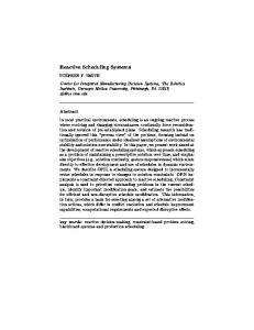
In order to generate a predictive schedule, the total disruption’s repair time per unit time period is calculated for each glaze. To illustrate this procedure, the Regency green glaze, enumerated as g = 1, is considered where the possible occurrences of glaze shortage per unit time period are 1, 2, 3 or 4 with possibilities 0.7, 0.95, 0.4 and 0.25, respectively, i.e., O1 = {0.7/1 + 0.95/2 + 0.4/3 + 0.25/4}, represented in Figure 2. Fuzzy set R1 represents the imprecise repair duration tr1 of material m1 (Regency green glaze), shown in Figure 3. Both fuzzy sets are determined based on the information obtained in the glaze production department at Denby Pottery. Figure 4 shows the level 2 fuzzy set O1 ⊗ R1 , that represents the total disruption repair time per unit time period for glaze m1 = 1, calculated as the product of the two fuzzy sets O1 and R1. Four fuzzy values of the total disruption repair time per unit time period with associated possibilities are presented. Once the total repair duration time per unit time period is calculated as a level 2 fuzzy set, it is transformed into a standard set using s-fuzzification and then defuzzified, leading to the crisp total repair duration time, td1 = 3. In order to find the total disruption’s repair time of Regency green glaze shortage during the processing of a job J1 that uses that specific glaze, td1 is multiplied by the processing time p1 of 80
Alejandra Duenas, Dobrila Petrovic the job. The unit time for the Regency green glaze is 4 hours, and considering job J1 initial processing time p1 = 10, idj is calculated as follows:
id1 =
3 ⋅ 10 = 7.5 hours 4
Therefore, pd1 = 10 + 7.5 = 17.5 hours. This procedure is repeated for each glaze and jobs that might be affected by the shortage of the glaze under consideration. Once, all the processing times are extended by adding the corresponding idle times the schedule that minimises the makespan Cmax is generated.
4.2
Reactive scheduling
In practice, there will be occasions when the disruption cannot be absorbed; for example, if the glaze has low quality and it is impossible to apply it and the glaze production department informs the glazing section leader that the repair time i.e., the time to deliver the glaze is too long. In this case, rescheduling has to be applied. Two rescheduling techniques are proposed: Left-shift rescheduling and Building new schedules as defined in Section 3.
5.
RESULTS ANALYSIS
Two analyses are carried out: (1) to evaluate the effects of the imprecisely specified disruptions on the jobs’ sequence and completion times, (2) to investigate the effects of rescheduling.
5.1
Disruptions impact analysis
The aim of this analysis is to investigate the effects of changing fuzzy repair duration time on the jobs’ sequence and completion times. As defined in Section 4, the total disruption’ repair time per unit time period is determined by the possibility of disruption occurrences per unit time period and the repair duration. The repair duration is linguistically represented as ‘about b to c unit time periods’ and modelled by a fuzzy set with a trapezoidal membership function specified by four parameters a, b, c, and d. In order to analyse the effects of changing the disruption duration period, the parameters a, b, c, and d are varied in two ways: (1) uncertainty in disruption duration period is increased by increasing the distance between b and c and (2) disruption duration period is increased by shifting the domain to the right i.e., by increasing the values of parameters a, b, c and d. 5.1.1
Effect of increasing uncertainty in disruption duration period
Tables 2, 3 and 4 show the jobs’ sequence, completion times and Cmax obtained for three different sets of parameter values: (1) a = 1, b = 2, c = 3 and d = 4, (2) a = 1, b = 2, c = 4 and d = 5, and (3) a = 1, b = 3, c = 6 and d = 8, respectively. As expected, the results obtained showed that changing uncertainty in duration repair period has an adverse impact on the makespan. For example, if the distance between b and c is increased from 1 hour (b = 2 and c = 3) to 2 hours (b = 2 and c = 4) the makespan increases from 88.5 to 98.9 hours, this represents and increment of 10.4 hours (12%). If the distance between b and c is increased from 1 hour (b = 2 and c = 3) to 3 hours (b = 3 and c = 6) the makespan increases from 88.5 to 130 hours, which represents an increment of 41.5 hours (47%). Consequently, it can be concluded that widening the distance between b and c does not have a linear impact on the makespan deterioration. 81
An approach to predictive-reactive scheduling of parallel machines subject to disruptions It may be interesting to analyse the effects of widening the distance between b and c on the glaze disruption’s repair duration per unit time period tdg, g = 1,…,8. It can be seen, in Table 5, that the glaze disruption’s repair duration per unit time period tdg, directly depends on the uncertainty in the repair duration; the more uncertainty in the disruption repair duration, the longer the idle time to be added to the processing time. 5.1.2
The effects of increasing the disruptions duration period
The jobs’ sequence, completion times and Cmax are obtained for three different disruption periods, specified by: (1) a = 2, b = 3, c = 4 and d = 5, (2) a = 3, b = 4, c = 5 and d = 6, and (3) a = 4, b = 5, c = 6 and d = 7 and the results obtained are presented in Tables 6, 7 and 8, respectively. If possible disruption duration periods are increased by 1 hour, i.e., the domain of the corresponding fuzzy set is 1 hour left-shifted, starting from a = 1 to a = 2, the makespan Cmax increases from 88.5 (Table 2) to 98.9 hours (Table 6); this represents an increment of 10.4 hours (12%). Similarly, if the possible disruption periods are increased by 2 hours, i.e., a, b, c, d is changed from a = 1 to a = 3, b = 2 to b = 4, c = 3 to c = 5 and d = 4 to d = 6 the makespan Cmax increases from 88.5 to 108.7 hours, that represents an increment of 20.2 hours (23%). If the increment is 3 hours, i.e., a is changed from a = 1 to a = 4 and all other parameters correspondingly, the makespan Cmax increases from 88.5 to 119.1 hours, and this is an increment of 30.6 hours (35%). Comparing this results with those found when the distance between b and c was increased (Table 2 to Table 6), it appears that the impact of increasing the uncertainty in disruption duration is higher than the impact of increasing the possible disruptions durations. It can also be seen that the jobs’ sequence and completion times when a = 1, b = 2, c = 4 and d = 5 are the same as for a = 2, b = 3, c = 4 and d = 5. It may be of interest to analyse the effects of increasing the possible disruption duration periods on the glazes’ disruption’s repair duration per unit time period tdg (see Table 9). If Table 5 and Table 9 are compared it is possible to see that the impact of increasing uncertainty in disruption duration period, i.e., increasing the distance between b and c is higher than the impact of increasing the possible disruption duration. In other words, increments in uncertainty in the disruption duration periods may cause more changes in the idle times to be added to the processing times than increments in the disruption duration.
5.2
Analysis of rescheduling impact
Two rescheduling methods are proposed: Left-shift rescheduling and Building new schedules. The aim of this analysis is to determine which of these methods yields better results in terms of the two objectives considered, namely efficiency and stability. In order to analyse the impact of rescheduling it is necessary to assume a scenario where high impact disruptions occur. In the scenario under consideration, a bad quality in the Greenwich glaze is detected by the section leader at the moment of producing the first job that involves this glaze. However, the glaze production department is not able to deliver the glaze in a feasible time, and therefore it is necessary to remove all the jobs that use this glaze. Table 10 shows different glazes mg, g = 1,…, 8 considered in this problem, as well as the values of the parameters a, b, c, and d used in order to generate the schedule. As described in Section 4, the disruption’s repair time per unit time period tdg is calculated for each glaze. The jobs’ sequence and completion times are obtained as presented in Table 11. The jobs that use Greenwich glaze are J2, J12 and J22. In terms of starting times, J2 starts processing at 93.7 hours, J12 starts processing at 91.2 hours and J22 starts processing at 89.5 hours. The jobs that use Greenwich 82
Alejandra Duenas, Dobrila Petrovic glaze will be cut off from the schedule and the first job to be removed is job J22. When Left-shifting rescheduling is applied, after the jobs are cut off, the machines where they are expected to be processed (M1 and M3) are treated as single machines. The schedule obtained after applying the Left-shifting rescheduling method is presented in Table 12. As it can be seen, in this case the makespan was not affected since it was determined by machine M2 and this machine was not affected by the disruption. In this case, the objective related to efficiency has not been affected. The next objective to measure is the instability defined by formula (9):
IST ( RS ) =
30
(C j ( PS ) − C j ( RS )) 2 = 166.99
j =1
Since jobs J2, J12 and J22 are cancelled in the reactive schedule RS, in order to calculate IST(RS) the completion times are considered to be equal to zero i.e., C2(RS) = 0, C12(RS) = 0 and C22(RS) = 0. When the Building new schedules method is applied, the new schedule is generated with all the jobs that have not been processed yet, considering the moment of disruption to be the jobs starting time. In the predictive schedule PS (Table 11), the first job affected by the disruption is job J22 which starts processing at 89.5 hours, on machine M3. Jobs J5 and J17 have started being processed and have a completion time of 91.2 and 108.2 hours on machines M1 and M2, respectively. Therefore, the starting time for the new schedule to be built is 91.2 hours for machine M1, 108.2 hours for machine M2 and 89.5 for machine M3. Table 13 shows the schedule obtained after applying the building new schedules method. As it can be seen, in this case the makespan, Cmax=139.6, is smaller than the one found by the Left-shifting rescheduling method, Cmax=144.9. This occurs because the Building new schedule method applies the rules LFJ and LPT which minimise the makespan while the Left-shifting rescheduling method does not consider makespan at all. Additionally, in order to determine which method generates a more stable schedule, the instability of the new schedule is calculated using formula (9) as follows:
IST ( RS ) =
30
(C j ( PS ) − C j ( RS )) 2 = 167.022
j =1
It can be seen that for the efficiency objective (makespan) the rescheduling method that performs better is the building new schedules method, while the Left-shifting method might perform better for the stability/instability objective. It may be concluded that selection of the rescheduling method to be applied depends on which of the objectives considered is more important, the efficiency or stability/instability. Another issue worth considering is the addition of new jobs, as it is often the case in practice that, when a disruption occurs, the production planning department decides to produce some new jobs since some initially planned jobs cannot be produced. In this scenario, for illustrative purposes, it is decided to consider two new jobs with the data given in Table 14: In the Left-shifting rescheduling method, the new jobs can only be added after all the jobs scheduled initially have been completed. Table 15 shows one possible reactive schedule RS with two new jobs J31 and J32, generated using dispatching rules LFJ and LPT. The instability is calculated to be IST(RS) = 166.99. Since jobs J31 and J32 do not exist in the predictive schedule PS, in order to calculate IST(RS) the completion times are considered to be equal to zero i.e., C31(PS) = 0 and C32(PS) = 0. 83
An approach to predictive-reactive scheduling of parallel machines subject to disruptions When the Building new schedules method is applied, the new schedule is generated for all the jobs that have not been processed yet, including the two new jobs J31 and J32, and considering, as the jobs starting time, the moment of disruption. Table 16 shows the schedule obtained after applying the building new schedules method including the two new jobs. Makespan of the schedule Cmax is 153.1 while instability is IST(RS) = 168.89. It can be seen that in this scenario when the two jobs are added, the rescheduling method that yields better results for both objectives, efficiency and instability, is the Left-shifting rescheduling. Hence, the analyses carried out show the importance of selecting the appropriate rescheduling method taking into consideration both the decision maker requirements and preferences, and the objectives to be optimised.
6.
CONCLUSION
A predictive-reactive approach to an identical parallel machine scheduling problem is presented, where a number of jobs has to be processed on parallel machines. The machines are considered to be identical, in other words, the machines have the same speed. The aim of the scheduling is to determine the jobs allocation to the machines and the sequence of the jobs on each machine in the presence of uncertain disruptions in the production environment in such a way as to minimise the makespan. The new approach developed is based on generating a predictive parallel machine schedule using dispatching rules, where the predictive schedule is designed to absorb the effects of a possible uncertain disruption through adding idle times to the jobs’ processing times. Uncertain disruption is specified imprecisely using two parameters, namely number of disruptions occurrences and disruption repair period. They are modelled using fuzzy sets and combined effectively into level 2 fuzzy sets. If the impact of a disruption is too high to be absorbed by the predictive schedule a rescheduling action is needed. The predictive-reactive scheduling approach is applied to a real lifescheduling problem identified in collaboration with a manufacturing pottery company. The use of fuzzy sets in modelling material shortage disruptions proved to be beneficial in this case when there are no historical data and subjective managerial judgement can be used. Two rescheduling methods namely Left-shifting and building new schedules have proven to be of benefit when high impact disruptions occur. The results obtained show that uncertainty in disruptions caused by shortage of a glaze or low quality of the glaze may have a higher impact on the schedule’s execution than repair time, i.e., the time needed for the glaze production department to deliver the glaze. Importance of selecting the appropriate rescheduling method, according to the decision maker requirements and preferences, and the objectives to be optimised is demonstrated. The results obtained using the rescheduling methods are satisfactory and showed the model’s flexibility since the rescheduling methods can also be used when new jobs arrive. Further work will be undertaken including: – Investigation of different techniques to measure level of uncertainty, represented by fuzzy sets in order to quantify the impact of uncertain disruptions on the schedule performance, – Development of a decision-making method for determining whether to perform rescheduling at a particular disruption and which rescheduling method to use, – Development of a simulation model of realised schedules in order to measure the level of predictability of the predictive schedule, i.e., the quality of the schedule in terms of absorbing the effects of a disruption. – Analysis of possible improvements in scheduling that might be gained at the pottery company by using the method proposed.
84
Alejandra Duenas, Dobrila Petrovic
ACKNOWLEDGEMENTS This research is supported by Engineering and Physical Sciences Research Council (EPSRC), grant no. GR/R95326/01. This support is gratefully acknowledged. We also acknowledge the support of the industrial collaborator the Denby Pottery Company Ltd.
APPENDIX Definition of a fuzzy set [12]. Let X denotes a universal set with elements denoted as x. A fuzzy set A in X is characterised by a membership function µA(x), where µA(x):X→[0,1] associates each element x with a degree of membership of x in A. In the case when x is discrete and finite x = {x1 , x2 , , xk } , fuzzy set A may be denoted by A = A = µ A ( x) / x .
K
µ A ( xk ) / xk . When X = {x} is continuous, fuzzy set A may be represented by
k =1
x
REFERENCES 1. 2. 3. 4. 5. 6. 7. 8. 9. 10. 11. 12. 13. 14.
Pinedo M., Scheduling: Theory, Algorithms, and Systems, Prentice Hall, 2002. Vieira G.E., Herrmann J.W., Lin E., Rescheduling manufacturing systems: a framework of strategies, policies, and methods, Journal of Scheduling, Vol. 6, pp. 39-62, 2003. Aytug H., Lawley M.A., McKay K., Mohan S., Uzsoy R., Executing production schedules in the face of uncertainties: A review and some future directions, European Journal of Operational Research, Vol. 161, pp.86-110, 2005. O’Donovan R., Uzsoy R., McKay K.N., Predictable scheduling of a single machine with breakdown and sensitive jobs, International Journal of Production Research, Vol. 37, No. 18, pp. 4217-4233, 1999. Mehta S.V., Uzsoy R., Predictable scheduling of a single machine subject to breakdowns, International Journal of Computer Integrated Manufacturing, Vol. 12, No. 1, 15-38, 1999. Li H., Li Z., Li L.X. Hu B., A production rescheduling expert simulation system, European Journal of Operational Research, Vol. 124, pp. 283-293, 2000. Abumaizar R.J., Svestka J.A., Rescheduling job shops under random disruptions, International Journal of Production Research, Vol. 35, No. 7, pp. 2065-2082, 1997. Rangsaritratsamee, R., Ferrell W.G., Kurz M.B., Dynamic rescheduling that simultaneously considers efficiency and stability, Computers and Industrial Engineering, Vol. 46, pp. 1-15, 2004. Ruspini E.H., P.P. Bonissone and W. Pedrycz, Handbook of Fuzzy Computation, Institute of physics publishing, USA, 1998. Zimmermann H–J., Fuzzy Set Theory-and Its Applications, Third Edition, Kluwer Academic Publishers, 1996. Petrovic D., Petrovic R., Vujosevic M., Fuzzy models for the newsboy problem, International Journal of Production Economics, Vol. 45, pp. 435-441, 1996. Zadeh L.A., Fuzzy Sets, Information and Control, Vol. 8, pp. 338-353, 1965. Panwalkar S.S, Iskander W., A survey of scheduling rules, Operations Research, Vol. 25, No. 1, pp. 45-61, 1977. Papoulis A., Probability, random variables and stochastic processes, Third Edition, McGraw-Hill, Inc., 1991.
85
An approach to predictive-reactive scheduling of parallel machines subject to disruptions Table 1. Identical parallel machine scheduling data for 10 jobs job Jj pattern item unit time processing M1 (hours)/ 100 time pj (hours) items 1 Regency green Large Jug 4 10 2 Greenwich 4 2 Large Jug 3 Marrakesh 6 5 Sauce Boat 4 7 4 Regency green Teapot Base 5 Fire 5 2 Small Jug 6 Energy 3 3 Teapot (Classic) 7 Harlequin 8 Small Teapot Base 4 4 8 Spirit Large Teapot Base 6 9 Fire 5 1 Large Jug 10 Blue Jetty 4 6 Sauce Jug
M2 M3 × ×
×
× ×
Table 2. Jobs’ sequence, completion times and Cmax when a = 1, b = 2, c = 3 and d = 4 machine jobs’ sequence M1 20 21 11 22 12 25 5 9 4 M2 27 17 7 24 28 18 3 M3 30 10 1 2 15 29 19 14 8 machine completion times M1 M2 M3
18.0
31.5
45.0
48.0
51.0
54.0
57.0
16.0
32.0
48.0
58.5
68.5
78.5
86.0
18.0
36.0
49.5
52.5
55.5
57.0
58.5
Cmax =
88.5
23
13
26
16
58.5
69.0
76.5
84.0
69.0
79.0
83.5
88.0
Table 3. Jobs’ sequence, completion times and Cmax when a = 1, b = 2, c = 4 and d = 5 machine jobs’ sequence M1 20 21 11 25 15 22 2 19 M2 27 17 7 28 8 4 26 16 M3 30 10 1 5 12 29 9 24 machine M1 M2 M3 Cmax =
88.5
18
14
3
23
13
6
76.4
87.7
95.9
85.9
94.0
98.9
completion times 21.0
35.6
50.2
53.5
56.7
60.0
63.2
64.9
18.0
36.0
54.0
65.5
77.0
88.4
93.2
98.1
21.0
42.0
56.6
59.9
63.1
64.7
66.4
77.7
98.9
Table 4. Jobs’ sequence, completion times and Cmax when a = 1, b = 3, c = 6 and d = 8 machine jobs’ sequence M1 20 21 11 25 22 15 12 2 M2 27 17 7 28 8 23 13 6 M3 30 10 1 5 29 19 18 4 machine completion times M1 M2 M3 Cmax =
6
30.0
48.0
66.0
70.0
74.0
78.0
82.0
86.0
24.0
48.0
72.0
88.0
104.0
114.0
124.0
130.0
30.0
60.0
78.0
82.0
84.0
86.0
102.0
116.0
130
86
9
24
26
16
88.0
102.0
122.0
128.0
14
3
116.0
126.0
Alejandra Duenas, Dobrila Petrovic Table 5. Glaze disruption’s repair duration per unit time Glaze mg pattern g 1 2 3 4 5 6 7 8
tdg (hours) a = 1, b = 2, c = 4 and d = 5 2.5 2.5 2.5 2.5 2.5 5 7.5 10
a = 1, b = 2, c = 3 and d = 4 2 2 2 2 2 4 6 8
Regency green Greenwich Marrakesh Fire Energy Harlequin Spirit Blue Jetty
Table 6. Jobs’ sequence, completion times and Cmax when a = 2, b = 3, c = 4 and d = 5 machine jobs’ sequence M1 20 21 11 25 15 22 2 19 M2 27 17 7 28 8 4 26 16 M3 30 10 1 5 12 29 9 24 machine completion times M1 M2 M3 Cmax =
21.0
35.6
50.2
53.5
56.7
60.0
63.2
64.9
18.0
36.0
54.0
65.5
77.0
88.4
93.2
98.1
21.0
42.0
56.6
59.9
63.1
64.7
66.4
77.7
14
3
23
13
6
76.4
87.7
95.9
85.9
94.0
98.9
24
14
3
97.5
106.2
16
85.2
108.2
108.7
Table 8. Jobs’ sequence, completion times and Cmax when a = 4, b = 5, c = 6 and d = 7 Machine jobs’ sequence M1 20 21 11 25 15 5 12 29 19 M2 27 17 7 28 24 14 3 M3 30 10 1 22 2 9 8 23 13 machine completion times M1 M2 M3 Cmax =
18
98.9
Table 7. Jobs’ sequence, completion times and Cmax when a = 3, b = 4, c = 5 and d = 6 machine jobs’ sequence M1 20 21 11 25 15 5 12 29 9 M2 27 17 7 28 8 23 13 6 M3 30 10 1 22 2 19 18 4 26 machine completion times M1 24.0 39.7 55.5 59.0 62.5 66.0 69.5 71.2 73.0 M2 20.0 40.0 60.0 73.0 86.0 94.7 103.5 108.7 M3 24.0 48.0 63.7 67.2 70.7 72.5 85.5 97.7 103.0 Cmax =
a = 1, b = 3, c = 6 and d = 8 4 4 4 4 4 8 12 16
27.0
43.9
60.8
64.5
68.3
72.0
75.8
22.0
44.0
66.0
80.5
93.6
106.7
116.1
27.0
54.0
70.9
74.6
78.4
80.3
94.8
119.1
87
18
4
26
16
107.1
112.7
118.4
6
77.6
79.5
94.0
104.1
113.5
119.1
An approach to predictive-reactive scheduling of parallel machines subject to disruptions Table 9. Glaze disruption’s repair duration per unit time glaze mg pattern
1 2 3 4 5 6 7 8
tdg (hours) a = 3, b = 4, c = 5 and d = 6 3 3 3 3 3 6 9 12
a = 2, b = 3, c = 4 and d = 5 2.5 2.5 2.5 2.5 2.5 5 7.5 10
Regency green Greenwich Marrakesh Fire Energy Harlequin Spirit Blue Jetty
Table 10. Glazes considered glaze mg pattern g 1 Regency green 2 Greenwich 3 Marrakesh 4 Fire 5 Energy 6 Harlequin 7 Spirit 8 Blue Jetty
Table 11. Predictive schedule PS machine M1 11 30 M2 24 14 M3 21 1 machine M1 M2 M3 Cmax =
a = 4, b = 5, c = 6 and d = 7 3.5 3.5 3.5 3.5 3.5 7 10.5 14
a
b
c
d
2 1 5 4 1 3 8 1
5 2 8 8 3 6 12 2
7 3 13 14 6 11 16 5
10 4 16 18 9 13 20 6
tdg (hours) 9 4.5 6.5 10 3 6 9 12
jobs’ sequence 20
25
5
4
27
17
13
28
26
6
10
15
22
2
19
7
18
16
128.7
12
29
9
23
3
8
completion times 29.2
53.2
77.2
84.2
91.2
95.5
99.0
102.5
115.6
22.7
45.5
68.2
88.2
108.2
121.4
134.4
139.6
144.9
29.2
58.5
82.5
89.5
93.7
98.0
101.5
121.5
134.5
139.7
23
3
8
26
6
144.9
Jobs that use Greenwich glaze
Table 12. Schedule RS obtained after Left-shifting rescheduling machine jobs’ sequence M1 11 30 20 25 5 29 9 M2 24 14 4 27 17 13 28 M3 21 1 10 15 19 7 18 machine completion times M1 M2 M3 Cmax =
16
29.2
53.2
77.2
84.2
91.2
94.7
98.2
111.3
124.4
22.7
45.5
68.2
88.2
108.2
121.4
134.4
139.6
144.9
29.2
58.5
82.5
89.5
93
113
126
131.2
144.9
88
137.4
141.7
Alejandra Duenas, Dobrila Petrovic Table 13. Schedule RS obtained after applying building new schedules method machine jobs’ sequence M1 11 30 20 25 5 19 7 M2 24 14 4 27 17 13 18 M3 21 1 10 15 29 9 23 machine completion times M1 M2 M3 Cmax =
28
26
16
6 3
8
132.9
29.2
53.2
77.2
84.2
91.2
94.7
114.7
127.7
22.7
45.5
68.2
88.2
108.2
121.3
134.3
139.6
29.2
58.5
82.5
89.5
93
96.5
109.6
122.7
135.7
139.6
Table 14. Added jobs job Jj pattern
item
31 32
Large Jug Sauce Boat
Regency green Marrakesh
unit time (hours) 4 6
initial processing times pk (hours) 8 6
Table 15. Schedule RS obtained using Left-shifting rescheduling with two new jobs J31 and J32 machine jobs’ sequence M1 11 30 20 25 5 29 9 23 3 8 M2 24 14 4 27 17 13 28 26 6 M3 21 1 10 15 19 7 18 16 31 machine M1 M2 M3 Cmax =
M1
53.2
77.2
84.2
91.2
94.7
98.2
111.3
124.4
22.7
45.5
68.2
88.2
108.2
121.4
134.4
139.6
144.9
32
29.2
58.5
82.5
89.5
93
113
126
131.2
149.2
137.4
144.9
149.2
29.2
53.2
77.2
84.2
91.2
94.7
98.2
101.7
22.7
45.5
68.2
88.2
108.2
124
137.1
150.1
29.2
58.5
82.5
89.5
115.5
128.6
141.6
146.9
153.1
89
121.7
152.1
M2 ×
completion times 29.2
Table 16. Schedule RS obtained using Building new schedules with two new jobs J31 and J32 machine jobs’ sequence M1 11 30 20 25 5 29 19 9 7 M2 24 14 4 27 17 32 3 8 M3 21 1 10 15 31 23 28 26 16 machine completion times M1 M2 M3 Cmax =
138.2
13
18
6
134.8
147.8
153.1
M3
An approach to predictive-reactive scheduling of parallel machines subject to disruptions
membership degree
membership degree
1
noc1 noc2 noc3
noc4 number of
a
disruptions per unit time period
(a) Fuzzy number of disruptions per unit time period
b
c
d
disruption time
(b) Fuzzy disruption time
Figure 1. Fuzzy sets that represent an uncertain disruption
µO1 (noc1 ) 0.95 0.7 0.4 0.25
1
2
3
noc1
4
Figure 2. Fuzzy set O1 that represents an imprecise number of disruption occurrences per unit time period
µ R1 (tr1)
1
2
3
4
tr1
Figure 3. Fuzzy set R1 that represents an imprecise repair duration
90
Alejandra Duenas, Dobrila Petrovic
µ1×~ R1 (tr1 )
µ 2~× R1 (tr1 ) 1
1
0
0
2
1
4
3
tr1
2
(a) Fuzzy total repair duration, possibility 0.7
6
8
tr1
(b) Fuzzy total repair duration, possibility 0.95
µ 4~× R1 (tr1 )
µ 3×~ R1 (tr1 ) µ
4
(1) ⋅ µ
µ
(tr )
1
⋅µ 1
0
0
3
6
9
12
tr1
(c) Fuzzy total repair duration, possibility 0.4
4
8
12
16 tr1
(d) Fuzzy total repair duration, possibility 0.25
Figure 4. The fuzzy values of the total disruption’s repair time for Regency green glaze and the associated possibilities
91