SMC-4, July 1974. [14] K. S. Narendra and M. A. L. Thathachar, Learning Automata. Engle- wood Cliffs, NJ: Prentice-Hall, 1989. [15] K. Naruse and Y. Kakazu, ...
128
IEEE TRANSACTIONS ON SYSTEMS, MAN, AND CYBERNETICS—PART A: SYSTEMS AND HUMANS, VOL. 29, NO. 1, JANUARY 1999
[9] C. Marsh, T. J. Gordon, and Q. H. Wu, “Stochastic optimal control of active vehicle suspensions using learning automata,” in Proc. Mech. Eng. Part I, J. Syst. Contr. Eng., vol. 207, pp. 143–152, 1993. [10] K. Nagel and S. Rasmussen, “Traffic at the edge of chaos,” in Artificial Life IV. Cambridge, MA: MIT Press, 1994, pp. 222–235. [11] K. Najim, “Modeling and self-adjusting control of an absorption column,” Int. J. Adap. Contr. Signal Process., vol. 5, pp. 335–345, 1991. [12] K. Najim and A. S. Poznyak, Eds., Learning Automata: Theory and Applications. Oxford, U.K.: Elsevier, 1994. [13] K. S. Narendra and M. A. L. Thathachar, “Learning automata—A survey,” IEEE Trans. Syst., Man, Cybern., vol. SMC-4, July 1974. [14] K. S. Narendra and M. A. L. Thathachar, Learning Automata. Englewood Cliffs, NJ: Prentice-Hall, 1989. [15] K. Naruse and Y. Kakazu, “Strategy acquisition of path planning of redundant manipulator using learning automata,” IEEE Int. Workshop Neuro-Fuzzy Ctrl., 1993, pp. 154–159. [16] M. F. Norman, Markov Processes and Learning Models. New York: Academic, 1972. [17] B. J. Oommen and E. V. de St. Croix, “String taxonomy using learning automata,” Tech. Rep. TR-234, School of Computer Science, Carleton Univ., Ottawa, Ont., Canada, Mar. 1994. [18] M. L. Tsetlin, Automaton Theory and Modeling of Biological Systems, Vol. 102 in Mathematics in Science and Engineering. New York: Academic, 1973. ¨ [19] C. Unsal, “Intelligent Navigation of Autonomous Vehicles in an Automated Highway System: Learning Methods and Interacting Vehicles Approach,” Ph.D. dissertation, Virginia Tech., Blacksburg, Jan. 1997, (http://www.theses.org/). [20] P. Varaiya, “Smart cars on smart roads: Problems of control,” IEEE Trans. Automat. Contr., vol. 38., pp. 195–207, Feb. 1993.
Semantic Constraints for Membership Function Optimization J. Valente de Oliveira
Abstract—The optimization of fuzzy systems using bio-inspired strategies, such as neural network learning rules or evolutionary optimization techniques, is becoming more and more popular. In general, fuzzy systems optimized in such a way cannot provide a linguistic interpretation, preventing us from using one of their most interesting and useful features. This work addresses this difficulty and points out a set of constraints that when used within an optimization scheme obviate the subjective task of interpreting membership functions. To achieve this a comprehensive set of semantic properties that membership functions should have is postulated and discussed. These properties are translated in terms of nonlinear constraints that are coded within a given optimization scheme, such as backpropogation. Implementation issues and one example illustrating the importance of the proposed constraints are included. Index Terms—Adaptive systems, fuzzy systems, learning, membership functions, neural networks, optimal interfaces, optimization, semantic constraints.
I. INTRODUCTION When compared with other nonlinear modeling techniques such as artificial neural networks, Hammerstein, Wiener, or more generally NARMAX models (cf. [3]), fuzzy systems have the important adManuscript received April 15, 1996; revised February 10, 1997 and April 10, 1998. The author is with the Department of Mathematics and Computer Science, Universidade Da Beira Interior, 6200 Covilh˜a, Portugal. Publisher Item Identifier S 1083-4427(99)00895-4.
vantage of providing an insight on the linguistic relationship between the variables of the system. In the context of approximation tasks, the optimization of fuzzy systems (such as controllers, models, or classifiers) using biological inspired strategies (such as neural networks learning rules, or evolutionary optimization techniques like genetic algorithms) is becoming more and more popular. What is common in these bioinspired strategies is that the only indicator guiding the search process is concerned exclusively with the system quality in terms of the approximation task (e.g., with the errors between system output and training data). For example, this is case with the so-called performance index of the neural networks learning rules [7] and with the fitness function of the genetic algorithms [5]. In the presence of such unconstrained optimization processes the parameters of membership functions (e.g., centers and widths) are treated just like any other parameter of the system. Furthermore, usually a fuzzy system has very many independent parameters (degrees of freedom). As a consequence, several local minima of the performance function are likely to exist. In face of this we simply cannot ensure that the resulting membership functions have any semantic value in what concerns their ability to be interpretable as linguistic terms. To ignore this aspect during fuzzy system design is first of all to renounce the richness of concepts and techniques provided by fuzzy sets and systems. It is comparable to let the fuzzy parameters outgoing their range (usually [0, 1]) violating the set or logic nature of fuzzy calculus. It is equivalent to consider fuzzy systems as a tool for initializing artificial neural networks (in the sense that without semantics a fuzzy system can be viewed as a neural net). While this is undebatable, one may legitimately ask 1) whether constraining the optimization to preserve semantics would not degrade the fuzzy system performance, and 2) what would be the reasons to translate the functioning of, e.g., a ready-to-implement fuzzy control algorithm into a natural-language equivalent description. For addressing the first issue, it is recalled that, in general, unconstrained optimization methods are more susceptible to get stuck in local minima than conveniently constrained ones. One the other hand, minima are necessarily local in that region of parameters space where there is no possible interpretation. A typical case being the absence of membership functions in a subset of the universe of discourse. This being so, there would be input values for which the system would have no response. Constraints may help to avoid local minima. The systematic avoidance of local minima leads to the global minimum, and thus to optimal performance. This contradicts the naive belief that constrained optimization cannot perform better than unconstrained optimization. Take adaptive control as an example. In certain model-reference schemes unconstrained optimization of the controller gains leads to unstable closed-loop responses. However when equipped with convenient constraints, these control schemes leads to guaranteed stability, cf. [1]. Later on, this semantics/performance synergy is further illustrated by means of an included example where a fuzzy system optimized with semantic constraints performs better than other with the same structure and initial conditions, but optimized without taking care of semantics. Notice also that the first applied fuzzy (control) systems were designed using heuristic methods based on the knowledge and experience of experts, and thus they were necessarily semantically valid. However this has not degraded their performances; by the opposite in
1083–4427/99$10.00 1999 IEEE
IEEE TRANSACTIONS ON SYSTEMS, MAN, AND CYBERNETICS—PART A: SYSTEMS AND HUMANS, VOL. 29, NO. 1, JANUARY 1999
many cases better performances were obtained when compared with the other available solutions, cf. [14]. For addressing the second issue, we can consider an industrial plant where a new variable was made observable to improve the performance of an existent fuzzy controller. In this case, the maintenance of the controller will be easier to accomplish by someone who finds a set of legible if–then rules instead of a set of meaningless parameters such as those found in neural networks. While it is very difficult to include additional functionality in a trained neural network, it is relatively easy to add, e.g., a new production rule into a trained legible fuzzy system. On the other hand, for those fuzzy systems dealing with user interfaces using a natural language, semantics is a crucial requirement. The fuzzy I/O controller is one of such systems [14]. This work is devoted to the study of semantically driven conditions to constraint the optimization process of a fuzzy system in such a way that the resulting membership functions can still represent human readable linguistic terms. In Section II, a comprehensive set of semantic properties membership functions should meet is postulated and discussed. In Section III, constraints are introduced and analyzed. Section IV discusses some implementation issues, and presents one example illustrating the importance of the proposed constraints. A section on conclusions ends the paper. II. ON MEMBERSHIP FUNCTIONS AND LINGUISTIC TERMS Conceptually the architecture of a fuzzy system involves three different stages: the so-called input interface, the fuzzy processing stage, and the output interface. An interface deals with linguistic variables. The notion of linguistic variable formally requires a semantic rule for associating a meaning to each one of its values, the linguistic terms represented by the referential or primary fuzzy sets [20]. Hence, each referential fuzzy set should represent a linguistic term with a clear semantic meaning. If the system processes the linguistic variable temperature, then its values might be “high,” “medium,” and “low” temperature, for instance. In this section, an attempt is made to postulate a set of properties that the membership functions of the referential fuzzy sets should have to obviate the subjective task of assigning linguistic terms to them. The focus is on the meaning of a linguistic term within its context i.e. relatively to the other linguistic terms, instead of on the absolute meaning of an isolated linguistic term. The set of semantic properties includes, cf. [16]. A moderate number of membership functions, distinguishability, normality, natural zero positioning, and coverage.
129
fields. The problem is that above this number the errors generated by us while juggling, dealing with, or handling objects, entities, or concepts rise in a strong nonlinear way. Thus we can and should adopt this typical number as an upper-bound on the number of membership functions. Curiously enough, it is interesting to verify that most of the successful industrial and commercial applications of fuzzy systems do not exceed this limit, cf. [14]. B. Distinguishability By definition of linguistic variable, there should be a semantic rule associating a meaning to each value of the variable. That is, a membership function should represent a linguistic term with a clear semantic meaning. To obviate the subjective establishment of this membership functions/linguistic term association, membership functions of a given linguistic variable should be distinct enough from each other. In the absence of this property, a variable could have equal membership functions what would be superfluous, tautological, and misleading. The existence of close or nearly identical membership functions (linguistic terms) may cause inconsistencies at the processing stage. As an illustration, consider, e.g., the following fuzzy rules: IF A THEN B and IF A0 THEN C; where A; A0 ; B; and C are linguistic terms. If A and A0 are nearly identical then an inconsistency is likely to happen, since for the same input two distinct conclusions, induced by B and C; are derived. If required, fine shades of meaning can be realized at the processing stage using logical connectives (such as conjunction and negation) and hedges (such as very) on the linguistic terms [19], [20]. C. Normality Membership functions should be normal. Since each membership function should represent a linguistic term with a clear semantic interpretation, then at least one of the datum in the universe of discourse should exhibit full matching with each membership function. More formally
9
v2V
8 =1 2
; ;111;n �i (v)
i
= 1:0
(1)
where v is any external variable defined in V ; n is the number of membership functions and �i is the ith membership function. Semantically consider nonnormal membership functions is to question the meaning of the represented linguistic terms. On the other hand, normality allows one to use the entire range of membership grades, usually [0, 1]. D. Natural Zero Positioning
A. A Moderate Number of Membership Functions The number of membership functions should not be arbitrary. Although this number has been recognized as application dependent, there are some reasons for imposing an upper bound on the number of membership functions. The main reason pertains to the Zadeh’s principle of incompatibility [19]. As soon as the number of membership functions increases the precision of the system may increase too, but its relevance will decrease. In the limit, when the number of membership functions approaches the number of data, a fuzzy system becomes a numeric system. What would be then an appropriated limit? A well-known and interesting result from Cognitive Psychology is that the typical number of different entities efficiently handled at the short-term memory (also known as active, or working memory) is 7 6 2 [9]. See also [9]. This observation on the human information process limitations has guided most of the strategies for segmenting, factoring, or decomposing problems in Computer Sciences and other
If required by the nature of the problem, one of the membership functions should be unimodal, convex, and centered in zero, representing the linguistic term nearly zero. This applies to most fuzzy controllers essentially because a nearly zero tracking error (exactly zero, if possible) is desirable. It should be emphasized the difference between the location of the linguistic term nearly zero, and its necessity for solving a given problem. E. Coverage
Membership functions �i of the referential sets Xi should cover the entire universe of discourse, so that every piece of data may have a linguistic representation. Formally
8
v2V
9:1 i
�i�n �i (v) >
0:
(2)
More generally, one may defined a certain level of coverage, �; given raise to the concept of strong coverage, as follows:
8
v2V
9 :1 i
�i�n �i (v) >
�:
(3)
130
IEEE TRANSACTIONS ON SYSTEMS, MAN, AND CYBERNETICS—PART A: SYSTEMS AND HUMANS, VOL. 29, NO. 1, JANUARY 1999
This property is closely related to completeness. Completeness is a property of deductive systems (or theories) that has been used in the context of Artificial Intelligence to indicate that the knowledge representation scheme can represent every entity within the intended domain. When applied to fuzzy systems, and informally, this property states that a fuzzy system should be able to derive a proper action for every input [8]. Obviously, if a given region of the UoD is not cover by any membership function then fuzzy system cannot take any action for an input in that region. Even for the case in which the system is required to take no action, this should be explicitly handled at the processing stage. For instance, using a rule such as IF x is X THEN y is Z E; where x represents the state of the system, X; is an intended linguistic term, y represents the output of the system, and ZE is the nearly zero linguistic term. III. CONSTRAINTS
FOR
(a)
SEMANTIC INTEGRITY
In this section, a set of constraints able to ensure the postulated semantic properties is given. Some of the semantic properties of membership function can be satisfied easily by an a priori selection of certain membership function features. This is the case with the number of membership functions, and the use of normal membership functions, or even by forcing a membership function to be positioned at zero, if required. However the coverage and distinguishability properties should be monitorized and enforced during the optimization process of the overall system. (b)
A. Constraints for Coverage To ensure coverage one could use a constraint based directly on condition (3). This constraint can be expressed in terms of the sigma-count measure of the internal representation of the data. The sigma-count gives a measure of the cardinality of a fuzzy set A; as follows [7]: Mp (A) =
p
p
a 1 + 1 1 1 + an
(4)
where ai (i = 1; 1 1 1 ; n) are the degrees of membership defining the fuzzy set A: Therefore (3) can be ensured by 8
v
2V Mp (L(v)) > �
(5)
where L(v) gives the internal representation of the extern variable v; a fuzzy (sub)set. Another more general constraint is based on the concept of optimal interfaces. This concept, introduced in [15], and further analyzed in [16], can be presented as follows. Definition 1: Let V = [a; b] � or 8v2V Mp Lv v > : Notice that this proposition does not dependent on the conversion methods used at the input or at the output interfaces. On the other hand, a strong form of coverage can be assured as soon as both Lv and Nv have been specified. For backing up this claim, one can show that for triangular membership functions and for the COG defuzzification method, (6) assures a level of coverage of 0.5. Let
( ( )) = : () 0
( ( )) 0
Lv = [1(v; C1 ; W1 ) 1(v; C2 ; W2 )]
0
be the mapping provided by an input interface, where represents the ith membership function, given by
1(v; Ci ; Wi ) = 1i (v) = 1 0 jv 0 Ci j 0 1( ;
) 1 )
Wi
(9)
1(v; Ci ; Wi )
i = 1; 2
(10)
such that � v Ci ; Wi � as illustrated in Fig. 2. Proposition 2: Let Lv ; Nv be a pair of interfaces where Lv is given by (9) with triangular membership functions 1 ; 2 defined in V a; b ; the operator Nv is given by the COG method. If Lv ; Nv satisfies (6) then 1 ; 2 ensures a coverage level of 0.5. Proof: Under the conditions of the proposition it follows that
=[ ]
(
1 1
1 1
8v
[a b]
2
that can be rewritten as
violates (6)
C2 = C1 ) 8v
= C1 _ v = C2 : = C1 we have 11 (v = C1 ) = 1 ^ 12 (v =
11 (v)C1 + 12 (v)C2 = v 11 (v) + 12 (v)
(
)
(11)
11 (v)[C1 0 v] + 12 (v)[C2 0 v] =0; (12) 11 (v) + 12 (v) 6= 0: If v = C1 then from (12) 12 (v )[C2 0 C1 ] = 0; i.e., 12 (v ) = 0 _ C2 = C1: Notice that, C2 = C1 is an invalid solution since it
[a b] v
2
Therefore, for v : Moreover, from
C1 )
=0
12 (v = C1 ) = 1 0 jC1W02C2 j = 0 (13) it comes that W2 = jC1 0 C2 j ^ W2 6= 0: Similarly, if v = C2 then 11 (v = C2 ) = 0:0; 12 (v = C2 ) = 1:0; W1 = jC2 0C1 j: Thus W1 = W2 = jC1 0C2 j = jC2 0C1 j =6 0:
Now solving an equation system resulting from replacing successively v by a and b (the extremes of UoD) in (12), i.e., solving
( ) = 0
( ) =
131
=
1 0 jCja100CC12jj (C1 0 a) + 1 0 jCja100CC22jj (C2 0 a) = 0 1 0 jCjb100CC12j j (C1 0 b) + 1 0 jCjb100CC22j j (C2 0 b) = 0 =
it comes C1 a ^ C2 b; and thus membership functions are therefore
W1
(14)
= W2 = ja 0 bj: The
11 (v) = max 0; 1 0 jjva 00 abjj 12 (v) = max 0; 1 0 jjav 00 bbjj
:
(15)
The intersection of these functions gives a degree of coverage of 0.5. Corollary 1: Let Lv ; Nv be a pair of interfaces where Lv is given by (9) with triangular membership functions 1 ; 2 defined in V a; b ; the Nv operator given by the COG method. If Lv ; Nv satisfies (6) then the two fuzzy sets form a fuzzy partition of the UoD, in the strict sense, i.e.,
(
)
1 1
=[ ]
(
)
8v V 11 (v) + 12 (v) = 1:0 2
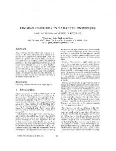
Proof: It follows from the sum, in the UoD, of the functions (15). In plain words, under the conditions of the Corollary 1, the membership functions represent linguistic terms that can be interpreted as partitioning the UoD with the intuitive notions of small and large, as shown in Fig. 3. A straightforward (but not unique) way of generalizing the result of Proposition 2 for a generic number, n, of membership functions is to split the UoD (the interval a b into n 0 subintervals, and use the membership functions determined in the previous proof to assign pairs of membership functions. This is shown in Fig. 4.
[
])
1
132
IEEE TRANSACTIONS ON SYSTEMS, MAN, AND CYBERNETICS—PART A: SYSTEMS AND HUMANS, VOL. 29, NO. 1, JANUARY 1999
3) On Implementation: Condition (6) provides a simple constraint allowing an efficient implementation. In this respect, and from a practical stand point (i.e., assuming that we are using digital computers) we can consider that the UoD of a given variable is represented by a ; 1 1 1 ; N; discretized according sequence of samples, say fx k g k to some appropriated sampling criterion used in the context of the problem to be solved by the overall system. Therefore condition (6) gives rise to the following nonlinear constraint:
[ ] =1
J1 = 12
Fig. 4. Triangular membership functions satisfying the concept of optimal interfaces show a 0.5 degree of coverage.
2) On Information Equivalence: Condition (6) is a sufficient condition for ensuring equivalence between external (data presented to the overall system) and the internal (data processed by the fuzzy processing unit) formats of information [16], i.e., 8v ;v 2V v 0 6
v
00
:
) L (v ) 6= L (v ): v
0
00
v
=
where
x�[k] is given by
x
v
1( )
=[ ]
with all the membership functions i v defined in V a; b and such that 1) In each point v 2 V only two functions are nonnull, 2) two consecutive functions overlap at 0.5, and 3) the following boundary conditions are satisfied 1 v a : 1v b : and n v b : nv a : : The Nv operator is given by the COG method. Under these conditions Lv ; Nv satisfies the optimal interfaces criterion (6). Proof: Since the membership functions i v i ; 1 1 1 ; n are normal and unimodal, from the boundary conditions the extremes a and b are the centers of 1 v and n v ; C1 and Cn , respectively. That is, a C1 < C2 < 1 1 1 < Cj < 1 1 1 < Cn b: Between any two consecutive centers Cj ; Cj +1 with j ; 1 1 1 ; n 0 there are only two membership functions, and these are defined by the equations
1 ( = ) = 1 0(1 ( = ) = 1 ( = ) = 1 0(1 ( = ) = 0 0) ( ) 1 ( ); = 1 1() 1() = = =1 1
0 0)
j
C +1 = 0 C +110 C v + C +1 0C j
j
j
j
x
�2 (x)
x
yj +1 =
[
]
1
Cj +1 0 Cj
v0
[
(16)
n
=
=1
Cj Cj +1 0 Cj
(17)
yj Cj + yj +1 Cj +1 yj + yj +1
C +1 0 C +110 C v + C +1 0C
n
�i (x)
=v
j
(21)
where ai is the mean (or modal) value of the ith membership function in (20). Appendix A includes the details required for the implementation of this constraint. B. Constraints for Distinguishability For ensuring distinguishability we will adopt a constraint on the region of the hypercube where the internal (fuzzy) representation of the fuzzy system may exist. This can be done using again the sigma-count measure. As a brief motivation consider two membership functions, say �i and �j ; very close to each other. In this case, there will be a certain x in the UoD for which its internal representation will have components �i x and �j x with about the same high value, as shown in Fig. 5. On the other hand, if the membership functions are far enough, these components will not have simultaneously high values for none of the elements in the UoD. We can formalize this reasoning in the following constraint:
()
()
V Mp (Lv (v)) � 1:
(22)
Notice that asking for a sigma-count always strictly less than 1 is not feasible since we are assuming normal membership functions. On the other hand, asking for a sigma-count greater than 1 is equivalent to remove the constraint. The parameter p in (22) is used for controlling the strength of the constraint. For p we have a strong constraint whereas it can be eliminated as p ! 1: Appendix B includes the detailed formulae required for the implementation of this constraint.
=1 +
1 1
Cj Cj +1 C j j j j +1 0 Cj Cj +1 Cj 0 Cj+110 Cj v + Cj+1 0 Cj + Cj+1 0 Cj v 0 Cj+1 0 Cj j
=
(20)
�i (x)ai
i
=1
8
]
v� =
0
x� = Nx (Lx (x))
j
valid in Cj ; Cj +1 : According to the COG method, the converted value v for v 2 Cj ; Cj +1 is shown in (18) at the bottom of the page. This result is a formal reason for using this type and distribution of membership functions (Fig. 4), which are quite common in the applications of fuzzy sets and systems (e.g., [8] and [14]).
�
�n (x)]
and Nx can be given by any differentiable defuzzification method, such as the COG. Thus
v2
and
111
i
0
n
(19)
=1
L (x) = [�1(x)
)
L = [11 (v) 1 1 1 1 (v)]
k
(x[k] 0 x�[k])2
N (L (x)): Let
In this respect, it should be stressed that (6) excludes the commonly used trapezoidal membership function distribution, while it elects triangular membership functions with 0.5 of overlapping as able of meeting the criterion (6). This does not means that input or output interfaces have to provide linear mappings. Proposition 3: Let Lv ; Nv be a pair of interfaces where
(
N
Cj +
Cj +1 0 Cj
v0
(18)
IEEE TRANSACTIONS ON SYSTEMS, MAN, AND CYBERNETICS—PART A: SYSTEMS AND HUMANS, VOL. 29, NO. 1, JANUARY 1999
133
B. Example Most fuzzy systems are involved in approximation tasks (e.g., fuzzy models, fuzzy controllers or fuzzy pattern matchers). Therefore, it might be relevant to present an example showing the impact of the proposed constraints on a fuzzy modeling problem. The task is to = e0x in the range 0 ; model the sigmoid function d based on a pre-collected data set. The data set consists of input–output pairs x k ; d k ; k ;111; nonuniformly distributed. The following performance index is considered:
= 1 (1 + 51
( [ ] [ ]) = 1 J
Fig. 5. Indistinguishable membership functions provides high membership degrees for at least one datum in the universe of discourse.
IV. IMPLEMENTATION ISSUES This section discusses application oriented aspects of membership function optimization. One example is included showing both the evolution of the optimization process, and the impact of the proposed constraints on the performance of a fuzzy system. A. Implementing Constraints in Optimization Algorithms Numerical solutions of optimization problems with constraints are one of the main concerns of the mathematical programming area, cf. [21]. There are a variety of techniques for dealing with equality and inequality constraints. Here we will describe one of these techniques, known as the penalty function method. This method is computationally appealing and has been used both in parameter and function optimization problems. For easy reference, it is presented below [21]. Let J � be a performance index to be minimized, such as the MSE (mean squared errors), with respect to the parameter � subject to the constraint f � � : The penalty function method allows us to consider the optimization of
()
() 0
( ) = J (�) + Kf (�) 1(f (�)) 2
J �
(23)
subject to no constraints, where K is a positive penalty factor, and
1(x) is the unit step function defined as 1(x) =
1 0
0 0
if x > if x � :
(24)
This enables us to solve constrained optimization problems using unconstrained techniques such as the backpropagation algorithm. To be more precise, we can add the two semantic constraints given in Appendixes A and B, J1 and J2 , respectively, to the backpropagation algorithm simply by constructing a performance index, J as the sum of three components, the usual MSE performance index, J , together with a linear combination of J1 and J2 : That is
J
= J + K1 J1 + K2 J2 :
(25)
Naturally, the derivatives of J with respect to the parameter � are now given by
@J @�
1 + K @J2 = @J + K1 @J 2 @� @� @�
(26)
where @J=@� is given as before by the backpropagation algorithm, and the other derivatives are given in Appendixes A and B, respectively.
N
= 12
)
[ 2 6]
(d[k] 0 y[k])2
(27)
k=1
[]
[]
where d k is the kth desired value of the data set, and y k is the output of the model when the kth input value, x k ; is presented at the input of the model. Hereafter, the index k will be omitted for simplicity of notation, whenever there will be no ambiguity. Two fuzzy models are considered. These have exactly the same processing structure, and the same initial conditions, namely for the initial value of interfaces parameters. However they are designed in two different ways: one of the models has no constraints on its membership functions, while the other model uses the proposed constraints. For both model, the numeric/linguistic interface is implemented as
[]
Lx(x) = X = [�(x; �1X ); 1 1 1 ; �(x; �iX ); 1 1 1 ; �(x; �nX )]0
� x; �iX being the following parametrized Gaussian membership function
(
)
� x; �X
(
X2 ) = exp 0 (x 20�X�1 ) 2
(28)
where �iX �iX1 �iX2 0 ; �iX1 being the center, and �iX2 the width of the ith membership function, defined in the input space. The processing stage common to both models is defined by
=[
]
=X � R (29) 0 0 where Y = [Y1 1 1 1 Yj 1 1 1 Ym ] ; X = [X1 1 1 1 Xn ] ; R = [Rij ]ji = 1; 1 1 1 ; n; j = 1; 1 1 1 ; m; and � denotes T-s composition, such that Yj = Tni=1 Xi sRij (30) Y
where T is a t-norm, assumed as the product, and s is a s-norm assumed as x; y x y 0 xy , cf. [6]. For both models, the linguistic/numeric interface is implemented according to the following expression:
s( ) =
+
m
[ ]=y=
yk
Yj �jY1
j =1 m
i=1
:
(31)
Yj
Using a notation for the membership functions defined at the output space similar to that used for the membership function at the input space, then �jY1 represents the center of the j th output membership function. For both models, five Gaussian membership functions were assumed at both the input and output interfaces, i.e., m n : The parameters of the models are computed using the gradient method, i.e., they are computed using the general updating expression
= =5
wk+1
= wk + �1wk
(32)
1
where wk is a generic parameter at the iteration k; wk its increment at the same iteration, and � is the size of the optimization steps (or learning rates).
134
IEEE TRANSACTIONS ON SYSTEMS, MAN, AND CYBERNETICS—PART A: SYSTEMS AND HUMANS, VOL. 29, NO. 1, JANUARY 1999
The initial fuzzy relation R used for both models was set up randomly. For the unconstrained model, the increments of the parameters are as follows. • For the output membership functions
1�jY = 0 @�@JY =
j
N
(d[k] 0 y[k]) mYj [k] : k=1 Yl [k]
(33)
l=1
• For the entries of the fuzzy relation
@J 1Rij = 0 @R ij
=
N
@y [k] @Yj [k] (d[k] 0 y[k]) @Y j [k] @Rij
k=1
(34)
with
Y
= �jm0 y
@y @Yj
l=1
(35)
Fig. 6. Evolution of the performance index J over the number of iterations for the unconstrained model.
Yl
and
@Yj @Rij
= (1 0 Xi )Tnl=1 l=i (Xl sRlj ): 6
(36)
The above expression is only valid for the selected T and s norms. • For the input membership functions
1�iX = 0 @�@JX =
N
i
[k] (d[k] 0 y[k]) @y @�X i
k=1
(37)
with
@y @�iX
=
m j =1
@y @Yj @Xi : @Yj @Xi @�i
(38)
The derivatives @y=@Yj are computed as in (35), while
@Yj 0 Rij l=1 l6=i Xl Rlj @Xi valid only for the selected T and s norms, and
= (1
)T
( s )
(39)
X
= @�(@�x;X�i ) : (40) i The optimization step used is � = 0:01: Fig. 6 shows the evolution @Xi @�iX
of the performance index for this unconstrained model. A local minimum of J was reached around iteration 2000, and then the performance of the model has degraded. This behavior can be explained looking at the interim status of the membership functions. These are shown in Figs. 7 and 8, for the input and output interface, respectively. From these figures it is clear the degradation of membership functions, in the sense that it has become difficult to assign linguistic terms to them. The membership function of Fig. 7 centered around 1.0, has become a singleton, and there are uncovered regions of the UoD output interface in Fig. 8.
Fig. 7. Interim status of the input membership functions during the optimization process of the unconstrained model.
The estimated fuzzy relation for this unconstrained model at the
IEEE TRANSACTIONS ON SYSTEMS, MAN, AND CYBERNETICS—PART A: SYSTEMS AND HUMANS, VOL. 29, NO. 1, JANUARY 1999
135
Fig. 9. Evaluation of the unconstrained model at the local minimum. Solid line: target data, dashed line: model output.
X
X
i
i
1 2 = 0 @�@JX 0 K1X @J 0 K2X @J @�X @�X
i
(43)
where @J=@�iX is computed by (37) as previously, @J1X =@�iX is computed applying the formulae of Appendix A to the input data, and similarly @J2X =@�iX is computed applying the formulae derived in Appendix B to the input data; the constants K1X ; and K2X ; are determinated empirically, and set as K1X ; after some preliminary tests. ; K2X • For the entries of the fuzzy relation R J is defined as before, see (27), as well as its increments [see (34)]. • For the parameters of the output interface
100
=
= 1000
J Fig. 8. Interim status of the output membership functions during the optimization process of the unconstrained model.
Y
:
= J + K1Y J1Y + K2Y J2Y
(44)
with local minimum is
0:3885 0:5596 R = [R j ] = 0:6423 0:3339 0:2461 i
0:4187 0:3536 0:4555 0:7007 0:0832
0:4905 0:4868 0:8278 0:8847 0:8930
0:8799 0:7429 1:0000 0:2869 0:0000
0:6567 0:7625 0:0000 0:0000 0:3858
Y
1�jY = 0 @J @�Y
(41) The result of validating this model (with the parameters corresponding to the local minimum of J ) using inputs in the range 0 ; is shown in Fig. 9. A poor performance can be seen. Without appropriated constraints, a number (usually big) of successive initializations of the learning process is required to find a better local minimum. Using the same structure, and the same initial conditions, a model is now built with the proposed semantic constraints. According to the last sections, the following performance indexes are built to each group of parameters of the model, the parameter increments being computed accordingly. • For the parameters of the input interface
[ 2 6]
X = J + KX JX + KX JX 1 1 2 2 X @J X 1�i = 0 @�X i J
=0
:
(42)
j
@J @�jY
Y
Y
j
j
1 2 0 K1X @J 0 k2Y @J @�Y @�Y
(45)
where @J=@�jY is computed by (33) as previously, @J1Y =@�jX is computed by applying the derived formulae of Appendix A to the output data, and similarly @J2Y =@�jX using the formulae in Appendix B in the output data; the constants are K1Y . ; K2Y From Fig. 10, it can be seen that the performance index J decreases monotonically with the number of iterations. Looking at the evolution of the indexes reflecting the constraints, J1X ; J2X ; J1Y ; and J2Y ; shown in Fig. 11 a similar monotonic tendency is verified. Notice that X Y by minimizing J ; and J ; we are minimizing J subject to the constraints. Figs. 12 and 13 shows the interim status for the input and output membership functions, respectively. As it can be visualized the membership function are kept semantically meaningful, i.e., they can be easily identified with the linguistic terms big, medium big, medium, medium small, and small, for instance.
2
= 200
=
136
IEEE TRANSACTIONS ON SYSTEMS, MAN, AND CYBERNETICS—PART A: SYSTEMS AND HUMANS, VOL. 29, NO. 1, JANUARY 1999
Fig. 10. Evolution of the performance index J over the number of iterations for the constrained model.
Fig. 11. Evolution of the indexes representing the constraints coverage and distinguishability for both the input and output interfaces.
The optimization process was stopped for J < 5e 0 6; and the fuzzy relation found at this minimum is
R
= Rij
0:0000 1:0000 = 0:9000 0:8218 0:8045
0:2840 0:3103 0:0032 0:5326 0:1940
0:5123 0:0000 0:7238 0:4849 0:4988
0:4890 0:0984 0:7655 0:0563 0:1561
1:0000 0:5660 0:4481 0:2719 0:4677
:
(46) The result of validating this constrained model using a set of inputs in the range [02, 6] (some of them not used in the optimization) is shown in Fig. 14. The model has succeed the proposed modeling task. V. CONCLUSIONS The optimization of fuzzy systems (such as controllers, models, or classifiers) using biological inspired strategies (such as neural networks learning rules, or evolutionary optimization techniques like
Fig. 12. Interim status of the input membership functions during the optimization process of the constrained model.
genetic algorithms) cannot ensure the linguistic interpretation of the resulting systems. Namely, one cannot guarantee that the resulting membership functions have any semantic value in what concerns their ability to be interpretable as linguistic terms. In this case, we are neglecting one of the most interesting features of fuzzy systems, i.e., the insight provided on the linguistic relationship between variables. A set of comprehensive semantic properties for membership functions was outlined. This includes a moderate number of membership functions, distinguishability, normality, natural zero positioning, and coverage. These properties are viewed as basic requirements for semantic integrity, as they form a minimum set required for rendering membership functions interpretable for human beings. From these coverage and distinguishability properties should be monitorized during the optimization process. Two constraints were proposed for this purpose. These are the concept of optimal interfaces (for coverage) and the sigma-count of an internal variable (for distinguishability). The constraints have been shown to be able to meet the semantic properties. The importance of the proposed constraints has been illustrated by an example on an approximation task. Several application oriented issues were considered in this study. These
IEEE TRANSACTIONS ON SYSTEMS, MAN, AND CYBERNETICS—PART A: SYSTEMS AND HUMANS, VOL. 29, NO. 1, JANUARY 1999
include the relevant formulae required for an efficient implementation of the semantic constraints and the inclusion of (nonlinear inequality) constraints in optimization algorithms.
then from (47) we have (49) (shown at the bottom of the next page). similarly @x �[k] = @�l2
APPENDIX A In this appendix, the derivatives required for implementing optimal interfaces serving as the coverage constraint are developed. The sequence of numeric data fx[1]; x[2]; 1 1 1 ; x[N ]g corresponding to the values of an external variable is assumed available. Given the constraint (19) N
J1 = 12
k=1
x �[k] =
i=1
Mp (X [k])
(47)
J2 = 12
N
�i2 ]0
k=1
(48)
@J2 = @�l
n i=1
=
�i (x[k])�i1
n i=1
�i (x[k]) n i=1
=
@�l (x[k]) + �l (x[k]) @�l1 n
i=1
=
0
i=1
�pi (x[k])
�l (x[k]) + (�l1 n i=1
n
k=1
i=1
�pi (x[k])1=p
01
2
(53)
n
k=1
i=1
i=1
n i=1
@ @�l
n i=1
�i (x[k])�i1 2
�pi (x[k])
�pi (x[k])
1=p
01
1=p
n
@ �i (x[k]) @�l1 i=1
�i (x[k])
@�l (x[k]) + �l (x[k]) �i (x[k]) @�l1 i=1 n
�l1
N
N
1
0
n
�l1
n
thus
@x �[k] @�l
@x �[k] @x �[k] @ x�[k] = @�l @�l1 @�l2
(52)
k=1
J2 = 12
as
@x �[k] = @�l1
(Mp (X [k]) 0 1)2 1(Mp (X [k]) 0 1):
J2 reads as
(x[k] 0 x�[k])
@ @�l1
N
Mp (X [k]) =
with �i1 standing for the center and �i2 standing for the width. Therefore
0
(51)
Now assuming that 1(Mp (X [k]) 0 1) = 1; and bearing in mind that
The ith membership functions is represented by a generic membership function �i parametrized in the vector �i ; (i = 1; 1 1 1 ; n); n being the total number of membership functions. The vector �i has two elements
@J1 = @�l
01�0
Since this is an inequality constraint we will have to introduce the unit step function (24) that only “activates” the constraint if necessary. This function included in (51) gives rise to the following operational expression:
�i (x[k])
�i = [�i1
(50)
�i (x[k])
In this appendix, the derivatives required for implementing the distinguishability constraint are developed. Again, the sequence of numeric data fx[1]; x[2]; 1 1 1 ; x[N ]g corresponding to an external variable is assumed available. The constraint (22) can be rewritten for any k = 1; 1 1 1 ; N; as
�i (x[k])�1i :
n
@�l (x[k]) @�l2
APPENDIX B
(x[k] 0 x�[k])2
i=1 n
(�l1 0 x�[k]) i=1
where x[k] is the kth numeric sample, and x �[k] is given by any differentiable defuzzification method such as n
137
n
0 2
i=1
�i (x[k])�i1
@�l (x[k]) @�l1
�i (x[k])
l (x[k ]) 0 x�[k] @�@� l1
�i (x[k])
l (x[k ]) 0 x�[k]) @�@�
�i (x[k])
l1
(49)
138
IEEE TRANSACTIONS ON SYSTEMS, MAN, AND CYBERNETICS—PART A: SYSTEMS AND HUMANS, VOL. 29, NO. 1, JANUARY 1999
N
n
k=1
i=1
=
n
1
i=1
�pi (x[k])
N =
1=p
�pi (x[k])
(Mp (X [k ]) k=1
(1=p)
0 1)
01
01
�pl 01 (x[k])
n i=1
�pi (x[k])
@�l (x[k]) @�l
01
(1=p)
@�l (x[k]) �pl 01 (x[k]) : (54) @�l Obviously, if for all k = 1; ; N; 1(Mp (X [k]) 1) = 0 then (@J2 =@�l ) = 0: Therefore these derivatives can be written in the
1
111
0
following general expression: @J2 = @�l
N k=1
1
1(Mp (X [k]) 0 1)(Mp (X [k]) 0 1) n
i=1
�pi (x)
01
(1=p)
�pl 01 (x[k])
@�l (x[k]) : @�l
(55)
REFERENCES
Fig. 13. Interim status of the output membership functions during the optimization process of the constrained model.
Fig. 14. Evaluation of the constrained model. Solid line: target data, dashed line: model output.
[1] K. J. Astrom and B. Wittenmark, Adaptive Control. Reading, MA: Addison-Wesley, 1989. [2] L. B. Almeida, “Backpropagation in feedforward and recurrent networks,” in Neural Networks, B. D. Shiver, Ed. Silver Spring, MD: IEEE Comput. Soc. Press, 1990. [3] S. A. Billings, “Identification of nonlinear systems—A survey,” Proc. Inst. Elect. Eng., vol. 127, p. 272, 1980. [4] J. J. Buckley, “Fuzzy I/O controller,” Fuzzy Sets Syst., vol. 43, pp. 127–137, 1991. [5] D. E. Goldberg Genetic Algorithms in Search, Optimization, and Machine Learning. Reading, MA: Addison-Wesley, 1989. [6] G. F. Klir and T. A. Folger, Fuzzy Sets, Uncertainty, and Information. Englewood Cliffs, NJ: Prentice-Hall, 1988. [7] B. Kosko, Neural Networks and Fuzzy Systems. Englewood Cliffs, NJ: Prentice-Hall, 1992. [8] C. C. Lee, “Fuzzy logic in control systems: Fuzzy logic controller—Part I and II,” IEEE Trans. Syst., Man, Cybern., vol. 20, pp. 404–435, 1990. [9] G. A. Miller, “The magic number seven, plus or minus two: Some limits on our capacity for processing information,” Psychol. Rev., vol. 63, pp. 81–97, 1956. , “The magic number seven after fifteen years,” Studies in Long [10] Term Memory, A. Kennedy, Ed. New York: Wiley, 1975. [11] W. Pedrycz and J. Valente de Oliveira, “Optimization of fuzzy relational models,” in Proc. 5th IFSA World Congr., Seoul, Korea, 1993, pp. 1187–1190. [12] , “Semantically valid optimization of fuzzy models,” in Fuzzy Logic and its Applications, Information Sciences, and Intelligent Systems, Z. Bien and K. C. Min, Eds. Amsterdam, The Netherlands: Kluwer, 1995, pp. 197–206. [13] C. Shannon, “Communication in the presence of noise,” Proc. IRE, pp. 10–21, 1949. [14] M. Sugeno, Ed., Industrial Applications of Fuzzy Control. Amsterdam, The Netherlands: North-Holland, 1985. [15] J. Valente de Oliveira, “On optimal fuzzy systems I/O interfaces,” in Proc. 2nd IEEE Int. Conf. Fuzzy Systems, San Francisco, CA, 1993, pp. 851–856. [16] , “A design methodology for fuzzy system interfaces,” IEEE Trans. Fuzzy Syst., vol 3, no. 4, pp. 404–414, 1995. [17] J. Valente de Oliveira and J. M. Lemos, “Long-range predictive adaptive fuzzy relational control,” Fuzzy Sets Syst., vol. 70, pp. 337–357, 1995. [18] D. Willaeys and N. Malvache, “The use of fuzzy sets for the treatment of fuzzy information by computer,” Fuzzy Sets Syst., vol. 5, pp. 323–327, 1981. [19] L. A. Zadeh, “Outlined of a new approach to the analysis of complex systems and decision processes,” IEEE Trans. Syst., Man, Cybern., vol. SMC-3, pp. 28–44, 1973. [20] , “The concept of a linguistic variable and its applications to approximate reasoning I, II, and III,” Inf. Sci., vol. 8, pp. 199–249, 301–357, 1995, vol. 9, pp. 43–80. [21] G. Zoutendijk, Methods of Feasible Directions. London, U.K.: Elsevier, 1961.