340
IEEE TRANSACTIONS ON SYSTEMS, MAN, AND CYBERNETICS—PART B: CYBERNETICS, VOL. 29, NO. 3, JUNE 1999
Learning in Multilevel Games with Incomplete Information—Part II Jing Zhou, Edward Billard, and S. Lakshmivarahan, Fellow, IEEE
Abstract—Multilevel games are abstractions of situations where decision makers are distributed in a network environment. In Part I of this paper, the authors present several of the challenging problems that arise in the analysis of multilevel games. In this paper a specific set up is considered where the two games being played are zero-sum games and where the decision makers use the linear reward–inaction algorithm of stochastic learning automata. It is shown that the effective game matrix is decided by the willingness and the ability to cooperate and is a convex combination of two zero-sum game matrices. Analysis of the properties of this effective game matrix and the convergence of the decision process shows that players tend toward noncooperation in these specific environments. Simulation results illustrate this noncooperative behavior. Index Terms—Cooperative systems, Markov process, stochastic automata, stochastic games.
I. INTRODUCTION
A
NALYSIS of the collective behavior of agents distributed in a network has received considerable attention in the literature (refer to [1], [2], and the references therein). In [1] and [2], distributed decision makers are modeled as players in a two-level game. High-level decisions concern the game environment and determine the willingness of the players to form a coalition. Low-level decisions determine the actions to be taken within the chosen environment. Specifically, we assume there are two agents, Agents 1 and 2, with Agent 1 consisting of Players 1 and 3, and Agent 2 consisting of Players 2 and 4. There are two games, A and B, to be played. In this two-level game model Players 3 and 4 make a choice between the two games, and Players 1 and 2 actually play the game. It is assumed that players in the same agent receive the same reward and penalty. In this set up, the decision mechanisms are modeled by learning automata [3], [4]. There are several choices for the games A and B (zero-sum games or nonzero-sum games) and there are several choices for the learning algorithms used by the decision makers. In [1] and [2], the decision makers exclusively use the classical linear reward-penalty algorithm ( - ). The model considered in these papers is a natural extension of the one-level games Manuscript received February 20, 1998; revised November 8, 1998. This paper was recommended by Associate Editor A. Kandel. J. Zhou is with the Advanced Systems Division, Satellite Communications Group, Motorola, Phoenix, AZ 85044 USA. E. Billard is with the Department of Mathematics and Computer Science, California State University, Hayward, CA 94542 USA (e-mail:
[email protected]). S. Lakshmivarahan is with the School of Computer Science, University of Oklahoma, Norman, OK 73019 USA (e-mail:
[email protected]). Publisher Item Identifier S 1083-4419(99)03531-1.
analyzed in [5]. In [1], it was first observed that when the decision makers share the information relating to their mixed and when the reward parameter is strategies with a delay decreased, unstable oscillations ensue. Using the Feigenbaum plot in [2] it is now shown that the behavior of the system approaches chaotic behavior and the transition follows the classical pattern through a sequence of bifurcations. This paper complements the analysis in [2]. It is assumed that games A and B are both zero-sum games and that the referee knows the actual actions chosen by the players instantaneously without any delay. In addition, it is assumed that the decision makers use the linear-inaction ( - ) algorithm instead of the - algorithm as in [1] and [2]. To simplify the analysis it is assumed that all four players use the same reward parameter . In Section II, the basic game matrices are described. The details of the - learning algorithm as used by players are contained in Section III. Salient properties of the convex combinations of two zero-sum matrices are given in Section IV. Section V shows the main result relating to the convergence when the two game matrices have coincident saddle points in pure strategies, with extension to the noncoincident case in Section VI. A sampling of the simulation results are given in Section VII and concluding observations are given in Section VIII. II. DESCRIPTION
OF THE
GAME MATRIX
In general, games A and B can be represented by bi-matrices
and
where is the probability for Agent ’s players to receive a reward of 1 unit if game A is chosen and strategy pair is played. Similar interpretation holds for . In this paper we only consider zero-sum games. That is, and . Thus, game A will be in which is the probability represented simply by for Players 1 and 3 to receive 1 unit reward if game A is is played. Game B will be chosen and strategy pair with the same interpretation. represented by and denote the probabilities for Player 3 to Let on the th play choose games A and B and denote of the game, respectively. Likewise, the probabilities for Player 4 to choose games A and B on the
1083–4419/99$10.00 1999 IEEE
ZHOU et al.: LEARNING IN MULTILEVEL GAMES
th play, respectively. Game A will be played only when both players choose game A. Hence the probability for game A to . With the above assumptions, be chosen is the average game payoff matrix on the th play for Players 1 and 3 is
341
if Player 3 received a reward, and
if Player 3 received a penalty. The algorithm for Player 4 is replaced by . the same, only with replaced by and IV. PROPERTIES
We also define , where . is the average game matrix on the th play for Players 2 and 4. III. THE LEARNING ALGORITHM The basic results on learning algorithms applied to zerosum, two-player games are discussed in [5] and [6]. In a learning algorithm, each player increases the probability of choosing a particular pure strategy, if that strategy was chosen on the previous play and led to a gain for that player. The probabilities for the other strategies are adjusted so that the and the number total probability remains 1. Denote by , of strategies available to Players 1 and 2, and , , , , , , the mixed strategies used by Players 1 and 2 on the th and play, respectively. Similarly, are the mixed strategies used by Players 3 and 4 on the th play. The specific learning algorithm used in this paper is the following linear reward-inaction algorithm ( - ). be a constant with (the reward Let parameter). Suppose that at the th play, Player 1 used a , , , . Let be mixed strategy the actual realization of this mixed strategy. Then the mixed to be used by Player 1 for the th strategy play is determined by
if Player 1 received a reward on the th play, and
if Player 1 received a penalty on th play. The mixed strategy th play is determined in exactly used by Player 2 on the replaced by . the same manner, with replaced by and We assume that Player 3 receives the same reward or penalty as Player 1 and Player 4 receives the same reward or penalty as Player 2. The learning algorithm they use is also the same - . Suppose at the th play, Player 3 chose game A with . If A is the game actually played, then probability
if Player 3 received a reward on the th play, and
if Player 3 received a penalty on the th play. Similarly, if B is the game actually played on the th play, then
OF
MATRIX
The payoff matrix and the learning algorithm together , , , . The game determine the dynamics of is a convex combination of matrices and , matrix . where the combination coefficients depend on As shown in [6], the existence of a saddle point in the game matrix is crucial in determining the dynamics of each player’s strategy. In the following, we discuss the existence of saddle in relation to the saddle points of matrices points for and . be a matrix with Definition 4.1: Let , , . is said to be a strong saddle point of if 1) Location for all That is, is strictly the largest element of the column and smallest element of the row. is said to be a row-weak saddle point 2) Location if of for all 3) Location
is a column-weak saddle point of
if
for all We simply call it a saddle point when the exact type is not important. By definition, a strong saddle point is also a weak saddle point. Notice that a matrix does not need to have a saddle point. Proposition 4.2: If a given matrix has a saddle point, then it is unique. and are two distinct saddle Proof: Suppose is row-weak points. Without loss of generality, assume is column-weak. By definition, we have and for all and for all In particular, it follows that . This . Other cases are similar. leads to contradiction Let be the convex combination of and . That is,
We analyze the existence of a saddle point for matrix . Proposition 4.3: has a) If and have coincident saddle points, then . a saddle point at the same location for all and have noncoincident strong saddle points, b) If and , respectively, then there say at location and such that has a strong saddle point exist for , and a strong saddle point at at for . Furthermore, .
342
IEEE TRANSACTIONS ON SYSTEMS, MAN, AND CYBERNETICS—PART B: CYBERNETICS, VOL. 29, NO. 3, JUNE 1999
Proof: have coincident saddle points. First assume Case 1: and have row-weak saddle points. Suppose the both . Thus saddle point is at for all Taking the convex combination of and preserves both has as a the inequalities and equalities. Hence row-weak saddle point. The column-weak and strong cases is a are similar, with the type preserved. Next assume and . Without loss of saddle point of different type for and generality, assume it is a row-weak saddle point of column-weak saddle point of . Then we have for all By taking the convex combination, we obtain
Thus is a strong saddle point of for any , and . but is a weak saddle point for have noncoincident strong saddle points. Case 2: has a strong saddle point at and has a Assume . Since and , strong saddle point at are continuous (in fact, linear) and the elements of functions of , the first part of result b) follows from the . continuity. To prove the second part of b), assume has a strong saddle point at for Then and a strong saddle point at for . Hence there such that has a strong saddle exists an and simultaneously. This contradicts point at the uniqueness of the saddle point. We further point out that when and have noncoincident can have other saddle points for saddle points, , or have no saddle point at all. Example 4.4: Let and It is clear that has a saddle point at (1, 1) and saddle point at (2, 2). We have
has a
A simple computation shows that and . Furthermore, it can be seen that for . Thus (1, 2) is a saddle point of for . does not have a The following example shows that and . saddle point for between Example 4.5: Let
A direct computation shows that has no saddle point for Example 4.6: This example shows that and has no saddle point each of has a saddle point for combination of (0, 1). Let
, , and . it can occur that but their convex in a subinterval
and Thus neither
nor
has a saddle point. However,
and a direct computation shows for . Thus has a saddle point at (1, 2) . In fact, by changing to 0.5 and for to 0.3 we can construct an example where and do not has a saddle point at (1, 2) for have saddle points but . AND V. CONVERGENCE OF WITH COINCIDENT SADDLE POINTS
To study the convergence of , we first consider and have coincident the case where the game matrices saddle points. In the next section we will consider the case and have noncoincident saddle points. The techwhere nique we use is similar to that in [6]. Without loss of generality, we assume the saddle point is located at (1, 1). By Proposition has a saddle 4.3a), point at (1, 1) for all . Suppose that all four players use the learning algorithm - described in Section III, with arbitrary but fixed initial , , , . Then it can be seen that conditions
is a stationary Markov process. Notice that is denote the th unit vector Markov but is not stationary. Let of dimension . We have the following convergence result. and have Theorem 5.1: Assume the game matrices , there exists coincident saddle points at (1, 1). For every with such that if the learning parameter a , then the mixed strategy pair converges with probability as . to The proof is similar to that in [6]. We first state the lemmas needed in the proof. be the -dimensional unit simplex, Let , and unit gain for Players 1 and 3, unit gain for
and Thus has a saddle point at (1, 1) and at (2, 2) and
Players 2 and 4 has a saddle point
Define and . is known as the state space of the Markov process and the event space. Lemma 5.2: The learning algorithm described in Section III is distance diminishing.
ZHOU et al.: LEARNING IN MULTILEVEL GAMES
343
Proof: The learning algorithm defines a mapping such that
:
Lemma 5.4: is the unique solution in functional equation
of the (1)
Let denote the Euclidean distance in shown by a direct computation that
. It can be
with boundary conditions
(2) for all Since is compact, is finite, for all and , it follows from [7] that algorithm is distance diminishing. Let , , and be sets representing the vertices of the , , and , respectively. The elements of , simplices , and correspond to the pure strategies of the players. Lemma 5.3:
with probability one. Proof: From the definition of our learning algorithm in constitute the set Section III it is seen that . That is, of all absorbing states for the Markov process with probability one iff . The same , , and . Since in a distance also holds true for diminishing model with absorbing set ,
with probability one [7], we have for the process under consideration
with probability one. Notice that Lemmas 5.2 and 5.3 are independent of the structure relating to the presence of the saddle point in pure strategies and its location of the game matrices and . denote the state to which Let converges. Define Prob In particular, let for notational convenience. be the space of all real-valued continuously Let differentiable functions with bounded derivative defined on . . The learning algorithm defines an operator Let
where represents the mathematical expectation. It can be shown [5] that the operator is linear, and preserves positive functions. Assuming (1, 1) is a saddle point of game matrix and , is characterized by the following result, which we then state as a lemma without proof and refer the reader to [7].
In general, the solution of (5.1) is not tractable. Alternafor and tively, we attempt to obtain a lower bound may be made as close to 1 as desired. To this show that end, we introduce the following definition. on is said to Definition 5.5: A real-valued function , superregular if , be subregular if . and regular if The following lemma is essential to the determination of of and is proved in [8]. the lower bound and satisfies the boundary Lemma 5.6: If condition (5.2) then if it is superregular and if it is subregular Proof of Theorem 5.1: Consider the function
where is to be chosen. and satisfies the boundary conditions (5.2). In the following, we show that is subregular, thus qualifies as a lower bound on . Since super and subregular functions are closed under addition and multiplication by a positive constant, and if is superregular is subregular, it follows that is subregular if and then only if
is superregular. We now determine conditions under which superregular. It can be verified that
where
is
344
IEEE TRANSACTIONS ON SYSTEMS, MAN, AND CYBERNETICS—PART B: CYBERNETICS, VOL. 29, NO. 3, JUNE 1999
By choosing a value , (5.7) holds. Consequently, is a superregular function, thus (5.3) is true and
and if if
is a subregular function satisfying (5.2), and hence
If (3) and , then would for all be a superregular function. In order to show this, we define . From the convexity of it can be shown that (4) and (5)
From the definition of exists a constant
, we see that given any such that for all
, there
Thus we conclude that the probability with which the mixed is strategies used by Players 1 and 2 converge to . equal to 1 as Remark 5.7: a) Notice that the key condition in proving the above result is
In view of (5.4) and (5.5) the inequality (5.3) is true if (8)
(6) where
.. .
.. .
.. .
.. .
and
.. .
.. .
.. .
.. .
Notice that the elements of the above matrices are functions of , and . Let , , and , then for all . It follows that there exists a constant independent of such that
Hence, inequality (5.6) is satisfied if where is continuous with Since exists such that for all
(7) , a value of .
A sufficient condition for (5.8) to hold is that (1, 1) is either a row-weak or column-weak saddle point. b) The original result in [6] is proved for a single game matrix instead of a convex combination of two game and do matrices, and the entries of the matrices not depend on a parameter. The key condition is still , which can be guaranteed by a row-weak or column-weak saddle point at (1, 1). However, in [6] it is assumed that (1, 1) is a strong saddle point. and have coincident saddle c) It can be seen that if , then with points at probability one. , we introduce In order to study the behavior of an induced game between the two agents—also known as as the mixed strategies Players 3 and 4. We view used by these two players. Recall our model assumes that Players 3 and 4 receive the same reward or penalty as Players 1 and 2, respectively. Thus the game between Players 3 and 4 is also zero-sum. We first consider the case in which game have coincident saddle points. Let matrix and
be the game matrix of Player 3. That is, is the probability for Player 3 to receive +1 unit gain on the th play if Player 3 chooses action and Player 4 chooses action . Notice that this probability is time dependent. Since game A is played only when both Players 3 and 4 choose game and A, it can be seen that . Assume and have coincident saddle point at (1, 1). By Theorem 4.1, and . Thus,
as
.
ZHOU et al.: LEARNING IN MULTILEVEL GAMES
345
Theorem 5.8: Suppose and have coincident saddle , there exists a with points at (1, 1). For every such that if the learning parameter , then if and if with probability . In particular, . Proof: . Let . Since Case 1: and , we have and for , and hence . Thus, (2, 1) is a row-weak saddle point of for all sufficiently large. Our proof is based the matrix on the this fact and thus is similar to that of Theorem 5.1. be the 2-dimensional unit simplex, , and Let unit gain for Player 3, unit gain for Player 4
where
and if if
If (10) and , then would for all be a superregular function. In order to show this, we define . From the convexity of it can be shown that (11) and
Define and . Let be the sets representing the vertices of the simplex . Employing the same argument used in Lemma 5.3, we have Lemma 5.9:
with probability one. represents the state to which Let converges. Define
(12) In view of (5.11) and (5.12) the inequality (5.10) is true if
(13) where
Prob In particular, let Lemma 5.10: equation
for notational convenience. is the unique solution in of the
and
of
Notice that the elements of the above matrices are functions , and
with boundary conditions
(9) As in the previous case, in order to find a lower bound for , we consider the function
for all . It follows that there exists a constant independent of such that
Hence, inequality (5.13) is satisfied if where
This function is subregular if and only if
Since is continuous with , a value of exists such that for all . Choosing we conclude that a value
is superregular. It can be verified that
where
is a subregular function satisfying (5.9), and hence
From the definition of exists a constant
, we see that given any such that for all
, there
346
IEEE TRANSACTIONS ON SYSTEMS, MAN, AND CYBERNETICS—PART B: CYBERNETICS, VOL. 29, NO. 3, JUNE 1999
We conclude that converges to the action pair ((0, 1), (1, 0)). . Let . For sufficiently Case 2: and large, we have , hence . Thus, (1, 2) is a for all sufficiently large. column-weak saddle point of Applying an argument similar to that of Case 1, with the changed to function
we can show that , . Remark 5.11: The above result implies that asymptotically game B is always played with probability one. VI. NONCOINCIDENT SADDLE POINTS In the more general case where game matrices and have noncoincident saddle points, convergence results similar to that in Section V can also be obtained. , Theorem 6.1: Assume has a strong saddle point at has a strong saddle point at , , and . Then converges to . Furthermore, , then ; if if , then . In particular, . In each case, the convergence is in the sense that the sequence converges to its limit with probability one. . Let Proof: Let . By Proposition 4.3 b), there exist such has a strong saddle point at for that and has a strong saddle point at for . converges to 0 or By Lemma 5.3, with probability one . 1 as . In this case, there exists such that Case 1: for all , hence has saddle point for all . By Theorem 5.1, at with probability one. The game matrix for Player 3 then converges to
By the same argument used in Theorem 5.8, we conclude if , and that if . . In this case, there exists Case 2: Assume such that for , hence has for all . By Theorem 5.1, saddle point at with probability one. The game matrix thus converges to
By the same argument used in Theorem 5.8 we conclude then , and that if , then . In either if , a contradiction to the case, it follows that . Hence we conclude assumption that cannot occur with nonzero probability. The that proof is complete.
Remark 6.2: Again, we have shown that asymtotically game B will be played. VII. SIMULATION RESULTS In this section, simulations illustrate the analysis results, in particular, the prediction of noncooperation by Theorem 5.8 (coincident saddle points) and by Theorem 6.1 (noncoincident saddle points). The - scheme does not have the ergodic property and the results are dependent upon the initial states. Since the theory does not make claims with probability one, some simulation results actually show cooperation due to absorbing states and numerical simulation. Individual simulation runs are shown since averages are misleading due to absorbing states. Finally, some games are considered which do not have saddle points. . An In all simulations, the reward parameter [5] is used as a additional step length parameter Euler step to smooth out the simulation results; effectively, . this makes Consider two game matrices with coincident saddle points at (1, 1):
and
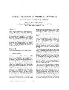
Fig. 1 shows and , the probabilities of selecting game A by Players 3 and 4, respectively. The figure also and , the probabilities of a reward for shows Player 3 selecting A or B, respectively. It can be seen that and as expected from , the theorem states Theorem 5.8. In the case and , which is shown in a). that The fact that game A, which requires cooperation, is less favorable to Player 3 than game B leads Player 3 to force the noncooperative result. However, in b), a particular run leads both players to favor cooperation and game A. The initial allows a few runs to actually demonstrate value accidental cooperation. This particular cooperative example disappears if we make the step length parameter even smaller, . Note that the use of learning automata in real say systems, say networks, implies that constants such as can have an effect on cooperation or noncooperation. Now consider noncoincident saddle points between game above and matrix
which has a saddle point at (2, 1). Fig. 2(a) shows the results and, again, and and the probabilities act accordingly. However, there are some plays of the game around where almost equals and, in Fig. 2(b), one particular run actually achieves an apparent equilibrium in with both players deciding to cooperate. To examine this result in more detail, Fig. 3 shows the , which goes to one, and , which goes strategies
ZHOU et al.: LEARNING IN MULTILEVEL GAMES
347
Fig. 1. Coincident saddle point games.
Fig. 2. Noncoincident saddle point games.
Fig. 3. Details of noncoincident saddle point games.
Fig. 4. Saddle point game versus nonsaddle point game.
to zero for the run in Fig. 2(a) and to one for the run in Fig. 2(b). Note that the absorbing state (1, 1) has the same payoff in game A and in game B, specifically 0.6. This means that Player 3 does not have a preference between game A and . Theorem 6.1 is still intact because it game B so precludes the game structure for saddle point ( ); however, these game structures may be encountered in real systems and cooperation could result. above, with a saddle point, Now consider game matrix and the following game matrix which does not have a saddle
point
Fig. 4 shows oscillations in the and strategies ). Note that games of a single run (in this case A and B are identical except for one value at (1, 2) which goes to zero to favors Player 4 in game B and, therefore, force this game. The oscillations are in this nonsaddle point game and have been observed in earlier work [5]. This is an
348
IEEE TRANSACTIONS ON SYSTEMS, MAN, AND CYBERNETICS—PART B: CYBERNETICS, VOL. 29, NO. 3, JUNE 1999
Fig. 5. Oscillations in noncoincident saddle point games.
example of players which can decide which game to play but cannot decide which strategy to favor within the context of the game. In the particular run above, the initialization favors of the time. However, an cooperation only initialization that more strongly favors cooperation will not exhibit oscillations as the agents reach equilibrium in the pure strategies of game A. Consider two game matrices with noncoincident saddle points
and
Various simulation runs show all four possible results of and going to zero or one. Fig. 5 shows one particular run and note that (350 000) almost with oscillations in reaches the absorbing state at zero, which other runs, not and shown, actually do reach. In this particular run, both go to one, hence cooperation. Note the interplay between and and . The oscillations in mean that sometimes game A is more favorable to Player 3 and sometimes game B, thus oscillates. The question arises as to is computed based the source of the oscillations in . Since and , there is an interplay on an expectation using and between the decisions about which game to play, , and which strategy to play within the game, and . In this particular run, oscillates between which , not shown, oscillates between which game to play as strategy to play. This illustrates the problem of multilevel decision making. Now consider two game matrices, neither of which has a saddle point:
and
Fig. 6. Oscillations in nonsaddle point games.
One particular run, see Fig. 6, results in a cooperative absorbing state and so did two other runs out of a total of 100 runs. The oscillations are more severe than in the previous case of noncoincident saddle points.
VIII. CONCLUSIONS In this study, we considered multilevel games and concentrated on the specific environment of zero-sum games with saddle points, decision making using the linear reward-inaction algorithm, and instantaneous exchange of information. The analysis has shown that noncooperation is typically the result in this specific environment. The reason for this is that, in zerosum games, one of the agents will find that game B is more to its advantage than game A, and any agent can unilaterally force game B to be played. The simulation results showed this typical noncooperative behavior as well as some rare cooperative behavior due to absorbing states and numerical simulation. However, more general environments can exhibit a variety of behaviors. Our companion study [2] considers nonzero-sum games, decision making using the linear reward-penalty algorithm, and delayed information exchange. The results show that, with very small penalties, chaotic behavior is possible. REFERENCES [1] E. Billard, “Stability of adaptive search in multi-level games under delayed information,” IEEE Trans. Syst., Man, Cybern. A, vol. 26, pp. 231–240, Mar. 1996. [2] E. Billard and S. Lakshmivarahan, “Learning in multi-level games with incomplete information—Part I,” IEEE Trans. Syst., Man, Cybern. B, this issue, pp. 329–339. [3] S. Lakshmivarahan, Learning Algorithms: Theory and Applications. New York: Springer-Verlag, 1981. [4] K. S. Narendra and M. A. L. Thathachar, Learning Automata: An Introduction. Englewood Cliffs, NJ: Prentice-Hall, 1989. [5] S. Lakshmivarahan and K. S. Narendra, “Learning algorithms for twoperson zero-sum stochastic games with incomplete information: A unified approach,” SIAM J. Contr. Optim., vol. 20, pp. 541–552, July 1982. [6] , “Learning algorithms for two-person zero-sum stochastic games with incomplete information,” Math. Oper. Res., vol. 6, pp. 379–386, Aug. 1981. [7] M. F. Norman, Markov Processes and Learning Models. New York: Academic, 1972. [8] , “On linear models with two absorbing barriers,” J. Math. Psychol., vol. 5, pp. 225–241, 1968.
ZHOU et al.: LEARNING IN MULTILEVEL GAMES
Jing Zhou received the B.S. degree in mathematics from Peking University, China, the M.S. degree in computer science, and the Ph.D. degree in mathematics from the University of Oklahoma, Norman. He is a Systems Engineer, Advanced Systems Division, Motorola Satellite Communications Group, Phoenix, AZ. Before he joined Motorola, he served as an Assistant Professor of Mathematics, Northwestern Oklahoma State University. His interests include optional control, parameter estimation, modeling and simulation, and learning algorithms.
349
Edward Billard, for a photograph and biography, see this issue, p. 339.
S. Lakshmivarahan, (M’81–SM’81–F’93) for a photograph and biography, see this issue, p. 339.