Abstractâ Robust target classification is an important feature of modern ..... [5] M.R. Inggs and A.D. Robinson, âShip Target Recognition Using Low. Resolution ...
http://www.dasp.ws/2005/Proceedings/szabo_dasp2004.pdf
Target Classification using High–Resolution Range Profiles Anthony P Szabo & Peter E Lawrence Defence Science & Technology Organisation, PO Box 1500, Edinburgh SA 5111. Abstract— Robust target classification is an important feature of modern sensors. In Defence applications, a robust target classification capability is crucial as a target may be prosecuted on the basis of the classification. Here target classification using high– resolution range (HRR) profiles will be discussed and a subset of the generic classification problem will be analysed. The wavelet transform is applied as a preprocessing technique to both denoising the data and locate the main scatterers in the profiles. The fidelity of this approach is demonstrated by comparing classification performance to a baseline that utilises the entire HRR profile as a feature vector. Wavelet based preprocessing is then applied to the scenario where contemporary HRR data is used to queue a third party sensor. In this case, training of the classifier is undertaken using data at one aspect angle and tested using data at a different aspect angle. Despite achieving some improvement through wavelet based preprocessing, classification performance is mixed when training and testing data sets are seperated by 30◦ in aspect.
I. I NTRODUCTION Robust target classification is an important feature of many modern senors, whether they be a medical imaging system [1] or collision avoidance radar [2]. In Defence applications, a robust target classification capability is particularly important as a target may be prosecuted on the basis of the classification. This requirement has driven a significant body of research investigating target classification algorithms for radars and electro– optical sensors (see e.g. [3] for a general description of the process and [4], [5], [6], [7], [8] for specific examples). Much of this previous work has focused on the generic problem of how to correctly classify a target when detected by a radar system. This is generally accomplished by comparing the signature of the target to a library of potential targets. Here we will consider a subset of this generic problem. We consider the case where the target has already been classified and contemporary data (e.g. feature vectors or parameters defining the trained classifier) are passed to a third party whose role is to find the correct target from a field of regard using its radar sensor. This case could be applied to the scenario where a targeting platform has detected, classified and designated a target and tasked a missile with a radio frequency (RF) seeker to find this target in a given region of interest. Framing the problem in this manner affects the way in which training and testing of the classifier is conducted. In this case, using sampling data from the same data set to both train and test the classifier is not a limitation of the analysis but rather an accurate representation of the scenario. Here a preprocessing technique using wavelet denoising and wavelet detection of transients or main scatterers in high– resolution range (HRR) profiles is described. The underlying
noise in the HRR profile data is removed by taking the continuous wavelet transform and applying a “soft–like” threshold to the wavelet coefficients on a scale–by–scale basis. The threshold is optimized in the least mean squared sense. Major scatterers in the denoised data are then detected by finding the wavelet modulus maxima (WMM). A natural consequence of this preprocessing is compaction of the feature vector, i.e. reduction of the feature vector from the entire HRR profile to the location and amplitude of a few main scatterers. We demonstrate that the resulting feature vector compaction does not significantly degrade the classification performance when using a support vector machine (SVM) classifier [9]. The robustness of using contemporary data to queue a third party is analysed by comparing the performance of the SVM classifier when trained using HRR data obtained from a given aspect and tested using HRR data from another aspect. In this case, scale and translational invariance are achieved by using a triangular kernal for the support vector machine [10]. For this scenario, we show that despite some improvements in classification performance through the application of wavelet base preprocessing, the SVM classifier demonstrated mixed performance when the training and testing data sets are seperated by 30◦ in aspect. The paper is organised as follows. The previous work on the application of the wavelet transform to target classification using HRR profiles is reviewed and summarised in Section II, along with a short description of the relevance of the current work. The application of the wavelet transform to denoising and detecting transients in HRR profiles is described in Sections III and IV, respectively. The technique adopted for wavelet denoising and feature extraction is summarised in Section V. The results are discussed in Section VI and the conclusions of this work are given in Section VII, along with suggestions for further work. II. P REVIOUS W ORK Several authors have described the application of the wavelet transform to the processing of HRR profiles (see e.g. [11], [12], [13]). Etemad and Challappa [11] consider the application of class separability–based tree–structured local basis design and feature selection to signal and image classification. They demonstrate their approach through the classification of one dimensional radar signals of five stationary targets and achieve good classification performance. Huether et al [12] discuss the application of the wavelet transform to denoising HRR profiles as a preprocessing step to classification. They consider noise in the abstract sense and aim to remove any signal that degrades
http://www.dasp.ws/2005/Proceedings/szabo_dasp2004.pdf the performance of the classifier. They apply a translational invariant wavelet denoising scheme to both real and synthetic HRR profiles, and optimized the denoising scheme with respect to several parameter including the choice of wavelet. They observed a significant improvement in classification performance when using this approach. Nelson et al [13] describes the application of the iterated wavelet transform to the selection of discriminant features in synthetic HRR profiles. They also treat the data abstractly and assume that any operation that improves the ability of the classifier to separate classes is desirable. They observe an improvement in the classifier performance through adopting this approach and show that, statistically, there is no advantage in choosing one family of wavelets over another. The approach adopted here differs from earlier work in several important respects. The continuous wavelet transform (CWT) is used instead of the discrete wavelet transform (DWT) so that optimal temporal resolution is achieved in the wavelet domain. The CWT also allows for translation–invariant denoising, whereas the DWT inherently cannot. Following denoising of the CWT, no attempt is made to reconstruct the profile prior to classification. This avoids Gibbs–like oscillations [14] appearing in the reconstructed signal due to the oscillatory nature of the analyzing wavelet. Instead, the main scatterers are located in the denoised CWT domain by locating and following the wavelet modulus maxima loci. Finally, a “soft–like” threshold is used here as it is closer to the theoretical optimum than the standard soft–threshold. III. WAVELET D ENOISING HRR profiles are denoised to remove the effects of background clutter and receiver noise, and to ensure that they do not give rise to spurious WMM. Denoising using the wavelet transform is possible because most of the energy contained in the wavelet transform of the noise is concentrate at lower scales and therefore amenable to thresholding [15]. Typically, wavelet–based denoising is performed with the discrete wavelet transform (DWT). Here we derive a denoising scheme using the CWT, inspired by Stein’s Unbiased Risk Estimation (SURE) [15]. Denoising will be performed on a scale–by–scale basis for the CWT coefficients. Generally, the background noise in the I– and Q–channels of a HRR profile will be the superposition of zero–mean iid Gaussian noise produced by the radar receiver, and a heavy–tailed non–Gaussian zero–mean noise component due to clutter. While the wavelet denoising methodology described here can be extended to include general background noise (see e.g. [16, §5]), here we assume that the additive noise in our profiles is zero–mean Gaussian. For a given digitized scale s , suppose that the sequence of CWT coefficients can be written as a vector X = (X1 , . . . , XM ) and that X ∼ N (θ, C), i.e. the coefficients are normally distributed, where θ = (θ1 , . . . , θM ) is a vector of coefficients representing the idealized signal that we wish to extract from an additive noise background, and C is a M × M covariance matrix with diagonal entries Cii = σi2 . Consider now an estimator θb of θ of the form θb = X + g(X) (1)
for some weakly–differentiable function g : RM → RM . We define a risk for this estimation as R(X) := E[kθb − θk2 ] =
M X
k=1
E[(θbk − θk )2 ],
(2)
where k · k is the standard Euclidean norm and E[ · ] is the expectation operator. In this case, we find that R(X) = E[tr(C) + kg(X)k2 + 2tr(C Dg(X))],
(3)
where tr( · ) is the trace function and Dg(X) := [∂gi (X)/∂Xj ]M×M is the Jacobian of g(X). Here, we will restrict ourselves to estimators based on point–wise thresholding, i.e. functions of the form gi (X) = ηT (Xi ) − Xi for some threshold T ≥ 0. In this case, as each gi is a function of Xi alone, the risk simplifies to R(X) =
M X
E[R(Xk , T )],
(4)
k=1
where R(Xk , T ) :=
σk2
2
+ gk (Xk ) +
2σk2
dgk (y) . dy y=Xk
(5)
We define an optimal threshold T ∗ as a minimizer of the risk R(X) with respect to T . As the parameters are seldomly known in practice it is not possible to compute T ∗ explicitly. Instead we choose an approximation Tb of T ∗ that minimizes an unbib ased estimator R(X; T ) of the risk R(X). Equation 4 gives us an unbiased estimator of the form b R(X; T) =
M X
R(Xk , T )
(6)
k=1
which is known as Stein’s Unbiased Risk Estimator (SURE). b The Stein principle is to minimize R(X; T ) with respect to T and take the minimizer [15], b Tb = arg min R(X; T) T >0
(7)
as a data–driven estimation of the optimal threshold T ∗ . Solving the minimization problem given by Equation 7 may be achieved by time–efficient gradient–based search methods, such as the conjugate–gradient method, so long as the functions gi are sufficiently differentiable. As standard “soft”– and “hard”–thresholding functions are not differentiable, we follow the methodology of Zhang [15] and use a “soft–like” threshold. This threshold is motivated by the differentiable sigmoid function and has demonstrated better denoising performance than the standard “hard”–limited thresholding techniques. This is because the threshold can be derived from a continuous rather than discrete set of values. Here we extend Zhang’s [15]“soft–like” thresholding function to accommodate complex valued data, yielding �� � � ( T x , |x| > T |x| − T − 2k+1 |x| (8) ηTk (x) := x 2k |x| , |x| ≤ T (2k+1)T 2k
http://www.dasp.ws/2005/Proceedings/szabo_dasp2004.pdf support, is n–times continuously differentiable and is the nth – derivative of a function whose integral is non–vanishing, then a function f (t) ∈ L1 [a, b] is singular, i.e. pointwise Lipschitz, at a point to ∈ [a, b] only if there is a sequence of WMM that converge toward to at finer scales [17, §6.2]. In addition if the analyzing wavelet is an nth –derivative of a Gaussian, Hummel [17, §6.2] has shown that the loci of WMM are never interrupted as the scale decreases. Hence by choice of a suitable wavelet we can detect transients in a signal by following the WMM to finer and finer scales. One such wavelet is the Marr or Mexican hat wavelet, which is the second derivative of a Gaussian function and given by � � � � t2 t2 (11) ψ(t) = 1 − 2 exp − 2 , 2σ σ
k=1 k=3 k=∞
k
ηT(x)
−T
0 x
T
k (x) applied to real–valued data x. Fig. 1. The “soft–like” threshold ηT
where k is a positive integer. This has been done to accomodate complex HRR data and will ensure that the phase of the complex–valued data is preserved by the thresholding process. Observe that ηTk becomes the standard “soft”–threshold function as k → ∞. This thresholding function is depicted in Figure 1 for different values of k. Note that Equation 5 remains unchanged, except that now the real– and imaginary–components of the function g must be included. In the case where the variances, σk2 , of the background noise at a given scale are unknown, we can replace them in Equation 5 with an estimate σ bk2 . In addition, if the real– and imaginary– components of the background noise each have homoscedastic covariance matrices, i.e. Cii = σ 2 , then we may use the median absolute deviation (MAD) estimate σ b of σ, via the formula σ b=
1 median (|X − median(X)|) , 0.6745
(9)
where X is the vector of associated CWT coefficients at the given scale. IV. T RANSIENT D ETECTION Given a complex–valued function ψ ∈ L1 (R) ∩ L2 (R) such R∞ 2 that the integral 0 (|Ψ(ω)| /ω) dω of the Fourier transform Ψ of ψ is a bounded and non–zero valued, the continuous wavelet transform (CWT) of a real–valued function f ∈ L2 (R) with respect to ψ is defined and denoted by [17] � � Z ∞ t−u 1 dt, (10) f (t)ψ ∗ Fψ (u, s) := √ s s −∞
where u ∈ R is the translation parameter, s > 0 the scale factor, and ∗ denotes complex conjugation. The CWT is the convolution, at a given scale s, of the function f (t) with the √ “time–frequency atom” ψ ((t − u)/s) / s, and measures the variation of f in the neighbourhood of u, whose size is proportional to s. We define a wavelet modulus maximum (WMM) as a point (uo , so ) ∈ R × R+ such that |Fψ (u, so )| has a strict local maximum at u = uo . If the analyzing wavelet ψ has compact
for σ > 0. While the Marr wavelet does not have compact support, it may be truncated due to its rapid decay beyond the points t = ±3σ. Here we use the Marr wavelet truncated on the interval [−5σ, 5σ]. We also use a standard deviation of σ = 1/2 in the analyzing wavelet in order to ensure little spread of the influence of a transient at the finest scale of the CWT. V. WAVELET D ENOISING & F EATURE E XTRACTION Here we will demonstrate the wavelet denoising and feature extraction technique used for the subsequent classification performance analysis by considering a sample HRR profile and following its progress through the preprocessing. An example of a typical raw HRR profile is shown in Figure 2. Shown are: (a) the I–component; (b) the Q–component; and (c) the absolute value; of the signal as a function of range bin. The data is dominated by a target region to the centre of the range window, flanked by noise regions on either side. The preprocessing method used here may be summarized as follows: (a) calculate the CWT of the HRR profile; (b) jointly denoise the CWT of the I– and Q–components of the profile; (c) locate the WMM and follow the connected loci down to the finest scale; and (d) remove outliers. Each of these steps is described in detail below. We calculate the CWT with respect to the truncated Marr analyzing wavelet by performing a discrete convolution implemented via the fast fourier transform (FFT). We seperately calculate the CWT for both the I– and Q–components of the HRR profiles. We choose the scale factor interval to range from the sampling rate of the sampled signal to a value where only 3% of convolution edge–effects are present, again sampled at the same rate as the signal. We denoise the CWT for both the I– and Q–components at each scale according to the SURE principle using our “soft– like” threshold. As the thresholding function, ηTk (x), is twice continuously differentiable for T > 0 with respect to both variables x and T for any positive integer k , we solve the optimization problem defined by Equation 7 by a gradient–based search algorithm. Here we used the conjugate–gradient iterative method with k = 3. We form the modulus of the resulting complex–valued map and locate the associated WMM by finding the values that are strictly greater than both left and right adjacent values. This is done on a scale–by–scale basis and the boundary points are
http://www.dasp.ws/2005/Proceedings/szabo_dasp2004.pdf (a): I−Component 20 10 0 −10
Normalized Amplitude
−20
50
100
150
200
250
100
150
200
250
150
200
250
(b): Q−Component
20 10 0 −10 −20
50
(c): Absolute Value
25 20 15 10 5 0
50
100
Range Bin
Fig. 2. An example of a raw HRR profile. Aspect of 30◦ .
(a): Transients Located in Raw Profile
20 10 0 −10
Normalized Amplitude
−20
100
150
200
250
50
100
150
200
250
50
100
150
200
250
50
(b): Transients Located in Denoised Profile
20 10 0 −10 −20
(c): Transients Located following Outlier Removal 20 10 0 −10 −20
Range Bin
Fig. 3. An example of a denoised and feature extracted I–component.
ignored. These values are clustered between adjacent scales according to a single–linkage nearest–neighbour principle in order to form the WMM loci. Each WMM loci is traced from the largest to finest scale, and the location of each locus along the time–axis at this finest scale is then recorded as the position of a transient in the original signal. We remove outliers by segmenting the transients into three regions, a central target region and two flanking noise regions. This is implemented using the K–means clustering methos with the Mahalanobis metric [18] An example of a HRR profile after each step is shown in Figure 3. Shown are: (a) the feature vector without preprocessing; (b) the feature vector when the profile is wavelet denoised; and (c) the denoised feature vector when outliers are removed. In each case only the I–component has been shown for clarity. VI. R ESULTS Here we use real HRR profiles collected at X–Band by an airborne radar system. HRR data on four surface targets, here
designated C1 , C2 , C3 and C4 , has been used in this analysis. The targets all represent different target classes. The data was collected at aspect angles of 0◦ (end on), 30◦ and 60◦ , with the aspect varying by about a degree over the data set in each case. Unfortunately, the data set is very small (only 20 HRR profiles for each target at each aspect) and the consequences of this for our analysis are discussed below. Here we have used a Support Vector Machine to classify our targets. This has been implemented via the Matlab Ohio State University (OSU) SVM toolbox obtained freely from http://www.ece.osu.edu/∼maj/osu svm/. Further information on this classifier may be found at this site. To gauge the baseline performance of the classifier, half of the HRR data for the four targets at an aspect of 30◦ was randomly selected and used to train the SVM classifier. Here the amplitude of the entire HRR profile is used as the feature vector. Note that no translation or scale transformations are required for the data as the targets are stationary within the range window and represent a narrow range of aspect angles. The other half of the data at the same aspect was then used to test the classifier. The results are shown in Table I in the form of a confusion matrix (central columns marked 30◦ ). In this case we can see that the classifier correctly classifies all four targets. The result when the data is preprocessed by wavelet denoising and the feature extracted is shown in Table II (central columns marked 30◦ ). In this case, the feature vectors only contain the amplitude and location of the main scatterers present in the data. The classification performance is largely unchanged, indicating that the compacted feature vector adequately represents the target for the purposes of classification. The small data set means that there is a 10% error in the values on the confusion matrix and hence the mis–classification of target C1 10% of the time is not statistically significant. To gauage the feasibility of using contemporary data to cue classification by a third party, the classifier is trained with data at an aspect of 30◦ and then tested with data from another aspect, i.e. 0◦ or 60◦ . In this case, the data needs to be made scale and translational invariant as the apparent size and location of the target in the range window changes from aspect to aspect. Scale and translational invariance may be achieved by taking the Fourier modified direct Mellin transform (FMDMT) [19] prior to classification. However, this transform is known to degrade the interclass separability in classification problems [7] and so we instead incorporate scale and translational invariance into our SVM classifier by using a triangular kernel [10]. As a baseline, the classification results when the entire HRR profile is used as feature vector are shown in Table I (columns marked 0◦ and 60◦ ). Here the classifier is trained using all of the 30◦ aspect data and tested using all the 0◦ and 60◦ data. In this case, we can see that the classifier correctly classified targets C1 and C3 most of the time and mis–classifies targets C2 and C4 most of the time. The results when the data is wavelet–denoised and feature extracted are shown in Table II. In this case, we see mixed classification results. Classification of targets C1 and C3 is improved through the application of wavelet based preprocessing, yielding correct classifications 95% and 100% of the time, respectively. However, targets C2 and C4 are classified poorly,
http://www.dasp.ws/2005/Proceedings/szabo_dasp2004.pdf TABLE I BASELINE R ESULTS .
30◦
0◦
C1 C2 C3 C4
C1 90 0 0 0
C3 0 100 100 100
C2 10 0 0 0
C4 0 0 0 0
C1 100 0 0 0
C3 0 0 100 0
C2 0 100 0 0
C4 0 0 0 100
C1 95 0 0 0
60◦ C3 C2 0 0 10 25 100 0 0 50
C4 5 65 0 50
TABLE II WAVELET P REPROCESSED R ESULTS .
0◦
C1 C2 C3 C4
C1 95 0 0 0
C2 0 0 0 0
C3 0 100 100 100
C4 5 0 0 0
C1 90 0 0 0
30◦ C3 C2 0 10 0 100 100 0 0 0
although the classification of C2 is improved somewhat through the use of wavelet based proprocessing. VII. C ONCLUSIONS & F URTHER W ORK The wavelet denoising and feature extraction scheme described here is an effective means of compacting feature vector data, without compromising classification performance. This may provide significant benefit where large databases of target classification data exist, allowing the data to be stored more efficiently. Alternatively in applications where the feature vector needs to be transmitted via datalink, compaction may significantly reduce the bandwidth required for transmission. This approach may also provide benefits where contemporary data is used to queue target classification by a third party, e.g. where an RF missile is tasked by a targeting platform to find a given target. However, the data set used here isn’t large enough to draw strong conclusions, although there are some indications of improved classification performance. The limited nature of the analysis presented here also makes it difficult to draw conclusions about the feasibility of queued classification by a third party. Some targets are correctly classified virtually all of the time despite training and testing data sets being seperated by 30◦ in aspect. Unfortunately, other targets are mis– classified almost as often. Further work will expand the analysis through the use of a larger data set, including more HRR profiles at each aspect and a finer graduation in the range of aspects. The effectiveness of using wavelet based preprocessing when using low signal–to– noise HRR data will also be investigated. ACKNOWLEDGEMENTS The authors would like to thank Dr Brett Haywood for providing the data used in the analysis presented here. The authors would also like to thank Dr Andrew Shaw and Dr Danny Gibbins for helpful comments on the original manuscript. R EFERENCES [1] A. Mojsilovic and J. Gomes, “Semantic Based Categorisation, Browsing and Retrieval in Medical image Databases”, Proceedings of International Conference on Image Processing, vol. III, pp. 145–148, 2002.
60◦
C4 0 0 0 100
C1 100 0 0 25
C2 0 75 0 60
C3 0 5 100 0
C4 0 20 0 15
[2] M.R. Nicholls, “Millimetre Wave Collision Avoidance Radars”, IEE Colloquium on Millimetre–Wave Radar, 23 May 1990, pp. 3/1–3/7, 1990. [3] N.F. Ezquerra, “Target Recognition Considerations” in Principles of Modern Radar, edited by J.L. Eaves and E.K. Reedy, Van Nostrand Reinhold Company Inc., New York, pp. 646–677, 1987. [4] A. Zyweck and R.E. Bogner, “Radar Target Classification of Commercial Aircraft”, IEEE Trans. Aero. Elec. Sys., vol. 32(2), pp. 598–606, April 1996. [5] M.R. Inggs and A.D. Robinson, “Ship Target Recognition Using Low Resolution Radar and Neural Networks”, IEEE Trans. Aero. Elec. Sys., vol. 35(2), pp. 386–393, April 1999. [6] R.A. Mitchell and J.J. Westerkamp, “Robust Statistical Feature Based Aircraft Identification”, IEEE Trans. Aero. Elec. Sys., vol. 35(3), pp. 1077–1094, July 1999. [7] S. Slomka, D. Gibbins, D. Gray and B. Haywood, “Features for High Resolution Radar Range Profile based Ship Classification”, Proceedings of the Fifth International Symposium on Signal Processing and Its Applications, ISSPA ’99, 22–25 Aug. 1999, vol. 1, pp.:329–332, 1999. [8] S.P. Jacobs and J.A. O’Sullivan, “Automatic Target Recognition Using Sequences of High Resolution Radar Range–Profiles”, IEEE Trans. Aero. Elec. Sys., vol. 36(2), pp. 364–382, April 2000. [9] C. Junli and J. Licheng, “Classification mechanism of support vector machines”, 5th International Conference on Signal Processing Proceedings, WCCC-ICSP 2000. , vol. 3, pp. 21-25, August 2000. [10] F. Fleuret and H. Sahbi, “Scale Invariance of Support Vector Machines based on the Triangular Kernel”, (in ICCV2003 workshop SCTV 2003 on Statistical and Computational Theories of Vision). [11] K. Etemad and R. Challappa, “Separability–Based Multiscale Basis Selection and Feature Extraction for Signal and Image Classification”, IEEE Trans. Image Proc., vol. 7(10), pp. 1453–1465, October 1998. [12] B.M. Huether, S.C. Gustafson and R.P. Broussard, “Wavelet Preprocessing for High Range Resolution Radar Classification”, IEEE Trans. Aero. Elec. Sys., vol. 37(4), pp. 1321–1332, October 2001. [13] D.E. Nelson, J.A. Starzyk and D.D. Ensley, “Iterated Wavelet Transformation and Signal Discrimination for HRR Radar Target Recognition”, IEEE Trans. Sys. Man Cyb., Part A, vol. 33(1), pp. 52–57, January 2003. [14] S.D. Durand and J. Froment, “Artifact Free Signal Denoising with Wavelets”, Proceedings of 2001 IEEE International Conference on Acoustics, Speech, and Signal Processing, ICASSP ’01, vol. 6, pp. 3685– 3688, 7–11 May 2001. [15] X. Zhang and M.D. Desai, “Adaptive Denoising Based on SURE Risk”, IEEE Sig. Proc. Lett., vol. 5, no. 10, pp. 265–267, October 1998. [16] R. Averkamp and C. Houdr´e, “Wavelet thresholding for non (necessarily) Gaussian noise: Functionality”. Preprint, 1999. [17] S. Mallat, “A Wavelet Tour of Signal Processing”, Academic Press, SanDiego, CA. 1999. [18] A. Webb, “Statistical Pattern Recognition”, Arnold Publishers, New York, 1999. [19] P.E. Zwicke and I. Kiss Jr., “A New Implementation of the Mellin Transform and its Applications to Radar Classification of Ships”, IEEE Trans. Patt. Anal. Mach. Intel., vol. PAMI-5, no. 2, pp. 191–199 March 1983.