Target Classification with Simple Infrared Sensors Using Artificial Neural Networks Tayfun Aytac¸ ¨ ˙ TUBITAK-UEKAE/˙ILTAREN S¸ehit Yzb. ˙Ilhan Tan Kıs¸lası ¨ Umitk¨ oy, TR-06800 Ankara, Turkey
Billur Barshan Department of Electrical and Electronics Engineering, Bilkent University Bilkent, TR-06800 Ankara, Turkey
[email protected]
[email protected]
Abstract— This study investigates the use of low-cost infrared (IR) sensors for the determination of geometry and surface properties of commonly encountered features or targets in indoor environments, such as planes, corners, edges, and cylinders using artificial neural networks (ANNs). The intensity measurements obtained from such sensors are highly dependent on the location, geometry, and surface properties of the reflecting target in a way which cannot be represented by a simple analytical relationship, therefore complicating the localization and classification process. We propose the use of angular intensity scans and feature vectors obtained by modeling of angular intensity scans and present two different neural network based approaches in order to classify the geometry and/or the surface type of the targets. In the first case, where planes, 90◦ corners, and 90◦ edges covered with aluminum, white cloth, and Styrofoam packaging material are differentiated, an average correct classification rate of 78% of both geometry and surface over all target types is achieved. In the second case, where planes, 90◦ edges, and cylinders covered with different surface materials are differentiated, an average correct classification rate of 99.5% is achieved. The method demonstrated shows that ANNs can be used to extract substantially more information than IR sensors are commonly employed for.
Application areas of IR sensing include robotics and automation, process control, remote sensing, and safety and security systems. More specifically, they have been used in simple object and proximity detection, counting, distance and depth monitoring, floor sensing, position control, obstacle/collision avoidance, and machine vision systems. IR sensors are used in door detection, mapping of openings in walls [8], as well as monitoring doors/windows of buildings and vehicles, and light curtains for protecting an area. In [9], IR sensors are employed to locate edges of doorways in a complementary manner with sonar sensors. Other researchers have also dealt with the fusion of information from IR and sonar sensors [10], [11], [12]. In [13], the properties of a planar surface at a known distance have been determined using the Phong illumination model, and using this information, the IR sensor employed has been modeled as an accurate range finder for surfaces at short ranges. Reference [14] also deals with determining the range of a planar surface. By incorporating the optimal amount of additive noise in the IR range measurement system, the authors were able to improve the system sensitivity and extend the operating range of the system. In [15], an IR sensor-based system which can measure distances up to 1 m is described. References [16], [17], [18] deal with optical determination of depth information. In [19], simulation and evaluation of the recognition abilities of active IR sensor arrays is considered for autonomous systems using a raytracing approach. In [20], the authors developed a novel range estimation technique which is independent of surface type since it is based on the position of the maximum intensity value instead of surface-dependent absolute intensity values. An intelligent feature of the system is that its operating range is made adaptive based on the maximum intensity of the detected signal. Our earlier works on IR based target classification include rule-based target classification explained in [21], templatebased geometry and surface classification and localization proposed in [22], [23], [24], parametric surface classification [25], and statistical pattern recognition based target classification [26].
I. INTRODUCTION ANNs have been widely used in areas such as target detection and classification [1], speech processing [2], system identification [3], control theory [4], medical applications [5], and character recognition [6]. Neural networks have been employed efficiently as pattern classifiers in numerous applications [7]. These classifiers are non-parametric and make weaker assumptions on the shape of the underlying distributions of input data than traditional statistical classifiers. Therefore, they can prove more robust when the underlying statistics are unknown or the data are generated by a nonlinear system. Due to single intensity readings not providing much information about the target properties, recognition capabilities of IR sensors have been underestimated and underused in most of the earlier work. The aim of this study is to maximally realize the potential of these simple sensors so that they can be used in more complicated tasks such as classification, recognition, clustering, docking, perception of the environment and surroundings, and map building. For this purpose, we employ ANNs with different inputs to classify targets with different geometries, different surface properties, and the combination of the two.
II. IR S ENSOR AND THE E XPERIMENTAL S ETUP The IR sensor [27] used in this study consists of an emitter and detector and works with 20–28 V DC input
978-1-4244-2881-6/08/$25.00 ©2008 IEEE
Authorized licensed use limited to: Bu hizmeti TUBITAK EKUAL kapsaminda ULAKBIM saglar. Downloaded on November 13, 2009 at 09:47 from IEEE Xplore. Restrictions apply.
(a)
(b)
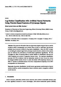
Fig. 1. (a) The IR sensor and (b) the experimental setup used in this study.
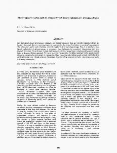
voltage, and provides an analog output voltage proportional to the measured intensity reflected off the target. The detector window is covered with an IR filter to minimize the effect of ambient light on the intensity measurements. Indeed, when the emitter is turned off, the detector reading is essentially zero. The sensitivity of the device can be adjusted with a potentiometer to set the operating range of the system. The IR sensor [see Fig. 1(a)] is mounted on a 12 inch rotary table [28] to obtain angular intensity scans from these targets. A photograph of the experimental setup can be seen in Fig. 1(b). The target primitives employed in this study are a plane, a 90◦ corner, a 90◦ edge, and a cylinder. The horizontal extent of all targets are large enough that they can be considered infinite and thus edge effects need not be considered. They are covered with different materials of different surface properties, each with a height of 120 cm. III. TARGET C LASSIFICATION U SING ANN S ANNs are employed to identify and resolve parameter relations embedded in the characteristics of IR intensity scans acquired from target types of different geometry, possibly with different surface properties, for their classification in a robust manner. Two different ANNs are employed for target classification. In the first case, angular intensity scans are used as inputs [29]. In the second case, angular intensity scans obtained from planes, edges, and cylinders of different surface properties are physically modeled and model parameters are used as inputs to the ANN [26]. A. ANN Classifiers Using Angular Intensity Scans The targets employed in this part of the study are plane, corner, and edge, covered with aluminum, white cloth, and Styrofoam packaging material. Reference data sets are collected for each geometry-surface combination with 2.5 cm distance increments, from their nearest to their maximum observable ranges, at θ = 0◦ . The resulting reference scans are shown in Fig. 2. Note that these scans are the original scans, not their downsampled versions used as training inputs to the ANN. The training set consists of 147 sample scans, 60 of which correspond to planes, 49 of which correspond to corners, and 38 of which correspond to edges. The number of scans for each geometry is different. This is because the targets have different reflective properties and each target is detectable over a different distance interval determined by its geometry and surface properties. We have chosen to acquire the training scans in a uniformly distributed fashion
over the detectable range for each target. Training is done by the Levenberg-Marquardt (LM) algorithm. The input weights are initialized randomly. The ANN resulting in the highest correct classification rate on the training and test sets has 10 hidden-layer neurons in fully connected form. We test the ANN with IR data acquired by situating targets at randomly selected distances r and azimuth angles θ and collecting a total of 194 test scans, 82 of which are from planes, 64 from corners, and 48 from edges. The targets are randomly located at azimuth angles varying from −45◦ to 45◦ from their nearest to their maximum observable ranges. (Note that the test scans are collected for random target positions and orientations whereas the training set was collected for targets at equally-spaced ranges at θ = 0◦ .) When a test scan is obtained, first, the azimuth of the target is estimated using the center-of-gravity (COG) and/or the maximum intensity of the scans. The test scans are shifted by the azimuth estimate, then downsampled by 10, and the resulting scan is used as input to the ANN. The classification results for the COG case are shown in Table I in parentheses, where an overall correct differentiation rate of 94.3% is achieved. Corners are always correctly identified and not confused with the other target types due to the special nature of their scans. Planes are confused with edges at six instances out of 82 and similarly, edges are confused with planes in five cases out of 48. Secondly, to observe the effect of the azimuth estimation method, we used the maximum values of the unsaturated intensity scans. The overall correct differentiation rate in this case is 96.4% (given outside the parentheses in Table I), which is better than that obtained using COG, due to the improvement in the classification of edges. Except for seven planar test scans, all planes are correctly differentiated. Six of the seven incorrectly classified planar test targets are covered with aluminum, whose intensity scans are saturated. At the next step, Optimal Brain Surgeon technique [30] is implemented for finding the optimal network structure. The plot of training and test errors with respect to the number of weights left after pruning is shown in Fig. 3. In this figure, the errors evolve from right to left. The minimum error is obtained on the test set when 263 weights are used. The eliminated weights are set to zero. As the number of weights is decreased beyond 263, both the training and test errors increase rapidly due to the elimination of too many weights. If 263 weights are kept, the corresponding number of hiddenlayer neurons is still 10. Using the weights resulting in the smallest test error, we retrained the network again with the LM algorithm but with zero weight decay factor. The ANN converges in seven iterations to an error of 0.00033. The differentiation results for the optimized network are given in Table II. An overall correct differentiation rate of 99.0% is achieved. Therefore, apart from optimizing the structure of the ANN, pruning the network resulted in improved geometry differentiation. We consider differentiating the surface types of the targets assuming their geometries are correctly identified previously. The same network structure and the same procedure used in geometry differentiation is employed in surface type
Authorized licensed use limited to: Bu hizmeti TUBITAK EKUAL kapsaminda ULAKBIM saglar. Downloaded on November 13, 2009 at 09:47 from IEEE Xplore. Restrictions apply.
12
10
10
10
8
8
8
6
INTENSITY (V)
12
INTENSITY (V)
INTENSITY (V)
12
6
4
4
4
2
2
2
0 −90 −75 −60 −45 −30 −15
0
15
30
45
60
75
0 −90 −75 −60 −45 −30 −15
90
SCAN ANGLE (deg)
15
30
45
60
75
0 −90 −75 −60 −45 −30 −15
90
12
10
10
10
8
8
8 INTENSITY (V)
12
6
4
4
2
2
2
0
20
40
60
80 100 120
0 −120−100 −80 −60 −40 −20
SCAN ANGLE (deg)
0
20
40
60
80 100 120
0 −120−100 −80 −60 −40 −20
SCAN ANGLE (deg)
(d)
10
10
10
8
8
8 INTENSITY (V)
12
INTENSITY (V)
12
6
4
4
2
2
2
0
15
30
45
60
75
90
0 −90 −75 −60 −45 −30 −15
0
15
SCAN ANGLE (deg)
(g)
(h)
75
90
0
20
40
60
80 100 120
30
45
60
6
4
SCAN ANGLE (deg)
60
(f)
12
0 −90 −75 −60 −45 −30 −15
45
SCAN ANGLE (deg)
(e)
6
30
6
4
0 −120−100 −80 −60 −40 −20
15
(c)
12
6
0
SCAN ANGLE (deg)
(b)
INTENSITY (V)
INTENSITY (V)
0
SCAN ANGLE (deg)
(a)
INTENSITY (V)
6
30
45
60
75
90
0 −90 −75 −60 −45 −30 −15
0
15
75
90
SCAN ANGLE (deg)
(i)
Fig. 2. Intensity scans for targets (first row, plane; second row, corner; third row, edge) covered with different surfaces (first column, aluminum; second column, white cloth; third column, Styrofoam) at different distances.
classification.
B. ANN Classifiers Using Feature Vectors
For each geometry, all surface types are correctly differentiated in the training set. In Table III, the confusion matrix for the three geometries and surfaces is given. For planes, an average correct differentiation rate of 80.5% is achieved. Planes covered with aluminum are correctly classified with 100% correct differentiation rate. The surface types of the corners are correctly classified with a rate of 85.9%. All corners covered with aluminum are correctly differentiated due to their distinctive features. Worst classification rate (64.6%) is achieved for edges due to their narrower basewidths. Edges covered with white cloth are not confused with Styrofoam packaging material. However, edges covered with Styrofoam are incorrectly classified as edges covered with white cloth with a rate of 72.2%. An overall correct differentiation rate of 78.4% is achieved for all surfaces.
In this part of the study, only the reflection coefficients obtained by modeling the IR intensity scans are used as input to the ANN in the classification process, instead of using the angular IR intensity scans as in the previous section. The geometries considered are plane, edge, and cylinder made of unpolished oak wood. The surfaces are either left uncovered (plain wood) or alternatively covered with Styrofoam packaging material, white and black cloth, and white, brown, and violet paper (matte). Reference intensity scans are collected for each target type by positioning the surfaces over their observable ranges with 2.5 cm distance increments, at θ = 0◦ . Sample reference scans for wooden targets are shown in Fig. 4 using dotted lines (see [26] for all reference scans). These intensity scans have been modeled by approximating the surfaces as ideal Lambertian (or diffusely reflecting) surfaces since all of the
Authorized licensed use limited to: Bu hizmeti TUBITAK EKUAL kapsaminda ULAKBIM saglar. Downloaded on November 13, 2009 at 09:47 from IEEE Xplore. Restrictions apply.
TABLE III C ONFUSION MATRIX FOR THREE GEOMETRIES AND THREE SURFACE TYPES . (AL: ALUMINUM , WC: WHITE CLOTH , ST: S TYROFOAM .)
1.4 training error test error
1.2 1
error
0.8
a c t u a l
0.6 0.4 0.2
P
AL WC ST
C
AL WC ST
E
AL WC ST
0 −0.2 0
200
400
600
800
1000
1200
1400
1600
number of weights
Fig. 3.
Test and training errors while pruning the ANN with OBS.
surface materials involved were matte. The received return signal intensity is proportional to the detector area and is inversely proportional to the square of the distance to the surface and is modeled with three parameters as I=
C0 cos(αC1 ) 2 [ cosz α +R( cos1 α −1)]
(1)
In Eqn. (1), the product of the intensity of the light emitted, the area of the detector, and the reflection coefficient of the surface is lumped into the constant C0 , and C1 is an additional coefficient to compensate for the change in the basewidth of the intensity scans with respect to distance (Fig. 4). A similar dependence on C1 is used in sensor modeling in [31]. The z is the horizontal distance between the rotary platform and the target. The denominator of I is the square of the distance d between the IR sensor and the z+R surface. From the geometry of setup, d + R = cos α , from z 1 which we obtain d as cos α + R( cos α − 1), where R is the TABLE I C ONFUSION MATRIX FOR ANN BEFORE O PTIMAL B RAIN S URGEON : RESULTS ARE OUTSIDE ( INSIDE ) THE PARENTHESES FOR MAXIMUM INTENSITY (COG) BASED AZIMUTH ESTIMATION . (P: P LANE , C: C ORNER , E: E DGE ) target
differentiation result P C E 75(76) –(–) 7(6) –(–) 64(64) –(–) –(5) –(–) 48(43) 75(81) 64(64) 55(49)
P C E total
total 82(82) 64(64) 48(48) 194(194)
TABLE II C ONFUSION MATRIX FOR ANN AFTER O PTIMAL B RAIN S URGEON . target P C E total
differentiation result P C E 80 – 2 – 64 – – – 48 80 64 50
total 82 64 48 194
d e t e c t e d P AL WC ST 24 – – – 23 6 – 9 19 C AL WC ST 22 – – – 14 8 – 1 19 E AL WC ST 8 – – – 19 – – 13 4
U – – 1 – – – 2 1 1
radius of the rotary platform and α is the angle between the IR sensor and the horizontal. Using the model represented by Eqn. (1), parameterized curves have been fitted to the reference intensity scans by employing a nonlinear least-squares technique based on a model-trust region method provided by MATLABTM [32]. Resulting sample curves for wooden targets are shown in Fig. 4 in solid lines. For the reference scans, z is not taken as a parameter since the distance between the surface and the IR sensing unit is already known. The initial guesses of the parameters must be made cleverly so that the algorithm does not converge to local minima and curve fitting is achieved in a smaller number of iterations. The initial guess for C0 is made by evaluating I at α = 0◦ , and corresponds to the product of I with z 2 . Similarly, the initial guess for C1 is made by evaluating C1 from Eqn. (1) at a known angle α different than zero, with the initial guess of C0 and the known value of z. While curve fitting, C0 value is allowed to vary between ± 2000 of its initial guess and C1 is restricted to be positive. The variations of C0 , C1 , and z with respect to the maximum intensity of the reference scans are shown in Fig. 5. As the distance d decreases, the maximum intensity increases and C0 first increases then decreases but C1 and z both decrease, as expected from the model represented by Eqn. (1). After nonlinear curve fitting to the observed scan, we get three parameters C0 , C1 , and z. We begin by constructing two alternative feature vector representations based on the parametric representation of the IR scans. The feature vector x is a 2×1 column vector comprised of the [C1 , Imax ]T pair, illustrated in Figs. 5 (a) and (b), respectively. Feed-forward ANNs trained with back-propagation (BP) and LM algorithms, and a linear perceptron (LP) are used as classifiers. The feed-forward ANN has one hidden layer with four neurons. The number of neurons in the input layer is two (since the feature vector consists of two parameters) and the number of neurons in the output layer is three. LP is the simplest type of ANN, used for classification of two classes that are linearly separable. LP consists of a single neuron with adjustable input weights and a threshold value [33]. If the number of classes is greater than two,
Authorized licensed use limited to: Bu hizmeti TUBITAK EKUAL kapsaminda ULAKBIM saglar. Downloaded on November 13, 2009 at 09:47 from IEEE Xplore. Restrictions apply.
10
10
8
8
8
6
intensity (V)
12
10
intensity (V)
12
intensity (V)
12
6
6
4
4
4
2
2
2
0 −50
−40
−30
−20
−10
0
10
20
30
40
50
scan angle (deg)
0 −60
−40
−20
(a) Plane Fig. 4.
0 scan angle (deg)
20
40
0 −50
60
−40
−30
(b) Edge
−20
−10 0 10 scan angle (deg)
20
30
40
50
(c) Cylinder
Intensity scans for wooden targets at different distances. Solid lines indicate the model fit and the dotted lines indicate the actual data.
20
55
12000
wood Styrofoam white cloth black cloth white paper brown paper violet paper
18 16 14
C0 coefficient
8000
4000
45
40
12 10
1
6000
wood Styrofoam white cloth black cloth white paper brown paper violet paper
50
z (cm)
C coefficient
10000
wood Styrofoam white cloth black cloth white paper brown paper violet paper
35
8 30
6 25
4 2000 20
2 0 0
2
4
6
Imax (V)
8
10
12
0 0
2
4
6
I
max
(a)
8
10
12
(V)
15
0
2
4
(b)
6
Imax (V)
8
10
12
(c)
Fig. 5. Variation of the parameters (a) C0 , (b) C1 , and (c) z with respect to maximum intensity (dashed, solid, and dotted lines are for planes, edges, and cylinders, respectively). TABLE IV
TABLE V
G EOMETRY CONFUSION MATRIX : ANN TRAINED WITH BP.
G EOMETRY CONFUSION MATRIX : ANN TRAINED WITH LM.
geometry P E CY total
differentiation result P E CY 70(84) 0(0) 0(0) 0(0) 52(40) 3(3) 0(0) 0(0) 50(84) 70(84) 52(40) 53(87)
total 70(84) 55(43) 50(84) 175(211)
LPs are used in parallel. One perceptron is used for each output. The maximum number of epochs is chosen as 1000. The weights are initialized randomly and the learning rate is chosen as 0.1. MATLABTM Neural Network Toolbox is used for the implementation. The correct differentiation rates using the BP algorithm are given in Table IV. Differentiation rates of 98.3% and 98.6% are achieved for the training and test sets, respectively. When training is done by LM, the same correct differentiation rate is obtained on the training set (see Table V). However, this classifier is better than the BP method in the tests, where only one edge target is misclassified as a cylinder, resulting in a correct differentiation rate of 99.5%. The results for the LP classifier are given in Table VI. As expected from the distribution of the parameters, because the classes are not linearly separable, lower correct differentiation rates of 77.7% and 76.3% are achieved on the training and test sets, respectively. IV. C ONCLUSIONS In this study, we propose two different ANNs for classification of the geometry and/or the surface type of the
geometry P E CY total
differentiation result P E CY 70(84) 0(0) 0(0) 0(0) 52(42) 3(1) 0(0) 0(0) 50(84) 70(84) 52(42) 53(85)
total 70(84) 55(43) 50(84) 175(211)
TABLE VI G EOMETRY CONFUSION MATRIX : LP. geometry P E CY total
differentiation result P E CY 70(84) 0(0) 0(0) 0(0) 45(32) 10(11) 0(0) 29(39) 21(45) 70(84) 74(71) 31(56)
total 70(84) 55(43) 50(84) 175(211)
targets. In the first case, an optimal neural network structure is proposed for improved target classification with IR sensor. The input signals are the intensity scans obtained by rotating a point sensor from different targets. The intensity scans are preprocessed by downsampling to decrease the computational complexity of the network. The training algorithms employed are BP and LM. The networks trained with LM are pruned Optimal Brain Surgeon technique for the optimal network structure. Pruning also results in improved classification. A modular approach is adopted where first the geometry of the targets is determined and later on the surface type. Geometry type of the targets is classified with 99% accuracy. Only two planes are incorrectly classified as
Authorized licensed use limited to: Bu hizmeti TUBITAK EKUAL kapsaminda ULAKBIM saglar. Downloaded on November 13, 2009 at 09:47 from IEEE Xplore. Restrictions apply.
edges. For the surface type determination, an overall correct differentiation rate of 78.4% is achieved for all surfaces. In the second case, we construct feature vectors based on the parameters of angular IR intensity scans from different targets to determine their geometry and/or surface type. An average correct classification rate of 99.5% is achieved. Surface differentiation was not as successful as geometry differentiation due to the similar characteristics of the intensity scans of different surface types for the different geometries. The results indicate that the geometrical properties of the targets are more distinctive than their surface properties, and surface determination is the limiting factor in differentiation. Given the attractive performance-for-cost of IR-based systems, we believe that the results of this study will be useful for engineers designing or implementing IR systems and researchers investigating algorithms and performance evaluation of such systems. While we have concentrated on IR sensing, the techniques evaluated and compared in this paper may be useful for other sensing modalities and environments where the objects are characterized by complex signatures and the information from a multiplicity of partial viewpoints must be combined and resolved. ACKNOWLEDGMENT This work is supported in part by The Scientific and Tech¨ ˙ITAK) under nological Research Council of Turkey (TUB grant number EEEAG-105E065. R EFERENCES [1] B. C. Bai and N. H. Farhat, “Learning networks for extrapolation and radar target identification,” Neural Networks, vol. 5, pp. 507–529, May/June 1992. [2] M. Cohen, H. Franco, N. Morgan, D. Rumelhart, and V. Abrash, “Context-dependent multiple distribution phonetic modelling with MLPs,” in Advances in Neural Information Processing Systems (S. J. Hanson, J. D. Cowan, and C. L. Giles, ed.), pp. 649–657, San Mateo, CA: Morgan Kaufmann, 1993. [3] K. S. Narendra and K. Parthasarathy, “Gradient methods for the optimization of dynamic systems containing neural networks,” IEEE Trans. Neural Networks, vol. 2, pp. 252–262, Mar. 1991. [4] M. I. Jordan and R. A. Jacobs, “Learning to control an unstable system with forward modeling,” in Advances in Neural Information Processing Systems 2 (D. S. Touretzky, ed.), pp. 324–331, San Mateo, CA: Morgan Kaufmann, 1990. [5] M. Galicki, H. Witte, J. D¨orschel, M. Eiselt, and G. Griessbach, “Common optimization of adaptive processing units and a neural network during the learning period: application in EEG pattern recognition,” Neural Networks, vol. 10, pp. 1153–1163, Aug. 1997. [6] Y. LeCun, B. Boser, J. S. Denker, D. Henderson, R. E. Howard, W. Hubbard, and L. D. Jackel, “Handwritten digit recognition with a back-propagation network,” in Advances in Neural Information Processing Systems 2 (D. S. Touretzky, ed.), pp. 396–404, San Mateo, CA: Morgan Kaufmann, 1990. [7] R. P. Lippman, “An introduction to computing with neural nets,” IEEE ASSP Magazine, pp. 4–22, Apr. 1987. [8] A. Warszawski, Y. Rosenfeld, and I. Shohet, “Autonomous mapping system for an interior finishing robot,” J. Comp. in Civil Eng., vol. 10, pp. 67–77, Jan. 1996. [9] A. M. Flynn, “Combining sonar and infrared sensors for mobile robot navigation,” Int. J. Robot. Res., vol. 7, pp. 5–14, Dec. 1988. [10] H. M. Barber´a, A. G. Skarmeta, M. Z. Izquierdo, and J. B. Blaya, “Neural networks for sonar and infrared sensors fusion,” in Proc. Third Int. Conf. Inform. Fusion, vol. 2, pp. 18–25, France, 10–13 July 2000.
[11] V. Genovese, E. Guglielmelli, A. Mantuano, G. Ratti, A. M. Sabatini, and P. Dario, “Low-cost, redundant proximity sensor system for spatial sensing and color-perception,” Elect. Let., vol. 31, pp. 632–633, 13 Apr. 1995. [12] A. M. Sabatini, V. Genovese, E. Guglielmelli, A. Mantuano, G. Ratti, and P. Dario, “A low-cost composite sensor array combining ultrasonic and infrared proximity sensors,” in Proc. IEEE/RSJ Int. Conf. Intel. Robots and Syst., vol. 3, pp. 120–126, Pittsburgh, PA, U.S.A., 5–9 Aug. 1995. [13] P. M. Novotny and N. J. Ferrier, “Using infrared sensors and the Phong illumination model to measure distances,” in Proc. IEEE Int. Conf. Robot. Automat., vol. 2, pp. 1644–1649, Detroit, MI, U.S.A., 10–15 May 1999. [14] B. And`o and S. Graziani, “A new IR displacement system based on noise added theory,” in Proc. 18th IEEE Inst. and Meas. Tech. Conf., vol. 1, pp. 482–485, Budapest, Hungary, 21–23 May 2001. [15] G. Benet, F. Blanes, J. E. Sim´o, and P. P´erez, “Using infrared sensors for distance measurement in mobile robots,” Robot. and Auton. Syst., vol. 40, pp. 255–266, 30 Sep. 2002. [16] F. J. Cuevas, M. Servin, and R. Rodriguez-Vera, “Depth object recovery using radial basis functions,” Opt. Commun., vol. 163, pp. 270– 277, 15 May 1999. [17] P. Klysubun, G. Indebetouw, T. Kim, and T. C. Poon, “Accuracy of three-dimensional remote target location using scanning holographic correlation,” Opt. Commun., vol. 184, pp. 357–366, 15 Oct. 2000. [18] J. J. Esteve-Taboada, P. Refregier, J. Garcia, and C. Ferreira, “Target localization in the three-dimensional space by wavelength mixing,” Opt. Commun., vol. 202, pp. 69–79, 1 Feb. 2002. [19] B. Iske, B. J¨ager, and U. R¨uckert, “A ray-tracing approach for simulating recognition abilities of active infrared sensor arrays,” IEEE Sensors J., vol. 4, pp. 237–247, Apr. 2004. [20] C ¸ . Y¨uzbas¸ıo˘glu and B. Barshan, “Improved range estimation using simple infrared sensors without prior knowledge of surface characteristics,” Meas. Sci. and Tech., vol. 16, pp. 13905–1409, July 2005. [21] T. Aytac¸ and B. Barshan, “Rule-based target differentiation and position estimation based on infrared intensity measurements,” Opt. Eng., vol. 42, pp. 1766–1771, June 2003. [22] T. Aytac¸ and B. Barshan, “Differentiation and localization of targets using infrared sensors,” Opt. Commun., vol. 210, pp. 25–35, Sep. 2002. [23] B. Barshan and T. Aytac¸, “Position-invariant surface recognition and localization using infrared sensors,” Opt. Eng., vol. 42, pp. 3589–3594, Dec. 2003. [24] T. Aytac¸ and B. Barshan, “Simultaneous extraction of geometry and surface properties of targets using simple infrared sensors,” Opt. Eng., vol. 43, pp. 2437–2447, Oct. 2004. [25] T. Aytac¸ and B. Barshan, “Surface differentiation by parametric modeling of infrared intensity scans,” Opt. Eng., vol. 44, pp. 067202– 1–9, June 2005. [26] B. Barshan, T. Aytac¸, and C ¸ . Y¨uzbas¸ıo˘glu, “Target differentiation with simple infrared sensors using statistical pattern recognition techniques,” Pattern Recog., vol. 40, pp. 2607–2620, 2007. [27] Matrix Elektronik, AG, Kirchweg 24 CH-5422 Oberehrendingen, Switzerland, IRS-U-4A Proximity Switch Datasheet, 1995. [28] Arrick Robotics, P.O. Box 1574, Hurst, Texas, 76053 URL: www.robotics.com/rt12.html, RT-12 Rotary Positioning Table, 2002. [29] T. Aytac¸ and B. Barshan, “Recognizing targets from infrared intensity scan patterns using artificial neural networks,” submitted to Opt. Eng., under revision, July 2008. [30] B. Hassibi and D. G. Stork, “Second-order derivatives for network pruning: optimal brain surgeon,” in Advances in Neural Information Processing Systems (S. J. Hanson, J. D. Cowan, and C. L. Giles, eds.), vol. 5, pp. 164–171, Morgan Kaufmann, SanMateo, CA, 1993. [31] G. Petryk and M. Buehler, “Dynamic object localization via a proximity sensor network,” in Proc. IEEE/SICE/RSJ Int. Conf. Multisensor Fusion and Integ. for Intell. Syst., pp. 337–341, Washington D.C., 8–11 Dec. 1996. [32] T. Coleman, M. A. Branch, and A. Grace, MATLAB Optimization Toolbox, User’s Guide. 1999. [33] S. Haykin, Neural Networks: A Comprehensive Foundation. New Jersey: Prentice Hall, 1994.
Authorized licensed use limited to: Bu hizmeti TUBITAK EKUAL kapsaminda ULAKBIM saglar. Downloaded on November 13, 2009 at 09:47 from IEEE Xplore. Restrictions apply.