Journal of Advanced Research in Scientific Computing
Vol. 1, Issue. 2, 2009, pp. 1-13 Online ISSN: 1943-2364
Taylor-successive approximation method for solving nonlinear integral equations M.M. Hosseini∗ Faculty of Mathematics, Yazd University, Yazd, Iran.
Abstract. In this paper, a new successive approximation method to solve nonlinear functional equations is presented. The convergence of series solution is studied and also a posteriori error bound is obtained. Moreover, an efficient modified successive approximation method is presented using Taylor series expansion, namely Taylorsuccessive approximation method that will facilitate calculations. A comparative study between the proposed methods and the Adomian decomposition method is provided. Numerical illustrations are investigated to show the reliability and efficiency of the proposed methods. An important property of the Taylor-successive approximation method is that it accelerates the rapid convergence of the series solution and reduces the size of work. Keywords: Successive approximation method; Iterative method; Nonlinear integral equations; Nonlinear weakly singular integral equations. AMS Subject Classifications: 65R20
1
Introduction
An efficient successive approximation method for solving linear and nonlinear functional equations has been proposed. The convergence of series solution is studied and also a computable posteriori error bound is obtained. In addition, an efficient modified successive approximation method is presented using Taylor series expansion, namely Taylor-successive approximation method. This method is shown to be computationally efficient in several examples. The successive and Taylor-successive approximation methods are applied for solving nonlinear Volterra integral equations, nonlinear Fredholm integro-differential equations and weakly singular nonlinear Volterra integral equations. The proposed methods are simple to understand and easy to implement using suitable
∗
Correspondence to: M.M. Hosseini, Faculty of Mathematics, Yazd University, Yazd, Iran. Email: hosse−
[email protected] † Received: 24 June 2009, accepted: 29 August 2009. http://www.i-asr.org/jarsc.html
1
c °2009 Institute of Adnanced Scientific Research
2
Taylor-successive approximation method for solving nonlinear integral equations
computer software. A large amount of literature developed concerning Adomian decomposition method and related modification [3-10,12] to investigate various scientific models. In this paper, the proposed methods are examined by comparing the results with the Adomian decomposition method.
2
Iterative method
Here, a brief review of the iterative method is presented [2]. For this reason, consider the general functional equation: y = N (y) + f,
(2.1)
where N is a nonlinear operator from a Banach space B → B and f is a known function. We are looking for a solution y of equation (2.1) having the series form : y=
+∞ X
yi .
(2.2)
i=0
The nonlinear operator N can be decomposed as à +∞ ! i−1 i +∞ X X X X yj . yj − N N yi = N (y0 ) + N i=0
i=1
j=0
j=0
Substituting (2.2) and (2.3) into (2.1) implies that +∞ +∞ i i−1 X X X X yi = f + N (y0 ) + N yj − N yj . i=0
i=1
(2.3)
j=0
(2.4)
j=0
Now by considering (2.4), we define y0 = f, y1 = N (y0 ), y2 = N (y0 + y1 ) − N (y0 ),
(2.5)
and in general ym+1 = N (y0 + · · · + ym ) − N (y0 + · · · + ym−1 ),
m ≥ 1.
(2.6)
Then y1 + · · · + ym+1 = N (y0 + · · · + ym ),
m≥0
(2.7)
and y=f+
+∞ X i=1
yi .
(2.8)
M.M. Hosseini
3
3
Successive approximation method
th Again, consider the nonlinear PM functional equation (2.1). We denote M -order approximation of y(t) by YM = i=0 yi which yi ’s are obtained by the iterative method, (2.5) and (2.6). Then we have
Y0 = y0 = f, Y1 = y0 + y1 = f + N (y0 ) = f + N (Y0 ), Y2 = y0 + y1 + y2 = f + N (y0 + y1 ) = f + N (Y1 ),
(3.1)
and in general YM +1 = y0 + y1 + · · · + yM +1 = f + N (y0 ) + N (y0 + y1 ) − N (y0 ) ± · · · + N (y0 + y1 + · · · yM ) − N (y0 + y1 + · · · yM −1 ) = f + N (y0 + y1 + · · · + yM ) = f + N (YM ), (3.2) Thus, the M th -order approximation of y(x), YM (x), is easily produced iteratively via the obvious recurrence relation: YM +1 (x) = f + N (YM (x)),
M ≥0
(3.3)
with initial value, Y0 (x) = f (x).
(3.4)
Provided that the function YM +1 (x) = f +N (YM (x)) can be computed, (3.3) is very convenient to use. We may steadily increase the degree of approximation until convergence is reached to a sufficient accuracy.
4
Convergence analysis and a posteriori error bound
Here, the following obvious question may be asked. How do we know when the proposed successive approximation method (3.3) and (3.4) is convergent to the exact solution of nonlinear functional equation (2.1)? Let us set, eM = YM − y. Then on subtracting (3.3) from (2.1), we find eM +1 = YM +1 − y = N (YM ) − N (y). Moreover, YM +1 − YM = (YM +1 − y) + (y − YM ) = eM +1 − eM ,
4
Taylor-successive approximation method for solving nonlinear integral equations
that is, eM = eM +1 − (YM +1 − YM ). Hence, k eM k≤k eM +1 k + k YM +1 − YM k=k N (YM ) − N (y) k + k YM +1 − YM k . If N be a contraction, i. e., k N (YM ) − N (y) k≤ k k YM − y k,
0 < k < 1, then
k eM k≤ k k YM − y k + k YM +1 − YM k= k k eM k + k YM +1 − YM k, that is, k eM k≤
k YM +1 − YM k . 1−k
(4.1)
Inequality (4.1) represents a computable bound on the error (a posteriori error bound) provided that we know or can estimate value k. Furthermore, we have k YM − y k=k N (YM −1 ) − N (y) k≤ k k YM −1 − y k≤ k 2 k YM −2 − y k≤ · · · ≤ k M k Y0 − y k= k M k y0 − y k . Since 0 < k < 1 and k y0 − y k is finite, so lim
M −→+∞
k YM − y k= 0,
that is, lim
M −→+∞
YM = y.
On the other hand, the sequence, {YM (x)}+∞ M =0 converges to the unique solution of equation (2.1) absolutely and uniformly, in view of the Banach fixed point theorem [11]. This discussion concludes the following theorem. Theorem 4.1. Consider the nonlinear functional equation (2.1). If N be a contraction, i. e., k N (y) − N (˜ y ) k≤k y − y˜ k, 0 < k < 1. Then the successive approximation method (3.3,3.4) is convergent to the exact solution of equation (2.1), i. e., limM −→+∞ YM = y. k YM +1 − YM k for M ≥ 0. Also, k YM − y k≤ 1−k
5
Taylor-successive approximation method
Although the successive approximation method has many advantages such as simple solver and it does not require to expand the nonlinear term N y (using Adomian polynomials) but it may be difficult to calculate the components N (YM ) (see example 6.3)
M.M. Hosseini
5
and it may also require a large amount of computational work in determining these components (see example 6.1). In this work, Taylor-successive approximation method is proposed to overcome these difficulties. Main idea of the Taylor-successive approximation method is to use the Taylor series expansion in (3.3,3.4). For a given function g(x), we denote its ν th -order Taylor series expansion at zero by T lν (g), i.e., T lν (g(x)) =
ν X g (k) (0)
k!
k=0
xk .
(5.1)
Let us replace YM (x) in (3.3) with its ν th -order Taylor series expansion, then we have Y0 (x) = f (x), YM +1 (x) = f (x) + N (T lν (YM (x))),
M ≥0
(5.2
In fact, calculation of N (T lν (YM )) for M = 0, 1, · · · is simple, because N (T lν (YM )), for M = 0, 1, · · · , are now expressed as polynomials. Furthermore, T lν (YM ), for M = 0, 1, · · · has at most ν + 1 terms and thus the amount of computational work in (5.2) compared with (3.3,3.4), is much reduced. The proof of the convergency of series solution is similar to that of Theorem 4.1’s, so it is omitted.
6
Numerical illustrations
In this section, the effectiveness of the proposed successive and Taylor-successive approximation methods is demonstrated with four examples. All numerical results obtained by the proposed methods are compared with the results obtained by the Adomian decomposition method. The algorithms are performed by Maple 12 with 10 digits precision. Example 6.1. Consider the nonlinear Volterra integral equation of the second kind, Z
x
y(x) = f (x) +
ty 2 (t)dt,
0 ≤ x ≤ 1,
(6.1)
0
·
¸ x2 x cos(x) sin(x) − +1 − and exact solution y(x) = sin(x). If with f (x) = sin(x) 2 4 4 the proposed successive approximation method is used for solving this problem then according to (3.3,3.4), we have: Y0 (x) = f (x), and Z YM +1 (x) = f (x) +
0
x
2 tYM (t)dt,
M ≥0
6
Taylor-successive approximation method for solving nonlinear integral equations
that is, ·
¸ x cos(x) sin(x) − +1 − 2 4 · ¸ x cos(x) sin(x) − +1 − Y1 (x) = sin(x) 2 4 .. . Y0 (x) = sin(x)
x2 , 4 Z x x2 + tY02 (t)dt 4 0
(6.2)
Note that, Y12 (x) and Y22 (x) include 75 and 385 trigonometric terms, respectively. So, using the successive approximation method, (6.2), for computing YM (x), (especially when M ≥ 2) requires a large amount of computational work. To overcome these difficulties, the Taylor-successive approximation method is used. If we choose ν = 15 in (5.1) then according to (5.2) we have, Y0 (x) = f (x)
Z
x
tT l15 (Y02 (t))dt 0 ¸ Z x · t4 t5 2t6 7t7 9407t15 2 = f (x) + t t − − + + + ··· + dt, 3 2 45 36 762048000 0 Z x Y2 (x) = f (x) + tT l15 (Y12 (t))dt 0 ¸ Z x · t4 t5 2t6 46t8 3109t15 2 = f (x) + t t − − + + + ··· + dt, 3 2 45 315 1814400 0 .. . Y1 (x) = f (x) +
(6.3)
So, Yi (x) can be efficiently computed using the Taylor-successive approximation method, (6.3). This problem is also solved by the Adomian decomposition method [1,9]. Applying the Adomian decomposition method to equation (6.1), implies that: +∞ X i=0
Z yi (x) = f (x) +
x
t 0
+∞ X
Ai (t)dt,
i=0
where Ai so-called Adomian polynomials [1]. Now, we define x3 x4 x15 y0 (x) = T l15 (f (x)) = x − − + ··· − 6 4 15! Z x Z x 7 4 x x8 x − + + ··· y1 (x) = tA0 (t) = ty02 (t)dt = 4 14 180 0 0 Z x Z x x7 7x9 3x10 y2 (x) = tA1 (t) = ty0 (t)y1 (t)dt = − − + ··· 14 324 112 0 0 .. .
M.M. Hosseini
7
P th and M th partial sum SM (x) = M i=0 yi , can be computed. The M -order approximation, YM (x) which is obtained by the successive approximation method and theM th -order approximation, YM (x) which is obtained P by the Taylor-successive approximation method th and also the M partial sum SM (x) = M i=0 yi which is obtained by the Adomian decomposition method are compared with the exact solution. Their maximum error norms are computed and the results are shown in Table 1. M 2
k y − SM k+∞ in Adomian decomposition method 1.2(e-2)
k y − YM k+∞ in Taylor-successive approximation method with ν = 15 9.0(e-3)
k y − YM k+∞ in successive approximation method 9.0(e-3)
4
7.0(e-4)
2.8(e-4)
2.0(e+3)
5
1.6(e-4)
9.0(e-11)
–
6
4.0(e-5)
9.0(e-11)
–
Table 1. Maximum norm errors for example 6.1 Example 6.2. Consider the nonlinear Feredholm integro-differential equation of the second kind, Z
1
0
y(x) = f (x) + y (x) + x
t2 y 3 (t)dt,
, 0 ≤ x ≤ 1,
(6.4)
0
y(0) = 0, ex with f (x) = − − 2 Z
µ
x
5 13e3 + 243 972
x2 y(t)dt − 2
y(x) = g(x) + 0
¶ x and exact solution y(x) =
Z
1
xex . Here, we have 2
t2 y 3 (t)dt,
0
µ
¶ ex 5 13e3 1 with g(x) = − 0 f (t)dt = + + x2 − . Now, if the proposed successive 2 486 1944 2 approximation method is used for solving this problem then according to (3.3,3.4), we have: Rx
Y0 (x) = g(x), and Z YM +1 (x) = g(x) +
0
x
x2 YM (t)dt − 2
Z 0
1
3 t2 YM (t)dt,
M ≥0
8
Taylor-successive approximation method for solving nonlinear integral equations
that is, Y0 (x) = Y1 (x) = Y2 (x) = − .. .
µ ¶ ex 5 13e3 1 g(x) = + + x2 − = 0.5ex + 0.1446x2 − 0.5, 2 486 1944 2 Z x Z 1 2 x g(x) + g(t)dt − t2 g 3 (t)dt = ex + 0.04820x3 + 0.0791x2 − 0.5x − 1, 2 0 0 Z x Z x2 1 2 3 g(x) + Y1 (t)dt − t Y1 (t)dt = 1.5ex + 0.01205x4 + 0.02637x3 − 0.2507x2 2 0 0 x − 1.5
Note that to compute Yi (x), via the successive approximation method does not require a huge amount of computational work. Indeed, this problem can be conveniently solved by the successive approximation method. Furthermore, this problem is solved by the Taylorsuccessive approximation method, (5.2), using Taylor series expansion with ν = 15, and also using the Adomian decomposition method. The M th -order approximation, YM (x) which is obtained by the successive approximation method and the M th -order approximation, YM (x) which is obtained byP the Taylor-successive approximation method M th and also the M partial sum SM (x) = i=0 yi which is obtained by the Adomian decomposition method are compared with the exact solution. Their maximum error norms are computed and the results are shown in Table 2. M 2
k y − SM k+∞ in Adomian decomposition method 2.7(e-2)
k y − YM k+∞ in Taylor-successive approximation method with ν = 15 7.0(e-3)
k y − YM k+∞ in successive approximation method 7.0(e-3)
4
2.9(e-3)
1.8(e-4)
1.8(e-4)
6
1.6(e-4)
5.4(e-6)
5.0(e-6)
7
4.0(e-4)
2.0(e-6)
1.0(e-6)
Table 2. Maximum norm errors for example 6.2 As it is seen in Table 2, for nonlinear Feredholm integro-differential equation (6.4), the obtained accuracy from the Taylor-successive method is same as the successive approximation method. Example 6.3. Consider the nonlinear Volterra integral equation of the second kind, Z x −1 y(x) = f (x) + e cos(x) sin(t)ey(t) dt, 0 ≤ x ≤ 1, 0
M.M. Hosseini
9
with f (x) = e−1 cos(x)ecos(x) and exact solution y(x) = cos(x). Now, using successive approximation method (3.3,3.4), to this problem yields Y0 (x) = e−1 cos(x)ecos(x) , Y1 (x) = e−1 cos(x)ecos(x) +
Z
sin(t)e 0
Z Y2 (x) = e−1 cos(x)ecos(x) +
(6.5) x
x
e−1
cos(t)ecos(t)
dt
sin(t)eY1 (t) dt
0
.. . Here, we can not be able to compute YM (x), (for M ≥ 1) analytically. Also, if the Adomian decomposition method is used to solve this problem then we have y0 (x) = e−1 cos(x)ecos(x) , Z x −1 cos(t) y1 (x) = sin(t)ee cos(t)e dt Z0 x y2 (x) = sin(t)y1 (t)eY0 (t) dt 0
.. . Again, to compute approximate solution using the Adomian decomposition method is difficult, too. But we can efficiently use the Taylor-successive approximation method to solve this problem. According to (5.2) and using ν = 16, we have: Y0 (x) = e−1 cos(x)ecos(x) , cos(x)e
cos(x)
Z
x
sin(t)T l16 (eY0 (t) )dt ¸ · Z0 x 217664867821 16 23 4 −1 cos(x) 2 et dt, = e cos(x)e + sin(t) e − et + et − · · · + 24 2615348736000 0 Z x Y2 (x) = e−1 cos(x)ecos(x) + sin(t)T l16 (eY1 (t) )dt 0 · ¸ Z x et2 1 4 45716592797 16 −1 cos(x) = e cos(x)e + sin(t) e − + et + · · · + et dt, 2 24 2615348736000 0 .. . Y1 (x) = e
−1
+
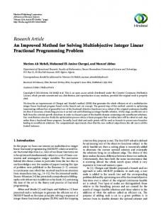
The absolute error between exact solution, y(x), and 8th -order approximation, Y8 (x) which is obtained by the Taylor-successive approximation method is shown in Figure 1. Example 6.4. Consider the nonlinear Abel-Volterra integral equation, Z x 2 y (t) √ y(x) = f (x) + , x−t 0
(6.6)
10
Taylor-successive approximation method for solving nonlinear integral equations
6E-8
5E-8
4E-8
3E-8
2E-8
1E-8
0 0
0.2
0.4
0.6
0.8
1
x
Figure 1: The absolute error, |y(x)−Y8 (x)|, obtained by Taylor-successive approximation method, for example 6.3
with f (x) =
√ 4 √ x − x x, 3
and exact solution y(x) = to this problem yields: Y0 (x) =
(6.7) √ x. Applying the successive approximation method, (3.3,3.4),
√ 4 √ x − x x, 3
√ 4 √ Y1 (x) = x− x x+ 3 √ 4 √ Y2 (x) = x− x x+ 3 .. .
Z
x
0
Z 0
x
√ 4 √ ³ 5´ [ t − t t]2 √ 128 5 512 7 √ √ 3 dt = x − x2 + x2 = x + O x2 45 315 x−t √ 128 5 512 7 2 ³ 7´ [ t− t2 + t2 ] √ √ 8192 7 45 315 √ x2 + · · · = x + O x2 dt = x − 1575 x−t
√ Here, YM (x) converges to exact solution y(x) = x. Since f (x) is not sufficiently smooth, we shall not be able to use the Taylor-successive approximation method to solve this problem. But if we rewrite f (x) in (2.1) as f (x) = f1 (x) + f2 (x)
(6.8)
M.M. Hosseini
11
then by considering (2.4) we have i i−1 +∞ +∞ X X X X N yj − N yj . yi = f1 + f2 + N (y0 ) + i=0
i=1
j=0
j=0
and we can define y0 = f1 , y1 = f2 + N (y0 ), y2 = N (y0 + y1 ) − N (y0 ), .. . So, we can define the following successive approximation method to solve nonlinear functional equation (2.1), Y0 = y0 = f1 , Y1 = y0 + y1 = f1 + f2 + N (y0 ) = f + N (Y0 ), Y2 = y0 + y1 + y2 = f + N (y0 + y1 ) = f + N (Y1 ), and in general YM +1 = y0 + y1 + · · · + yM +1 = f + N (y0 ) + N (y0 + y1 ) − N (y0 ) ± · · · + N (y0 + y1 + · · · yM ) − N (y0 + y1 + · · · yM −1 ) = f + N (y0 + y1 + · · · + yM ) = f + N (YM ), Thus, the M th -order approximation of y(x), YM (x), is easily produced iteratively via the obvious recurrence relation: YM +1 (x) = f + N (YM (x)),
M ≥0
(6.9)
with initial value, Y0 (x) = f1 (x).
(6.10)
Now let us decompose in (6.7) as √ f1 (x) = x, and 4 √ f2 (x) = − x x. 3 In this case, applying the successive approximation method (6.9,6.10), to integral equation (6.6,6.7) implies that √ Y0 (x) = f1 (x) = x, Z x √ 2 Z x 2 √ √ 4 √ [ t] Y0 (t) √ √ dt = x − x x + dt = x, Y1 (x) = f (x) + 3 x−t x−t 0 0 Z x 2 Z x √ 2 √ √ Y (t) 4 √ [ t] √1 √ Y2 (x) = f (x) + dt = x − x x + dt = x, 3 x−t x−t 0 0
12
Taylor-successive approximation method for solving nonlinear integral equations
√ and the exact solution y(x) = x follows immediately. Indeed, we used two iterations only to obtain the exact solution. Numerical results show that, for most example we tested, the Taylor-successive approximation method is more computationally efficient than the successive and the Adomian’s method.
Conclusion A new successive approximation method to solve nonlinear functional equations has been presented. The convergence of this method has been studied and also a computable posteriori error bound has been obtained. In addition, the Taylor-successive approximation method using Taylor series expansion has been suggested that can facilitate calculations. The successive and Taylor-successive approximation methods have been applied to nonlinear Volterra and also nonlinear Fredholm integral equations and the obtained results are compared with the results obtained by the Adomian decomposition method. An important property of the Taylor-successive approximation method is that it accelerates the rapid convergence of the series solution and reduces the size of work without using the so-called Adomian polynomials. The proposed successive approximation methods can be easily generalized to more nonlinear functional equations as well. References [1] G. Adomian. Solving Frontier Problems of Physics: The Decomposition Method. Kluwer Academic Publishers, Dordrecht, 1994. [2] V. Daftardar-Gejji, H. Jafari. An iterative method for solving nonlinear functional equations. J. Mathematical Analysis and Applications, 2006, 316: 753-763. [3] M. Dehghan. The use of adomian decomposition method for solving the one-dimensional parabolic equation with non-local boundary specifications. International Journal of Computer Mathematics, 2004, 81: 25-34. [4] M. Dehghan, F. Shakeri. The use of the decomposition procedure of Adomian for solving a delay differential equation arising in electrodynamics. Physica Scripta, doi: 10.1088/00318949/78/06/065004. [5] M. Dehghan, M. Tatari. The use of the Adomian decomposition method for solving a parabolic equation with temperature overspecification. Mathematical Problems in Engineering, (2006), doi: 10.1155/MPE/2006/65379. [6] I.L. El-Kalla. Convergence of the Adomian method applied to a class of nonlinear integral equations. Applied Mathematics Letters, 2008, 21: 372-376. [7] A. Gorguis. Charpit and Adomian for solving integral equations. Applied Mathematics and Computation, 2007, 193: 446-454. [8] Y.Q. Hasan, L.M. Zhu. A note on the use of modified Adomian decomposition method for solving singular boundary value problems of higher-order ordinary differential equations. Communications in Nonlinear Science and Numerical Simulation, 2009, 14: 3261 - 3265. [9] M.M. Hosseini, H. Nasabzadeh. Modified Adomian decomposition method for specific second order ordinary differential equations. Applied Mathematics and Computation, 2007, 186: 117-123.
M.M. Hosseini
13
[10] M.M. Hosseini, M. Jafari. An efficient method for solving nonlinear singular initial value problems. International Journal of Computer Mathematics, DOI: 10.1080/00207160801965230. [11] A. J. Jerri. Introduction to Integral Equations with Applications, second ed.. WileyInterscience, 1999. [12] Y. Liu. Adomian decomposition method with orthogonal polynomials: Legendre polynomials. Mathematical and Computer Modeling 2009, 49: 1268-1273.