Orifice Pulse Tube cryocooler. Pankaj Kumar. 1. , Ajay Kumar Gupta. 2. , R.K.Sahoo. 3. Mechanical Engineering, Nit, Rourkela, Rourkela, Orissa, INDIA.
IOSR Journal of Mechanical and Civil Engineering (IOSR-JMCE) e-ISSN: 2278-1684, p-ISSN: 2320-334X PP 15-19 www.iosrjournals.org
Approximation Techniques for Solving Cooling Capacity of Orifice Pulse Tube cryocooler Pankaj Kumar1, Ajay Kumar Gupta2, R.K.Sahoo3 Mechanical Engineering, Nit, Rourkela, Rourkela, Orissa, INDIA
ABSTRACT: An approximate numerical analysis is concerned with obtaining approximate solutions for predicting the cooling capacity while maintaining reasonable bounds on errors. Application of the result presented below for a particular numerical model without considering the loss mechanism due to shuttle loss, Regenerator and heat exchanger loss and losses due to conduction. The loss of accuracy with simulation due to a number of gross assumptions in simulation. Although an improved predicted cooling power as well as the pressure/volume relationships for various segments of the refrigerator achieved through a mathematical analysis andin order to improve the accuracy of the model a computer program is developed and runs successfully.
Keywords: Pulse, Tube, Cryocooler, Regenerator, Matlab. I. INTRODUCTION Authors Cryogenics is the science of low temperature (Below 123K). By compressing the gas, the gas is cooled releasing heat and later allowed to expand producing ultra-low temperatures. This is one of the methods to produce low temperature marks the inception of one of the most promising cryogenics refrigerators. Cryocoolers are the devices which produce the required refrigeration power at low temperature. Low cost and high reliability are the crucial factor for the successful applications of cryocoolers. Due to the absence of the moving parts in the cold temperature region and the associated advantages of simplicity and enhanced reliability. The pulse tube system has become one of the most important topics in the field of cryogenics refrigeration. The Pulse Tube refrigerator first conceived in the mid 1960 by Gifford and Longworth appears to be a promising alternative among all the cryocoolers due to the simpler design and the absence of any moving part in the cold head of pulse tube cooler. It has been seemed that in several research papers since from the past 50 years or so on they have suggested towards the development of an appropriate heat transfer correlation between the gas and the pulse tube wall. However explicit correlation that include oscillating and compressing or expanding flows are not available in the literature. This goal can yet to be achieved and verified by the iteration process combining the geometry optimizing process and the numerical simulation. Since there are a several types of pulse tube cryocooler but the question continuation up to the present time and analysing which one will give better performance according to the requirement as per the simplest, low cost or by controlling the volume flow rate according to pressure oscillation discussion in this paper limited to the orifice pulse tube refrigerator.
II. PHYSICAL MODEL AND GOVERNING EQUATIONS 2.1 Physical Model Fig-1 shows a schematic diagram of orifice pulse tube refrigerator. It consist of compressor, aftercooler, regenerator, pulse tube, cold and hot heat exchangers, orifice and reservoir
International Conference on Advances in Engineering & Technology – 2014 (ICAET-2014) 15 | Page
IOSR Journal of Mechanical and Civil Engineering (IOSR-JMCE) e-ISSN: 2278-1684, p-ISSN: 2320-334X PP 15-19 www.iosrjournals.org
Fig.-1Schematic Diagram of OPTR Fig.2.Control Volume patterns at various points In order to simplify the problemssome assumptions need to be made to a point where they can be analysed arelisted below: Pressure and volume oscillations are sinusoidal. Helium, the working gas behaves as a perfect gas. Mass transfer and bulk flow through the orifice, is a function of the pressure amplitude and the average density, ρo : .m = kρo ∆P (k is the mass flow rate tuning constant) Models used thermal equilibrium assumption for the porous zones (regenerator and the heat exchangers) in the OPTR 𝐓𝐡−𝐓𝐜 If a linear profile is assumed then T rg is defined as 𝐓𝐫𝐠 = 𝐓𝐡 𝐥𝐧
𝐓𝐜
In the pulse tube flow is adiabatic and isentropic, such that PV Y = constant. In the cold and hot heat exchangers, the gas temperature is the same as that of the wall temperature of the heat exchanger, which is constant, i.e., heat transfer is perfect in the heat exchanger. The temperature of the reservoir is isothermal. 2.2 Governing Equation A mathematical representation or processes used for analysis of orifice pulse tube refrigerator are presented in this paper .According to the first law of thermodynamics
𝑄 = ∆𝐸 + 𝑊---------- (1) Since, the process is cyclic∆𝐸 = 0. .
.
Therefore,
Q W ------------ (2)
The rate at which work is done is simply
W W X f ---------------- (3)
.
Where f is the frequency of oscillation. If they are sinusoidal, the acoustic power can be written as .
Pv V
1 P1V1 sin ------------- (4) 2 .
Therefore therate of work done due to expansion .
.
.
And Q is equal to Q c i.e. cooling power Q c
.
W can be written as W f
f
1 Pa Va sin --------- (5) 2
1 Pa Va sin ------------ (6) 2
III. DEVELOPMENT OF THE EQUATIONS The phase difference between pressure and mass flow rate is not same at every point due to the compressible flow therefore for the amplitude of volume oscillation are different at the two points. As shown in fig-2 pattern with a series of comprehensive control volume are represented, the patterns are at (1) aftercooler (2) regenerator (3) cold heatexchanger (4) Pulse tube (5) Hot heat exchanger. Applying a discrete volume method to any of the components in the system, the conservation of mass equation for the control volume. For arbitrary control volume in the system, the conservation can be represented as,
International Conference on Advances in Engineering & Technology – 2014 (ICAET-2014) 16 | Page
IOSR Journal of Mechanical and Civil Engineering (IOSR-JMCE) e-ISSN: 2278-1684, p-ISSN: 2320-334X PP 15-19 www.iosrjournals.org . dmn morifics --------------- (7) dt (Negative sign shows that gas flow out of control volume) From Fig. 2, Ma = M5, Mb = M5 + M4, and Mc = M5 + M4 + M 3 + M2 + M1=Moptr The equations below represent the sum of original and varying values for pressure and volume 𝑃𝑖 = 𝑃𝑜 + ∆𝑃𝑖---------- (8) ∆𝑉1 = 𝑉1, 𝑜 − ∆𝑉1------------ (9) ∆𝑉2 = 𝑉2 𝐹𝑖𝑥𝑒𝑑 ---------- (10) ∆𝑉3 = 𝑉3, 𝑜 + ∆𝑉𝑜----------- (11) ∆𝑉4 = 𝑉4, 𝑜 + ∆𝑉3 + ∆𝑉5----------- (12) ∆𝑉5 = 𝑉5, 𝑜 − ∆𝑉5----------- (13) 𝑃𝑉 As we know that PV=MRT or 𝑚 = 𝑅𝑇 Therefore with respect to time for control volume (a) 𝑑𝑀5 𝑑𝑡
1
=
𝑑
𝑅𝑇ℎ 𝑑𝑡
(𝑃5 𝑉5 )----------- (14)
And also 𝑑𝑀5 = − 𝑘𝜌𝑜 ∆𝑃------------- (15) 𝑑𝑡 On equating both equation and substituting the value of 𝑃5 𝑎𝑛𝑑 𝑉5 from equation 5 we get 𝑑𝑀5 1 𝑑 = ((𝑃 + ∆𝑃)(𝑉5,𝑜 − ∆𝑉5 ) 𝑑𝑡 𝑅𝑇ℎ 𝑑𝑡 𝑜 =
𝑑 ∆𝑃 𝑉5,𝑜
−
𝑑𝑡 𝑅𝑇ℎ
𝑑 ∆𝑉5 𝑃𝑜 𝑑𝑡 𝑅𝑇ℎ
i.e. equal to 𝑑∆𝑃 𝑉5,𝑜 𝑑∆𝑉 − 5 𝑑𝑡 𝑅𝑇ℎ
𝑃𝑜
𝑑𝑡 𝑅𝑇ℎ
-------------- (16)
= − 𝑘𝜌𝑜 ∆𝑃 -------------- (17)
Here, let ∆𝑃 = ∆𝑃𝑎 𝑒 𝑖𝜔𝑡 ∆𝑉5 = ∆𝑉5𝑎 𝑒 𝑖𝜔𝑡 . Substituting this into the equation above and taking the time derivative, we are left with an 𝑒 𝑖𝜔𝑡 coefficient in all expressions, which is cancelled to give 𝑉 𝑃 𝑖𝜔∆𝑃𝑎 5,𝑜 − 𝑖𝜔∆𝑉5𝑎 𝑎 = − 𝑘𝜌𝑜 ∆𝑃 ------------(18) 𝑅𝑇ℎ
∆𝑉5𝑎 =
𝑅𝑇ℎ
𝑉5,𝑜 𝑃𝑎
+
𝑘𝜌𝑜 𝑅𝑇ℎ
∆𝑃𝑎 ------------ (19)
𝑖𝜔 𝑃𝑜
Similarly derived for control volume (b) & (c) ∆𝑉3𝑎 = 𝑎 + Where „a‟ is 𝑎 =
𝑉5,𝑜 𝑃𝑎
+
𝑉4,𝑜
+
𝛾𝑃𝑜
𝑉5,𝑜 𝜌𝑜 𝑅𝑇ℎ
𝑘𝜌𝑜 𝑅𝑇ℎ 𝑖𝜔 𝑃𝑜
−
2
𝑉5,𝑜
𝜌𝑜
𝑅𝑇ℎ
𝑘𝜌𝑜
+
+
𝑖𝜔
𝑘 𝑖𝜔
-------------(20)
------------(21)
And ∆𝑉1𝑎 = ∆𝑃𝑎
𝑅𝑇ℎ
𝑉1,𝑜
𝑃𝑜
𝑅𝑇ℎ
Where „b‟ is 𝑉 𝑏 = 𝑎 + 4,𝑜 + 𝛾𝑃𝑜
𝑉5,𝑜 𝜌𝑜 𝑅𝑇ℎ
+
−
𝑉2 𝑅𝑇𝑟
+
𝑉3,𝑜 𝑅𝑇𝑐
2
𝑉5,𝑜
𝜌𝑜
𝑅𝑇ℎ
+
+
𝑏𝑃𝑜 𝑅𝑇𝑐
𝑘𝜌𝑜 𝑖𝜔
− 𝑏𝜌𝑜 + 𝑎𝜌𝑜 +
+
𝑘 𝑖𝜔
𝑉5,𝑜 𝑅𝑇ℎ
+
𝜌𝑜𝑉4,𝑜 𝛾𝑃𝑜
−
𝑎𝑃𝑜 𝑅𝑇𝑐
+
𝑘𝜌𝑜 𝑖𝜔
----------(22)
--------- (23)
Above driving pressure oscillation can be related to an oscillatory volume change at the given control surfaces and can be used for calculating work done and cooling capacity for OPTR as shown in Flow diagram.
International Conference on Advances in Engineering & Technology – 2014 (ICAET-2014) 17 | Page
IOSR Journal of Mechanical and Civil Engineering (IOSR-JMCE) e-ISSN: 2278-1684, p-ISSN: 2320-334X PP 15-19 www.iosrjournals.org
IV. RESULTS AND DISCUSSIONS The graph-1 shows that when orifice is fully closed and open (at very low and high value of „k‟). Fairly large phase difference occurs and low cooling capacity but for middle value of „k‟ the most extreme possible value obtained .Graph-2 shows the effect of frequency on cooling power. As frequency is increasing cooling power is also increasing. Table.1 shoes the calculated data of cooling capacity of 25 Watt and the input date taken from J.H.Baik [4]
Table.1 - Representing Input and Output data Length of the regenerator Diameter of the regenerator Length of the Pulse tube Diameter of the Pulse tube Temperature at cold end Temperature at hot end Cooling Capacity Frequency
0.065 m 0.0602 m 0.0942 m 0.0538 m 70K 300K 25 Watt 2 Hz
100
Phase (deg)
80 60 40 20 0 -16 10
-14
10
-12
10
-10
-8
10
10
-6
10
-4
10
-2
10
k
30
Cooling Power (W)
25 20 15 10 5 0 -16 10
-14
10
-12
10
-10
-8
10
10
-6
10
-4
10
-2
10
k
Graph between cooling power and time interval & between Phase and time interval
V. CONCLUSIONS International Conference on Advances in Engineering & Technology – 2014 (ICAET-2014) 18 | Page
IOSR Journal of Mechanical and Civil Engineering (IOSR-JMCE) e-ISSN: 2278-1684, p-ISSN: 2320-334X PP 15-19 www.iosrjournals.org The behaviour of cooling capacity with orifice opening and with the frequency in an orifice pulse tube refrigerator is analysed using the computer programming method. In an orifice pulse tube refrigerator, here we consider a control volume (a), (b) and (c) as shown in fig-2.and an iterative design process is shown by flow diagram for solving cooling capacity and suggested that considering the loss mechanismwe will get better result,in order to improve the overall cooling capacity of an orifice pulse tube refrigerator
REFERENCE Gifford, W.E. and Longsworth, R.C. Pulse tube refrigeration, Trans ASME B J Eng Industry 86(1964), pp.264-267. Gifford, W.E. and Longsworth, R.C. Pulse tube refrigeration progress, Advances in cryogenic engineering 3B (1964), pp.69-79. David M, Mar_echal JC, Simon Y, Guilpin C. Theory of ideal orifce pulse tube refrigerator. Cryogenics 1993;33:154-61. Alisha R, Design of a Single Orifice Pulse Tube refrigerator Through theDevelopment of a First-Order Model, MassachusettsInstitute of Technology June 2007 R. Radebaugh, "Development of the pulse tube refrigerator as an efficient and reliable cryocooler," 1999-2000. Jong HoonBaik “Design method in active valve pulse tube refrigerator” 2003.
International Conference on Advances in Engineering & Technology – 2014 (ICAET-2014) 19 | Page