TEACHING NEURAL NETWORKS CONCEPTS AND THEIR LEARNING TECHNIQUES Ganesh K. Venayagamoorthy Department of Electrical and Computer Engineering University of Missouri – Rolla, MO 65409, USA
[email protected]
Abstract Neural networks have become increasing popular in the fields of Science and Engineering over the last decade. Most graduate schools in the United States of America and probably in other parts of the world have started offering neural networks as a graduate/postgraduate course. Neural networks are used for nonlinear systems modeling, estimation and prediction of parameters, pattern matching, identification and control. It is necessary that engineering students learn the basics of neural networks somewhere in their undergraduate degree program without taking a full quarter/semester course. This paper presents a software developed in Java to teach basic neural network concepts with backpropagation based learning in a couple of weeks for undergraduate engineering students. This can be done as part of a modeling and simulation course in various disciplines of Engineering. Introduction The role of artificial neural networks in the present world applications is increasing tremendously with applications including speech processing [21, 22], pattern recognition and classification [19, 20], system identification/modeling [23], nonlinear and optimal control [24, 25], time series predictions [18], optimization [17]. Five to ten years ago, a neural network course is thought as a course to be offered at the graduate level for Masters and Doctorate students. But today, this thought could be different since neural network applications are numerous and therefore, is a necessity to introduce neural network basic concepts to students even at the undergraduate level in many engineering disciplines and maybe some science disciplines. The challenge in teaching neural networks to the undergraduate students might be to find a slot in the curriculum to offer a full neural network course. Basic neural networks concepts teaching do not need a full semester or a quarter but probably with the right teaching tools a couple of weeks. Many engineering courses can include a module or two on neural networks depending on the course taught. Teaching technological courses today requires updates every time a course is taught due to the vast amount of research and developments in these disciplines. Additions of
Proceedings of the 2004 American Society for Engineering Education Midwest Section Conference
neural networks modules can be looked at in a similar manner and added to current undergraduate courses. This paper presents a simple software tool developed in JAVA to teach the basic concepts of neural networks and its training with backpropagation. This software is used in introducing neural networks concepts in an experimental course offered at the 300 level to both undergraduate and graduate student at the University of Missouri-Rolla, USA entitled “Computational Intelligence” where neural networks is taught as one of the four paradigms of computational intelligence. The paper is organized as follows: different types of neural networks are discussed first with emphasis on feedforward neural networks, their forward and backward paths for the backpropagation training method. A brief discussion of alternative training algorithms for neural networks is given thereafter. Training procedures (incremental and batch) for neural networks are then described. The Java software developed for teaching neural networks is then presented with some results. Neural Networks Neural networks are known to be universal approximators of any nonlinear function [5] and they are generally used for mapping relationships on nonlinear problems that may have data with noise. There are different types of neural network architectures namely: feedforward, feedback and cellular neural networks. Feedforward neural networks such as the multilayer perceptrons (MLP) are very popular for applications that include large offline data mapping, system identification and others. Feedback neural networks such as recurrent neural networks (RNN) are used to model and control dynamical systems, time series, etc. Cellular neural networks (CNNs) are advanced neural networks where there are interconnections between all neighboring cells. CNNs are used in image processing currently. Training algorithms are critical when neural networks are applied to high speed applications with complex nonlinearities and the training algorithms are different for the different neural network architectures. In this paper, the feedforward neural network is discussed in detail with the backpropagation training [1-5] for implementation in JAVA. A feedforward neural network can consist of many layers as shown in figure 1, namely: an input layer, a number of hidden layers and an output layer. The input layer and the hidden layer are connected by synaptic links called weights and likewise the hidden layer and output layer also have connection weights. When more than one hidden layer exists, weights exist between the hidden layers.
Proceedings of the 2004 American Society for Engineering Education Midwest Section Conference
INPUT LAYER
x
HIDDEN LAYER W1 , 1
Σ
W1 , 2
OUTPUT LAYER V1 , 1
a1
d1 Desired Output
W 2 ,1
Σ
W2 , 2
d2
a2
V2 , 1
y-
+
Σ Error
W 3 ,1
1 (bias)
V 3 ,1
Σ
W3 , 2
W 4 ,1
Σ
W4 , 2
a3
d3
a4
d4
V 4 ,1
TRAINING ALGORITHM
Figure 1 Feedforward neural network with one hidden layer
Neural networks use some sort of "learning" rule by which the connections weights are determined in order to minimize the error between the neural network output and desired output. The following subsections section the two paths involved in a neural network usage – the forward path and the backward path. The backward is described for the backpropagation training algorithm. Other training algorithms are briefly described in a section below. (a). Forward path The feedforward path equations for the network in figure 1 with two input neurons, four hidden neurons and one output neuron are given below. The first input is x and the second is a bias input (1). The activation function of all the hidden neurons is given by (1). ai = Wij X for i =1 to 4, j = 1, 2
(1)
x
where Wij is the weight and X = is an input vector. 1
The hidden layer output called the decision vector d is calculated as follows for sigmoidal functions: di =
1 1 − e(
ai )
for i =1 to 4
(2)
The output of neural network y is determined as follows: d1 d 2 y = [V1 , V 2 , V 3 , V 4 ] d3 d 4
Proceedings of the 2004 American Society for Engineering Education Midwest Section Conference
(3)
(b). Backward path with the conventional backpropagation The serious constraint of the backpropagation algorithm is that the function approximated should be differentiable. If the inputs and desired outputs of a function are known then backpropagation can be used to determine weights of the neural network by minimizing the error over a number of iterations. The weight update equations of all the layers (input, hidden, output) in the multilayer perceptron neural network are almost similar, except that they differ in the way the local error for each neuron is computed. The error for the output layer is the difference between the desired output (target) and actual output of the neural network. Similarly, the errors for the neurons in the hidden layer are the difference between their desired outputs and their actual outputs. In a MLP neural network, the desired outputs of the neurons in the hidden layer cannot be known and hence the error of the output layer is backpropagated and sensitivities of the neurons in the hidden layers are calculated. The learning rate is an important factor in the backpropagation algorithm. If it is too low, the network learns very slowly and if it is too high, then the weights and the objective function will diverge. So an optimum value should be chosen to ensure global convergence which tends to be difficult task to achieve. A variable learning rate will do better if there are many local and global optima for the objective function. Backpropagation equations are explained in more detail in [5, 13] and they are briefly described below. The output error ey is calculated as the difference between the desired output vector yd and actual output y. (4)
e y = yd − y
The decision error vector ed is calculated by backpropagating the output error ey through weight matrix V. edi = ViT e y
for i =1 to 4
(5)
The activation function errors are given by the product of decision error vector edi and the derivatives of the decision vector di with respect to the activations ai. (6)
eai = di (1 − di )edi
The changes in the weights are calculated as ∆V (k ) = γ m ∆V (k − 1) + γ g ey d T ∆W (k ) = γ m ∆W (k − 1) + γ g ea X
T
(7a) (7b)
where γ m is a momentum term, γ g is the learning gain and k is the iteration/epoch number. A momentum term produces a filter effect in order to reduce abrupt gradient changes thus aiding learning. Finally the weight update equations are below.
Proceedings of the 2004 American Society for Engineering Education Midwest Section Conference
W (k + 1) = W (k ) + ∆W (k ) V (k + 1) = V (k ) + ∆V (k )
(8a) (8b)
The learning gain and momentum term have to be carefully selected to maximize accuracy, reduce training time and ensure global minimum . This is where the JAVA software developed for MLP neural networks and presented in this paper is helpful in a classroom environment and elsewhere for students to understand the need to carefully select these parameters and their effects. Other Neural Network Training Algorithms In general, backpropagation is a method used for training neural networks [1-5]. Gradient descent, conjugate gradient descent, resilient, BFGS quasi-Newton, one-step secant, LevenbergMarquardt and Bayesian regularization are all different forms of the backpropagation training algorithm [6, 7]. For all these algorithms storage and computational requirements are different, some of these are good for pattern recognition and others for function approximation but they have drawbacks in one way or other, like neural network size and their associated storage requirements. Certain training algorithms are suitable for some type of applications only, for example an algorithm which performs well for pattern recognition may not for classification problems and vice versa, in addition some cannot cater for high accuracy/performance. It is difficult to find a particular training algorithm that is the best for all applications under all conditions all the time. A number of alternatives and powerful training algorithms to the backpropagation algorithm and its variants exist for more sophisticated neural network architectures in literature [8-12]. A few are briefly described below. (a) Genetic algorithms Genetic Algorithms (GAs) model genetic evolution of nature. They are based on genotypes. The original GA uses string bit representation for the genes. GA is a population based algorithm that uses operators such as selection, crossover, mutation and elitism. It has been reported for training neural networks [16]. The main steps in GA are given below. • Initialize the initial generation of individuals. • While not converged i) Evaluate the fitness of each individual ii) Select parents from the population iii) Recombine selected parents using crossover to get offspring. iv) Mutate offspring v) Select new generation of populations (b) Particle swarm optimization (PSO) Particle swarm optimization is an evolutionary computation technique (a search method based on natural systems) developed by Kennedy and Eberhart [14, 15]. PSO like a generic algorithm (GA) is a population (swarm) based optimization tool. However, unlike GA, PSO has no evolution operators such as crossover and mutation and more over PSO has less number of parameters. PSO is the only evolutionary algorithm that does not implement survival of the
Proceedings of the 2004 American Society for Engineering Education Midwest Section Conference
fittest and unlike other evolutionary algorithms where evolutionary operator is manipulated, the velocity is dynamically adjusted. The system initially has a population of random solutions. Each potential solution, called particle, is given a random velocity and is flown through the problem space. The particles have memory and each particle keeps track of previous best position and corresponding fitness. The previous best value is called as ‘pbest’. Thus, pbest is related only to a particular particle. It also has another value called ‘gbest’, which is the best value of all the particles pbest in the swarm. The basic concept of PSO technique lies in accelerating each particle towards its pbest and the gbest locations at each time step. Acceleration has random weights for both pbest and gbest locations. Figure 2 illustrates briefly the concept of PSO, where Xk is current position, Xk+1 is modified position, Vini is initial velocity, Vmod is modified velocity, Vpbest is velocity considering pbest and Vgbest is velocity considering gbest.
Y
Xk+1 Vmod
t Vgbest
s Vpbest Xk
r Vini X
Figure 2 Position update of a PSO particle (r, s and t are some constants)
i) Initialize a population (array) of particles with random positions and velocities of d dimensions in the problem space. ii) For each particle, evaluate the desired optimization fitness function in d variables. iii) Compare particle’s fitness evaluation with particle’s pbest. If current value is better than pbest, then set pbest value equal to the current value and the pbest location equal to the current location in d-dimensional space. iv) Compare fitness evaluation with the population’s overall previous best. It the current value is better than gbest, then reset gbest to the current particle’s array index and value. v) Change the velocity and position of the particle according to equations (9) and (10) respectively. Vid and Xid represent the velocity and position of ith particle with d dimensions respectively and, rand1 and rand2 are two uniform random functions. Vid = w × Vid + c 1 × rand 1 × ( Pbestid − X id ) + c 2 × rand 2 × ( Gbestid − X id ) X id = X id + Vid
Proceedings of the 2004 American Society for Engineering Education Midwest Section Conference
(9) (10)
vi) Repeat step ii) until a criterion is met, usually a sufficiently good fitness or a maximum number of iterations/epochs. PSO has many parameters and these are described as follows: w called the inertia weight controls the exploration and exploitation of the search space because it dynamically adjusts velocity. Local minima are avoided by small local neighborhood, but faster convergence is obtained by larger global neighborhood and in general, global neighborhood is preferred. Synchronous updates are more costly than the asynchronous updates. Vmax is the maximum allowable velocity for the particles i.e. in case the velocity of the particle exceeds Vmax then it is reduced to Vmax. Thus, resolution and fitness of search depends on Vmax. If Vmax is too high, then particles will move beyond good solution and if Vmax is too low, then particles will be trapped in local minima. c1, c2 termed as cognition and social components respectively are the acceleration constants which changes the velocity of a particle towards pbest and gbest (generally somewhere between pbest and gbest). Velocity determines the tension in the system. A swarm of particles can be used locally or globally in a search space. In the local version of the PSO, the gbest is replaced by the lbest and the entire procedure is same. More details and results are given in [26]. Training Procedures for Neural Networks There are two ways of presenting data to a neural network during training, namely: batch and incremental fashion and these are explained below. (a) Incremental training In this method, each of the input pattern or training data is presented to the neural network and weights are updated for each data presented, thus the number of weight updates will be equal to the size of the training set. The inherent noise of this learning mode makes it possible to escape from undesired local minima of the error potential where the learning rule performs (stochastic) gradient descent. The noise is related to the fluctuations in the learning rule, which is a function of the weights. (b) Batch training In this method, all of the input pattern or training data are presented to the neural network one after the other and then the weights are updated based on a cumulative error function. The process can be repeated over a number of iterations/epochs. In batch mode learning, the network gets struck in a local minimum, in where minimum only depends on the initial network state, the noise is homogeneous, i.e. same at each minimum. JAVA MLP Software A nonlinear function is approximated by a feedforward neural network with an input layer with two inputs (x, a bias of 1), a hidden layer with sigmoidal neurons and a linear output, y. The function approximated by the neural network is y = 2x2+1. The neural network forward and
Proceedings of the 2004 American Society for Engineering Education Midwest Section Conference
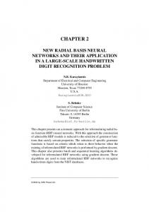
backward operations are coded using JAVA for batch training. The internet explorer or any internet browser can be used to open the JAVA file. The JAVA software screen is as shown in figure 3. The screen allows the user to enter the following values/ranges: input range for x, number of training iterations/epochs, bias value, number of hidden layer neurons, learning gain and momentum term. The screen allows the user to select between training and testing modes. The user can plot the square error curves in both modes by clicking on the respective buttons. The screen outputs the following: minimum and maximum of the actual values of the nonlinear function learned and the corresponding minimum and maximum values estimated by the neural network; the mean square error (MSE) is also displayed for the neural network when in testing mode. Testing mode refers to the neural network subjected to the input when the weights are fixed. Learning is terminated in the testing mode.
Figure 3 The JAVA based neural network software screen
Figure 4 shows a training study for a neural network with 2 hidden neurons (m) learning the function y = 2x2+1 for -2 ≤ x ≤ 2, with 100 epochs (k), with a 0 momentum term γ m, with a 1 learning gain γ g and a bias of 2. It can be seen that there is oscillations around target curve. Figure 5 shows the testing plot of the training study of figure 4. It can be seen that the MSE is over 47586. This shows that neural network did not learn the function at all.
Proceedings of the 2004 American Society for Engineering Education Midwest Section Conference
Figure 4 A training study with k= 100, γg = 1, γm = 0, m = 2
Figure 5 A testing plot of the training with k= 100, γg = 1, γm = 0, m = 2
Proceedings of the 2004 American Society for Engineering Education Midwest Section Conference
Figure 6 shows a training study for a neural network with 2 hidden neurons (m) learning the function for y = 2x2+1 -2 ≤ x ≤ 2, with 2000 epochs, with a 0 momentum term γ m, with a 0.05 learning gain γ g and a bias of 2. It can be seen that there is oscillations around the target curve. Figure 7 shows the testing plot of the training study of figure 4. It can be seen that the MSE is about 2.8088. This shows that neural network is able to approximate the function much better than the case of figure 4. This is due to a lower learning gain and a higher number of training epochs. Large number of training epochs with high learning gain will not produce low MSE during testing. It is necessary to have low learning gains for neural networks to be able to remember what has been presented to it during the training mode. High learning gains force the neural networks to remember very well the last presented input/output data. Generalization is a problem in such cases. Figure 8 shows a testing plot of a training study for a neural network with 5 hidden neurons (m) learning the function y = 2x2+1 for -2 ≤ x ≤ 2, with 100 epochs, with a 0 momentum term γ m, with a 0.2 learning gain γ g and a bias of 2. It can be seen that the neural network approximates the function with some error. The MSE with this case study is about 6.8055. This shows that neural network is able to approximate the function with a lesser number of epochs with 5 hidden neurons with MSE slightly bigger than that of the case in figure 5. This shows that the more the number of hidden neurons the better capability the neural network has to map out a nonlinear function.
Figure 6 A training study with k= 2000, γg = 0.05, γm = 0, m = 2
Proceedings of the 2004 American Society for Engineering Education Midwest Section Conference
Figure 7 A testing plot of the training with k= 2000, γg = 0.05, γm = 0, m = 2
Figure 8 A testing plot of a training study with k= 100, γg = 0.2, γm = 0, m = 5
Proceedings of the 2004 American Society for Engineering Education Midwest Section Conference
Figure 9 shows a testing plot of a training study for a neural network with 5 hidden neurons (m) learning the function y = 2x2+1 for -2 ≤ x ≤ 2, with 100 epochs, with a 0.2 momentum term γ m, with a 0.2 learning gain γ g and a bias of 2. This study shows that the MSE drops to 0.443 with addition of a momentum term of 0.2. The momentum term introduces inertia to the fast updates of weights thus holding the neural network weights from fast abrupt changes. It helps the neural network minimize the MSE further. Figure 10 shows a training study for a neural network with 5 hidden neurons (m) learning the function y = 2x2+1 for -2 ≤ x ≤ 2, with 2000 epochs, with a 0 momentum term γ m, with a 0.03 learning gain γ g and a bias of 2. Figure 11 shows the testing plot of figure 10 with a MSE of about 6.26 × 10⁻⁴ (10-4 is not visible from figure 11; it is at the end of string). This study shows that with a small learning gain, more number of hidden neurons (m=5) and 2000 epochs, MSE comes down a lot. Many other training studies can be carried out to study the effects of the different parameter combinations. The demo software is made available at the author’s website (www.umr.edu/~ganeshv).
Figure 9 A testing plot of a training study with k= 100, γg = 0.2, γm = 0.2, m = 5
Proceedings of the 2004 American Society for Engineering Education Midwest Section Conference
Figure 10 A training study with k= 2000, γg = 0.03, γm = 0, m = 5
Figure 11 A testing plot of a training study with k= 2000, γg = 0.03, γm = 0, m = 5
Proceedings of the 2004 American Society for Engineering Education Midwest Section Conference
Conclusions This paper has presented basic neural network concepts for classroom teaching using a JAVA based software developed at University of Missouri-Rolla, USA. The effects of learning gains, momentum terms, epochs, number of hidden neurons, etc. can be easily conveyed with this type of software tools in a classroom environment when teaching. In addition, this type of software can be made available to students to experiment outside the classroom as homework and come up with a report on effects of different parameters such as the learning gain, number of hidden neurons, momentum term, number of training epochs, etc. for neural network learning. This software demo is currently being upgraded to include other nonlinear functions involving time variables, different training algorithms. With such tools, introducing neural networks into many undergraduate and graduate courses in the engineering and science disciplines does not require much effort and time from the classroom teacher and the students. References [1]. P. J. Werbos, "Backpropagation through time: what it does and how to do it". Proceedings of the IEEE, Vol: 78:10, Page(s): 1550 –1560, Oct. 1990. [2]. P. J. Werbos, The roots of backpropagation, New York: Wiley, 1994. [3]. D. E.Rumelhart, G. E. Hinton, and R. J. Williams, "Learning internal representations by error propagation," in Parallel Distributed Processing, vol.1, cahp.8, eds. D.E.Rumelhart and J.L. McClelland, Cambridge, MA:M.I.T Press, pp.318-62, 1986. [4]. D. E.Rumelhart, G. E. Hinton and R. J. Williams, "Learning representations by back-propagating errors", Nature, Vol.323, pp.533-6, 1986. [5]. S Haykin, Neural networks: A comprehensive foundation, Prentice Hall, 1998, ISBN 0-1327-3350-1. [6]. R. Battit, "First and second order methods of learning: between the steepest descent and Newton's method", Neural Computation, Vol.4:2, pp.141-66, 1991 [7]. M. T. Hagan and M. B. Menhaj, "Training feedforward networks with the Marquardt algorithm" IEEE Transactions on Neural Networks, Vol: 5, 6, pp. 989 –993, Nov. 1994 [8]. J. Salerno, "Using the particle swarm optimization technique to train a recurrent neural model", IEEE International Conference on Tools with Artificial Intelligence, pp.45-49, 1997 [9]. C. Zhang, H. Shao, and Y. Li, "Particle swarm optimization for evolving artificial neural network", Proceedings of the IEEE International Conference on Systems, Man, and Cybernetics, Vol. 4, pp.2487-2490, 2000. [10]. M. Settles and B. Rylander, "Neural network learning using particle swarm optimizers", Advances in Information Science and Soft Computing, pp.224-226, 2002. [11]. F. Van den Bergh and A. P. Engelbrecht, "Cooperative learning in neural networks using particle swarm optimizers," South African Computer Journal, Vol. 26 pp. 84-90, 2000. [12]. S. Lawrence, A. C. Tsoi and A. D. Back, "Function approximation with neural networks and local methods: bias, variance and smoothness", Proceedings of the Australian Conference on Neural Networks, ACNN 96, Canberra, Australia, pp. 16-21, 1996. [13]. B. Burton and R. G. Harley, “Reducing the computational demands of continually online trained artificial neural networks for system identification and control of fast processes”, Proceedings of the. IEEE IAS Annual Meeting, Denver, CO, pp. 1836–1843, Oct. 1994. [14]. J. Kennedy and R. Eberhart, "Particle swarm optimization", Proceedings of IEEE International Conference on Neural Networks, Perth, Australia. Vol. IV, pp. 1942–1948. [15]. J. Kennedy and R. C. Eberhart, Swarm intelligence, Morgan Kaufmann Publishers, 2001. [16]. A. Engelbrecht, Computational Intelligence: An Introduction, John Wiley & Sons, Ltd, England. ISBN 0-47084870-7. [17]. G. K. Venayagamoorthy, “Adaptive critics for dynamic particle swarm optimization”, IEEE International Symposium on Intelligent Control, September 2 – 5, 2004, Taipei, Taiwan, pp. 380 -384. [18]. X. Cai X, N. Zhang, G. K. Venayagamoorthy, D. C. Wunsch, “Time series prediction with recurrent neural networks using a hybrid PSO-EA algorithm”, IEEE-INNS International Joint Conference on Neural Networks, Budapest, Hungary, July 24 -29, 2004.
Proceedings of the 2004 American Society for Engineering Education Midwest Section Conference
[19]. V. Venayagamoorthy, D. Allopi, G. K. Venayagamoorthy, "Neural network based classification of road pavement structures", International Conference on Intelligent Sensing and Information Processing, Chennai, India, January 4 - 7, 2004, pp. 295 – 298. [20]. S. Chetty, G. K. Venayagamoorthy, “A neural network based detection of brain tumours using electroencephalograph”, International Conference on Artificial Intelligence and Soft Computing, Banff, Canada, July 2002, pp. 391 – 396. [21]. V. Moonasar, G. K. Venayagamoorthy, “A committee of neural networks for automatic speaker recognition”, IEEE-INS International Joint Conference on Neural Networks 2001, Washington DC, USA, vol.4, pp. 2936 2940. [22]. G. K. Venayagamoorthy, N. Sunderpersadh, “Comparison of text-dependent speaker identification methods for short distance telephone lines using artificial neural networks”, IEEE-INNS International Joint Neural Networks Conference (IJCNN 2000), 24 – 27 July, 2000, Como, Italy, pp. 253 - 258. [23]. G. K. Venayagamoorthy, R.G. Harley, "A continually online trained artificial neural network identifier for a turbogenerator", IEEE International Electric Machines and Drives Conference IEMDC 99, Seattle, USA, 9 - 12 May 1999, pp. 404 - 406. [24]. G. K. Venayagamoorthy, R. G. Harley, “A continually online trained neurocontroller for excitation and turbine control of a turbogenerator”, IEEE Transactions on Energy Conversion, vol. 16, no.3, September 2001, Page(s): 261-269. [25]. J. W. Park, R. G. Harley, G. K. Venayagamoorthy, “Adaptive critic based optimal neurocontrol for synchronous generator in power system using MLP/RBF neural networks”, IEEE-IAS Industry Applications Transactions, vol. 39, no. 5, September/October 2003, pp. 1529 - 1540. [26]. V. G. Gudise, G. K. Venayagamoorthy, “Comparison of particle swarm optimization and backpropagation as training algorithms for neural networks”, IEEE Swarm Intelligence Symposium, Indianapolis, IN, USA, April 24 -26, 2003, pp.110 - 117.
Acknowledgment The support from the National Science Foundation under CAREER Grant: ECS # 0348221 and the University of Missouri Research Board is gratefully acknowledged for this work.
Biography Ganesh Kumar Venayagamoorthy received the B.Eng. (Honors) degree with a first class in electrical and electronics engineering from the Abubakar Tafawa Balewa University, Bauchi, Nigeria, and the M.Sc.Eng. and Ph.D. degrees in electrical engineering from the University of Natal, Durban, South Africa, in March 1994, April 1999 and February 2002, respectively. He was appointed as a Lecturer with the Durban Institute of Technology, South Africa during the period March 1996 to April 2001 and thereafter as a Senior Lecturer from May 2001 to April 2002. He was a Research Associate at the Texas Tech University, USA in 1999 and at the University of Missouri-Rolla, USA in 2000/2001. He joined the University of Missouri-Rolla, USA as an Assistant Professor in May 2002. His research interests are in computational intelligence, power systems, control systems and digital systems. He has authored about 100 papers in refereed journals and international conferences. Dr. Venayagamoorthy is a 2004 National Science Foundation, USA CAREER award recipient, the 2003 International Neural Network Society Young Investigator award recipient, a 2001 recipient of the IEEE Neural Network Society summer research scholarship and the recipient of five prize papers with the IEEE Industry Application Society and IEEE Neural Network Society. He is a Senior Member of the Institute of Electrical and Electronics Engineer (IEEE), USA, and South African Institute of Electrical Engineers (SAIEE). He was Technical Program Co-Chair of the International Joint Conference on Neural Networks (IJCNN), Portland, OR, USA, July 20 – 24, 2003 and the International Conference on Intelligent Sensing and Information Processing (ICISIP), Chennai, India, January 4 – 7, 2004. He is founder and currently the Chair of IEEE St. Louis Computational Intelligence Society Chapter.
Proceedings of the 2004 American Society for Engineering Education Midwest Section Conference