Augmented Neural Networks and Problem-Structure Based Heuristics for the Bin-Packing Problem
Nihat Kasap Faculty of Management, Sabanci University Orhanli – Tuzla, 34956, Istanbul, Turkey
[email protected] and
Anurag Agarwal* Department of Information Systems and Operations Management Warrington College of Business Administration University of Florida, Gainesville, FL 32611-7169 USA
[email protected]
*Corresponding author
Augmented Neural Networks and Problem-Structure Based Heuristics for the Bin-Packing Problem Abstract In this paper, we apply the Augmented-neural- networks (AugNN) approach for solving the classical bin-packing problem (BPP). AugNN is a metaheuristic that combines a priority- rule heuristic with the iterative search approach of neural networks to generate good solutions fast. This is the first time this approach has been applied to the BPP.
We also propose a
decomposition approach for solving harder BPP, in which sub problems are solved using a combination of AugNN approach and heuristics that exploit the problem structure. We discuss the characteristics of problems on which such problem-structure based heuristics could be applied. We empirically show the effectiveness of the AugNN and the decomposition approach on many benchmark problems in the literature. For the 1210 benchmark problems tested, 917 problems were solved to optimality and the average gap between the obtained solution and the upper bound for all the problems was reduced to under 0.66% and computation time averaged below 33 seconds per problem. We also discuss the computational complexity of our approach.
Key Words: Bin Packing, Heuristics, Neural Networks, Optimization
2
1. Introduction The one-dimensional bin-packing problem (BPP) invo lves minimizing the number of fixedcapacity bins required to pack n items of various sizes (or weights). This problem occurs frequently in distribution, production and task/resource allocation and cutting stock problems. For example, in distribution, packing containers for trucks/trains involves the BPP.
In
production, scheduling tasks on machines in shifts can be considered a BPP if we treat shifts as bins, and tasks as items. Like most optimization problems, the BPP belongs to the class of NPhard problems (Garey and Johnson, 1979, Martello and Toth, 1990). Many heuristics and metaheuristics exist in the literature for generating good approximate solutions fast for the BPP. Heuristics are based on some kind of priority or dispatching rule such as ‘first- fit descending’ (FFD) or ‘best- fit descending’ (BFD). These heuristics produce good approximate solutions very fast and therefore can be applied to large problems, but they fail to make use of problemspecific structures and leave significant gaps from the optimal. Metaheuristics include iterative approaches such as tabu search, simulated annealing and genetic algorithms. These techniques find improved solutions, because they search a larger solution space. Depending on the number of iterations required, these metaheuristics may take very long and therefore not be suitable for solving very large problems in reasonable time. In this paper we apply a neural-network based approach called Augmented Neural Networks (AugNN) for the BPP, and also a decomposition approach involving heuristics that exploit the problem structure. AugNN is a metaheuristic that takes advantage of both the heuristic and the iterative search approach.
In this approach, the bin-packing problem is
formulated as a neural network of input, hidden and output layer of nodes, with weights associated with links between nodes, much like in a neural network. 3
Input, output and
activation functions are designed to (i) capture and enforce the constraints of the problem, and (ii) apply a particular heuristic, such as FFD or BFD, to assign an item to a bin in each iteration. After n iterations, or an epoch, n assignments take place and a feasible solution is generated. Weights are modified after each epoch, allowing a neighboring feasible solution to be generated in subsequent epochs. If improvements are found, the weights are reinforced, otherwise not. After some epochs, the network learns a good set of weights that generate good solutions. Thus, a non-deterministic local search is performed by perturbing the data using weights.
This
approach was first introduced by Agarwal et al. (2003) for the task-scheduling problem. We apply the AugNN approach in conjunction with two well-known heuristics, namely FFD and BFD, on many benchmark problem sets in the literature. These problem sets fall under three levels of difficulty – easy, medium and hard. For the easy and medium problems, the AugNN approach found the best-known upper-bound solutions in 909 out of 1200 problems and improved upon the heuristic solution on the remaining problems and gave an overall gap of 0.375% from known optimum solutions. For the hard benchmark problems, the AugNN approach failed to provide very good results in reasonable time. For these hard problems, we propose a decomposition approach in which we decompose the problem into sub problems and solve the sub problems using heuristics that exploit the structure of the problem. Using this decomposition strategy, upper-bound solutions were found for 8 out of 10 hard problems and within 1 bin of the upper bound for the remaining 2 problems. All 10 solutions were found in less than 0.25 seconds each. We thus make a two-fold contribution to the bin-packing literature. First, we propose an AugNN formulation for the first time for the BPP and show its effectiveness in terms of improving upon a heuristic solution.
Second, we propose new heuristics that exploit the
problem structure and solve the BPP using a decomposition strategy. Although the problem4
structure based heuristic, as the name suggests, may not be generalized, the lessons learnt from solving the hard benchmark problems may be applied to other bin-packing problems. We discuss the conditions under which some types of problem-structure based heuristics can be applied. The rest of the paper is organized as follows. In Section 2, we review the relevant binpacking literature. We explore the various heuristics used for this problem. In the following section, we provide the details of the AugNN formulation for the BPP. We explain the neuralnetwork architecture for the BPP and present all the functions needed to solve the problem. Search strategies are also discussed. Section 4 describes our decomposition approach, including the problem-structure based heuristics for solving the hard benchmark problems. In Section 5, we present our computational results.
Section 6 provides the summary, conclusions and
suggestions for future research.
2. Literature Review Since the BPP is NP-hard in the strong sense (Garey and Johnson, 1979), a polynomial time algorithm to solve it optimally does not exist and is unlikely to be discovered in the future. Scholl et al. (1997) provide a good survey of extant solution procedures, and also propose a new heuristic that is a combination of tabu search and a branch-and-bound procedure based on known and new bound arguments and a new branching scheme. They study the well-known heuristics such as FFD, BFD, and worst fit descending (WFD) as well as the B2F heuristic, which works like FFD until a bin is filled then tries to exchange the smallest item assigned to the bin with two small-sized items not currently assigned such that the residual capacity is decreased. Valerio de Carvalho (1999) gives an exact algorithm based on column generatio n and branch-and-bound. Gupta and Ho (1999) give a heuristic called ‘minimum bin slack’ to
5
solve the BPP. This heuristic is bin centric. At each step, an attempt is made to find a set of items (packing) that fits the bin capacity as much as possible. The worst-case performance of heuristics for BPP has been studied in Anily et al. (1984). Many metaheuristics have been proposed in the bin-packing literature, such as, genetic algorithms (GAs), tabu search, simulated annealing (SA) and ant colonies (AC). However, no study has focused on a neural- network approach in the bin-packing literature. In most cases GAs were found to be relatively inefficient. As explained in (Reeves, 1995), the complexity of the traditional GAs was high because of the length of the chromosome string required. Many of the solutions generated in each generation were infeasible and checking the feasibility of each generated solution was very time consuming. Reeves (1995) proposed hybrid GAs aimed at improving the performance of traditional GAs.
The performance improved for small size
problems, both in terms of probability of finding the optima and the processing time. However, the solution quality for the larger size problems was not improved. Another GA approach was used in (Corcoran and Wainwright, 1993). Performance is improved by using two mechanisms - sliding window mechanism to identify highly fit sequences and reduction mechanism to preserve fit sequences. Therefore, highly fit members can quickly dominate the populatio n and cause the GA to converge more quickly. Several new heuristics for solving the one-dimensional BPP are presented in (Fleszar and Hindi, 2002). Some improvements on minimal-bin-slack heuristic have been made. They show that their heuristics are very efficient even though they have high computational complexity. Variable neighborhood search has also been developed and used in (Fleszar and Hindi, 2002). SA approach has also been used in (Brusco et al, 1997, Rao and Iyengar, 1994). The performance of SA with morphing is sensitive to parameter choices. They have shown that no single version of their heuristic particularly dominates other procedures in terms of solution 6
quality. However, there is a notable difference in performance associated with the different cooling factors. Gradisar et al. (1999) proposed a hybrid approach of combining pattern-oriented LPbased method and the item-oriented sequential heuristic procedure.
Their objective of
optimization is cutting order lengths into exact required number of pieces and cumulating residual lengths into one piece suitable for later use. They mentioned that the method is especially useful when average number of pieces cut out of an average stock length is large and when the cost of changing the cutting pattern is low. Alvim et al. (2004) propose a hybrid improvement procedure for the bin packing problem. Their heuristics has several features such as the use of lower bounding strategies, the generation of initial solution by reference to the dual min-max problems, the use of load redistribution based on dominance and improvement process utilizing tabu search. Their procedure compares favorable with all other heuristics in the literature. Their algorithm is the only one that has succeeded in finding the best known results for all instances by using a single heuristics. Considering that the best results previously reported in the literature were not all of them obtained by a single heuristics our proposed solution method is still encouraging. Loh et al. (forthcoming) develop a new procedure that uses the concept of weight annealing to solve the one-dimensional bin packing problem. Their procedure is straightforward and easy to follow. They find that their procedure produce very high-quality solutions very quickly and generates several new optimal solutions.
7
3. The AugNN Framework We first describe the problem formally and then present the AugNN framework.
3.1 Problem Description The BPP consists of packing a set of items into minimum number of bins such tha t the total size (or weight) does not exceed a maximum value (bin capacity). In other words, we define a binpacking problem (BPP) as follows: •
We are given a finite set of n items each having a certain size.
•
We define a group to be a subset of items such that the total size of the group does not exceed the bin capacity.
•
The primary goal is to create a feasible solution with the minimum number of groups.
3.2 Neural Network Architecture In the AugNN approach, we formulate the BPP as a neural network. Figure 1 shows the neuralnetwork architecture and the correspondence with the BPP graphically. Each item and each bin is represented as a processing element (PE) of a neural network. The item PE nodes, denoted by T1 , T2 ,…,Tn , constitute the item layer, similar to the input layer of a neural network. Similarly, the bin PE nodes, denoted by B1 ,B2 ,…,Bm, constitute the bin layer, which corresponds to the hidden layer of a neural network. There is also an output layer with one node, called the ‘Final node’, designed to capture the outputs of the bin and item layers. For ease of formulation, we also add a dummy initial node linked to the item- layer nodes. It keeps track of the numbers of epochs and iterations. Nodes in the item layer get an input signal from the initial node through links.
The item nodes are fully connected to the nodes of the bin layer through links
characterized by weights, denoted by ? 1 , ? 2 ,…,? n . The item nodes are also connected to the final node. Each bin node, except the rightmost, is connected to the bin node to its right. Bin nodes are also connected to item nodes, to signal assignment.
take in Figure 1
8
For each set of nodes, including the initial, the item, the bin and the final node, we define input, output and activation functions, just like in neural networks.
These functions are
designed to (i) capture the constraints of the bin-packing problem and (ii) assign an item to a bin in one iteration, using a certain priority rule heuristic, such as FFD or BFD. After n iterations, the network produces a solution, i.e., the number of bins used. We call a set of n iterations an epoch, much like in neural-network training. At the end of an epoch, the weights are modified using a search strategy and a new epoch starts. Learning takes place in each epoch. The search strategy involves reinforcing the weights if an improved solution is found, and backtracking to the last best set of weights if no improvement occurs over a pre-specified number of epochs. On an average, in less than 145 epochs, the AugNN approach found very good solutions for the 1210 test problems. The activation functions are used to capture the state of a PE. For example, for the item nodes, the state would indicate whether that item has been assigned or not. For the bin node, it would indicate whether the bin is open, packed, or not yet opened. We now describe the mathematical formulation and algorithmic details of AugNN for the BPP.
3.3 Notation n m T B C k t I F Ti Bj Si SUI
: Number of items : UB(Number of bins) : Set of items = {1,2,…,n} : Set of bins = {1,2,…m } : Capacity of bins : Epoch number. : Current assignment iteration [0,n] : Initial node : Final node : ith item node in the item layer, i ∈ T : jth bin node in the bin layer, j ∈ B : Size of item i, i∈ T : Set of unassigned items. 9
LB UB RF BF α
: Lower bound of the number of bins : Upper bound of the number of bins : Reinforcement factor : Backtracking factor : Search coefficient
Following are all functions of assignment iteration t : IFI(t) : Input function of the initial node IFTi(t) : Input function of item nodes Ti, , i ∈ T IFBij(t) : Input function of bin nodes Bj from Item nodes Ti, i ∈ T, j ∈ B IFFT(t) : Input function of the final node from the item nodes IFFB(t) : Input function of the final node from the bin nodes OFI(t) OFTBi(t) OFTFi(t) OFBF j(t) OFBT ji(t) OFBBj(t) OFFI(t)
: Output function of initial node : Output function of item nodes Ti to bin nodes, i ∈ T : Output function of item nodes Ti to final node, i ∈ T : Output function of bin nodes Bj to final node, j ∈ B : Output function of bin nodes Bj to item node Ti, i ∈ T, j∈ B : Output function of bin nodes Bj to Bj+1 , j ∈ B, j ≠ m : Output function of final node
θI(t) θTi(t) θBj(t) θF(t) assignij(t) RCj(t)
: Activation function of the initial node : Activation function of item nodes Ti, i ∈ T : Activation function of bin nodes Bj, j ∈ B : Activation function of the final node : Item i assigned to bin j, i ∈ T, j ∈ B : Residual capacity for j th bin, j ∈ B
Following are functions of k: OFF(k) : Output function of final node. ωi(k) : Weight on links from item nodes Ti to bin nodes, i ∈ T ε(k) : Error or difference between solution and lower bound in epoch k
3.4 Preliminary Steps 1. Calculate the lower bound i.e. the minimum possible number of bins needed Lower Bound = ( ∑ Si ) / C ) i∈T
2. Calculate the upper bound i.e. the maximum possible number of bins needed Upper Bound = n /(C / Max( S i )) , i ∈ T i
We want to use this many bins in the hidden layer. m = UB(number of bins). 3. Weights ωi (0) are initialized at 1.00.
3.5 AugNN Functions
10
We present here the input, activation and output functions of each layer of nodes, starting with the initial node, followed by item nodes, bin nodes and then the final node.
3.5.1 Initial Node t = 0 to begin with.
Input function IFI(0) = 1 IFI(t) = OFFI(t), for t > 0 The initial node gets an initial signal of 1 at the beginning to set off the first iteration of the first epoch. Thereafter, it receives an input from the final node.
Activation State The state of the initial node is defined by t and k, where t is the assignment number and k is the epoch number. ?I(0): { t = 1, k = 1 For t > 0,
t = t + 1, k = k if IFI (t ) = 1 θ I (t ) = t = 1, k = k + 1 if IFI (t ) = 2 t = 0, k = 0 if IFI (t ) = 3 At the beginning, when t = 0, both t and the k are initialized at 1. IFI of 1 indicates a new assignment iteration for the same epoch. So, t is incremented by one, while k remains the same. At the end of an epoch, signified by IFI of 2, k is incremented by 1 while t is initialized to 1. At the end of the problem, i.e. when IFI is 3, both t and k are 0.
Output function 1, if t > 0 OFI (t ) = 0, otherwise Whenever t > 0, the problem needs to be solved, so the initial node sends an output signal of 1 to the item nodes, signaling that if they are not yet assigned, it is time to get assigned.
3.5.2 Item Layer Input function IFTi(t) = OFI(t) , i ∈ T
11
Activation function ∀ i ∈ T, j ∈ B, θTi(0)=1 0, if θ Ti (t − 1) = 0 ∨ (θ Ti ( t − 1) = 1 ∧ OFBT ji (t ) = 1), t > 0 θ Ti (t ) = 1, if θ Ti (t − 1) = 1 ∨ (θ T i( t − 1) = 0 ∧ IFI i (t ) = 2)
State 1 above implies that item node Ti has not been assigned yet. State 0 implies that it has been assigned. Initially (i.e. at t=0) the state of all item nodes is initialized to 1. When the item is assigned (signified by OFBT ji (t) = 1), its state changes to 0 and stays that way for the rest of the current epoch. The state changes back to 1 when a new epoch starts (i.e. when IFI is 2). Output function ∀i∈T OFTBi (t) =
θTi(t)* Si * ωi(k)
1, if θ Ti (t ) = 0 OFTFi (t ) = 0, otherwise The OFTB signal sends a weighted size to the bin layer. OFTB is 0 if the item is already
assigned (due to θTi (t) = 0), and positive if not yet assigned. OFTF sends a signal to the final node indicating that the item has been assigned (indicated by θTi (t)=0)..
3.5.3 Bin layer For the bin layer, we explain the activation function first, since it is used in the input function.
Activation function RC j(1) = C θB1 (1)= 1 state of the first bin for the first assignment iteration is 1 (open). j > 1∧ j ∈B θBj(1)= 0 0, if θ B j (t − 1) = 0 ∨ IFI (t ) = 2 θ B j (t ) = 1, if θ B j (t − 1) = 1 ∨ (θ B j (t ) = 0 ∧ OFBB j −1 (t ) = 1) 2, if θ B j (t − 1) = 1 ∧ ( RC j (t ) < Min[ Sl ], l ∈ SUI
12
: bin not open yet : bin open : bin packed/closed
RC j(t) = RCj(t) – Si
where i is the index for Max OFTBi(t)
At the beginning the first bin is open, rest are unopened. A new bin opens (i.e., assumes state 1) when it receives a signal (OFBBj-1 (t))from the previous bin. The previous bin sends this signal when it cannot fit the item with maximum OFTBi(t). When an open bin’s residual capacity is less than the minimum size unassigned item, then the bin closes (state 2).
Input function ∀ i ∈ T, j ∈ B Max (OFTB j (t )) , if IFB j (t ) = i 0 if
θ B j (t ) = 1 θ B j (t ) = 0 ∨ θ B j (t ) = 2
If the bin is open (state of 1) then it accepts the maximum output of the item nodes as its input. If the bin is not yet open (state 0) or packed and closed (state 2), it does not accept any input.
Assignment of item to bin 0, if Si > RC j (t ) assignij (t ) = 1, if Si ≤ RC j (t ) where i is the index for Max OFTBi (t)
Since we are applying FFD and BFD, once an item is assigned to a bin, the rest of the bins do not attempt to pack the same item.
Output function ∀ i ∈ T, j ∈ B
1, if θ B j (t ) = 2 OFBF j (t ) = 0, otherwise
When a full bin closes (state 2), it sends a signal to the final node. The final node keeps a counter of the number of bins in state 2. 1, if θ B j (t − 1) = 1 ∧ RC j (t ) < Si ( t ), i is the index for MaxOFTBi (t ) OFBB j (t ) = 0, otherwise
13
When a bin cannot accept the biggest item due to small residual capacity, it sends a signal to the next bin to open.
1, if assignij (t ) = 1 OFBTji (t ) = 0, otherwise When a bin accepts an item, it sends a signal of 1 to the item node.
3.5.4 Final Node Input function The final node receives two sets of inputs. One from the bin layer (IFFB) and one directly from the item layer (IFFT). m
IFFB (t ) = ∑ OFBF j (t ) j =1
n
IFFT( t ) = ∑ OFTFi (t ) i =1
IFFB is essentially the sum of all filled bins. IFFT is the sum of all assigned items.
Activation function 0, if θ F (t ) = 1, if 2, if
IFFT (t ) < n IFFT (t ) = n IFFT ( t ) = n ∧ IFFB (t ) = LB
State of 0 implies that not all n items are assigned. State of 1 implies that all items are assigned, which is an indication of the end of the current epoch. State of 2 implies that a lower bound solution has been found and therefore the processing can stop.
Output function 1, if θ F (t ) = 0 OFFI (t ) = 2, if θ F (t ) = 1 ∧ k < kmax 3, if θ F (t ) = 1 ∧ k = k ( max ) ∨ θ F (t ) = 2
OFF(k) = IFFB(t), if OFFI(t) = 2 or 3. Output OFFI of 1 implies that not all items have been assigned and the network should run a new assignment iteration. Output OFFI of 2 implies that all items have been assigned but 14
the lower-bound solution has not reached and the number of epochs has not reached the max, so the network should run another epoch. Output OFFI of 3 acts as a stopping rule. If either a lower-bound solution is found or the number of epochs has reached its preset max limit, the network stops. The output OFF represents the solution, i.e. the number of bins used to fill all the items.
3.5.5 Order of Evaluation of Functions It is important to understand the order in which these functions are evaluated. The ordering is as shown in Figure 2. In general, in neural networks, input function is calculated first, followed by activation function followed by the output function. Further, in feed forward neural networks, input layer functions are followed by hidden layer functions, followed by output layer functions. In AugNN, we deviate slightly because of (i) the assignment function and (ii) need to open new bins if existing bins cannot fit an item. This requires evaluating certain functions within the same layer twice. One of the advantages of this kind of formulation is that coding becomes easier. Also, a different heuristic, such as ‘worst fit descending’ can be applied by slightly modifying one of the functions above. take in Figure 2
3.6 Search Strategy A search strategy is required to modify the weights. Weights are modified once for each epoch. They are not modified from one assignment iteration to the next. The idea behind weight modification is that if the error in an epoch is too high, then the order in which items should be placed should be changed more than if the error is less. We employ the following search strategy. ωi(k+1)= ωI(k) + α * Si * ε(k) ∀ i ∈ T where ε(k) = OFF(k) - LB In addition, we employ reinforcement and backtracking mechanisms to improve the solution quality.
3.6.1 Reinforcement 15
Whenever the solution improves in the current epoch compared to the previous epoch, i.e. whenever OFF(k) < OFF(k -1), we reinforce the weights by magnifying the increases made during the previous epoch. We employ a reinforcement factor RF as follows: ωI(k) = ωI(k) + RF * (ωI(k) - ωI(k-1) ), ∀ i ∈ T Such reinforcement acts as a reward for finding a better solution and helps preserve the relative weights of the items for a few epochs. RF can be any real number between 1 and infinity, although we found through some experimentation, that RF value of 3 gave good results.
3.6.2 Backtracking If the solution does not improve for a certain number of epochs say 100 or 150, then it is advisable to backtrack to the previous best solution and forget the last few epochs and start over. This backtracking mechanism prevents the network from following a path of no improvement for any longer than necessary.
We use a parameter called backtracking factor (BF) to
implement such backtracking.
3.7 End of iteration routines 1.
If OFFI is 1, do not modify the weights and start with the next assignment iteration.
2.
If OFFI is 2, it signifies the end of an epoch. Do the following steps: a. check if the current solution is the best so far. If so, store it as best solution. Also, store the current weights as best weights. b. Calculate the error i.e., the difference between OFF(k) and the lower bound. c. Sense if reinforcement needed.
If needed, apply reinforcement using the
reinforcement strategy. d. Sense if backtracking needed. If needed, apply backtracking. e. Modify weights, using the search strategy. 3.
If OFFI is 3, stop the network, and display the best result so far.
3.8 Computation Complexity The computational complexity of the FFD and BFD is O(n log n), primarily because sorting is required. Once the sorted list of unassigned items is available, the assignment is linear in n, or O(n). The complexity of AugNN is the same for each epoch, i.e. O(n log n). Of course, time taken is more because of the number of epochs needed.
16
4. Decomposition Strategy and Problem-Structure Based Heuristic For the set of hard instances, although AugNN improved significantly over the single-pass FFD and BFD, thus reducing the gap significantly from the upper bound, the gap was still too high. To reduce the gap further, we propose a decomposition strategy - breaking the problem into sub problems and solving them using heuristics that exploit the problem structure. Most heuristics are item centric, i.e. you take an item, in a certain order of size, and decide which bin it goes in. Our proposed heuristics are bin centric, similar to Gupta and Ho’s (1999) ‘minimum bin slack’ heuristic, in which we take a bin and pack it with appropriate items with minimum residual capacity in each bin. Ours is a special case of the ‘minimum bin slack’ heuristic designed for a fixed number of items and involves a factor called tolerance for residual capacity. We observed that for each of the ten hard problems, the maximum number of items that could fit in a bin was four, because even the five smallest items would exceed the bin capacity. So the trick was to first fill as many bins as possible with four items each, with minimum residual capacity, within a given tolerance. This became our first sub problem – i.e., fitting bins with four items within a tolerance. The next sub problem involved fitting as many bins as possible with three items within tolerance. All remaining items were treated as the third sub problem, and solved using AugNN. In designing our ‘pack-four item bins’ and ‘pack-three item bins’ heuristics, we exploited the fact that the item sizes were drawn from a uniform distribution. With the help of Figures 3a and 3b, we will explain how. In Figures 3a and 3b, we plot the items on the x-axis in the increasing order by size and we plot sizes on the y-axis. Since the sizes are drawn from a uniform distribution, we get a near-straight line plot. For the case of four - item packing let us look at Figure 3a. Suppose we find four adjacent items ‘c’, ‘d’, ‘e’ and ‘f’, such that the sum of their sizes is closest to but within the bin capacity. This group of four items can be placed in a bin. Due to the linearity of 17
the plot, if we find a pair of adjacent items on either side of and equidistant from items ‘c’, ‘d’, ‘e’ and ‘f’, then the sum of the sizes of these four items should be close to the bin capacity. For example, items ‘a’ and ‘b’ on the left and items ‘g’ and ‘h’ on the right, equidistant from ‘c’, ‘d’, ‘e’ and ‘f’, should fit in a bin tightly. Extending this idea further, the sum of the sizes of items ‘j’ and ‘k’ and ‘p’ and ‘q’ will also be close to the bin capacity, assuming that ‘j’ and ‘k’ are about as far from ‘a’ and ‘b’ as ‘p’ and ‘q’ are from ‘g’ and ‘h’. Using this idea, we can find groups of four items that can be packed in a bin with little residual capacity, within a certain tolerance. Notice that the complexity of this heuristic is linear in n. _________________________ take in Figure 3 __________________________
For the three- item bin packing heuristic, we make a similar observation. In Figure 3b, for example, sum of the sizes of items ‘a’, ‘c’ and ‘d’ will be about the same as that of items ‘b’, ‘c’ and ‘e’, assuming items ‘a’ and ‘b’ are as far from item ‘c’ as items ‘d’ and ‘e’. Of course, we are assuming that the size ranges, with respect to bin capacity, are such that three items can fit tightly. Note that if the sizes of items were drawn from a distribution other than uniform, such as, normal or exponential, we would not get a near-straight line plot in Figures 3a and 3b, and we couldn’t find groups of four (or three) items to pack in this manner. For the non-uniform distribution case, the proposed heuristics would not work. Based on the above observations, we outline the ‘Pack Four-Item’ heuristic and the ‘Pack Three-Item’ heuristic below, for solving the first and the second sub problems. Sub Problem 1: Pack Four-Item Bins
18
Step 1: Sort the items from smallest to largest. Step 2: Open a new bin. Step 3: Place the two smallest items in the open bin. Step 4: Calculate the residual capacity of this bin and divide by two. Step 5: Find the item with size closest to but less than the value obtained in Step 4, within a pre specified tolerance (in this case 500, but could be different for a different problem). If item found then place it in the bin and go to Step 6, else go to Step 10. Step 6: Find the new residual capacity. Step 7: Find the item with size closest to but less than the value obtained in Step 6 within a pre specified tolerance (in this case 500, but could be different for a different problem). Note that this fourth item should be found either adjacent to or very close to the third item. If found then place it in the bin and go to Step 8, else go to Step 10. Step 8: Close the bin and count it as a packed bin. Step 9: Remove these four items from the list of unassigned items and go to Step 2. Step 10: Do not commit any items to this bin, close the bin and do not count it as a packed bin. Give the total number of packed bins so far. Go to Sub Problem 2. Sub Problem 2: Pack Three-item Bins. Step 1: Sort the list of unassigned items from largest to smallest. Step 2: Open a new bin. Step 3: If there are at least three items in the set of unassigned items then, place the largest and the smallest items in this bin. Step 4: Find the residual capacity of this bin. Step 5: Find the item closest to but less than the value obtained in Step 4, within a pre specified tolerance (in this case 1000, but could differ). If such an item found then place it in the bin and go to Step 6. If not, go to Step 8. Step 6: Close this bin and count it as a packed bin. Step 7: Remove these three items from the list of unassigned items and go to Step 2. Step 8: Do not commit any items to this bin, close the bin and do not count it as a packed bin. Give the total number of packed bins so far. Go to Sub Problem 3. Sub Problem 3: AugNN
19
Step 1: Enlist all the remaining unassigned items. Step 2: Apply AugNN for this set of items. Finally, aggregate the solutions for the three sub problems. Note that the above mentioned decomposition strategy worked well on all the ten hard problems. For 8 out of 10 problems, the upper bound solution was found in less than 0.5 seconds. For the remaining two problems, a solution was found within 1 bin of the upper bound. Note that if more than four items can fit in a bin, then we shouldn’t apply our ‘pack four-item bin’ heuristics. We found that for such problems, AugNN worked well without the help of problem structure based heuristics.
5. Computational Experiments 5.1 Data Sets For our empirical work, we used three sets of benchmark problems available at the OR-Library at the Technische Universitat Darmstadt1 . The three sets correspond to problems of three levels of difficulty - easy, medium and hard. Upper bounds for these problems using tabu search and branch-and-bound algorithms are also known. There are other data sets available in the literature2 . We did not use them since the data set used in (Falkenauer, 1996) is very similar to data set we are using in our empirical work and the data set used in (Waescher and Gau, 1996) is very easy to solve since optimum solution can be found in the first iteration and a simple heuristic such as FFD. The 720 instances of the easy dataset are divided into 36 subsets of 20 problems each with some common characteristics. The subsets of 20 problems are labeled “NxCyWz_v” where x = 1 (for n = 50), x = 2 (n = 100) 1 2
http://www.wiwi.uni-jena.de/Entscheidung/binpp/index.htm last visited on May 1,2004 http://www.apdio.pt/sicup/Sicuphomepage/research.htm last visited on May 1,2004
20
y = 1 (for C = 100), y = 2 (C = 120), y = 3 (C = 150) z = 1 (for Si from [1,100]), z = 2 ([20,100]), z = 4 ([30,100]) v = A through T for the 20 instances of each class The item sizes are chosen as integer values from the given intervals using uniformly distributed random numbers. The instances in the medium difficulty set are divided into 48 subsets of 10 instances each with common characteristics. These subsets of 10 problems are labeled as “NxWyBzRv” where x = 1 (for n = 50), y = 1 (for avgSize = C/3), y = 2 (C/5), y = 3 (C/7), y = 4 (C/9) where C = 1000 for this set z = 1 (for delta = 20%), z = 2 (50%), z = 3 (90%) v = 0 through 9 for the 10 instances of each class The parameter avgSize represents the desired average size of the items, while delta specifies the maximal deviation of the single value from avgSize. For example, the sizes are randomly chosen from the interval [160,240] in case of avgSize = C/5 and delta = 20%. The third data set contains 10 instances. The number of items and bin capacity for each instance is 200 and 100,000 respectively. The item sizes are varying between 20,000 and 35,000. Therefore, the number of items for each bin is between 3 and 5.
5.2 Platform and Parameters We coded our heuristics in Visual Basic ® 6.0, running on a Pentium-III PC with 512 MB RAM.
A user interface was created that allowed selection of data files, specification of
parameters such as maximum number of epochs, search rate, reinforcement factor etc. The output files included details such as number of bins used, CPU time, and number of epochs needed to find the best solution etc. We ran AugNN for a maximum of 2500 epochs to keep the 21
CPU time within reasonable limit. Higher number of epochs could give improved results. We set our search coefficient at 0.0005 and the reinforcement factor at 3. We backtracked if the solution did not improve in 500 epochs. These search parameter values were obtained after considerable experimental effort.
5.3 Results Tables I-a and I-b summarize the results of AugNN in conjunction with FFD and BFD respectively for dataset 1 (easy instances). Tables II-a and II-b do the same for dataset 2 (medium instances).
These tables report the minimum, maximum and mean number of
iterations to solve the problem, run time (in seconds), solution to upper-bound ratio (Z/UB ratio), and the number of problems solved to optimality for each instance group. Each row in these tables represents average values for all instances in a subset of problems with similar characteristics. There are 20 and 10 problems per subset in datasets 1 and 2 respectively. Since there are only 10 instances in dataset 3, we have reported their results individually in Table V. ________________________________ take in Table I-a & Table I-b _________________________________ Tables I-c and I-d summarize the improvement by AugNN over single-pass solutions using FFD and BFD respectively, for dataset 1. Tables II-c and II-d do the same for dataset 2. As given in Tables I-c and I-d, AugNN reduces the number of bins value by one in all improved solutions. In other words, AugNN either got the same solution with single-pass heuristic or improve the solution by reducing number of bins by one. Similarly you can see the number of bins reduced (solution improved) in each problem subsets in Tables II-c and II-d for dataset 2. For example, for problem subset N4W1B1 AugNN improve solution over single-pass solutions using FFD by reducing number of bins value by at least 10 at most 12, using BFD by reducing 22
number of bins value by at least 9 at most 12, for problem subset N3W1B1 AugNN improve solution over single-pass solutions using FFD by reducing number of bins value by at least 5 at most 6 ________________________________ take in Table I-c & Table I-d _________________________________
For dataset 1, AugNN found the optimal solution for 597 of the 720 problems using FFD, and for 587 problems using BFD (Tables I-a and I-b). The average Z/UB ratio for all problems was 0.2595% for FFD and 0.33159% for BFD.
As given in Tables III and IV, the
single-pass FFD and BFD heuristics found the optimal solution for 547 out of 720 problems respectively. For the remaining problems, AugNN improved the solution for 78 problems with FFD, 50 of which were solved to optimality and for 66 problems with BFD, of which 40 were solved to optimality. The average time taken per problem was 38.8 seconds and 43.9 seconds for FFD and BFD respectively. ________________________________ take in Table II-a & Table II-b _________________________________
For dataset 2, AugNN found the optimal solution for 312 out of 480 problems using FFD, and for 297 problems using BFD (Tables II-a and II-b). The average Z/UB ratio for all problems was 1.2576% for FFD and 1.5566% for BFD.
As given in Tables III and IV, the
single-pass FFD and BFD heuristics found the optimal solution for 236 of the 480 problems. For the remaining 244 problems, AugNN improved the solution for 175 problems with FFD, 76 of which were solved to optimality and for 158 problems with BFD, of which 61 were solved to 23
optimality. The average time taken per problem was 25.3 seconds and 23.6 seconds for FFD and BFD respectively. ________________________________ take in Table II-c & Table II-d _________________________________
The average number of epochs needed to find the best solution for dataset 1 was 58 with FFD and 65 for BFD. For dataset 2, the average number of epochs was 273 for FFD and 179 for BFD. ________________________________ take in Table III & Table IV _________________________________
For the set of hard instances, although AugNN improved significantly over FFD heuristic, reducing the gap from about 10% to 4% from the upper bound, the gap, at 4%, was still too high. We applied the decomposition strategy and heuristics discussed in Section 4. The results are summarized in Table V. 8 out of 10 problems were solved to optimality while the other 2 were within 1 bin of the upper bound. The average gap for all ten problems was less than 0.4 % and the run t ime to find the solution averaged 0.25 seconds. ________________________________ take in Table V _________________________________
Previous researchers have found better results for datasets 1 and 2 but not for dataset 3. For example, for dataset 1, DualTabu (Scholl et al. 1997) found the optimal for 666 of 720
24
problems, B2F for 545 problems, FFD-B2F for 617 problems and BISON (Scholl et al. 1997) heuristic for 697 problems. For dataset 2, DualTabu found the optimal for 466 problems, B2F for 292 problems, FFD-B2F for 319 problems and BISON for 473 problems. For dataset 3, DualTabu found the optimal for 3 out of 10 problems, B2F for 0 problems, FFD-B2F for 0 problems and BISON for 3 problems. AugNN being a new approach, needs more research in search rules to improve the solution. The initial results are encouraging because working with very simple heuristics, AugNN was able to find good improvements. If more complex heuristics are used in conjunction with AugNN, the results could be improved further.
6. Summary and Conclusions In this paper, we proposed two broad approaches for solving the classical BPP, in which n items are to be packed in minimum number of fixed-capacity bins. The first is a meta-heuristic approach based on neural- networks principles. The second is a decomposition approach, using heuristics that exploit the problem structure. Using these approaches, a large percentage of benchmark problems were solved to optimality and the rest to near optimality. The AugNN approach, first proposed by Agarwal et. al. (2003) for the task-scheduling problem, is applied to the BPP for the first time. The approach involves representing the problem as a neural network, with items forming the input layer and bins the hidden layer. Input, outp ut and activation functions are defined in such a way that in one epoch of n assignment iterations, a feasible solution is obtained, without increasing the computational complexity of a simple heuristic, such as FFD. The AugNN approach worked very well on two of the three benchmark datasets that we used - the easy and medium difficulty datasets. For the hard problem datasets, we propose a decomposition approach, in which a sub problem is solved using a ‘pack- four- item bin’
25
heuristic and another sub problem by a ‘pack-three-item bin’ and the rest by AugNN. These heuristics exploited certain problem specific characteristics, such as the fact that the sizes of the items were drawn from a uniform distribution and the range of the sizes was such that no more than four items could fit in a bin and there were enough items such that three items would fit in a bin tightly. Similar strategies can be employed on other BPP. Of the 1210 problems tested, optimal solutions were found for 917 problems. The average gap between the obtained and the optimal solution was under 0.66%. Successful application of this new type of meta-heuristic opens up many opportunities for further research. For example, the approach could be used for more complex BPP, involving more constraints, such as conflicts. The approach can be tested in conjunction with other heuristics, other than FFD and BFD used in this paper. Also, alternative search strategies can be developed which might find improved solutions. Sensitivity analysis of the various search parameters would also be a useful exercise.
26
Table I-a: Results of AugNN with FFD for dataset 1 Problem Iteration Number Run Time Z/UB ratio Problems Solved to Subsets [min,max],mean (Sec) Optimality 1 (out of 20) N1C1W1 [1, 1746], 88.25 1.7117 1.002 19 N1C1W2 [1, 1], 1 2.1188 1 20 N1C1W4 [1, 72], 4.55 2.3590 1 20 N1C2W1 [1, 1], 1 1.7742 1 20 N1C2W2 [1, 2436], 122.75 1.8574 1 20 N1C2W4 [1, 1], 1 2.2648 1 20 N1C3W1 [1, 546], 39.55 1.5727 1.002941 19 N1C3W2 [1, 2290], 332.85 1.7363 1.002778 19 N1C3W4 [1, 1946], 350.25 1.7260 1.007262 17 N2C1W1 [1, 1], 1 5.2445 1 20 N2C1W2 [1, 1], 1 7.5484 1 20 N2C1W4 [1, 1], 1 8.0813 1 20 N2C2W1 [1, 1], 1 5.2773 1.001163 19 N2C2W2 [1, 437], 22.8 6.1191 1 20 N2C2W4 [1, 77], 4.8 7.5590 1 20 N2C3W1 [1, 1], 1 4.8363 1 20 N2C3W2 [1, 1322], 205 5.3854 1.008429 13 N2C3W4 [1, 2386], 386.7 5.2472 1.008016 13 N3C1W1 [1, 215], 11.7 20.4676 1.00051 19 N3C1W2 [1, 1], 1 26.3797 1.001211 17 N3C1W4 [1, 4], 1.15 27.7234 1 20 N3C2W1 [1, 279], 22 17.7504 1.001869 17 N3C2W2 [1, 489], 25.4 24.4938 1.000476 19 N3C2W4 [1, 146], 8.25 26.4816 1.000442 19 N3C3W1 [1, 1], 1 17.3965 1.001471 18 N3C3W2 [1, 1197], 175.25 18.6780 1.01054 3 N3C3W4 [1, 752], 175.4 23.3908 1.014399 2 N4C1W1 [1, 158], 8.85 123.3547 1.000619 17 N4C1W2 [1, 18], 1.85 145.2357 1.000486 17 N4C1W4 [1, 1], 1 146.8391 1 20 N4C2W1 [1, 474], 44.75 84.9664 1.001671 13 N4C2W2 [1, 44], 3.15 136.0320 1.000189 19 N4C2W4 [1, 1], 1 136.1516 1 20 N4C3W1 [1, 1], 1 82.5371 1.000599 18 N4C3W2 [1, 80], 11.3 132.3674 1.011473 0 N4C3W4 [1, 60], 17.65 133.5311 1.014886 0 Average 38.78323 1.002595 16.58 1 597 out of 720 individual instances were solved to optimality.
27
Table I-b: Results of AugNN with BFD for dataset 1 Problem Subsets N1C1W1 N1C1W2 N1C1W4 N1C2W1 N1C2W2 N1C2W4 N1C3W1 N1C3W2 N1C3W4 N2C1W1 N2C1W2 N2C1W4 N2C2W1 N2C2W2 N2C2W4 N2C3W1 N2C3W2 N2C3W4 N3C1W1 N3C1W2 N3C1W4 N3C2W1 N3C2W2 N3C2W4 N3C3W1 N3C3W2 N3C3W4 N4C1W1 N4C1W2 N4C1W4 N4C2W1 N4C2W2 N4C2W4 N4C3W1 N4C3W2 N4C3W4 Average
Iteration Number [min,max],mean [1, 1], 1 [1, 1], 1 [1, 239], 12.9 [1, 1], 1 [1, 1], 1 [1, 1], 1 [1, 1882], 170.4 [1, 2458], 224.7 [1, 2350], 279.15 [1, 1], 1 [1, 1], 1 [1, 1], 1 [1, 1], 1 [1, 1928], 97.35 [1, 218], 11.85 [1, 1], 1 [1, 2424], 446.15 [1, 2202], 474.5 [1, 170], 9.45 [1, 1], 1 [1, 9], 1.4 [1, 721], 45.9 [1, 317], 16.8 [1, 148], 8.35 [1, 1], 1 [1, 1775], 302.4 [1, 605], 127.65 [1, 135], 7.7 [1, 1], 1 [1, 1], 1 [1, 433], 48.95 [1, 41], 3 [1, 1], 1 [1, 1], 1 [1, 140], 27.75 [1, 124], 22.25
Run Time Z/UB ratio Problems Solved to (Sec) Optimality 1 (out of 20) 0.8461 1.0045 18 1.3645 1 20 3.0969 1 20 0.8426 1 20 1.6508 1.002174 19 3.3336 1 20 0.1883 1.002941 19 0.5016 1.00779 17 1.1512 1.011916 15 6.6035 1 20 9.3605 1 20 12.1773 1 20 3.8352 1.001163 19 7.8691 1 20 9.4766 1 20 0.1621 1 20 3.7227 1.009648 12 5.957422 1.011374 10 23.9207 1.00051 19 35.7215 1.001211 17 37.5270 1 20 13.1901 1.001869 17 33.5038 1.000476 19 38.6088 1.000442 19 1.3190 1.001471 18 20.9008 1.010524 4 29.7615 1.016118 2 157.1093 1.000619 17 188.0017 1.000648 16 196.9160 1 20 49.7987 1.001671 13 169.7114 1.000189 19 184.1120 1 20 9.1160 1.000599 18 151.4313 1.010967 0 166.4911 1.014888 0 43.8689 1.003159 16.31 1 587 out of 720 individual instances were solved to optimality.
28
Table I-c: Improvement by AugNN over single-pass FFD for dataset 1 Problem Subsets
Min
N1C1W1 N1C1W2 N1C1W4 N1C2W1 N1C2W2 N1C2W4 N1C3W1 N1C3W2 N1C3W4 N2C1W1 N2C1W2 N2C1W4 N2C2W1 N2C2W2 N2C2W4 N2C3W1 N2C3W2 N2C3W4
0 0 0 0 0 0 0 0 0 0 0 0 0 0 0 0 0 0
Max 1 0 1 0 1 0 1 1 1 0 0 0 0 1 1 0 1 1
Problem Subsets
Avg 0.05 0 0.05 0 0.05 0 0.1 0.25 0.25 0 0 0 0 0.05 0.05 0 0.3 0.55
N3C1W1 N3C1W2 N3C1W4 N3C2W1 N3C2W2 N3C2W4 N3C3W1 N3C3W2 N3C3W4 N4C1W1 N4C1W2 N4C1W4 N4C2W1 N4C2W2 N4C2W4 N4C3W1 N4C3W2 N4C3W4
Min Max 0 0 0 0 0 0 0 0 0 0 0 0 0 0 0 0 0 0
1 0 1 1 1 1 0 1 1 1 1 0 1 1 0 0 1 1
Avg 0.05 0 0.05 0.1 0.05 0.05 0 0.35 0.5 0.05 0.05 0 0.15 0.05 0 0 0.25 0.5
Table I-d: Improvement by AugNN over single-pass BFD for dataset 1 Problem Subsets
Min
N1C1W1 N1C1W2 N1C1W4 N1C2W1 N1C2W2 N1C2W4 N1C3W1 N1C3W2 N1C3W4 N2C1W1 N2C1W2 N2C1W4 N2C2W1 N2C2W2 N2C2W4 N2C3W1 N2C3W2 N2C3W4
0 0 0 0 0 0 0 0 0 0 0 0 0 0 0 0 0 0
Max 0 0 1 0 0 0 1 1 1 0 0 0 0 1 1 0 1 1
Problem Subsets
Avg 0 0 0.05 0 0 0 0.1 0.15 0.15 0 0 0 0 0.05 0.05 0 0.25 0.4
N3C1W1 N3C1W2 N3C1W4 N3C2W1 N3C2W2 N3C2W4 N3C3W1 N3C3W2 N3C3W4 N4C1W1 N4C1W2 N4C1W4 N4C2W1 N4C2W2 N4C2W4 N4C3W1 N4C3W2 N4C3W4
29
Min Max 0 0 0 0 0 0 0 0 0 0 0 0 0 0 0 0 0 0
1 0 1 1 1 1 0 1 1 1 0 0 1 1 0 0 1 1
Avg 0.05 0 0.05 0.1 0.05 0.05 0 0.35 0.35 0.05 0 0 0.15 0.05 0 0 0.35 0.5
Table II-a: Results of AugNN with FFD for dataset 2 Iteration Number Run Time Z/UB ratio Problem Subsets [min,max],mean (Sec) N1W1B1 [73, 1909], 465.3 1.0016 1.01732 N1W1B2 [1, 2285], 610.6 1.0654 1.024265 N1W1B3 [1, 1], 1 0.6695 1.017688 N1W2B1 [1, 270], 72.2 0.9852 1.02 N1W2B2 [1, 955], 152.2 0.7195 1 N1W2B3 [1, 1], 1 0.7336 1 N1W3B1 [1, 5254], 526.3 1.2375 1.028571 N1W3B2 [1, 721], 72.1 0.7898 1 N1W3B3 [1, 1], 1 0.8336 1 N1W4B1 [1, 1], 1 0.8961 1 N1W4B2 [1, 1412], 241.4 0.8172 1 N1W4B3 [1, 1], 1 0.9375 1 N2W1B1 [87, 1858], 1086.9 5.2414 1.017647 N2W1B2 [1, 460], 118.8 3.8977 1.032205 N2W1B3 [1, 124], 13.3 3.7299 1.009315 N2W2B1 [1, 1192], 497.1 4.7645 1.024524 N2W2B2 [1, 85], 11.5 3.7016 1.01 N2W2B3 [1, 1], 1 3.1898 1.004762 N2W3B1 [1, 144], 15.3 3.8938 1.014286 N2W3B2 [1, 2027], 203.6 3.2281 1 N2W3B3 [1, 1], 1 3.2844 1 N2W4B1 [1, 1], 1 3.3609 1.027273 N2W4B2 [1, 140], 26.5 3.6828 1 N2W4B3 [1, 212], 22.1 2.4813 1 N3W1B1 [79, 1923], 1063 18.9223 1.032792 N3W1B2 [1, 2222], 420.7 19.0676 1.037774 N3W1B3 [1, 5] 1.4 12.3445 1.006039 N3W2B1 [329, 2370], 836.6 18.3568 1.027012 N3W2B2 [1, 476], 125.9 13.2742 1.012564 N3W2B3 [1, 9] 1.8 10.5547 1.005 N3W3B1 [1, 1178] 327.2 16.6313 1.020936 N3W3B2 [1, 114] 25.4 11.8172 1.003571 N3W3B3 [1, 1], 1 11.5531 1.003571 N3W4B1 [1, 215] 85.8 15.4055 1 N3W4B2 [1, 798] 180.5 13.8186 1 N3W4B3 [1, 1], 1 9.2484 1 N4W1B1 [52, 2490], 2126.1 88.6285 1.041289 N4W1B2 [1, 1953], 704.8 110.2297 1.041544 N4W1B3 [1, 33], 4.2 67.2305 1.001761 N4W2B1 [154, 2495], 769.4 112.8489 1.044469 N4W2B2 [1, 1881], 446.9 97.5063 1.011833 N4W2B3 [1, 32], 4.1 53.7844 1.001 N4W3B1 [28, 953], 442.8 110.4699 1.029577 N4W3B2 [1, 189], 41.4 84.5820 1.00988 N4W3B3 [1, 10], 1.9 58.4973 1 N4W4B1 [1, 2290], 352.7 88.0484 1.019708 N4W4B2 [1, 49], 5.8 67.7868 1.005455 N4W4B3 [1, 1], 1 48.6267 1 Average 25.2995 1.012576 1 312 out of 480 individual instances were solved to optimality.
30
Problems Solved to Optimality 1 (out of 10) 7 6 7 8 10 10 8 10 10 10 10 10 4 1 7 5 8 9 8 10 10 7 10 10 0 0 6 0 5 8 4 9 9 10 10 10 0 0 7 0 0 9 0 3 10 0 7 10 6.5
Table II-b: Results of AugNN with BFD for dataset 2 Iteration Number Run Time Z/UB ratio Problem Subsets [min,max],mean (Sec) N1W1B1 [66, 2454], 570.8 1.2605 1.023529 N1W1B2 [1, 1667], 343.7 0.7525 1.041585 N1W1B3 [1, 1], 1 0.3393 1.017688 N1W2B1 [1, 1076], 245.6 0.5135 1.02 N1W2B2 [1, 1511], 298.2 0.3008 1 N1W2B3 [1, 1], 1 0.1350 1 N1W3B1 [1, 1], 1 0.5287 1.042857 N1W3B2 [1, 1], 1 0.1135 1.014286 N1W3B3 [1, 1], 1 0.1756 1 N1W4B1 [1, 1], 1 0.4408 1 N1W4B2 [1, 1], 1 0.1117 1.033333 N1W4B3 [1, 1], 1 0.2949 1 N2W1B1 [101, 1071], 582.3 9.3422 1.023529 N2W1B2 [1, 934], 198.7 5.2975 1.032205 N2W1B3 [1, 475], 48.4 2.0344 1.009315 N2W2B1 [1, 2403], 357.9 7.2531 1.043571 N2W2B2 [1, 104], 15.4 0.6615 1.01 N2W2B3 [1, 1], 1 0.5602 1.004762 N2W3B1 [1, 976], 98.5 1.2215 1.014286 N2W3B2 [1, 1], 1 0.1033 1.007143 N2W3B3 [1, 1], 1 0.3707 1 N2W4B1 [1, 1], 1 2.0504 1.027273 N2W4B2 [1, 616], 158.6 0.2764 1 N2W4B3 [1, 755], 76.4 0.1967 1 N3W1B1 [136, 1307], 407.8 34.8127 1.040233 N3W1B2 [1, 421], 99 29.7865 1.039289 N3W1B3 [1, 5], 1.4 7.7762 1.006039 N3W2B1 [327, 2160], 1183.7 27.1352 1.029451 N3W2B2 [1, 1483], 292.3 10.3301 1.012564 N3W2B3 [1, 51], 9.6 0.4990 1.0025 N3W3B1 [1, 2056], 725.2 15.8553 1.020936 N3W3B2 [1, 349], 60.8 2.2695 1.003571 N3W3B3 [1, 1], 1 1.0689 1.003571 N3W4B1 [1, 793], 285.9 0.9541 1 N3W4B2 [1, 1079], 275.1 1.9922 1.004545 N3W4B3 [1, 1], 1 0.0719 1 N4W1B1 [65, 1809], 545.2 161.8008 1.047869 N4W1B2 [1, 101], 28 182.8211 1.044549 N4W1B3 [1, 32], 4.1 30.3496 1.001761 N4W2B1 [144, 1480], 513.7 144.7898 1.044488 N4W2B2 [1, 186], 22.1 112.6480 1.014804 N4W2B3 [1, 32], 4.1 7.6566 1.001 N4W3B1 [89, 2346], 762.1 131.3199 1.029577 N4W3B2 [1, 716], 132.2 61.9070 1.00988 N4W3B3 [1, 39], 4.8 0.0828 1 N4W4B1 [1, 757], 235.7 112.6926 1.019708 N4W4B2 [1, 91], 10 21.3766 1.005455 N4W4B3 [1, 1], 1 0.0066 1 Average 23.63204 1.015566 1 297 out of 480 individual instances were solved to optimality.
31
Problems Solved to Optimality 1 (out of 10) 6 3 7 8 10 10 7 9 10 10 8 10 2 1 7 1 8 9 8 9 10 7 10 10 0 0 6 0 5 9 4 9 9 10 9 10 0 0 7 0 0 9 0 3 10 0 7 10 6.19
Table II-c: Improvement by AugNN over single-pass FFD for dataset 2 Problem Subsets
Min
N1W1B1 N1W1B2 N1W1B3 N1W2B1 N1W2B2 N1W2B3 N1W3B1 N1W3B2 N1W3B3 N1W4B1 N1W4B2 N1W4B3 N2W1B1 N2W1B2 N2W1B3 N2W2B1 N2W2B2 N2W2B3 N2W3B1 N2W3B2 N2W 3B3 N2W4B1 N2W4B2 N2W4B3
1 0 0 0 0 0 0 0 0 0 0 0 2 0 0 0 0 0 0 0 0 0 0 0
Max 2 1 0 1 1 0 1 1 0 0 1 0 3 1 1 1 1 0 1 1 0 0 1 1
Problem Subsets
Avg 1.5 0.6 0 0.4 0.4 0 0.1 0.1 0 0 0.2 0 2.8 0.4 0.1 0.8 0.2 0 0.1 0.1 0 0 0.3 0.1
N3W1B1 N3W1B2 N3W1B3 N3W2B1 N3W2B2 N3W2B3 N3W3B1 N3W3B2 N3W3B3 N3W4B1 N3W4B2 N3W4B3 N4W1B1 N4W1B2 N4W1B3 N4W2B1 N4W2B2 N4W2B3 N4W3B1 N4W3B2 N4W3B3 N4W4B1 N4W4B2 N4W4B3
32
Min Max 5 0 0 0 0 0 0 0 0 0 0 0 10 1 0 3 0 0 1 0 0 0 0 0
6 1 1 1 1 1 1 1 0 1 1 0 12 2 1 4 1 1 2 1 1 1 1 0
Avg 5.4 0.8 0.1 1.9 0.4 0.1 0.6 0.3 0 0.8 0.5 0 11.3 1.2 0.1 3.3 0.6 0.1 1.2 0.4 0.1 0.9 0.1 0
Table II-d: Improvement by AugNN over single-pass BFD for dataset 2 Problem Subsets
Min
N1W1B1 N1W1B2 N1W1B3 N1W2B1 N1W2B2 N1W2B3 N1W3B1 N1W3B2 N1W3B3 N1W4B1 N1W4B2 N1W4B3 N2W1B1 N2W1B2 N2W1B3 N2W2B1 N2W2B2 N2W2B3 N2W3B1 N2W3B2 N2W3B3 N2W4B1 N2W4B2 N2W4B3
1 0 0 0 0 0 0 0 0 0 0 0 2 0 0 0 0 0 0 0 0 0 0 0
Max
Problem Subsets
Avg
2 1 0 1 1 0 0 0 0 0 0 0 3 1 1 1 1 0 1 0 0 0 1 1
1.4 0.3 0 0.4 0.3 0 0 0 0 0 0 0 2.6 0.4 0.1 0.4 0.2 0 0.1 0 0 0 0.3 0.1
N3W1B1 N3W1B2 N3W1B3 N3W2B1 N3W2B2 N3W2B3 N3W3B1 N3W3B2 N3W3B3 N3W4B1 N3W4B2 N3W4B3 N4W1B1 N4W1B2 N4W1B3 N4W2B1 N4W2B2 N4W2B3 N4W3B1 N4W3B2 N4W3B3 N4W4B1 N4W4B2 N4W4B3
Min Max 4 0 0 1 0 0 0 0 0 0 0 0 9 0 0 3 0 0 1 0 0 0 0 0
Avg
5 1 1 2 1 1 1 1 0 1 1 0 12 1 1 4 1 1 2 1 1 1 1 0
4.9 0.7 0.1 1.8 0.4 0.2 0.6 0.3 0 0.8 0.4 0 10.2 0.7 0.1 3.3 0.3 0.1 1.2 0.4 0.1 0.9 0.1 0
Table III: Improvement by AugNN over single-pass FFD Single Pass Dataset
Problems Solved AugNN (optimal)
AugNN (improvement)
FFD
to Optimality
Dataset 1
547
50
28
597
Dataset 2
236
76
99
312
33
Table IV: Improvement by AugNN over single-pass BFD Single Pass Dataset
Problems Solved AugNN (optimal)
AugNN (improvement)
BFD
to Optimality
Dataset 1
547
40
26
587
Dataset 2
236
61
97
297
Table V: Results for dataset 3 Number of Bins filled After
Run Time Z/UB1 (Sec) 4-Pack 3-Pack AugNN 32 43 56 0.2560 1 31 44 57 0.2656 1 31 45 57 0.1406 1.0178571 35 45 55 0.2265 1 29 39 57 0.1758 1 32 43 56 0.2773 1 29 42 57 0.3945 1 26 38 55 0.1893 1 31 44 57 0.2657 1 23 37 57 0.3867 1.0178571 0.2580 1.0035714 1 8 out of 10 individual instances were solved to optimality. Problem Name Hard0 Hard1 Hard2 Hard3 Hard4 Hard5 Hard6 Hard7 Hard8 Hard9
34
OFF Final Node
OFFI
F
OFTF
OFBF
OFBB
OFBB
B1
Bin Layer
B2
Bm
…
OFTB OFBT
Item Layer
T1
ω1
ω2
T2
T3
…
ωn
OFIT
I
Initial Node
Figure 1: Neural Network representation of the Bin Packing Problem
35
Tn
Kickoff
IFI(t)
θI(t)
θI(0)
IFI(0)
Functions of the Initial Node
OFI(t)
Modify weights if OFFI(t) = 2
OFFI(t)
IFT(t)
OFBT(t) If assignment does not occur
θF(t)
OFTF(t )
IFFT(t)
θT(t)
OFBB(t)
OFTB(t)
IFB(t)
IFFB(t)
If assignment occurs
Assignij(t)
θB(t)
OFBF(t)
OFF(k)
Solution
Functions of the FinalNode
Functions of the Item Layer
Functions of the Bin Layer
Figure 2: Order of evaluation of AugNN functions
36
x Size
z
z x
j,k
a,b
c,d,e,f
g,h
Items
p,q
Figure 3a: Plot of items and their sizes (for four- item bin packing)
x
x
Size
z z
a,b
c
d,e
Items
Figure 3b: Plot of items and their sizes (for three-item bin packing)
37
REFERENCES
1.
Agarwal, A., Pirkul, H. and Jacob, V.S., 2003. Augmented neural networks for task scheduling, European Journal of Operational Research 151(3) 481-502.
2.
Alvim, A.C.F., Ribeiro, C.C., Glover, F. and Aloise, D.J., 2004, A hybrid improvement heuristic for the one-dimensional bin packing problem, Journal of Heuristics 10 205-229
3.
Anily, S., Bramel, J. and Simchi-Levi, D., 1984. Worst case analysis of heuristics for the bin-packing problem with general cost structures, Operations Research 42 287-298.
4.
Brusco, M.J., Thompson, G.M. and Jacobs, L.W., 1997. A morph-based simulated annealing heuristic for a modified bin-packing problem, Journal of Operational Research Society 48 433-439.
5.
Corcoran, A.L. and Wainwright, R.L., 1993. A heuristic for improved genetic bin packing, University of Tulsa Technical Report UTULSA-MCS-93-8, Tulsa, OK.
6.
Fleszar, K. and Hindi, K.S., 2002. New heuristics for one-dimensional bin packing, Computers and Operations Research 29 821-839.
7.
Garey, M.R. and Johnson, D.S., 1979. Computers and intractability. a guide to the theory of NP-completeness, 22 ed. A Series of Books in the Mathematical Sciences, ed. V Klee New York, W.H. Freeman and Company.
8.
Gradisar, M., Resinovic, G. and Kljajic, M., 1999. A hybrid approach for optimization of the one-dimensional cutting, European Journal of Operational Research 119 719-728.
9.
Gupta, J. and Ho, J.C., 1999. A new heuristic algorithm for the one-dimensional binpacking problem, Production Planning and Control 10(6) 598-603.
10.
Loh, K.H., Golden, B., Wasil, E., Forthcoming, solving the one-dimensional bin packing problem with a weight annealing heuristic, Computers and Operations Research
38
11.
Martello, S. and Toth, P., 1990. Knapsack problems: algorithms and computer Implementations, Chichester, England, John Wiley and Sons.
12.
Rao, R.L. and Iyengar, S.S., 1994. Bin packing by simulated annealing, Computers and Mathematics with Applications 27(5) 71-82.
13.
Reeves, C., 1995. Hybrid genet ic algorithms for bin packing and related problems, Annals of OR 63 371-396.
14.
Scholl, A., Klein, R. and Jtirgens, C., 1997. BISON: A fast hybrid procedure for exactly solving the one-dimensional bin-packing problem, Computers and Operations Research 24(7) 627-645.
15.
Valerio de Carvalho J.M., 1999. Exact solution of bin-packing problems using column generation and branch-and-bound, Annals of Operations Research 86 629-659.
39