Technometrics Sliced Orthogonal Array Based Latin Hypercube Designs

This article was downloaded by: [Academy of Mathematics and System Sciences] On: 04 February 2015, At: 21:44 Publisher: Taylor & Francis Informa Ltd Registered in England and Wales Registered Number: 1072954 Registered office: Mortimer House, 37-41 Mortimer Street, London W1T 3JH, UK

Technometrics Publication details, including instructions for authors and subscription information: http://www.tandfonline.com/loi/utch20

Sliced Orthogonal Array Based Latin Hypercube Designs a

b

c

Youngdeok Hwang , Xu He & Peter Z. G. Qian a

IBM Research, Yorktown Heights, NY 10598

b

Academy of Mathematics and Systems Science, Chinese Academy of Sciences, Beijing 100190 c

Department of Statistics, University of Wisconsin – Madison, Madison, WI 53706 Accepted author version posted online: 22 Jan 2015.

Click for updates To cite this article: Youngdeok Hwang, Xu He & Peter Z. G. Qian (2015): Sliced Orthogonal Array Based Latin Hypercube Designs, Technometrics, DOI: 10.1080/00401706.2014.993092 To link to this article: http://dx.doi.org/10.1080/00401706.2014.993092

Disclaimer: This is a version of an unedited manuscript that has been accepted for publication. As a service to authors and researchers we are providing this version of the accepted manuscript (AM). Copyediting, typesetting, and review of the resulting proof will be undertaken on this manuscript before final publication of the Version of Record (VoR). During production and pre-press, errors may be discovered which could affect the content, and all legal disclaimers that apply to the journal relate to this version also.

PLEASE SCROLL DOWN FOR ARTICLE Taylor & Francis makes every effort to ensure the accuracy of all the information (the “Content”) contained in the publications on our platform. However, Taylor & Francis, our agents, and our licensors make no representations or warranties whatsoever as to the accuracy, completeness, or suitability for any purpose of the Content. Any opinions and views expressed in this publication are the opinions and views of the authors, and are not the views of or endorsed by Taylor & Francis. The accuracy of the Content should not be relied upon and should be independently verified with primary sources of information. Taylor and Francis shall not be liable for any losses, actions, claims, proceedings, demands, costs, expenses, damages, and other liabilities whatsoever or howsoever caused arising directly or indirectly in connection with, in relation to or arising out of the use of the Content. This article may be used for research, teaching, and private study purposes. Any substantial or systematic reproduction, redistribution, reselling, loan, sub-licensing, systematic supply, or distribution in any form to anyone is expressly forbidden. Terms & Conditions of access and use can be found at http:// www.tandfonline.com/page/terms-and-conditions

ACCEPTED MANUSCRIPT Sliced Orthogonal Array Based Latin Hypercube Designs Youngdeok Hwang1 , Xu He2 , and Peter Z. G. Qian3 Downloaded by [Academy of Mathematics and System Sciences] at 21:44 04 February 2015

1

2

IBM Research, Yorktown Heights, NY 10598 Academy of Mathematics and Systems Science, Chinese Academy of Sciences, Beijing 100190 3 Department of Statistics, University of Wisconsin – Madison, Madison, WI 53706

KEY WORDS: Computer models; Design of experiments; Latin hypercube designs; Model ensembles; Space-filling designs. Abstract We propose an approach for constructing a new type of design, called a sliced orthogonal array based Latin hypercube design. This approach exploits a slicing structure of orthogonal arrays with strength two and makes use of sliced random permutations. Such a design achieves one- and two-dimensional uniformity and can be divided into smaller Latin hypercube designs with one-dimensional uniformity. Sampling properties of the proposed designs are derived. Examples are given for illustrating the construction method and corroborating the derived theoretical results. Potential applications of the constructed designs include uncertainty quantification of computer models, computer models with qualitative and quantitative factors, cross-validation and efficient allocation of computing resources.

1

INTRODUCTION

Latin hypercube types of designs are popular in computer experiments, numerical integration and stochastic optimization (McKay et al. 1979; Ye 1998; Bingham et al. 2009; Lin et al. 2009; 2010).

ACCEPTED MANUSCRIPT 1

ACCEPTED MANUSCRIPT A Latin hypercube design of n runs and q factors achieves one-dimensional stratification that exactly one point falls within one of the n equally spaced intervals given by (0, 1/n], (1/n, 2/n], . . . , ((n− 1)/n, 1], when projected onto any one dimension on the unit hypercube (0, 1]q . Tang (1993) proposed orthogonal array-based Latin hypercubes that have better stratification

Downloaded by [Academy of Mathematics and System Sciences] at 21:44 04 February 2015

than ordinary Latin hypercube designs. Besides one-dimensional stratification, an orthogonal array-based Latin hypercube design additionally achieves t-dimensional stratification when projected onto t-dimensional subspace with t ≥ 2. The designs constructed by Tang (1993) are referred to as ordinary U designs hereinafter. Related work in this direction includes Owen (1992b) and Patterson (1954). Qian (2012) proposed a new type of design, called sliced Latin hypercube design. A sliced Latin hypercube design is a special Latin hypercube design (McKay et al. 1979) that can be partitioned into smaller Latin hypercube designs. Throughout, we define the uniformity of a design as stratification in lower-dimensional projections. Figure 1 presents a sliced Latin hypercube design of 16 runs created by the method of Qian (2012), that is divided into four smaller Latin hypercube designs of four runs, denoted by #,

4, C and , respectively. In this figure, the whole design achieves maximum uniformity in any

one dimension with respect to the 16 equally spaced intervals of (0, 1] and each slice achieves

maximum uniformity in any one dimension with respect to the four equally spaced intervals of (0, 1]. Since the whole design has 16 points while each slice has only four points, one may wonder the possibility of making the former achieve uniformity beyond one-dimensional stratification. Inspired by this intuition, we propose a new type of design, called a sliced orthogonal array based Latin hypercube design, to achieve better stratification than a sliced Latin hypercube design. Such a design, referred to as a sliced U design hereinafter, achieves both one- and two-dimensional stratification and its each slice possesses one-dimensional stratification. The proposed designs have better uniformity than sliced Latin hypercube designs, but the latter are more flexible in run size and have no restriction on the number of factors. Figure 2 depicts a sliced U design,


ACCEPTED MANUSCRIPT where the whole design achieves one-dimensional uniformity with respect to the 16 equally spaced intervals of (0, 1] and two-dimensional uniformity with respect to the 4 × 4 grids, and each slice achieves one-dimensional uniformity with respect to the four equally spaced intervals of (0, 1]. The underlying idea of constructing a sliced U design is to elaborately divide an orthogonal array


of strength two into smaller orthogonal arrays with strength one and then randomize them using sliced permutations to form Latin hypercubes after some level-mapping. This construction method extends the method in Tang (1993) to achieve an appealing sliced structure. The remainder of the article is organized as follows. Section 2 illustrates some motivation of the proposed design. Section 3 presents the proposed construction method. Section 4 derives sampling properties of the constructed design. Section 5 gives examples to illustrate the applications of the proposed design. We provide some discussion in Section 6. All proofs are deferred to the Supplemental Materials.

2

MOTIVATION

An important problem in statistics and applied mathematics is to quantify uncertainty of a mathematical or computer model f (x) propagated by random inputs x. This is discussed in McKay et al. (1979), Tang (1993), Owen (1992a), Owen (1994), Loh (1996), Mease and Bingham (2006), Xiu (2010), Foo and Karniadakis (2010) and Pasanisi and Dutfoy (2012), among many others. Specific examples include the SOLA-PLOOP example in McKay et al. (1979), the printer actuator example in Stein (1987), MAEROS aerosol dynamics example in Iman and Helton (1988), and many other examples in the statistics and applied mathematics literature. For illustration, below is an example from Chapter 4 of Xiu (2010). Example 1 (label=exa:xiu). Consider an ordinary differential equation du (t, ω) = −α(ω)u, u(0, ω) = β(ω), dt

(1)


ACCEPTED MANUSCRIPT where the rate constant α and the initial condition β are independent random variables. Let x = (x1 , x2 ) = (α, β) and rewrite the system as du (t, ω) = −x1 u, u(0, ω) = x2 . dt


Since u(t, x) is random in practice, one is often interested in estimating its expectation E(u(t, x)) for each t with respect to the distribution of x. Many equations describing physical phenomenon have similar forms. This uncertainty quantification (UQ) problem essentially is an integration problem and can be solved by using statistical sampling, or so-called non-intrusive methods in applied mathematics (Chapter 1, Xiu 2010). Related work includes McKay et al. (1979), Tang (1993), Owen (1992a), Owen (1994), Loh (1996), and Mease and Bingham (2006). In practice, one is often interested not only in estimating the targeted UQ value but also quantifying the variability of the estimate (Pasanisi and Dutfoy 2012). One popular way to achieve this is to repeat Latin hypercube designs of a fixed size(Helton and Davis 2003). For example, the RESRAD software (Argonne National Laboratory 2001) runs repeated Latin hypercube designs to assess the uncertainty in mean dose of radioactivity while the radiation transfer parameters are unknown, and a similar approach was studied in Hansen et al. (2012). This type of approach is used in Argonne National Laboratory, Sandia National Laboratories and other places. A sliced U design provides a better alternative to this problem. For a sliced U design, each slice works like a standard Latin hypercube design but the whole design achieves both one- and twodimensional stratification. Therefore, such a design achieves (1) a similar degree batch-to-batch variability of repeated Latin hypercube designs and (2) much better estimation efficiency based on all batches than repeated Latin hypercube designs. Sliced U design also provides a robust way to allocate computing resources. Consider an integration problem distributed over multiple machines or places as batches, where some batches fail


ACCEPTED MANUSCRIPT or encounter long-time delay. When a sliced U design is used for this situation, its two properties discussed above guarantee that the combined data of all successful batches still achieve attractive variance reduction. In contrast, when an ordinary U design is randomly divided to slices, some slices can lose space-filling properties and perform very poorly for numerical integration and un-


certainty quantification. More details will be discussed in Section 5.

3

CONSTRUCTION

Since a sliced U design achieves uniformity in both the whole design and each slice, it cannot be generated by combining multiple independent Latin hypercube designs together. For illustration, Figure 3 presents a design obtained by putting together three independent Latin hypercube designs of three runs, denoted by #, 4, +, respectively. While each of the small designs achieves one-

dimensional stratification with respect to the three-equally spaced intervals of (0, 1], the combined design does not achieve stratification in two dimensions as some reference squares have no point. Also, a sliced U design cannot be produced by randomly dividing an ordinary U design into slices. Figure 4 presents an ordinary U design of nine runs created by the method of Tang (1993), where it is randomly divided into three slices of three runs, denoted by #, 4, +, respectively. The whole design achieves attractive one- and two-dimensional stratification with respect to the nine equally spaced intervals of (0, 1] and the 3 × 3 grids but some of the slices do not achieve one-dimensional stratification. In view of the drawbacks of the two above procedures, we propose an orthogonal array based method for constructing sliced U designs. In Sections 4 and 5, we will demonstrate that the proposed designs have superior sampling properties to those from the two methods. We present our procedure to construct a design of n2 runs and q factors that can be sliced into s slices of n1 runs. Here are some useful definitions and notation. A uniform permutation on a set of p integers means randomly taking a permutation on the set, with all p! possible permutations


ACCEPTED MANUSCRIPT equally probable. Let d∙e denote the ceiling function. For an integer p, define Z p = {1, . . . , p}.

(2)

An orthogonal array (OA) of n rows, q columns, s levels and strength t, denoted by OA(n, sq , t), is an n × q matrix with entries from 1, . . . , s such that, for every n × t submatrix, all st level Downloaded by [Academy of Mathematics and System Sciences] at 21:44 04 February 2015

combinations occurs equally often (Hedayat et al. 1999). Here is a useful lemma from Chapter 1 of Hedayat et al. (1999). Lemma 1. For an OA(n2 , sq+1 , t) with n2 = s2 λ and n1 = sλ, collecting the n1 runs that have the same level in one column and deleting the column yields an OA(n1 , sq , t − 1). This lemma is well known in design of experiments and was used in design construction like Lin (1993), Xu (2005), Xu and Wu (2005), Section 4 in Qian et al. (2009) and He and Qian (2011). Example 2. For an OA(9, 34 , 2) in Table 1 with n2 = 9, n1 = 3 and λ = 1, collecting the three runs with 1 in the fir st column and deleting the column yields an OA(3, 33 , 1). The construction method takes A = (aik ) to be an OA(n2 , sq+1 , 2) with n2 = s2 λ and n1 = sλ. Randomize its columns and then randomize the symbols in each column by a uniform permutation on Z s , with the permutations carried out independently from one column to another. Let A(i, :) and A(:, k) denote the ith row and kth column of A, respectively. The key idea here is to elaborately divide A into s smaller orthogonal arrays of n1 runs with strength one and then permute them in such a way to form smaller Latin hypercubes after some suitable level-mapping. We choose the (q+1)th column of A as the slicing column, although any other column can be used as well. Guided by Lemma 1, divide A into s slices of n1 runs, A1 , . . . , A s . For m = 1, . . . , s, obtain Am = (am,ik ) by collecting the rows of A with entries in the slicing column being m and deleting the slicing column, and randomly shuffle the rows of Am . Let C be an n2 × q empty matrix. We now present the remaining steps of the construction for A with index λ = 1. Divide Zn2 into n1 = s disjoint blocks of s elements given by hn2 (u) = {z ∈ Zn2 : dz/n1 e = u}, for u = 1, . . . , s.

(3)


ACCEPTED MANUSCRIPT For k = 1, . . . , q, we proceed as follows: For u = 1, . . . , s, replace the s entries of A with aik = u with a uniform permutation of hn2 (u) to obtain C. These s permutations on the s hm blocks are carried out independently from one to another.


Using C = (cik ), generate an n2 × q design D = (dik ) through dik = (cik − uik ) /n2 , for i = 1, . . . , n2 , k = 1, . . . , q,

(4)

where the uik are U[0, 1) random variables, dik is the level of factor k on the ith run, and the uik and the cik are mutually independent. For m = 1, . . . , s, let Cm = (cm,ik ) be the submatrix of C corresponding to Am , and let Dm = (dm,ik ) be the submatrix of D corresponding to Cm . Example 3. Let A be an OA(9, 34 , 2) with n2 = 9, n1 = 3, s = 3, q = 3 and λ = 1. Permute the columns of A and randomize the three symbols, 1, 2, 3, in each column with a uniform permutation on Z3 , giving the array in Table 2 (a). For m = 1, 2, 3, obtain a matrix Am by collecting the rows of A with entries in column 4 being m and then deleting column 4, and randomly shuffle the rows in each Am . Table 2 (b) present A1 , A2 and A3 divided by the dashed lines. For n2 = 9 and n1 = 3, the three disjoint blocks of Z9 in (3) are h9 (1) = {1, 2, 3}, h9 (2) = {4, 5, 6}, and h9 (3) = {7, 8, 9}. Below is the step-to-step randomization of column 1 of A. Since the entries 2, 4 and 8 in A(:, 1) have ai1 = 1, the entries 2, 4 and 8 of C(:, 1) are taken to be 2, 3, 1, a uniform permutation of h9 (1). Since the entries 1, 6 and 9 in A(:, 1) have ai1 = 2, the entries 1, 6 and 9 of C(:, 1) are taken to be 4, 6, 5, a uniform permutation of h9 (2). Since the entries 3, 5 and 7 in A(:, 1) have ai1 = 3, the entries 3, 5 and 7 of C(:, 1) are taken to be 7, 9, 8, a uniform permutation of h9 (3). For A with index λ > 1, an additional step is needed. Divide Zn2 into n1 disjoint blocks of s elements given by & ' ) ( & ' z z − n1 (u − 1) gn2 (u, v) = z ∈ Zn2 : = u, = v , for u = 1, . . . , s, v = 1, . . . , λ. n1 s

(5)


ACCEPTED MANUSCRIPT These blocks are critical for simultaneously achieving uniformity in each slice and the whole design of a sliced U design. For n2 = 18, n1 = 6, s = 3 and λ = 2, the six disjoint blocks of Zn2 in (5) are g18 (1, 1) = {1, 2, 3}, g18 (1, 2) = {4, 5, 6}, g18 (2, 1) = {7, 8, 9}, g18 (2, 2) = {10, 11, 12}, g18 (3, 1) = {13, 14, 15} and g18 (3, 2) = {16, 17, 18}. Let B1 , . . . , B s be s n1 × q empty matrices, and


let B = (bik ) be an n2 × q empty matrix, respectively. For k = 1, . . . , q, the construction proceeds in two steps: Step 1: For m = 1, . . . , s, u = 1, . . . , s, replace the entries of Am (:, k) with am,ik = u with a uniform permutation on Zλ to obtain Bm (:, k) where the s permutations are carried out independently from one to another. Obtain column k of B by combining B1 (:, k), . . . , B s (:, k). Step 2: For u = 1, . . . , s, v = 1, . . . , λ, obtain column k of C by replacing its s entries that satisfy aik = u and bik = v, with a uniform permutation on gn2 (u, v) in (5). These n1 = sλ permutations on the n1 gn2 blocks are carried out independently from one to another. For C generated above, use (4) to generate a sliced U design D of n2 runs and q columns. Example 4. Let A be an OA(18, 34 , 2) with n2 = 18, n1 = 6, s = 3, q = 3 and λ = 2. Permute the columns of A and randomize the three symbols, 1, 2, 3, in each column with a uniform permutation on Z3 , giving the array in Table ?? (a). For m = 1, 2, 3, obtain a matrix Am by collecting the rows of A with entries in column 4 being m and then deleting column 4, and randomly shuffle the rows in each Am . Table ?? (b) present A1 , A2 and A3 divided by the dashed lines. For n2 = 18 and n1 = 6, the six disjoint blocks of Z18 in (5) are g18 (1, 1) = {1, 2, 3}, g18 (1, 2) = {4, 5, 6}, g18 (2, 1) = {7, 8, 9}, g18 (2, 2) = {10, 11, 12}, g18 (3, 1) = {13, 14, 15} and g18 (3, 2) = {16, 17, 18}. Below is the step-tostep randomization of column 1 of A. Step 1: Obtain B1 (:, 1) by replacing the two 1’s in A1 (:, 1) with 2, 1, respectively. Replace the two 2’s in A1 (:, 1) with 2, 1, respectively, and replace the two 3’s in A1 (:, 1) with 1, 2, respectively. Obtain B2 (:, 1) and B3 (:, 1) in a similar fashion.


ACCEPTED MANUSCRIPT Step 2: Obtain C(:, 1) by combining A(:, 1) and B(:, 1). Since the entries 5, 7 and 15 in A(:, 1) and B(:, 1) have ai1 = 1 and bi1 = 1, the entries 5, 7 and 15 of C(:, 1) are taken to be 3, 2, 1, a uniform permutation of g18 (1, 1). Because the entries 1, 8 and 16 in A(:, 1) and B(:, 1) have ai1 = 1 and bi1 = 2, the entries 1, 8 and 16 of C(:, 1) are taken to be 6, 5, 4, a uniform


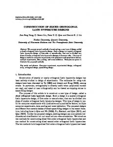
permutation of g18 (1, 2). Obtain the remaining entries of C(:, 1) in a similar fashion. The key idea of Steps 1 and 2 is shown in Table ??. In order the whole design to be a Latin hypercube of 18 runs, it must be a permutation of Z18 for each column, where six entries of each slice must be a permutation of Z6 after level-mapping. To achieve these goals, the construction randomly chooses one entry from each of six g18 (u, v) blocks to form six entries of each slice. For example, C1 (:, 1) in Table ?? (d) has 3, 6, 8, 12, 15 and 18. These six numbers become Z6 after level-mapping dcik /3e, as indicated in numbers in parenthesis in Table ?? (d). Table ?? (d) presents the matrix C with three slices C1 , C2 and C3 divided by the dashed lines. Furthermore, each entry still retains the structure of the underlying OA because all entries in g18 (u, v) become u after levelmapping dcik /6e. Figure 5 presents the bivariate projections of D of 18 runs generated from C. The whole design achieves one-dimensional stratification with respect to the 18 equally spaced intervals of (0, 1] and two-dimensional stratification with respect to the3 × 3 grids displayed in dashed lines. In any one-dimensional projection, each of the 18 equally spaced intervals of (0, 1] contains exactly one point. In any two-dimensional projections, each of the nine reference squares of (0, 1]2 contains exactly two points. The design is divided into three Latin hypercube designs of six runs (#, 4, C), each having exactly one point in each of the six equally spaced intervals of (0, 1].

Proposition 1 presents some space-filling properties of D and its slices. Proposition 1. Consider D with slices D1 , . . . , D s obtained above. We have that (i) the design D achieves two-dimensional stratification with respect to the s× s grids when projected onto any two factors and achieves one-dimensional stratification with respect to


ACCEPTED MANUSCRIPT the n2 equally spaced interval of (0, 1] when projected onto each factor; (ii) each Dm achieves one-dimensional stratification with respect to the 1n equally spaced interval of (0, 1] when projected onto each factor.


Compared with the sliced U design in Proposition 1, a sliced Latin hypercube design (Qian 2012) of the same size can only achieve one-dimensional stratification for the whole design. In Section 1, this difference was illustrated by a comparison of a sliced U design and a sliced Latin hypercube design of 16 runs in Figures 1 and 2, respectively. The sliced U design in Figure 2 is generated from an OA(16, 44 , 2) using the above construction method. The design in Figure 1 does not achieve the Proposition 1 (ii) as some reference squares have no point. This additional stratification leads to improved sampling property compared to sliced Latin hypercube designs as presented in Section 4. The method in Tang (1993) divides Zn2 associated with an OA(n2 , sq , 2) into s groups gn2 (1), . . . , gn2 (s) given by gn2 (u) = {z ∈ Zn2 : dz/n1 e = u, } for u = 1, . . . , s,

(6)

and replaces the u’s in each column with a uniform permutation of the n1 numbers of gn2 (u). For A with index λ = 1 in the above construction, C in (4) is reduced to an ordinary U design in Tang (1993) but the step to divide A. using Lemma 1 is still critical for achieving the uniformity in each slice. If an ordinary U design of n2 runs is randomly divided into s slices of n1 runs, these slices are not guaranteed to achieve attractive uniformity.

4

SAMPLING PROPERTIES

Studying sampling properties of space-filling designs is an important area (Tang 1993; Owen 1994; Loh 1996). In this section, we derive sampling properties of sliced U designs in the context of evaluating a blackbox function f in batches. Let F denote the uniform measure on the unit hypercube


ACCEPTED MANUSCRIPT (0, 1]q and f : (0, 1]q → R be a measurable function with

R

f (x)2 dF < ∞. Express dF as

Qq

k=1

dFk ,

where Fk is the uniform measure of the kth dimension. The continuous ANOVA decomposition (Owen 1994; Loh 1996) of f is f =

X

fu ,

(7)


u∈Q

where Q represents the set of all axes of (0, 1]q . For any u ∈ Q, fu can be defined via  Z  X   fv (x) dFQ/u .  f (x) −

(8)

v⊂u

For the empty set ∅, f∅ denotes the grand mean Z μ= f dF.

(9)

R The variance of f , denoted by σ2 = ( f − μ)2 dF, can be decomposed as XZ 2 fu2 dF. σ =

(10)

|u|>0

Let D be a sliced U design of n2 runs from (4) with s slices D1 , . . . , D s of n1 runs. For m = 1, . . . , s, an estimator of μ in (9) using Dm is μˆ m = n1

−1

n1 X i=1

f xm,i ,

(11)

where xm,i denotes the ith run of Dm . Then a combined estimator of μ is defined by −1

μˆ = s

s X

μˆ m ,

(12)

i=1

using n2 runs of D. For u ∈ Q and r = 1, . . . , q, as in Owen (1994) and He and Qian (2011), let wm,i j (u) = {k ∈ u|cm,ik = cm, jk }. As Owen (1994), define Mm (u, r) =

n1 X n1 X i=1 j=1

1|wm,i j (u)|=r , for m = 1, . . . , s,

(13)


ACCEPTED MANUSCRIPT and M(u, r) =

n2 X n2 X i=1 j=1

1|wi j (u)|=r ,

where wi j (u) = {k ∈ u|αik = α jk }. Theorem 1 gives variance formulas for sliced U designs.


Theorem 1. Suppose that E[ f (x)2 ] is well defined and finite , and f is a continuous function on (0, 1]q . Then for μˆ m in (11) and μˆ in (12) under sliced U designs, as s → ∞ with λ fixed, (i) var (μˆ m ) =

X

|u|≥2

(ii) var (μ) ˆ =

X

|u|≥3

−1 Mm (u, |u|)n−2 1 var[ fu (x)] + o(n1 );

−1 M(u, |u|)n−2 2 var[ fu (x)] + o(n2 ).

Theorem 1 (i) implies that the slices of a sliced U design achieve variance reduction similar to those of sliced Latin hypercube design. Theorem 1 (ii) implies that a sliced U design as a whole achieves a similar degree of variance reduction to an ordinary U design constructed in Tang (1993), P −1 and it is superior to a sliced Latin hypercube design with var (μ) ˆ = |u|≥2 n−2 2 var[ fu (x)] + o(n2 ). For detailed theoretical comparison of sliced U designs, ordinary U designs and sliced Latin hypercube designs, see Proposition 3 of the Supplemental Materials. When a sliced U design is used for running several similar computer experiments (Williams et al. 2009; Storlie and Reich 2011), sampling properties can be modified accordingly as given in the Supplemental Materials.

5

NUMERICAL ILLUSTRATION

In this section, we provide numerical examples to corroborate the effectiveness of the proposed design and the associated theoretical results. The true integral value is obtained by using a very large Latin hypercube design of 106 runs.


ACCEPTED MANUSCRIPT Example 5 (continues=exa:xiu). Consider the ordinary differential equation in (1). Assume the distributions of x1 and x2 are is exp(10) and exp(0.1), respectively. We convert x1 and x2 to Uniform (0, 1] using the inverse cumulative distribution technique. We compute the estimators for μ = μ(t) = E(u(t, x)) and its variability. We compare five methods to generate 11 batches, each of 11 points:


(1) SU: a sliced U design with 11 batches, each being a Latin hypercube design, is constructed by using an OA(121, 113 , 2); (2) IID: 11 IID samples; (3) ILHD : 11 repeated Latin hypercube designs; (4) SLHD: a sliced Latin hypercube designs of 11 slices; (5) OU: a randomly divided ordinary U design into 11 slices. We replicate 1000 times for each method. P ( j) For replicate j, we calculate two estimators for μ: (1) batch estimator: μˆ m( j) = 111 11 i=1 u(t, xm,i ), P for m = 1, . . . , 11; (2) combined estimator: μˆ ( j) = 111 11 ˆ (mj) , and compute batch-to-batch varim=1 μ P ability s( j) = [ 101 11 ˆ m − μˆ ( j) )2 ]−1/2 and sample bias δ( j) = μˆ ( j) − μ. m=1 (μ

Table ?? presents the values of s( j) and δ( j) averaged over the 1000 replicates. Table ?? presents

the sample standard deviation of μˆ ( j) across the 1000 replicates. The sliced U method not only provides the batch-to-batch variability comparable to those from ILHD and SLHD, but also achieve the same small standard deviation of μˆ as the OU method. These dual properties make sliced U designs appealing for both computing UQ values and quantifying the variability of the estimate. The δ( j) results confirm thatˆμ from all the five designs are unbiased. Example 6 (label=ex:borehole). Let f be the borehole function (Morris et al. 1993) given by 2πx3 (x4 − x6 ) 7 x3 + log(x2 /x1 ) 1 + 2 log(x2x/x 2 1 )x x8 1

x3 x5

.

(14)

We compute the estimators for mean μ = E( f (x)) and its variability. A sliced U design with 13 slices, each being a Latin hypercube design, is constructed by using an OA(169, 139 , 2). P ( j) For replicate j, we calculate two estimators for μ: (1) batch estimator: μˆ (mj) = 131 13 i=1 f (xm,i ), P for m = 1, . . . , 13; (2) combined estimator: μˆ ( j) = 131 13 ˆ (mj) , and compute batch-to-batch varim=1 μ P ˆ m − μˆ ( j) )2 ]−1/2 and sample bias δ( j) = μˆ ( j) − μ. ability s( j) = [ 121 13 m=1 (μ


ACCEPTED MANUSCRIPT Table ?? presents the values of s( j) and δ( j) averaged over the 1000 replicates. Table ?? presents the sample standard deviation of μˆ ( j) across the 1000 replicates. The sliced U method not only provides the batch-to-batch variability comparable to those from ILHD and SLHD, but also achieves the same small standard deviation of μˆ as the OU method.


Sliced U designs can also be used to quantifying the uncertainty of a surrogate model fˆ for a complex model f . For replicate j, fit a Gaussian processfˆ using mlegp (Dancik 2011) for evaluating f in (14) on a Latin hypercube design of 50 runs. Then we calculate two estimators P ˆ ( j) for μ: (1) batch estimator: μˆ (mj) = 131 13 i=1 f (xm,i ), for m = 1, . . . , 13; (2) combined estimator: P P μˆ ( j) = 131 13 ˆ (mj) , and compute batch-to-batch variability s( j) = [ 121 13 ˆ m − μˆ ( j) )2 ]−1/2 and m=1 μ m=1 (μ sample bias δ( j) = μˆ ( j) − μ.

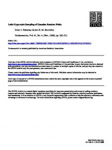
Table ?? presents the values of s( j) and δ( j) averaged over the 1000 replicates. Table ?? presents the sample standard deviation of μˆ ( j) across the 1000 replicates. The sliced U method not only provides the batch-to-batch variability comparable to those from ILHD and SLHD but also achieves the same small standard deviation of μˆ as the OU method. Example 7 (label=ex:datacenter). We use a data center computer experiment from the IT industry that studies the thermal dynamics of an air-cooled data center using Flotherm (Schmidt et al. 2005) to simulate the temperature at a chosen location with a given setting of fixtur es and air control units, as depicted in Figure 6. The response is the temperature at a selected location of the system. The experiment contains five continuous and three categorical factors. Continuous factors are generated from uniform (0, 1], while categorical factors are fixed at one level throughout the simulation. This example is the same spirit of Examples ?? and ?? but using a more complicated surrogate model with real data. Since we do not have access to the resources to re-run the actual model for simulation to compare designs, we use a surrogate model fˆ fitted with 67 runs and the method of Zhou et al. (2011). A sliced U design with 11 slices, each being a Latin hypercube design with 11 runs, is con-


ACCEPTED MANUSCRIPT structed by using the OA(121, 116 , 2). For replicate j, we calculate two estimators for μ: (1) batch P P ( j) estimator: μˆ (mj) = 111 11 ˆ ( j) = 111 11 ˆ (mj) , i=1 f (xm,i ), for m = 1, . . . , 11; (2) combined estimator: μ m=1 μ P ˆ m − μˆ ( j) )2 ]−1/2 and sample bias and compute batch-to-batch variability given by s( j) = [ 101 11 m=1 (μ given by δ( j) = μˆ ( j) − μ.


Table ?? presents the values of s( j) and δ( j) averaged over the 1000 replicates. Table ?? presents the sample standard deviation of μˆ ( j) , across the 1000 replicates. Note that the sliced U method not only provides the batch-to-batch variability comparable to those from ILHD and SLHD, but also achieve the same small standard deviation of μˆ as the OU method.

6

DISCUSSION

We have proposed a new type of space-filling design with an appealing sliced structure. Compared with the proposed designs, existing sliced space-filling designs including Qian and Wu (2009), Sudoku-based space-filling designs (Xu et al. 2011) and those from the infinite (t, s) sequence (Niederreiter 1992; Owen 1995) are constructed by using more complex algebraic methods and are difficult to derive their sampling properties. Sampling properties of our designs are derived for the purpose of estimating the expected output of a computer model, which is a common goal in computer experiments. Sliced U designs have a desirable slicing structure. It will be of interest to explore a similar structure in deterministic points such as Hammersley points (Kalagnanam and Diwekar 1997), or numerical integration (e.g., Lu and Darmofal 2004). These sliced deterministic sequences will have different sample size requirement from sliced U designs, providing complimentary solutions. Multiple computer models are now used to study similar but different physics processes. For example, Hanna et al. (2006) used five computational fluid dynamics models for studying atmospheric flow and dispersion in downtown Manhattan, which employ different assumptions related to state of the flow fields. A computer model often needs to be run multiple times for practical


ACCEPTED MANUSCRIPT reasons. For example, in EnergyPlus, a building energy consumption simulation (Zhang et al. 2013), the properties of glazing materials such as thickness and solar transmittance must be chosen among the available products from the manufacturers, so the model should be run separately for each case. A sliced U design can efficiently allocate computing resources for such a situation.


Multiple machines can be utilized to efficiently run these models with each model associated with one model, especially with potential failures in some batches. There are two advantages for using a sliced U design to run multiple computer models. (1) If the difference between the models is small, the combined design across all slices is space-filling and thus accurately estimates the expected output (over the distribution of all models). (2) If the difference between the models is not small, data from each slice is space-filling and thus accurately estimates the expected output of the corresponding model. This benefit can be supported by the Theorem 1. Sliced U designs are constructed by using existing OAs. Hence, the number of slices and size of each slice are constrained by the chosen corresponding orthogonal array, as pointed out by Tang (1993). Since multiple families of orthogonal array are available (e.g., Chapter 12 of Hedayat et al. 1999), they can be used to construct sliced U designs of different sizes. For example, one can choose OA(50, 55 , 2) to generate a sliced U design of 50 runs, four columns and five slices, or OA(49, 75 , 2) to generate one of 49 runs, four columns and seven slices. When it is computationally infeasible to use all slices, one can take slices in part. The combined slices still have negative dependence between each other, which reduces the variance of the estimator. For example, using ten among 13 slices in Example ?? still performs better than using randomly chosen 130 runs of ordinary U designs. Sliced U designs can also be used to run an expensive code in batches for different nonconnected computers or places. The designs minimize the damage from potential problems caused by machine failure, operational oversight or unexpected delay, while providing the accurate information when every batch is completed and combined. A sliced U design guarantees that if the


ACCEPTED MANUSCRIPT data are shared successfully, the whole design is space-filling. If some batches malfunction or cannot be shared, the sliced structure guarantees that each batch still achieves excellent stratification. Other applications include the computer models with qualitative and quantitative factors, and cross-validation.


When the proposed methods are used for building surrogate models in computer experiments, one may consider constructing sliced U designs according to some distance criterion (Morris and Mitchell 1995). In the writing of this paper, we became aware that Yin et al. (2014) proposed another approach to use orthogonal arrays to construct sliced structured design, but in a different fashion from ours.

ACKNOWLEDGMENT The authors thank David Steinberg for useful discussions, and thank the Editor, the Associate Editor, and three referees for their helpful comments and suggestions, which have led to improvements in the article. Hwang and Qian are supported by NSF Grant DMS-1055214.

References Argonne National Laboratory (2001), User’s Manual for RESRAD Version 6, Argonne National Laboratory, Argonne, Illinois. Bingham, D., Sitter, R. R., and Tang, B. (2009), “Orthogonal and Nearly Orthogonal Designs for Computer Experiments,” Biometrika, 96, 51–65. Dancik, G. M. (2011), mlegp: Maximum Likelihood Estimates of Gaussian Processes, R package version 3.1.2.


ACCEPTED MANUSCRIPT Foo, J. and Karniadakis, G. (2010), “Multi-Element Probabilistic Collocation in High Dimensions,” Journal of Computational Physics, 229, 1536–1557. Hamann, H., van Kessel, T., Iyengar, M., Chung, J. Y., Hirt, W., Schappert, M., Claassen, A., Cook, J., Min, W., Amemiya, Y., Lopez, V., Lacey, J., and O’Boyle, M. (2009), “Uncovering Downloaded by [Academy of Mathematics and System Sciences] at 21:44 04 February 2015

energy-efficiency opportunities in data centers,” IBM Journal of Research and Development, 53, 10:1–10:12. Hanna, S. R., Brown, M. J., Camelli, F. E., Chan, S. T., Hansen, W. J. C. O. R., Huber, A. H., Kim, S., , Reynolds, R. M., and Hansen, Alan H. Huber, R. M. R. (2006), “Detailed Simulations of Atmospheric Flow and Dispersion in Downtown Manhattan: An Application of Five Computational Fluid Dynamics Models,” Bulletin of the American Meteorological Society, 87, 1713–1726. Hansen, C. W., Helton, J. C., and Sallaberry, C. J. (2012), “Use of replicated Latin hypercube sampling to estimate sampling variance in uncertainty and sensitivity analysis results for the geologic disposal of radioactive waste,” Reliability Engineering & System Safety, 107, 139–148. He, X. and Qian, P. Z. G. (2011), “Nested Orthogonal Array Based Latin Hypercube Designs,” Biometrika, 98, 721–731. Hedayat, A. S., Sloane, N. J. A., and Stufken, J. (1999), Orthogonal Arrays: Theory and Applications, New York: Springer. Helton, J. C. and Davis, F. J. (2003), “Latin Hypercube Sampling and the Propagation of Uncertainty in Analyses of Complex Systems,” Reliability Engineering and System Safety, 81, 23–69. Iman, R. L. and Helton, J. C. (1988), “An Investigation of Uncertainty and Sensitivity Analysis Techniques for Computer Models,” Risk Analysis, 8, 72–90.


ACCEPTED MANUSCRIPT Kalagnanam, J. R. and Diwekar, U. M. (1997), “An Efficient Sampling Technique for Off-Line Quality Control,” Technometrics, 39, 308–319. Lin, C. D., Bingham, D., Sitter, R. R., and Tang, B. (2010), “A New and Flexible Method for


Constructing Designs for Computer Experiments,” Annals of Statistics, 38, 1460–1477. Lin, C. D., Mukerjee, R., and Tang, B. (2009), “Construction of Orthogonal and Nearly Orthogonal Latin Hypercubes,” Biometrika, 96, 243–247. Lin, D. K. J. (1993), “A New Class of Supersaturated Design,” Technometrics, 35, 28–31. Loh, W.-L. (1996), “On Latin Hypercube Sampling,” Annals of Statistics, 24, 2058–2080. Lu, J. and Darmofal, D. L. (2004), “Higher-dimensional Integration with Gaussian Weight for Applications in Probabilistic Design,” SIAM Journal on Scientific Computing, 26, 613–624. McKay, M., Conover, W., and Beckman, R. J. (1979), “A Comparison of Three Methods for Selecting Values of Input Variables in the Analysis of Output from a Computer Code,” Technometrics, 21, 239–245. Mease, D. and Bingham, D. (2006), “Latin Hyperrectangle Sampling for Computer Experiments,” Technometrics, 48, 467–477. Morris, M. D. and Mitchell, T. J. (1995), “Exploratory Designs for Computational Experiments,” Journal of Statistical Planning and Inference, 43, 381–402. Morris, M. D., Mitchell, T. J., and Ylvisaker, D. (1993), “Bayesian Design and Analysis of Computer Experiments: Use of Derivatives in Surface Prediction,” Technometrics, 35, 243–255. Niederreiter, H. (1992), Random Number Generation and Quasi-Monte Carlo Methods, Philadelphia: Society for Industrial Mathematics.


ACCEPTED MANUSCRIPT Owen, A. B. (1992a), “A Central Limit Theorem for Latin Hypercube Sampling,” Journal of the Royal Statistical Society. Series B, 54, 541–551. — (1992b), “Orthogonal Arrays for Computer Experiments, Integration and Visualization,” Statis-


tica Sinica, 2, 439–452. — (1994), “Lattice Sampling Revisited: Monte Carlo Variance of Means over Randomized Orthogonal Arrays,” The Annals of Statistics, 22, 930–945. — (1995), “Randomly Permuted (t, m, s)-nets and (t, s)-sequences,” Monte Carlo and Quasi-Monte Carlo Methods in Scientific Computing, Lecture Notes in Statistics , 106, 299–317. Pasanisi, A. and Dutfoy, A. (2012), “An Industrial Viewpoint on Uncertainty Quantification in Simulation: Stakes, Methods, Tools, Examples,” in Uncertainty Quantification in Scientific Computing, eds. Dienstfrey, A. and Boisvert, R., Springer Berlin Heidelberg, vol. 377 of IFIP Advances in Information and Communication Technology, pp. 27–45. Patterson, H. D. (1954), “The Errors of Lattice Sampling,” Journal of the Royal Statistical Society. Series B, 16, 140–149. Qian, P. Z. G. (2012), “Sliced Latin Hypercube Designs,” Journal of the American Statistical Association, 107, 393–399. Qian, P. Z. G., Tang, B., and Wu, C. F. J. (2009), “Nested Space-Filling Designs for Computer Experiments With Two Levels of Accuracy,” Statistica Sinica, 19, 287–300. Qian, P. Z. G. and Wu, C. F. J. (2009), “Sliced Space-filling Designs,” Biometrika, 96, 945–956. Schmidt, R. R., Cruz, E. E., and Iyengar, M. K. (2005), “Challenges of Data Center Thermal Management,” IBM Journal of Research and Development, 49, 709–723.


ACCEPTED MANUSCRIPT Stein, M. (1987), “Large Sample Properties of Simulations Using Latin Hypercube Sampling,” Technometrics, 29, 143–151. Storlie, C. and Reich, B. (2011), “Calibration and Prediction Using Multiple Computer Models,”


in Presenation, The 2011 INFORMS Annual Conference, Charlotte, NC. Tang, B. (1993), “Orthogonal Array-Based Latin Hypercubes,” Journal of the American Statistical Assocation, 88, 1392–1397. Williams, B., Morris, M., and Santner, T. (2009), “Using Multiple Computer Models/Multiple Data Sources Simultaneously to Infer Calibration Parameters,” in Presenation, The 2009 INFORMS Annual Conference, San Diego, CA. Xiu, D. (2010), Numerical Methods for Stochastic Computations, Princeton, New Jersey: Princeton University Press. Xu, H. (2005), “Some Nonregular Designs from the Nordstrom-Robinson Code and Their Statistical Properties,” Biometrika, 92, 385–397. Xu, H. and Wu, C. F. J. (2005), “Construction of Optimal Multi-level Supersaturated Designs,” Annals of Statistics, 33, 2811–2836. Xu, X., Haaland, B., and Qian, P. Z. G. (2011), “Sudoku-based Space-filling Designs,” Biometrika, 98, 711–720. Ye, K. Q. (1998), “Orthogonal Column Latin Hypercubes and Their Application in Computer Experiments,” Journal of the American Statistical Association, 93, 1430–1439. Yin, Y., Lin, D. K., and Liu, M.-Q. (2014), “Sliced Latin Hypercube Designs via Orthogonal Arrays,” Journal of Statistical Planning and Inference, 149, 162–171.


ACCEPTED MANUSCRIPT Zhang, R., Liu, F., Schoergendorfer, A., Hwang, Y., Lee, Y. M., and Snowdon, J. L. (2013), “Optimal Selection of Building Components Using Sequential Design via Statistical Surrogate Models,” in Proceedings of Building Simulation, pp. 2584–2592. Zhou, Q., Qian, P. Z. G., and Zhou, S. (2011), “A Simple Approach to Emulation for Computer Downloaded by [Academy of Mathematics and System Sciences] at 21:44 04 February 2015

Models With Qualitative and Quantitative Factors,” Technometrics, 53, 266–273.



ACCEPTED MANUSCRIPT 1 1 1 2 2 2 3 3 3

1 2 3 1 2 3 1 2 3

1 2 3 2 3 1 3 1 2

1 3 → 2 2 1 3 3 2 1

1 1 1 2 2 3 3 3 2

Table 1: Collecting the three runs of an OA(9, 34 , 2) with 1 in the first column produces an OA(3, 33 , 1).



ACCEPTED MANUSCRIPT

Table 2: (a) An OA(9, 34 , 2) denoted by A, (b) divide A into submatrices A1 , A2 and A3 (indicated by the dashed lines) according to different symbols in column 4 of A and deleting column 4 and randomly shuffle the rows in each slice, (c) C = (cik ) obtained by the construction, where each slice is a Latin hypercube of three runs taking values in Z3 after every entry cik is collapsed according to level-mapping dcik /3e.



ACCEPTED MANUSCRIPT

ACCEPTED MANUSCRIPT

25


ACCEPTED MANUSCRIPT

ACCEPTED MANUSCRIPT

26


ACCEPTED MANUSCRIPT

ACCEPTED MANUSCRIPT

27


ACCEPTED MANUSCRIPT

ACCEPTED MANUSCRIPT

28


ACCEPTED MANUSCRIPT

Figure 1: A sliced Latin hypercube design of 16 runs that is divided into four small Latin hypercube designs of four runs, denoted by #, 4, C, , respectively, where the whole design achieves onedimensional stratification with respect to the 16 equally spaced intervals of (0, 1] and each slice achieves one-dimensional stratification with respect to the four equally spaced intervals of (0, 1].



ACCEPTED MANUSCRIPT

Figure 2: A sliced U design of 16 runs that is divided into four small Latin hypercube designs of four runs, denoted by #, 4, C, , respectively, where the whole design achieves one-dimensional stratification with respect to the 16 equally spaced intervals of (0, 1] and two-dimensional stratification with respect to the 4 × 4 grids, and each slice achieves one-dimensional stratification with respect to the four equally spaced intervals of (0, 1].



ACCEPTED MANUSCRIPT

Figure 3: A design obtained by combining three independent Latin designs of three runs, denoted by #, 4, +, respectively, which does not achieve two-dimensional stratification as some reference squares have no point.



ACCEPTED MANUSCRIPT

Figure 4: An ordinary U design of nine runs that is randomly divided into three slices of three runs, denoted by #, 4, +, respectively, where some slices do not achieve one-dimensional stratification.



ACCEPTED MANUSCRIPT

Figure 5: Bivariate projections of a sliced U design D with slices D1 , D2 and D3 in Example 4. Each of the 3 × 3 squares in the dashed lines has exactly two points, and each of the 18 equally spaced intervals of (0, 1] contains exactly one point. The array D is divided into three Latin hypercube designs of six runs (#, 4, C), each containing exactly one point in each of the six equally spaced intervals of (0, 1].



ACCEPTED MANUSCRIPT

Figure 6: A typical raised-floor data center layout (Hamann et al. 2009).


Technometrics Sliced Orthogonal Array Based Latin Hypercube Designs

Technometrics Sliced Orthogonal Array Based Latin Hypercube Designs

Suggest Documents

Sliced Orthogonal Array Based Latin Hypercube ...

construction of sliced orthogonal latin hypercube designs

Uniform sliced Latin hypercube designs - Wiley Online Library

nearly orthogonal latin hypercube designs for many design columns

a central limit theorem for nested or sliced latin hypercube designs

Fast Generation of Space-Filling Latin Hypercube Sample Designs

Optimizing Latin hypercube designs by particle ... - Semantic Scholar

Space-filling Latin hypercube designs for computer experiments

Nearly Orthogonal Latin Squares

Latin Hypercube Sampling with Evolutionary ... - Semantic Scholar

Latin hypercube sampling with inequality constraints

Latin Hypercube Sampling of Gaussian Random ...

Efficiency Enhancement of Optimized Latin Hypercube Sampling ...

Hierarchical Refinement of Latin Hypercube ... - Semantic Scholar

An Orthogonal Least Squares Based Approach to FIR Designs

Quasi-Latin designs - Project Euclid

Quasi-Latin designs - Project Euclid

Taguchi Orthogonal Array Based - CiteSeerXwww.researchgate.net › publication › fulltext › 25753605

Optical implementation of the weighted sliced orthogonal ... - UV

Signed group orthogonal designs and their applications

Using Cyclotomy to Construct Orthogonal Designs - UOW

ON ADAPTIVE TESTING IN ORTHOGONAL SATURATED DESIGNS

Algebraic generation of Orthogonal Fractional Factorial Designs

Orthogonal designs via computational algebra - Google Sites