Adaptive Load Balancing of Parallel Applications with Multi-Agent Reinforcement Learning on Heterogeneous Systems Johan PARENT, Katja VERBEECK, Ann NOWE, Kris STEENHAUT COMO, VUB Brussels, Belgium Email:
[email protected], {kaverbee, an.nowe, ksteenha}@vub.ac.be Jan LEMEIRE, Erik DIRKX PADX, VUB Brussels, Belgium Email:
[email protected],
[email protected] Submitted for Scientific Programming journal, special issue on Distributed Computing and Computation, IOS Press ABSTRACT We report on the improvements that can be achieved by applying machine learning techniques, in particular reinforcement learning, for the dynamic load balancing of parallel applications. The applications being considered here are coarse grain data intensive applications. Such applications put high pressure on the interconnect of the hardware. Synchronization and load balancing in complex, heterogeneous networks need fast, flexible, adaptive load balancing algorithms. Viewing a parallel application as a one-state coordination game in the framework of multi-agent reinforcement learning, and by using a recently introduced multi-agent exploration technique, we are able to improve upon the classic job farming approach. The improvements are achieved with limited computation and communication overhead. Keywords: Parallel processing, Adaptive load balancing, reinforcement learning, heterogeneous network, intelligent agents, data intensive applications. 1.
INTRODUCTION
Load balancing is crucial for parallel applications since it ensures a good use of the capacity of the parallel processing units. We look at applications which put high demands on the parallel interconnect in terms of throughput. Examples are compression applications which both process important amounts of data and require a lot of computations. Data intensive applications [2] require a lot of communication and are therefore dreaded for most parallel architectures. The problem is exacerbated when working with heterogeneous parallel hardware. This is the case in our experiment using a heterogeneous cluster of PC’s to execute parallel applications with a master-slave software architecture. Adaptive load balancing is indispensable if system performance is unpredictable and no prior knowledge is available [1]. In the multi-agent community, adaptive load balancing is an interesting testbed for multi-agent learning algorithms, likewise for multi-agent reinforcement algorithms as in [9][12]. However the interpretations and models of load balancing there are not always in the view of real parallel
applications. We report on the results obtained by adaptive agents in the farming scheme. The idea is to view all slaves as independent reinforcement learning agents who try to learn the amount of data to request from the master, so as to minimize the total run time of the parallel application and/or the total idle time of the master. As the agents share a common goal, from the game theoretical point of view [10], this setup can be seen as a coordination game. Recently a new exploration technique for individual reinforcement learners used in coordination games was introduced, see [16][17]. This technique allows the slave to learn independently and adaptively which amount of data to request to the master; aiming at an efficient use of the communication link by the group of agents. Our results show that the multi-agent learning technique improves upon the sequential job farming scheme for parallelizing data intensive applications. Section 2 defines the problem of load balancing and gives an overview of the existing load balancing strategies. Section 3 discusses performance metrics, while section 4 introduces reinforcement learning and outlines the multi-agent reinforcement learning algorithm. Section 5 and 6 give the experimental setup and results achieved. Finally some conclusions are drawn in section 7.
2.
LOAD BALANCING/JOB SCHEDULING
Load balancing aims at assigning to each processor an amount of work proportional to its performance, minimizing the execution time of the program. However, processor heterogeneity and performance fluctuations make static load balancing insufficient [1]. We investigate dynamic, local, distributed load balancing strategies [18], which are based on heuristics, since finding the optimal solution has shown to be NP-complete in general [11]. Following the agent philosophy, the request assignment strategy is a receiver-initiated algorithm [6], in which the “consumers” of workload look for producers [13]. The goal is a fast adaptive system that optimizes computation and synchronization. Problem description In situations were the communication time is not negligible, as is the case for data intensive applications, faster processing units can incur serious penalties due to slower units. A data request issued
by a slow unit can stall a faster unit when using farming. This of course results in a reduction of the parallelism. This phenomenon is bound to occur when slaves request identical amounts of data from the master. This is independently of the actual amount by neglecting the communication delay, acceptable given sufficiently large requests. In order to improve upon the job-farming scheme when working with heterogeneous hardware, the slaves have to request different amount of data from the master (server). Indeed their respective consumption of communication bandwidth should be proportional to their processing power. Slower processing units should avoid obstructing faster ones by requesting less data. Computation model The initial computation model is job farming. In this master-slave architecture the slaves (one per processing unit) request a chunk of a certain size from the master. As soon as the data has been processed the result is transferred to the master and the slave sends a new request (figure 1).
( 1) Overhead = T par . p − Ts . Hence, the choice of speedup as the performance measure implies means that each processor has Tpar time allocated to perform its part of the job: 1 2 p T par = T par = T par = ... = T par . ( 2) i i i, j Tpar = Tcomp + ∑ T overhead .
( 3)
j
With
i the time that processor i performs its part T comp
wi of the total useful work W and
i, j the time T overhead
not overlapped with the computation of the overhead of type j. To study the overall impact of the overhead, we can rewrite Eq. (2) as
∑T
Tpar =
i par
i
p
.
( 4)
We will develop the overhead equations for homogeneous processors (with equal computing power) which implies that i Tseq = ∑ Tcomp .
( 5)
i
master communication bottleneck
1. request chunk
Together with Eqs. (3) and (4), the speedup can then be rewritten as:
S=
4. send result
1+
2. send chunk
slave 1 3. data crunching
slave 2
slave p heterogeneous processors
3.
PERFORMANCE METRICS
We quantify the benefit of parallel processing by the speedup S=Tseq/Tpar, how much faster the parallel program runs with respect to the runtime of the sequential version. The portion of Tpar that is not used for useful computation is therefore as considered lost processor cycles [4], or overhead:
i
( 6)
j
Tseq
The impact of the overhead on the speedup is thus reflected by its ratio with the sequential runtime. Let us therefore define this ratio for each overhead type j:
Fig 1: Model. This scheme has the advantage of being both simple and efficient. Indeed, in the case of heterogeneous hardware, the load (amount of processed data) will depend on the processing speed of the different processing units. Faster processing units will more frequently request data and thus be able to process more data. The bottleneck of data intensive applications with a master-slave architecture is the link connecting the slaves to the master. In the presented experiments all the slaves share a single link to their master (through an ethernet switch). In this scenario the application’s performance will be influenced by the efficient use of the shared link to the master. Indeed, the fact that the application has a coarse granularity only ensures that the computation communication ratio is larger than one. But it does not preclude a low parallel efficiency even when using job farming.
p . i, j ∑∑ T overhead
Ovh = j
j T overheads
Tseq
. ( 7)
These ratios quantify the cost of the overheads. Note that
j T overhead
is the summation of that type of
overhead over all processors i. Heterogeneity Let us have a look how system heterogeneity affects the performance. For different computing powers, we introduce the relative speed ppi, measured with respect to a reference machine:
ppi =
Tcomp (W ) i Tcomp (W )
( 8)
Unlike most works on heterogeneous parallel systems [19], we express the speeds relatively to a fixed machine [3], and not relatively to the fastest processor. We think that choosing a fixed reference, with which the sequential runtime Tseq is measured, allows a clearer performance analysis. Equation (5) is based on the assumption that the runtime does not depend on a particular portion of the work. Similarly, we assume that the various processors essentially differ in their clock speed [3] and not in the size of the task. The total relative processing power of the parallel system is then:
PP = ∑ ppi
( 9)
i
For a heterogeneous system, the efficiency is the performance compared with the ideal performance, namely PP:
E=
S PP
( 10)
pp =
With the average relative speed
PP p
we
define the degree of heterogeneity H of a parallel system by the standard deviation of ppi [3]:
∑ ( pp − pp )
2
i
H=
i
( 11)
p
To continue the performance analysis of the previous paragraph, Eq. (5) should be replaced by i Ts = ∑ ppi .Tcomp
( 12)
i
Also for the calculation of the overhead ratio Ovhj (Eq. 7),
i, j Toverhead should be scaled with ppi
Ovh = j
∑ pp .T i
i, j overhead
i
( 13)
Tseq
Thus, we can conclude that all time measurements on a processor should be scaled with ppi. Slower processors will carry out less useful work in a given time and the parallel overheads will have less impact on the speedup. This result corresponds with the approach proposed in [4], which essentially uses processor cycles as time unit.
where qop is the number of operations per quantum work and τ represents the atomic computing time per ‘operation' on the reference machine. However, a piece of code cannot be divided in equal operations, τ should be considered a reference computing time. It is the product qop..τ, the length of a run-time quantum, that we will use and that we considered to be constant. We then define the granularity as a relative measure of the amount of computation with respect to the amount of communication within a parallel algorithm implementation [14]:
gran =
Tcomp Tcomm
=
1 τ qop = . Ovhcomm β qdata
It depends on hardware and software, so τ called the hardware granularity and qop
qdata
( 16) is
β
the
software granularity. The performance is affected by the overall granularity, independent of how the granularity is spread over software and hardware. We define gran as the granularity measured on the reference machine and grani the granularity of processor i. Since the communication time is fixed, the granularity of each processor is
grani = gran. ppi
( 17)
Load balancing equilibrium
Granularity In load-balancing problems, the overheads are mainly communication and idle time, that we call blocking overhead. In our setting, the learning algorithm can only improve the performance by minimizing blocking, since the communication time represents the lower bound. Moreover, the communication overhead is proportional with the total data size of the work. For data-intensive applications with large messages, all other contributions to the communication time, like the latency or delay, can be neglected. The total work consists of W quantums, where each quantum processes an amount of qdata bytes, the communication time becomes
Tcomm = β .qdata .W
( 14)
where β is the time to transmit a byte from the master to any slave. We assume it to be constant, as we do not consider heterogeneous communication networks. In the same way, the computation time can be expressed as a function of the work W by a first order equation. In this equation the linear term is the main contribution, especially for linear data-intensive applications that we consider. The computation time becomes
Tcomp = τ .qop .W
(2a)
( 15)
(2b) Fig 2: Load balancing with a clear computation bottleneck. Execution profile(a) and overhead distribution (b)
W
∑ w = ∑ 1 + gran i
i
i
=W
( 21)
i
This results in the load balancing equilibrium condition, which indicates a match between the systems communication bandwidth and processing power
1
∑ 1 + gran i
=1
( 22)
i
We introduce the load balancing equilibrium factor lbe to quantify this match
lbe = ∑ i
Fig 3: Load balancing with a clear communication bottleneck. Execution profile(a) and overhead distribution (b) We will investigate the non-trivial case of load balancing where the total computation power of the slaves matches the communication bandwidth of the master for a given total granularity. In other cases, there will be either a clear communication or computation bottleneck, what makes adaptive load balancing unnecessary. Indeed, with a total computation power that is lower than the master’s communication bandwidth, there is no bottleneck, the master will be able to serve the slaves constantly and these will work at 100% efficiency. This can be seen in the experiment of figure 2, where the total computation power is lower than the communication bandwidth. In that case, more processors can be added to increase the speedup. On the other hand, when the total computation power increases, the master will get requests at a higher rate and the communication becomes the bottleneck. Then, the slaves will start to block, waiting to be served and their efficiency drops. This can be seen in figure 3, where the total computation power is higher than the communication bandwidth. In that case, the surplus of slave processors should better be used for other work. In both cases, the distribution of the work can hardly be optimized. We will investigate the non-trivial case, when computation and communication speed match. In that case, workload assignment and synchronization becomes necessary. At the equilibrium point, an ideal load distribution exists, so that the master can serve the slaves constantly and these are fully busy. There will be no blocking on master or slaves, so their parallel runtime is 1 Tpar = B.W
( 18)
i i i Tpar = Tcomm + Tcomp = B.wi + grani .B.wi (i > 1)
( 19) Where grani is the granularity of processor i. Since all parallel runtimes are equal (Eq. (2)), Eq. (18) equals Eq. (19) and wi can be calculated for each slave
wi =
B.W W = B.(1 + grani ) 1 + grani
( 20)
We know that W is the summation of all wi, hence
1 1 + grani
( 23)
Where lbe=1 reflects an equilibrium, lbe < 1 is for lower processing power (Fig 2, where lbe=0.5) and lbe > 1 indicates a communication bottleneck (Fig 3, where lbe=2) For a homogeneous system, grani is constant for all processors, and according to Eq.(22), the equilibrium condition becomes p = gran + 2 and the speedup is then S = p − 2 . Note that p should be greater than 2, we need at least 2 slaves, so that one can compute when the other communicates. The load balancing equilibrium factor is then
lbe = 4.
p −1 1 + gran
( 24)
MULTI AGENT REINFORCEMENT LEARNING
Reinforcement learning (RL) is the problem faced by an agent that learns behavior through trial-and-error interactions with a dynamic environment. A model of reinforcement learning consists of a discrete set of environment states, a discrete set of agent actions and a set of scalar reinforcement signals. For each interaction the agent receives reinforcement and the next state of the environment, and chooses an action. The agent's job is to find a policy, i.e. a mapping from states to actions, which maximizes some long-turn measure of reinforcement. These rewards can take place arbitrarily far in the future. To obtain a high overall reward, an agent has to prefer actions that it has learned in the past and found to be good, i.e. exploitation, however discovering such actions is only possible by trying out alternative actions, i.e. exploration. Neither exploitation, nor exploration can be pursued exclusively. In our load-balancing problem setting processors are of the receiver-initiated type and can thus be viewed as agents, which we will give extra learning abilities. Each processor will be an independent RL agent, which tries to learn an optimal chunk size of data to ask the master, so that the blocking time for others is minimized and therefore also the total computation time. The agents’ actions are the possible amounts of data or block sizes available. Because we want to restrict ourselves to reinforcement learners with a discrete set of actions, we specify at the beginning a set of possible block sizes the agents can choose
from. Since there are multiple slaves existing together, which influence each other, we have to use a multi-agent reinforcement learning scheme. In our application, the slaves can only be in one state and they share a common goal. As such this multi-agent problem can be viewed as a coordination game, in which the agents should learn to converge to the Pareto Optimal Nash equilibrium1 of the game. In [17] an algorithm for learning in a multi-agent coordination game is given. We describe it in short in the next subsection. Exploration in a multi-agent coordination game The learning scheme starts with a number of exploration periods and is followed by an exploitation phase. At the beginning of each exploration period, agents behave selfish and naive; i.e. they ignore the other agents in the environment and use some traditional reinforcement learning technique to maximize their payoff. The exploration period ends when the agents have found a Nash equilibrium. This will happen because it is assured by results from Learning Automata theory [8] and also holds for other reinforcement learning algorithms such as Q-learning [7][15]. Which Nash equilibrium the agents find is not known in advance, it depends on the initial conditions and the basin of attraction of the different equilibriums. The goal is to converge to the best Nash equilibrium, i.e. the Pareto Optimal equilibrium. After having converged, every agent will exclude its last action played, so that the joint action space becomes considerable smaller. In a new period of play, a new Nash equilibrium will be found. Before a new period starts, the agent keeps some statistics for the action it has converged too. When the agent has no actions left, its original action space is restored. New exploration periods are played until the user decides to stop the exploration phase and decides to exploit the best Nash equilibrium found. This is achieved without any communication between the agents, because they sense the same payoff for each joint action played. The joint action they choose after exploration is the best they have seen so far. Under some assumptions concerning period-length and number of periods played, convergence to the Pareto Optimal equilibrium is assured, even for stochastic rewards/payoffs see [17]. In the next subsection we explain how to use this multi-agent learning algorithm in the load balancing experiment, which can be viewed as an asynchronous version2 of a coordination game. 5.
EXPERIMENTAL SETUP
1 An outcome of a game is said to be Pareto Optimal if there exists no other outcome, for which all the players simultaneously do better. A Nash equilibrium of a game is a solution for which no agent can do better by changing his policy, as all the other keep playing their Nash equilibrium policy [10]. 2 Asynchronous in the sense that players do not take their actions synchronously, rewards may be delayed etc.
To assess the presented algorithm for coarse grain data intensive applications on heterogeneous parallel hardware a synthetics approach has been used. An application has been written using the PVM [5] message-passing library to experiment with the different dimensions of the problem. The application has been designed not to perform any real computation, but instead it replaces the computation and communication phases by delays with equivalent duration3. For the experimental setup, H and lbe are 2 experiment parameters. H and lbe are set to 1 in all experiments. The granularity of the processors will then be chosen randomly according to a normal distribution with
average =
p −1 − 1 , derived cce
from the homogeneous case granularity, Eq. (24), and stddev = H . This guarantees the experiment to be in an interesting load balancing equilibrium. Learning to request data In our load balancing setting, the slaves use a reward-inaction learning automata scheme for selfish play during the exploration periods [8]. A learning automaton describes the internal state of an agent as a probability distribution according to which actions should be chosen. These probabilities are adjusted according to the success or failure of the actions taken. The update scheme we will use here is the reward-inaction update scheme, given in equation (25). A constant reward parameter a between 0 and 1 is used to reinforce good actions. The feedback r gives the reinforcement from the environment. For this scheme it is proven that players will converge to a Nash equilibrium when it is used in a one-state coordination game, see [8].
pi (n + 1) = pi (n) + a.r (n).(1 − pi (n)) if action i was chosen at time n
p j (n + 1) = p j (n) − a.r (n). p j (n) for all actions j different from i
( 25)
The feedback r provided to the learner is the inverse blocking time, which is the time a slave has to wait before the master acknowledges its request for data. It is used to update the action probabilities by Eq.(25). Less interesting actions will incur higher blocking times and thus will have lower probability associated with them. In our experiment, the slaves will learn to request a chunk size that minimizes its blocking time. To that end each slave has a stochastic learning automaton which uses Eq.(25), as shown in Fig 4. In the presented results the block size is a multiple of a given initial block size. Here the multiples are 1, 2 and 3 … times the initial block size
3
The experimental application can easily be turned into a real application by replacing the delay producing code with real code.
Chunk size
P
S1
P1
S2
P2
S3
P3
random choice of Si ~ Pi
feedback: 1/blocktime
maximally exploited. request Si blocking comm & comp of Si
Fig 4: Reinforcement learning during an exploration period. At the end of an exploration period the slaves have converged to a Nash equilibrium, i.e. each slave has learnt a block size to ask the master. They send to the master their average performance during this period, which is the average amount of data each was able to compute. When the master has received this message from each slave, the overall reward, is sent back to each slave, which uses this to update its statistics for the action last played. The overall reward the agents receive for the joint action played is given by the total average amount of data the agents computed in parallel during the period of play. This payoff can easily be attached to the data packages the master sends to its slaves, no extra communication is generated. The same argument goes for the slave sending period information to the master. The number of exploration periods is chosen in advance. After all periods have been played, the slaves chose the action which was rewarded best by the master. We will compare our adaptive algorithm with a static load-balancing scheme where fixed amounts of data are requested. 6.
EXPERIMENTS
Figure 5 shows the time course of a typical experiment in its exploitation period with the computation, communication and blocking phases. (data size = 10GB, communication speed = 10MB/s, #slaves=3, average chunk size =1MB, H=1, lbe=1, the length of the exploration period = 100s and the number of periods = 10)
Performance results As shown in table 1, we have run several experiments with varying joint action spaces (JAS). We use up to 7 slaves with each 5 possible actions, which results in a joint action space with 57 possibilities. The 4th column gives the absolute gain in total computation time for the adaptive multi-agent algorithm compared to the total computation time for the farming algorithm. The 5th column gives the gain in total computation time which is maximal possible for the given setting. The total computation time can only decrease when the idle time of the master is decreased. No gain is possible on the total communication time of the data. Therefore the last column gives the absolute gain compared to the gain which was maximal possible. In all experiments considerable improvements were made. Agents are able to find settings in which the faster slave is blocked less than the others, see also Fig. 5. The adaptive characteristic of the agents makes them able to take their heterogeneity into account. In larger joint action spaces the gain drops, but by adjusting the parameters of the learning algorithm, i.e. making sure the agents can explore more by enlarging the exploration periods length and increasing the number of exploration periods, performance gets better again in the last experiments. The data size increased from 10 to 30 GB in larger joint action spaces, the period length from 100 to 200 time steps and the number of periods from 10 to 20. All the other settings were taken as above. The figures shown are averaged results for 10 runs of each experiment. Slaves
Actions
#JAS
2 2 2 3 3 5 5 7 7
3 4 5 3 5 3 5 3 5
9 16 32 27 125 243 3125 2187 7812 5
abs. gain (%) 8.40 8.32 6.64 4.69 4.33 1.39 1.61 2.40 3.47
max. gain (%) 13.54 13.54 13.54 14.14 14.14 13.13 13.12 12.20 14.20
rel. gain (%) 62.00 60.99 49.02 33.17 30.65 10.60 12.24 16.91 24.42
Table 1: Average gain in total computation time for adaptive load balancing compared to static load balancing (farming). Fig 5: Execution profile of the exploitation phase of a typical experiment with 3 slaves We observe that the slaves have learned to distribute the requests nicely and hence use the link with the master efficiently. Slave 3, which is the fastest processor with lowest granularity, is served constantly and has no blocking time. Slave 2 has some blocking time. However, it is the slowest processor, so the processing power of the system is
Table 2 shows the results for uniform load balancing. In the uniform version, instead of each agent learning the best amount of chunk size to ask out of a given set of possible sizes, the agents will now choose each possible chunk size with a uniform distribution. Results show that uniform play is on average comparable to static load balancing. So, our learning approach performs better than both.
Slaves
Actions
#JAS
2 2 2 3 3 5 5 7 7
3 4 5 3 5 3 5 3 5
9 16 32 27 125 243 3125 2187 78125
abs. gain (%) 1.32 -1.41 -1.30 -0.87 -1.48 -1.61 -1.78 1.01 0.84
max. gain (%) 13.54 13.54 13.54 14.14 14.14 13.13 13.12 14.20 14.20
rel. gain (%) 9.71 -10.41 -9.56 -6.12 -10.44 -12.28 -13.59 7.11 5.89
Table 2: Average gain in total computation time for uniform load balancing compared to static load balancing (farming). Overhead Analysis Table 3 gives an overview of the gain in blocking overhead. The blocking time represents the cumulated blocking time of all the slaves during the parallel run, the idle time is the idle time of the master. The numbers presented here are averaged over 10 independent runs. Initially a parallel run (using job farming) with 3 slaves which can use 3 different block sizes resulted in an average of 165.27 seconds of idle time for the master. However, when learning is used the idle time of master reduces to 115.08 seconds, a gain of 30.37%. The gain in blocking time follows the same interpretation. Slaves Actions 2 2 2 3 3 5 5 7 7
3 4 5 3 5 3 5 3 5
Idle (gain) 55.6% 54.3% 47.7% 30.3% 26.8% 4.0% 0.98% 9.70% 11.6%
Blocking (gain) 50.7% 51.3% 38.7% 20.7% 20.7% -3.4% 3.20% 3.00% 3.00%
Table 3: Average gain for adaptive load balancing in idle time of the master and total blocking time of the slaves. As shown the task of reducing the blocking time becomes harder as the number of slaves increases. This is a direct result of the exponential increase in size of the search space. 7.
CONCLUSIONS
Complex, heterogeneous system controlled for optimal use by multi-agent reinforcement learning is promising. We implemented reinforcement learners for distributed load balancing of data intensive applications. Together they use a novel technique of coordinated exploration, which was already tested and proven to convergence to the Pareto Optimal
Nash equilibrium in stochastic coordination games from game theory. The master-slave setup we used for our load balancing experiments was viewed as an asynchronous coordination game. Results show that the multi-agent algorithm used still works for asynchronous games. The first performance results show considerable improvements upon a static load balancer. The agents are able to find settings in which the faster slave is less blocked during communication with the master than the others. The adaptive characteristic of the agents makes them able to take their heterogeneity into account. Even more when a slave is removed from the set-up, the remaining agents can adjust themselves tot the new situation. The algorithm works locally on the slaves (receiver-initiated), thus acting like intelligent agents. The agents use both local and global information in their learning process, however no extra communication is needed in-between the slaves to achieve this global information. Every agent communicates its period-performances to the master, which in turn will send the global information back to every slave. This extra information can be attached to the global data packages and requests, without causing extra overload. We are planning to use this multi-agent approach for data intensive applications such as compression applications. 8.
REFERENCES
[1] I. Banicescu and V. Velusamy, “Load Balancing Highly Irregular Computations with the Adaptive Factoring”, Proceedings of the 16th International Parallel & Distributed Processing Symposium, IEEE, Los Alamitos, California, 2002. [2] M. D. Beynon, T. Kurc et al. “Efficient Manipulation of Large Datasets on Heterogeneous Storage Systems”, Proceedings of the 16th International Parallel & Distributed Processing Symposium, IEEE, Los Alamitos, California, 2002. [3] Clematis, A. and Corana, A., “Modeling performance of heterogeneous parallel computing systems”, In Parallel Computing 25, Elsevier Science, 1999. [4] Crovella, M. E. and Leblanc, T.J., “Parallel Performance Prediction using Lost Cycles Analysis”, in Proc. of Supercomputing ’94, IEEE Computer Society, 1994. [5] A. Geist, A. Beguelin et al., “PVM: Parallel Virtual Machine”, the MIT press, 1994. [6] D. Gupta and P. Bepari, "Load sharing in distributed systems", In Proceedings of the National Workshop on Distributed Computing, January 1999. [7] Kaelbling L.P., Litmann M.L., Moore A.W.,: Reinforcement Learning: A Survey. Journal of Artificial Intelligence Research 4 (1996) p 237-285. [8] Narendra K., Thathachar M., “Learning Automata: An Introduction”, Prentice-Hall (1989). [9] Nowé, A., Verbeeck, K., “Distributed Reinforcement learning, Loadbased Routing a case study”, Proceedings of the Neural, Symbolic and Reinforcement Methods for sequence Learning
Workshop at ijcai99, 1999. [10] Osborne J.O.,Rubinstein A., “A course in game theory”, Cambridge, MA: MIT Press (1994). [11] C.C. Price and S. Krishnaprasad, “Software allocation models for distributed systems”, in Proceedings of the 5th International Conference on Distributed Computing, pages 40-47, 1984. [12] Schaerf A., Shoham Y., Tennenholtz M., “Adaptive Load Balancing: A Study in Multi-Agent Learning”, Journal of Artificial Intelligence Research (1995) 475-500. [13] T. Schnekenburger and G. Rackl, “Implementing Dynamic Load Distribution Strategies with Orbix”, International Conference on Parallel and Distributed Processing Techniques and Applications (PDPTA'97), Las Vegas, Nevada, 1997. [14] Stone H.S., 1993. High-Performance Computer Architecture, Addison-Wesley, Massachusetts, 1993. [15] Sutton, R.S., Barto, A.G., “Reinforcement Learning: An introduction”, Cambridge, MA: MIT Press (1998). [16] Verbeeck, K., Nowé, A., Lenaerts T., Parent, J., “Learning to reach the Pareto Optimal Nash Equilibrium as a Team”, LNAI 2557- Proceedings of the 15th Australian Joint Conference on Artificial Intelligence. Pp 407- 418 (2002). [17] Verbeeck, K., Nowé, Tuyls, K.,”Coordinated Exploration in Stochastic Common Interest Games”, Third symposium on Adaptive Agents and Multi-agents Systems, AAMAS-3. (2003) [18] M.J. Zaki, Wei Li; S. Parthasarathy, “Customized dynamic load balancing for a network of workstations”, Proceedings of the High Performance Distributed Computing (HPDC'96), IEEE, 1996. [19] X. Zhang, Y. Yan, “Modeling and characterizing parallel computing performance on heterogeneous networks of workstations”, in Proc. of the 7th IEEE Symposium on Par. And Distr. Proc., IEEE, 1995.