Temporal variability in snow distribution

Temporal variability in snow distribution

Eli Alfnes, Liss M. Andreassen, Rune Engeset, Thomas Skaugen and Hans-Christan Udnæs E-mail: [email protected] Norwegian Water Resources and Energy Directorate (NVE)

1. Introduction

3. Time variant snow distribution function

Snow distribution changes during the winter due to spatially variable snowfall and snowmelt events and wind-induced redistribution of the snow. This influences the spatial distribution of the melting process and thus the dynamics of the spring flood. Snow course data was collected in the catchments Aursunden and Atnasjø during the melt season in order to investigate the temporal variability of the snow distribution in alpine and forested terrain. A time variant gamma distribution function was fitted to the snow course data.

A time variant gamma distribution function

Location map of the catchments Aursunden and Atnasjø, Norway.

0.0

500 1000 1500

2.0

1.0

CV

1.5

0.5 0.0

500 1000 1500

2.0

CV

1.5 1.0 0.5 0.0

1.0 0.0

0.2

0.4

0.6

0.8

1.0 0.8 0.6 0.4

Week 15

0.2 0.0

0

500 1000 1500 Snow water equivalent (mm)

2000

0


2000

0.8

1.0

1500

0.0

0.2

0.4

0.6

0.8

1.0

0.0

0.2

0.4

0.6

0.8 0.6 0.4 0.2 0.6

0.8

1.0

0.0

Week 18

1.0

2000

500 1000 Snow water equivalent (mm)

Atnasjø Forest

(α α=0.0070, ν =0.0233)

(α α=0.0321, ν =0.1070) 0.8 0.0

0.2

0.4

0.6

0.8 0.6 0.4 0.2 0.0

Week 15

1.0

Alpine

2000

0


2000

0

100 200 300 400 Snow water equivalent (mm)

500

0


500

0.8 0.0

0.2

0.4

0.6

0.8

1.0


1.0

0

Conditional empirical CDF’s (cumulative density function) and theoretical gamma (nν=shape, α=rate) CDF for the cathments Aursunden and Atnasjø spring 2002. ▬ Theoretical Gamma CDF. ─ ─ Empirical CDF .


Syndre Langsvola 11 April 2002

0


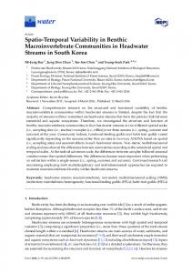
• The spatial distribution of SWE was positively skewed in alpine terrain at snow maximum whereas it was normally distributed in forested terrain. • The skewness increased during the melt season for both terrain types.

At-5

At-4

At-3

At-2

At-1

Au-9

Au-11

Au-8

Au-10

Au-7

Au-6

Au-5

Au-4


0

4. Conclusions 0

0.0 0.2 0.4 0.6 0.8 1.0

0.5

0.0 0.2 0.4 0.6 0.8 1.0

The recorded SWE (snow water equivalent) revealed a large variability of the mean and standard deviation for the various snow courses. Generally, the snow courses in forest (green markers) had a lower CV (coefficient of variation, red line) than those in alpine terrain (blue markers). The variability of the snow cover increased during the melt season.

CV

1.0

Au-3

0

1.0

A distribution function for new areas can be determined by knowing the mean daily precipitation.

CV

1.5

Au-2

2000

0.6

ν was derived assuming that the mean daily precipitation, for days with precipitation, is equal to the expectation value of a unit snowfall, E(y)=ν/α.

2.0

Au-1


0.4

• Three field campaigns during the melt season 2002 (weeks 15, 18 and 21).

0

SWE (mm) Week 15

0

0.2

• Two density samples at each snow course

• 800 - 1200 m a.s.l.

0

Week 18 SWE (mm)

2000

α was calculated by averaging the αvalues for the snow courses in each of the terrain classes, alpine and forest.

Week 18

• Four field sites

0

SWE (mm) Week 21


0.0

• Snow depth every 10 m

500 1000 1500

• Sixteen snow courses

Snow water equivalent for the various courses. /mean value (alpine blue, forest green), × median, ┬/┴ standard deviation, ▬ CV (coefficient of variation). Zero values are excluded from the statistics.

Syndre Langsvola 2 May 2002

1500 1000

SWE Au-4 (mm)


500

1500 1000 500

0

0

0

SWE Au-10 (mm)

Forest

b

• A two parameter gamma distribution was found to give an appropriate description of the temporal changes in the SWE.

0.0 0.2 0.4 0.6 0.8 1.0

Alpine

a

-3

-2

-1

0

1

2

3

-3

-2

Quantiles of Standard Normal

0

1

2

3

600 400

SWE At-1 (mm)

400

Syndre Langsvola 21 May 2002

Snow distribution at Syndre Langsvola, Aursunden.

0

200

600

800

800

d

200

SWE At-4 (mm)

-1


c

0

The alpine courses revealed a positively skewed distribution whereas the forested snow courses followed an approximately normal distribution at snow maximum. A change towards more skewed distributions was observed for both terrain classes as snow melt proceeded.

0

0.4

Atnasjø

(α α=0.0321, ν =0.0787)

0.2

Aursunden

Week 21

was found to represent the observed snow courses well. The scale parameter (α) is a global value for each terrain class, and the shape parameter is expressed as a terrain and catchment dependent constant (ν) multiplied with a variable representing the accumulated number of snow equivalents (n) in the snowfalls and melting events.

2. Snow course data

SWE (mm)

α , nν , y > 0

Forest

(α α=0.0070, ν =0.0233)

0.0

1 f α , nν ( y ) = α nν y nν −1e −αy Γ ( nν )

Aursunden Alpine

-3

-2

-1

0

1


2

3

-3

-2

-1

0

1

2

3


Quantile-Quantile plot of the empirical distribution at snow maximum versus standard normal distribution. Snow courses from the two catchments - Aursunden a) alpine and b) birch forest, and Atnasjø c) alpine and d) pine forest.

SnowMan

5. Current work Field campaigns have also been carried out in 2003. Preliminary analyses of the field observations indicate good agreement with the proposed distribution function.