Testing and Model-Checking Techniques for Diagnosis - Eindhoven

Testing and Model-Checking Techniques for Diagnosis Maxim Gromov1 and Tim A.C. Willemse2 1

Institute for Computing and Information Sciences (ICIS) Radboud University Nijmegen – The Netherlands 2 Design and Analysis of Systems Group, Eindhoven University of Technology – The Netherlands

Abstract. Black-box testing is a popular technique for assessing the quality of a system. However, in case of a test failure, only little information is available to identify the root-cause of the test failure. In such cases, additional diagnostic tests may help. We present techniques and a methodology for efficiently conducting diagnostic tests based on explicit fault models. For this, we rely on Model-Based Testing techniques for Labelled Transition Systems. Our techniques rely on, and exploit differences in outputs (or inputs) in fault models, respectively. We characterise the underlying concepts for our techniques both in terms of mathematics and in terms of the modal µ-calculus, which is a powerful temporal logic. The latter characterisations permit the use of efficient, off-the-shelf model checking techniques, leading to provably correct algorithms and pseudo decision procedures for diagnostic testing.

1 Introduction Testing has proved to be a much-used technique for validating a systems behaviour, but in itself it is a quite labour-intensive job. Formal approaches to testing, collectively known as Model-Based Testing, have been touted as effective means for reducing the required effort of testing by allowing for automation of many of its aspects. However, MBT provides only a partial answer to the validation problem, as in most cases its automation ceases at the point where a test failure has been detected; pinpointing the root-cause of the test failure remains a laborious and time-consuming task. Finding this root-cause is known as the diagnosis problem, and it is tightly linked to testing. Formal approaches to the diagnosis problem rely on the use of models of the systemunder-diagnosis, and are often referred to as Model-Based Diagnosis techniques. While MBD has been studied extensively in the formal domain of Finite State Machines (see e.g. [4, 5, 9, 15]), the topic is little studied in the setting of Labelled Transition Systems. The advantage of many LTS-based theories over FSM-based theories is that the assumptions under which they operate are more liberal, which makes them easier to apply in practice. In this paper, we advocate an LTS-based MBD approach for non-deterministic, reactive systems. The techniques that we put forward in this paper operate under the liberal LTS-based testing hypothesis of ioco-based testing [17]; our methods rely on explicit models describing the faulty behaviour, henceforth referred to as fault models. The problem that we consider consists of identifying “correct” fault models among a given (but large) set of possible fault models. By “correct”, we understand that no

evidence of a mismatch between the malfunctioning system and the fault model can be found. This can be asserted by e.g. testing. Note that even though this problem is readily solved by testing the malfunctioning system against each fault model separately, this is a daunting task which is quite expensive in terms of resources, even when fully automated. The main contributions of this paper are twofold: 1. inspired by classical FSM-based diagnosis approaches we present diagnostic concepts and techniques to make the fault model selection process more effective in an LTS-based setting. In particular, we adopt and modify the notion of distinguishability (see e.g. [15]) from FSMs to fit the framework of LTSs. Secondly, we introduce a novel notion, called orthogonality which helps to direct test efforts onto isolated aspects of fault models. Both notions are studied in the setting of ioco-based testing. 2. we link our diagnostic concepts and techniques to model-checking problems. This gives rise to effective and provably correct automation of our approach, and leads to a better understanding of all involved concepts. Note that the problem of constructing the set of fault models is left outside the scope of this paper; in general, there are an infinite number of fault models per implementation. While this is indeed a very challenging problem, for the time being, we assume that these have been obtained by manually modifying e.g. a given specification, based on modifications of subcomponents of the specifications. Such modifications can be driven by the observed non-conformance between the specification and the implementation, but also fault injection is a good strategy. Related work. In [11], J´eron et al paraphrase the diagnosis problem for discrete event systems (modelled by LTSs), as the problem of finding whether an observation of a system contains forbidden sequences of actions. Their approach takes a description of the structure of a system as input; the sequences of forbidden actions are specified using patterns. They subsequently propose algorithms for, a.o., synthesising a diagnoser which tells whether or not a pattern occurred in the system. A variation on this approach is given in [13], in which all actions are unobservable except for special “warning” actions. The problem that is solved is finding explanations for the observations of observed warning actions. Both works view the diagnosis problem as a supervisory problem. Apart from the above mentioned works in the setting of LTSs, there is ample literature on diagnosis based on FSMs. Guo et al, in [9] focus on heuristics for fault diagnosis, which helps to reduce the cost of fault isolation and identification. El-Fakih et al [5] define a diagnostic algorithm for nets of FSMs, and in [4] these techniques are extended; the effectiveness of (a minor modification of) that algorithm is assessed in [7]. Most FSM-based approaches consist of two steps, the first step being the generation of a number of candidate fault models (often referred to as candidates), and the second step being a selection of appropriate candidates. The first step relies on strict assumptions, which in general are not met in an LTS-based setting. Closely related to our are [1, 14]. In [1] Alur et al raise the problem of state identification in complete non-deterministic FSM. This problem coincides with the problem of identifying a given FSM among a set of non-deterministic FSMs. They rely on a preset distinguishing strategy and an adaptive distinguishing strategy for solving the state identification problem. Finding a preset distinguishing strategy can be done in 2

P SPACE, whereas the adaptive distinguishing strategy can be found in exponential time. The results of [1] were refined in [14] by consideration the identification problem of non-deterministic FSMs in the setting of quasi-reduction. Our notion of strong distinguishability for LTSes, can be seen as an LTS-analogue of the adaptive strategy for FSMs (also known as r-distinguishability); as far as we are aware of, our notions of weak distinguishability and orthoganality were never defined in the setting of FSMs. In [16] the emphasis is on diagnosing non-reactive systems, mostly hardware, although their techniques have also been applied to software. Based on the topology of a system, explanations for a system’s malfunctioning are computed and ranked according to likeliness. The techniques underlying the diagnosis are based on propositional logic and satisfiability solvers. Structure of the paper. In Section 2 we repeat the ioco-based testing theory and the modal µ-calculus [3], the latter being our carrier for linking diagnosis to the problem of model-checking. The basic concepts for diagnosis, and their link to model-checking problems is established in Section 3. In Section 4, we provide an algorithm and a semidecision procedure that implement the techniques and concepts of Section 3. An extended abstract of this paper appeared as [8].

2 Background In this section, we briefly recall the testing theory ioco as defined in [17]. The ioco framework and its associated testing hypotheses serve as the basic setting for our diagnosis techniques. Furthermore, we introduce the modal µ-calculus [3], which is a modal logic that we will use as a tool for characterising our diagnostic techniques. Definition 1. A Labelled Transition System (LTS) with inputs ActI and outputs ActU is a quintuple hS, ActI , ActU , →, si, where S is a non-empty set of states with initial state s ∈ S; ActI and ActU are disjoint finite sets representing the set of input actions and output actions, respectively. We denote their union by Act. As usual, τ ∈ / Act denotes an internal non-observable action, and we write Actτ for Act ∪ {τ }. The relation →⊆ S × Actτ × S is the transition relation. Let L = hS, ActI , ActU , →, si be a fixed LTS. Let s, s′ , . . . range over S. Throughout a this paper, we use the following conventions: for all actions a, we write s − → s′ iff a a (s, a, s′ ) ∈→, and s − 6 → iff for all s′ ∈ S, not s − → s′ . Ioco-based testing theory. The notion of quiescence is added to an LTS as follows: a τ a state s is quiescent — notation δ(s) — iff s − 6 → and for all a ∈ ActU , s − 6 →. Informally, a quiescent state is a state that is “stable” (it does not allow for internal activity) and it refuses to provide outputs. Let δ ∈ / Actτ be a fresh label representing the possibility to observe quiescence; Actδ abbreviates Act ∪ {δ}. Let σ, σ ′ , . . . range over Act∗δ , actions a range over Actδ , and S ′ , S ′′ , . . . ⊆ S. We generalise the transition relation → σ to =⇒⊆ S × Act∗δ × S, and write s =⇒ s′ iff (s, σ, s′ ) ∈=⇒. We define =⇒ as the smallest relation satisfying the following four rules: σ τ σ a σ s =⇒ s′ s′ − → s′′ s =⇒ s′ s′ − → s′′ s =⇒ s′ δ(s′ ) ǫ

s =⇒ s

σ

σ·a

s =⇒ s′′

s ===⇒ s′′ 3

σ·δ

s ===⇒ s′

σ

σ

Analogously to →, we write s =⇒ for s =⇒ s′ for some s′ . For ease of use, we introduce the following functions and operators. def S def σ 1. [s]σ = {s′ ∈ S | s =⇒ s′ }; generalised: [S ′ ]σ = s∈S ′ [s]σ ; def a def S 2. out(s) = {a ∈ ActU | s − →}∪{δ | δ(s)}; generalised: out(S ′ ) = s∈S ′ out(s), def

σ

3. s-traces(s) = {σ ∈ Act∗δ | s =⇒ }, def

4. traces(s) = s-traces(s) ∩ Act∗ , def S def S 5. der(s) = σ∈Act∗ [s]σ ; generalised: der(S ′ ) = s∈S ′ der(s).

Note 1. Our notation [S ′ ]σ is a deviation from the standard ioco-notation, where [S ′ ]σ is written as S ′ after σ. While we are not in favour of changing common notation, our main motivation for using our notation is brevity in definitions, theorems and algorithms, in support of readability. Definition 2. We say that: – – – –

L is image finite if for all σ ∈ Act∗ , [s]σ is finite, L is deterministic if for all s′ ∈ S and all σ ∈ Act∗ , |[s′ ]σ | ≤ 1, L is strongly converging if there is no infinite sequence of τ transitions, A state s ∈ S is input-enabled if for all s′ ∈ der(s) and all a ∈ ActI , we have a s′ =⇒ . L is input-enabled if s is input-enabled.

Throughout this paper, we restrict to image finite, strongly converging LTSs. The testing hypothesis for ioco states that implementations can be modelled using input-enabled LTSs. Note that this does not imply that the theory requires that this LTS is known. The conformance relation ioco is defined as follows: Definition 3. Let Li = hSi , ActI , ActU , →i , si i (for i = 1, 2) be two LTSs. Let s1 ∈ S1 and s2 ∈ S2 . Then s1 is ioco-conforming to s2 – notation s1 ioco s2 – when s1 is input-enabled and ∀σ ∈ s-traces(s2 ) : out([s1 ]σ ) ⊆ out([s2 ]σ ) We sometimes write L1 ioco L2 instead of s1 ioco s2 . Note that proving ioco-conformance is generally not feasible, as there is no guarantee that we have seen all the behaviours of an implementation (because of non-determinism). In practice, we settle for confidence in ioco-conformance, which is obtained by testing the implementation with a large set of successfully executed test-cases. A sound and complete algorithm for ioco for deriving test-cases from a specification is proved correct in [17]; it is implemented in e.g. TorX [2] and TGV [6, 10]. Modal µ-calculus The modal µ-calculus is a powerful logic which can be used to express complex temporal properties over dynamic systems. Next to its modal operators haiφ and [a]φ, it is equipped with least and greatest fixpoint operators. The grammar for the modal µ-calculus, given directly in positive form is as follows: φ ::= tt | ff | X | φ ∧ φ | [a]φ | haiφ | φ ∨ φ | µX.φ | νX.φ 4

where a ∈ Actτ is an action and X is a propositional variable from a set of propositional variables X . A formula φ is said to be in Positive Normal Form (PNF) if all its propositional binding variables are distinct. We only consider formulae in PNF. A formula φ is interpreted relative to an LTS L = hS, ActI , ActU , →, si and a propositional environment η : X → 2S that maps propositional variables to sets of states. The semantics of φ is given by [φ]]L η , which is defined as follows: [tt]]L η [ff]]L η [φ1 ∧ φ2]L η [φ1 ∨ φ2]L η [X]]L η [[a]φ]]L η [haiφ]]L η [µX.φ]]L η [νX.φ]]L η

=S =∅ L = [φ1]L η ∩ [φ2]η L = [φ1]η ∪ [φ2]L η = η(X) a = {s ∈ S | ∀s′ ∈ S : s − → s′ ⇒ s′ ∈ [φ]]L η} a ′ ′ ′ L = {s ∈ S | ∃s ∈ S : s − → s ∧ s ∈ [ φ] ] η} T ′ = {S ′ ⊆ S | [φ]]L ⊆ S } η[S ′ /X] S = {S ′ ⊆ S | S ′ ⊆ [φ]]L η[S ′ /X] }

where we write η[S ′ /X] for the environment that coincides with η on all variables Y 6= X, and maps variable X to value S ′ . A state s ∈ S satisfies a formula φ, written s |=L φ when s ∈ [φ]]L η . We write L |= φ when s |=L φ. The operator haiφ is used to express that there must exist an a transition from the current state to a state satisfying φ. Dually, the operator [a]φ is used to express that all states that can be reached by executing an a action satisfy property φ. Remark that when an a transition is impossible in a state s, the property [a]φ is trivially satisfied in state s. These operators are well-understood and can be found in early logics such as Hennessy-Milner Logic. In this paper, we use the following additional conventions: for sets of actions A we define: def W def V hAiφ = a∈A haiφ [A]φ = a∈A [a] φ

Moreover, for a formula φ, we denote its dual by φ. Such a dual formula always exists and is readily obtained by simple transformations and renamings, see e.g. [3]. The major source for the expressive power of the modal µ-calculus is given by the fixpoint operators µ and its dual ν. Technically, a least fixpoint µX.φ is used to indicate the smallest solution of X in formula φ, whereas the greatest fixpoint νX.φ is used for the greatest solution of X in formula φ. These fixpoint expressions are generally understood as allowing one to express finite looping and looping, respectively. Example 1. A system that can always perform at least one action is said to be deadlockfree (note that we do not require this to be a visible action). This can be expressed in the modal µ-calculus using a greatest fixpoint: νX. [Actτ ]X ∧ hActτ itt Informally, the formula expresses that we are interested in the largest set of states (say this would be X) that satisfies the property that from each reachable state s (s ∈ X), at least one action is enabled, and all enabled actions lead to states s′ (s′ ∈ X) that also have this property. 5

By nesting least and greatest fixpoints, ever more complex properties can be expressed. In this paper, however, we are concerned with only simple fixpoint expressions, in which only one fixpoint operator occurs. For a more detailed account we refer to [3], which provides an excellent treatment of the modal µ-calculus.

3 Techniques and Heuristics for Diagnostic Testing Testing is a much used technique to validate whether an implementation conforms to its specification. Upon detection of a non-conformance, all that is available is a trace, also known as a symptom, that led to this non-conformance. Such a symptom is often insufficient for locating the root-cause (or causes) of the non-conformance; for this, often additional tests are required. We refer to these additional tests as diagnostic tests. In a Model-Based Testing setting, the basis for conducting diagnostic tests is given by a set of fault models. Each fault model provides a possible, formal explanation of the behaviour of the implementation; one may consider it a possible specification of the faulty implementation. Remark that we here appeal to the testing hypothesis of ioco, stating that there is an input enabled LTS model for every implementation. The different fault models describe different fault situations. The diagnostics problem thus consists of selecting one or more fault model(s) from the given set of fault models that best explain the behaviour of the implementation. Formally, the diagnostics problem we are dealing with is the following: given a specification S, a non-conforming implementation I and a non-empty set of fault models F = {F1 , F2 , . . . , Fn }. A diagnosis of I is given by the largest set D ⊆ F satisfying I ioco Fi for all Fi ∈ D. The focus of this paper is on two techniques for obtaining D efficiently, viz. distinguishability and orthogonality. Note that given the partiality of the ioco-relation, the fault models in D are —generally— all unrelated. In Sections 3.1 and 3.2, we introduce the notions of (strong and weak) distinguishability and (strong and weak) orthogonality, respectively. We provide alternative characterisations of all notions in terms of temporal logic, which 1) provides a different perspective on the technique and, 2) enables the use of efficient commonplace tool support. The discussion on how exactly the theory and results described in this section can be utilised for diagnostic testing is deferred to Section 4. 3.1 Distinguishability Given two fault models F1 and F2 and an implementation I. Chances are that during naive testing for I ioco F1 and I ioco F2 , there is a large overlap between the testcases for F1 and F2 , as both try to model to a large extent the same implementation. This means that F1 and F2 often agree on the outcome of most test-cases. An effective technique for avoiding this redundancy is to exploit the differences between F1 and F2 . In particular, when, after conducting an experiment σ on I, F1 and F2 predict different outputs, this provides the opportunity to remove at least one of the two fault models from further consideration. When one or more such experiments exist, we say that the fault models are distinguishable. Two types of distinguishability are studied: weakly and strongly distinguishable fault models. 6

We next formalise the above concepts. At the root of the distinguishability property is the notion of an intersection of fault models. Intuitively, the intersection of two fault models contains exactly those behaviours that are shared among the two fault models. Definition 4. Let Fi = hSi , ActI , ActU , →i , si i, for i = 1, 2 be two LTSs. Assume ∆ ∆∈ / Act is a fresh constant, and denote ActU ∪ {∆} by Act∆ U . Likewise, Act . The S1 intersection of F1 and F2 , denoted F1 ||F2 , is again an LTS defined by h(2 \∅)×(2S2 \ ∅), ActI , Act∆ U , →, ([s1 ]ǫ , [s2 ]ǫ ) i, where → is defined by the following rules: ∅ 6= q1 ⊆ S1 ∅ 6= q2 ⊆ S2 a ∈ Act a (q1 , q2 ) − → ([q1 ]a , [q2 ]a )

∅ 6= q1 ⊆ S1

∅ 6= q2 ⊆ S2

∆

(q1 , q2 ) −→ ([q1 ]δ , [q2 ]δ )

Remark that no transitions lead to, or start in an element (q, ∅) or (∅, q) since these are no elements of the state-space of the intersection of two LTSs. The intersection of two LTSs extends the alphabet of output actions of both LTSs with the symbol ∆. This action captures the synchronisation of both LTSs over the observations of quiescence, which in the ioco-setting is treated as an output of the system. A “true” quiescent state in the intersection of two LTSs indicates that the output actions offered by both LTSs are strictly disjoint. In order to facilitate the mapping between the sets Actδ and Act∆ , we use a relabelling function. Let R : Act∆ → Actδ be the following bijective function: def

R(a) = a if a 6= ∆ and δ otherwise We write R−1 to denote the inverse of R. The mapping R and its inverse extend readily over sets of actions. The extension of the mapping R (and its inverse) over (sets of) traces, denoted by the mapping R∗ (resp. R−1∗ ), is defined in the obvious way. Property 1. Let F1 ||F2 be the intersection of F1 and F2 , and let s1 be a state of F1 , s2 be a state of F2 , (q1 , q2 ) be a state of F1 ||F2 and σ ∈ Act∗δ . Then: 1. F1 ||F2 is deterministic, 2. [([s1 ]σ , [s2 ]σ )]a 6= ∅ implies ([s1 ]σR(a) , [s2 ]σR(a) ) ∈ [([s1 ]σ , [s2 ]σ )]a , 3. out(([q1 ]ǫ , [q2 ]ǫ )) \ {δ} = R−1 (out([q1 ]ǫ ) ∩ out([q2 ]ǫ )). Some of the above properties should not come as a surprise: at the basis of the intersection operator is the Suspension Automata transformation of [17], which codes a non-deterministic specification into a deterministic LTS with explicit suspension transitions. That transformation is known to retain the exact same ioco testing power as the original specification, albeit on different domains of specification models. Strong Distinguishability Recall that the intersection F1 ||F2 codes the behaviours that are shared among the LTSs F1 and F2 . This means that in states of F1 ||F2 that have no output transitions, both LTSs disagree on the outputs that should occur, providing the opportunity to eliminate at least one of the two fault models. We say that such a state is discriminating. If a tester always has a finite “winning strategy” for steering an implementation to such a discriminating state, the fault models are strongly distinguishable. 7

Recall that testing is sometimes portrayed as a (mathematical) game in which the tester is in control of the inputs and the system is in control of the outputs. We next formalise the notion of strong distinguishability. Definition 5. The intersection F1 ||F2 = hS, ActI , Act∆ U , →, si is said to be rootdiscriminating if there exists a natural number k, such that s ∈ DF1 ||F2 (k), where DF1 ||F2 : N → 2S is inductively defined by:  = {t ∈ S | out([t]ǫ ) = {δ}} DF ||F (0)    1 2 T DF1 ||F2 (n + 1) = a∈Act∆ {t ∈ S | [t]a ⊆ DF1 ||F2 (n)}   S U  6 [t]a ⊆ DF1 ||F2 (n)} ∪ a∈ActI {t ∈ S | ∅ =

A state s ∈ DF1 ||F2 (k) is referred to as a k-discriminating state. If it is clear from the context, we drop the subscript F1 ||F2 from the mapping DF1 ||F2 . We say that fault models F1 and F2 are strongly distinguishable iff F1 ||F2 is root-discriminating. Property 2. For all intersections F1 ||F2 and all k ≥ 0, we have D(k + 1) ⊇ D(k).

Note that a state s is allowed to be (k+1)-discriminating if there is a strategy to move from state s to a state which is k-discriminating via some input, even though there are some outputs that would not lead to a k-discriminating state. This is justified by the fact that the implementations that we consider are input enabled. This means that they have to be able to accept inputs at all times, and input may therefore pre-empt possible output of a system. Strong distinguishability is preserved under ioco-conformance which means that if two fault models are strongly distinguishable, then also the implementations/refinements they model behave observably differently. Property 3. Let F1 , F2 be fault models, and let I1 , I2 be implementations. If I1 ioco F1 and I2 ioco F2 and F1 and F2 are strongly distinguishable, then so are I1 and I2 . Strong distinguishability can be characterised by means of a modal µ-calculus formula. The formal connection is established by the following theorem. Theorem 1. Let F1 , F2 be two fault models. Then F1 and F2 are strongly distinguishable iff F1 ||F2 |= φsd , where def

φsd = µX. [Act∆ U ]X ∨ hActI iX Weak Distinguishability Strong distinguishability as a property is quite powerful, as it ensures that there is a testing strategy that inevitably leads to a verdict about one of the two fault models. However, it is often the case that there is no such fail-safe strategy, even though reachable discriminating states are present in the intersection. We therefore introduce the notion of weak distinguishability. Definition 6. Two fault models F1 , F2 are said to be weakly distinguishable if and only if der(F1 ||F2 ) ∩ D(0) 6= ∅. The problem of deciding whether two fault models are weakly distinguishable is a standard reachability property as testified by the following correspondence. 8

Theorem 2. Let F1 , F2 be two fault models. Then F1 and F2 are weakly distinguishable iff F1 ||F2 |= φwd , where def

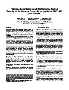
φwd = µX. hAct∆ iX ∨ [Act∆ U ]ff Unlike strong distinguishability, weak distinguishability is not preserved under ioco. This is illustrated by the following example: Example 2. Let F1 and F2 be two fault models and let I be an implementation (see Fig. 1). Clearly, I ioco F1 and I ioco F2 . Moreover, F1 and F2 are weakly distinguishable, as illustrated by the trace ?b.!e. However, I is clearly not weakly distinguishable from itself, as distinguishability is irreflexive. F1 !a

?b

!a !e

I

F2

!a

!a

?b

!e

?b

!a

?b !a

!e

!a

?b Fig. 1. Fault models F1 and F2 and implementation I.

3.2 Orthogonality Whereas distinguishability focuses on the differences in output for two given fault models, it is equally well possible that there is a difference in the specified inputs. Note that this is allowed in ioco-testing theory: a specification does not have to be input complete; this partiality with respect to inputs supports a useful form of underspecification. In practice, a fault hypothesis can often be tested by focusing testing effort on particular aspects. Exploiting the differences in underspecifications of the fault models gives rise to a second heuristic, called orthogonality, which we describe in this section. We start by extending the intersection operator of Def. 4. Definition 7. Let Fi = hSi , ActI , ActU , →i , si i, for i = 1, 2 be two fault models. Assume Θ = {Θa | a ∈ ActI } is a set of fresh constants disjoint from Act∆ . We denote Act ∪ Θ by Act∆ Θ . The orthogonality-aware intersection of F1 and F2 , denoted ∆ F1 ||Θ F2 , is an LTS defined by h(2S1 \ ∅) × (2S2 \ ∅), ActΘ I , ActU , →, ([s1 ]ǫ , [s2 ]ǫ )i, where → is defined by the two rules of Def. 4 in addition to the following two rules: ∅ 6= q1 ⊆ S1

∅ 6= q2 ⊆ S2

[q1 ]a Θa

6= ∅ [q2 ]a = ∅ a ∈ ActI

[q2 ]a Θa

6= ∅ [q1 ]a = ∅ a ∈ ActI

(q1 , q2 ) −−→ (q1 , q2 ) ∅ 6= q1 ⊆ S1

∅ 6= q2 ⊆ S2

(q1 , q2 ) −−→ (q1 , q2 ) 9

Property 4. Let F1 ||Θ F2 be the orthogonality-aware intersection of F1 and F2 , and let (q1 , q2 ) be a state of F1 ||Θ F2 . Then: 1. F1 ||Θ F2 is deterministic, Θa a 2. For all inputs a ∈ ActI , (q1 , q2 ) − → implies (q1 , q2 ) 6−−→. Note that the reverse of Property 4, item 2 does not hold exactly because of the input incompleteness of fault models in general. Intuitively, the occurrence of a label Θa in the orthogonality-aware intersection models the fact that input a is specified by only one of the two LTSs and is left unspecified by the other LTS. The presence of such labels in the orthogonality-aware intersection are therefore pointers to the orthogonality of two systems. Once an experiment arrives in a state with an orthogonality label Θa , testing can focus on one of the two fault models exclusively. Any test failure that is subsequently found is due to the incorrectness of the selected fault model. We next formalise the notions of strong and weak orthogonality, analogously to distinguishability. ∆ Definition 8. Let F1 ||Θ F2 = hS, ActΘ I , ActU , →, si. F1 and F2 are said to be strongly orthogonal if there is a natural number k such that s ∈ OF1 ||Θ F2 (k), where OF1 ||Θ F2 : N → 2S is inductively defined by:  Θa  = {t  OF1 ||Θ F2 (0) T ∈ S | ∃a ∈ ActI : t −−→} OF1 ||Θ F2 (n + 1) = a∈Act∆ {t | [t]a ⊆ OF1 ||Θ F2 (n) ∧ ∃a′ ∈ ActU : [t]a′ 6= ∅}  S U  Θa 6 [t]a ⊆ OF1 ||Θ F2 (n) ∨ t −− −→ } ∪ a∈ActI {t | ∅ =

The following theorem recasts strong orthogonality as a modal property.

Theorem 3. Fault models F1 and F2 are strongly orthogonal iff F1 ||Θ F2 |= φso , where def ∆ φso = µX. (hAct∆ U itt ∧ [ActU ]X) ∨ hActI iX ∨ hΘitt Analogously to distinguishability, we define a weak variation of strong orthogonality, which states that it is possible to reach a state in which an orthogonal label Θa for some a is enabled. ∆ Definition 9. Given F1 ||Θ F2 = hS, ActΘ I , ActU , →, si. F1 and F2 are said to be weakly orthogonal iff der(F1 ||Θ F2 ) ∩ O(0) 6= ∅.

A recast of weak orthogonality into the µ-calculus is as follows. Theorem 4. Fault models F1 and F2 are weakly orthogonal iff F1 ||Θ F2 |= φwo , where def φwo = µX. hAct∆ iX ∨ hΘitt Orthogonality is not preserved under ioco conformance, which is illustrated by the following example. Example 3. Let F1 and F2 be two fault models and let I1 and I2 be two implementations, depicted in Fig. 2. Clearly, I1 ioco F1 and I2 ioco F2 . Moreover, F1 and F2 are (strongly and weakly) orthogonal, as illustrated by the trace ?b.?b which is applicable for F1 , but not applicable for F2 . However, I1 and I2 are not orthogonal. Note that by repeatedly executing experiment ?b.?b and subsequently observing output confidence in the correctness of (aspects of) F1 can increase. 10

F1

F2 !a

?b

!e ?b

?c

?b

I1

?c !a

?b

!e ?b

?c

?c !a

?c

I2 !a

?b ?b

?c

?b, ?c ?b, ?c ?b, ?c Fig. 2. Fault models F1 and F2 and implementations I1 and I2 .

4 Automating Diagnostic Testing In the previous section we formalised the notions of distinguishability and orthogonality, both in terms of set-theory and modal logic. In this section, we rely on the latter results for defining provably correct algorithms for eliminating fault models and for isolating behaviours of fault models for further scrutiny. First, we introduce the basic tools that we rely on for defining our on-the-fly diagnostic testing algorithms and semi-decision procedures. Then, in Section 4.2 we define the algorithms for strong distinguishability and orthogonality, and in Section 4.3, the semi-decision procedures for weak distinguishability and orthogonality are given. 4.1 Preliminaries For the remainder of these sections, we assume that I is an implementation that we wish to subject to diagnostic testing, and Fi = hSi , ActI , ActU , →i , si i, for i = 1, 2 are two (Θ) given fault models. F1 ||(Θ) F2 = hS, ActI , Act∆ U , →, si is the (orthogonality-aware) intersection of F1 and F2 . From this time forth, we assume to have the following four methods at our disposal: 1. Apply(a): send input action a ∈ ActI to an implementation, 2. Observe(): observe some output a ∈ ActU ∪ {δ} from an implementation, 3. Counterexamplea(L, φ): returns an arbitrary counterexample for L |= φ if one exists, and returns ⊥ otherwise. 4. Counterexamples(L, φ): returns one among possibly many shortest counterexamples for L |= φ if a counterexample exists, and returns ⊥ otherwise. We refer to [12] for an explanation of the computation of counterexamples for the modal µ-calculus. In our ordeals we assume that ⊥ is a special character that we can concatenate to sequences of actions. 4.2 Strong Distinguishability and Strong Orthogonality Suppose F1 and F2 are strongly distinguishable or orthogonal. Algorithm 1 derives and executes (on-the-fly) an experiment that (see also Theorem 5), depending on the input: – allows to eliminate at least one fault model from a set of fault models, or 11

– isolates a fault model for further testing. Recall that φ denotes the dual of φ (see Section 2). Informally, the algorithm works as follows for strongly distinguishable fault models F1 and F2 (likewise for strongly orthogonal fault models): η is the shortest counterexample for F1 and F2 not being strongly distinguishable. The algorithm tries to replay η on the implementation, and recomputes a new counterexample when an output produced by the system-under-test does not agree with the output specified in the counterexample. When the counterexample has length 0, we can be sure to have reached a discriminating state, and observing output in this state eliminates at least one of the two considered fault models.

Algorithm 1 Algorithm for exploiting strong distinguishability/orthogonality Require: P ⊆ S, |P | = 1, η is a shortest counterexample for P |= φx , φx ∈ {φsd , φso } Ensure: Returns a sequence executed on I. 1: function A1 (P, η, φx ) 2: if η = ǫ then 3: if φx = φsd then return Observe(); 4: else choose a from {y ∈ ActI | [P ]Θy 6= ∅}; return a; 5: end if 6: else ⊲ Assume η ≡ e η ′ for some action e and sequence η ′ 7: if e ∈ ActI then Apply(e); return e A1 ([P ]e , η ′ , φx ); 8: else a := Observe(); 9: if a = e then return e A1 ([P ]R −1 (e) , η ′ , φx ); 10: else if R−1 (a) ∈ out(P ) then 11: return a A1 ([P ]R −1 (a) , R∗ (Counterexamples([P ]R −1 (a) , φx )), φx ); 12: else return a; 13: end if 14: end if 15: end if 16: end function

Theorem 5. Let F1 and F2 be strongly orthogonal or strongly distinguishable fault models. Let φ = φsd when F1 and F2 are distinguishable and let φ = φso when F1 and F2 are orthogonal. Then algorithm A1 ({s}, Counterexamples(F1 ||Θ F2 , φ), φ) terminates and the sequence σ ≡ σ ′ a it returns satisfies: 1. [F1 ]σ′ 6= ∅ and [F2 ]σ′ 6= ∅ and [I]σ 6= ∅ 2. a ∈ Actδ \ActI implies out([I]σ′ ) 6⊆ out([F1 ]σ′ ) or out([I]σ′ ) 6⊆ out([F2 ]σ′ ), 3. a ∈ ActI implies φ = φso and [F1 ]σ = ∅ or [F2 ]σ = ∅. The sequence that is returned by the algorithm can be used straightforwardly for checking which fault model(s) can be eliminated, or which fault model is selected for further scrutiny (see also Section 4.5). Such “verdicts” are easily added to our algorithms, but are left out for readability. 12

4.3 Weak distinguishability and Weak Orthogonality In case F1 and F2 are not strongly but weakly distinguishable (resp. weakly orthogonal), there is no guarantee that a discriminating (resp. orthogonal) state is reached. By conducting sufficiently many tests, however, chances are that one of such states is eventually reached, unless the experiment has run off to a part of the state space in which no discriminating (resp. orthogonal) states are reachable. Semi-decision procedure 2 conducts experiments on implementation I, and terminates in the following three cases: 1. if a sequence has been executed that led to a discriminating/orthogonal state, 2. if an output was observed that conflicts at least one of the fault models, 3. if discriminating/orthogonal states are no longer reachable. So long as neither of these cases are met, the procedure does not terminate. The semidecision procedure works in roughly the same manner as the algorithm of the previous section. The main differences are in the termination conditions (and the result it returns), and, secondly the use of arbitrary counterexamples, as shorter counterexamples are not necessarily more promising for reaching a discriminating/orthogonal state.

Algorithm 2 Semi-decision procedure for exploiting weak distinguishability/orthogonality Require: P ⊆ S, |P | = 1, η is any counterexample for P |= φx , φx ∈{φwo , φwd } Ensure: Returns a sequence executed on I upon termination 1: function A2 (P, η, φx ) 2: if η = ǫ then 3: if φx = φwd then return Observe(); 4: else choose a from {y ∈ ActI | [P ]Θy 6= ∅}; return a; 5: end if 6: else ⊲ Assume η ≡ e η ′ for some action e and sequence η ′ 7: if e ∈ ActI then Apply(e); return e A2 ([Q]e , η ′ , φx ); 8: else a := Observe(); 9: if a = e then return e A2 ([P ]e , η ′ , φx ); 10: else if R−1 (a)∈out(P ) ∧ Counterexamplea([P ]R −1 (a) , φx ) 6= ⊥ then 11: return a A2 ([P ]R −1 (a) , R∗ (Counterexamplea ([P ]R −1 (a) , φx )), φx ); 12: else if R−1 (a)∈out(P ) ∧ Counterexamplea([P ]R −1 (a) , φx ) = ⊥ then 13: return ⊥; 14: else return a; 15: end if 16: end if 17: end if 18: end function

Theorem 6. Let F1 and F2 be weakly orthogonal or weakly distinguishable fault models. Let φ = φwd when F1 and F2 are distinguishable and let φ = φwo when F1 and F2 are orthogonal. If algorithm A2 ({s}, Counterexamplea(F1 ||Θ F2 , φ), φ) terminates it returns a sequence σ ≡ σ ′ a satisfying: 13

1. 2. 3. 4.

[F1 ]σ′ 6= ∅ and [F2 ]σ′ 6= ∅ and [I]σ 6= ∅ a ∈ Actδ \ActI implies out([I]σ′ ) 6⊆ out([F1 ]σ′ ), or out([I]σ′ ) 6⊆ out([F2 ]σ′ ), a ∈ ActI implies φ = φwo and [F1 ]σ = ∅ or [F2 ]σ = ∅. a = ⊥ implies either φ = φwo and der ([s]σ′ ) ∩ O(0) = ∅, or φ = φso and der([s]σ′ ) ∩ D(0) = ∅.

The following example illustrates that the semi-decision procedure does not necessarily terminate. Example 4. Suppose the intersection of two fault models is given by F1 ||F2 and the malfunctioning implementation is given by I (see Fig. 3). Clearly, F1 and F2 are weakly distinguishable, which means semi-decision procedure 2 is applicable. A counterexample to non-weak distinguishability is e.g. ?b!e?b?b!a, so the procedure might try to execute this sequence. However, termination is not guaranteed, as the implementation may never execute action !a, but output !e instead, making the semi-decision procedure recompute new counterexamples.

∆

F1 kF2

I

?b

?b

?b

?b !a

!a

!e

!e ?b ∆

Fig. 3. No termination guaranteed for semi-decision procedure 2.

4.4 Optimisations The algorithms for strong distinguishability (resp. strong orthogonality) in the previous section can be further optimised in a number of ways. First, one can include a minor addition to the standard model-checking algorithm, marking each k-discriminating (resp. k-orthogonal) state in the LTS that is checked with its depth k. While this has a negligible negative impact on the time complexity of the model checking algorithm, the state markings allow for replacing the method Counterexamples() with a constanttime operation. Secondly, upon reaching a node in D(k) (O(k), respectively), the semidecision procedure for weak distinguishability/orthogonality could continue to behave as algorithm 1. Furthermore, the orthogonality aware intersection is an extension of the plain intersection. Computing both is therefore unnecessary: only the former is needed; in that case, the formulae for strong and weak distinguishability need to be altered to take the extended set of input actions into account. 14

4.5 Diagnostic Testing Methodology Distinguishability and orthogonality, and their associated algorithms, help in reducing the effort that is required for diagnostic testing. Thus far, we presented these techniques without addressing the issue of when a particular technique is worth investigating. In this section, we discuss a methodology for employing these techniques in diagnostic testing. For the remainder of this section, we assume a faulty implementation I and a given set of fault models F = {F1 , . . . , Fn }. We propose a stepwise refinement of the diagnostic testing problem using distinguishability and orthogonality. The first step in our methodology is to identify the largest non-symmetric set of pairs of strongly distinguishable fault models G. We next employ the following strategy: so long as G 6= ∅, select a pair (Fi , Fj ) ∈ G and provide this pair as input to algorithm 1. Upon termination of the algorithm, an experiment σ ≡ σ ′ a is returned, eliminating Fk from F iff a ∈ / out([Fk ]σ′ ) (k = i, j). Moreover, / out([Fl ]σ′ ) and recompute G. remove all fault models Fl for which [Fl ]σ′ 6= ∅ and a ∈ A worst case scenario requires at most |G| iterations to reach G = ∅. The process can be further optimised by ordering fault models w.r.t. ioco-testing power, but it is beyond the scope of this paper to elaborate on this. When G is empty, no strongly distinguishable pair can be found in F . The set of fault models can be further reduced using the weak distinguishability and strong orthogonality heuristics, in no particular order, as neither allows for a fail-safe strategy to a conclusive verdict. As a last resort, weak orthogonality is used before conducting naive testing using the remaining fault models.

5 Example As an illustration of some of the techniques that we presented in this paper, we consider a toy example concerning the prototypical coffee machine. The black-box behaviour of the coffee-machine is defined by specification S in Fig. 4, where action ?c and !c represent a coffee request and production, ?t and !t represent a tea request and production, and ?m and !m represent a coffee-cream request and production. Among the set of fault F1

S !c ?t ?c !m

F1 ||F2

F2 ?c, ?t

?c, ?t, ?m !t ?m

!∆ !c, !t

?c, ?t

F1 ||Θ F2 !∆, ?Θm ?c, ?t ?Θc , ?Θt , ?Θm

Fig. 4. Specification S and fault models F1 , F2 and F3 of a coffee machine

models for a misbehaving implementation of S are fault models F1 (modelling e.g. a broken keypad in the machine) and F2 (modelling e.g. a broken recipe book). Computing their intersection and their orthogonal-aware intersection, we find that F1 and F2 are strongly distinguishing and strongly orthogonal. The preferred choice here would be to run algorithm 1 with arguments setting it to check for strong distinguishability using e.g. ?t as input for the shortest counterexample. Algorithm 1 would first offer 15

?t to the implementation (which is accepted by assumption that implementations are input-enabled). Since then the shortest counterexample to non-strong distinguishability would be the empty string ǫ, the algorithm queries the output of the implementation and terminates. Any output the implementation produces either violates F1 or F2 , or both. In case one would insist on using strong orthogonality, algorithm 1 would be used with the emtpy string ǫ as the shortest counterexample to non-strong orthogonality. The algorithm would return the sequence ?m, indicating that isolated aspects of F1 can be tested by experiments starting with input ?m.

6 Concluding Remarks We considered the problem of diagnosis for reactive systems, the problem of finding an explanation for a detected malfunction of a system. As an input to the diagnosis problem, we assumed a set of fault models. Each fault model provides a formal explanation of the behaviour of an implementation in terms of an LTS model. From this set of fault models, those models that do not correctly describe (aspects of) the implementation must be eliminated. As may be clear, this can be done naively by testing the implementation against each fault model separately, but this is quite costly. We have introduced several methods, based on model-based testing and model checking techniques, to make this selection process more effective. Concerning issues for future research, we feel that the techniques that we have described in this paper can be further improved upon by casting our techniques in a quantitative framework. By quantifying the differences and overlap between the outputs described by two fault models, a more effective strategy may be found. The resulting quantitative approach can be seen as a generalisation of our notion of weak distinguishability. Such a quantitative approach may very likely employ techniques developed in model checking with costs (or rewards). A second issue that we intend to investigate is the transfer of our results to the setting of real-time, in particular for fault models given by Timed Automata. In our discussions, we restricted our attention to the problem of selecting the right fault models from a set of explicit fault models by assuming this set was obtained manually, thereby side-stepping the problem of obtaining such fault models in the first place. Clearly, identifying techniques for automating this process is required for a full treatment of diagnosis for LTSs. Lastly, and most importantly, the efficacy of the techniques that we have developed in this paper must be assessed on real-life case-studies. There is already some compelling evidence of their effectiveness in [7] where a notion of distinguishability is successfully exploited in the setting of communicating FSM nets. Acknowledgement The authors would like to thank Vlad Rusu, Jan Tretmans and Ren´e de Vries for stimulating discussions and advice on the subjects of diagnosis and testing.

References 1. R. Alur, C. Courcoubetis, and M. Yannakakis. Distinguishing tests for nondeterministic and probabilistic machines. In STOC ’95: Proceedings of the twenty-seventh annual ACM symposium on Theory of computing, pages 363–372, New York, NY, USA, 1995. ACM Press.

16

2. A. Belinfante, J. Feenstra, R.G. de Vries, J. Tretmans, N. Goga, L. Feijs, S. Mauw, and L. Heerink. Formal test automation: A simple experiment. In G. Csopaki, S. Dibuz, and K. Tarnay, editors, Testcom ’99, pages 179–196. Kluwer, 1999. 3. J.C. Bradfield and C.P. Stirling. Modal logics and mu-calculi: an introduction. In J. Bergstra, A. Ponse, and S. Smolka, editors, Handbook of Process Algebra, chapter 4, pages 293–330. Elsevier, 2001. 4. K. El-Fakih, S. Prokopenko, N. Yevtushenko, and G. von Bochmann. Fault diagnosis in extended finite state machines. In D. Hogrefe and A. Wiles, editors, Proc. TestCom 2003, volume 2644 of LNCS, pages 197–210. Springer-Verlag, 2003. 5. K. El-Fakih, N. Yevtushenko, and G. von Bochmann. Diagnosing multiple faults in communicating finite state machines. In Proc. FORTE’01, pages 85–100. Kluwer, B.V., 2001. 6. J.C. Fernandez, C. Jard, T. J´eron, and G. Viho. Using on-the-fly verification techniques for the generation of test suites. In R. Alur and T.A. Henzinger, editors, Proceedings of CAV’96, volume 1102 of LNCS, pages 348–359. Springer-Verlag, 1996. 7. M. Gromov, A. Kolomeetz, and N. Yevtushenko. Synthesis of diagnostic tests for fsm nets. Vestnik of TSU, 9(1):204–209, 2004. 8. M. Gromov and T.A.C. Willemse. Testing and model-checking techniques for diagnosis. In A. Petrenko et al, editor, Proc. TestCom/Fates 2007, volume 4581 of LNCS, pages 138–154. Springer-Verlag, 2007. 9. Q. Guo, R.M. Hierons, M. Harman, and K. Derderian. Heuristics for fault diagnosis when testing from finite state machines. Softw. Test. Verif. Reliab., 17:41–57, 2007. 10. C. Jard and T. J´eron. Tgv: theory, principles and algorithms. STTT, 7(4):297–315, 2005. 11. T. J´eron, H. Marchhand, S. Pinchinat, and M.-O. Cordier. Supervision patterns in discrete event systems diagnosis. In Proc. WODES 2006. IEEE, 2006. 12. A. Kick. Generation of Counterexamples and Witnesses for Model Checking. PhD thesis, Fakult¨at f¨ur Informatik, Universit¨at Karlsruhe, Germany, July 1996. 13. G. Lamperti, M. Zanella, and P. Pogliano. Diagnosis of active systems by automata-based reasoning techniques. Applied Intelligence, 12(3):217–237, 2000. 14. A. Petrenko and N. Yevtushenko. On test derivation from partial specifications. In FORTE/PSTV 2000: Proceedings of the FIP TC6 WG6.1 Joint International Conference on Formal Description Techniques for Distributed Systems and Communication Protocols (FORTE XIII) and Protocol Specification, Testing and Verification (PSTV XX), pages 85– 102, Deventer, The Netherlands, The Netherlands, 2000. Kluwer, B.V. 15. A. Petrenko and N. Yevtushenko. Testing from partial deterministic fsm specifications. IEEE Trans. Comput., 54(9):1154–1165, 2005. 16. J. Pietersma, A.J.C. van Gemund, and A. Bos. A model-based approach to sequential fault diagnosis. In Proceedings IEEE AUTOTESTCON 2005, 2005. 17. J. Tretmans. Test generation with inputs, outputs and repetitive quiescence. Software— Concepts and Tools, 17(3):103–120, 1996.

17

7 Appendix In this section we give proofs for properties and theorems proposed in the main part of the paper. In some of the theorems (namely theorems 1, 2, 3 and 4), we rely on the well-known technique [3] of so called approximation. Definition 10. Approximant terms are defined by induction as follows: ( def µ0 X.ϕ(X) = ff def

µk+1 X.ϕ(X) = ϕ(µk X.ϕ(X))

Approximant terms have following property [3]: µX.ϕ(X) = semantically: [µX.ϕ(X)]]F η

W|S|

k=0

µk X.ϕ(X), or

|S| [ = [µk X.ϕ(X)]]F η,

(MI)

0

where S is set of states of a given LTS L. 7.1 Proofs for section 3 Property 1. Let F1 ||F2 be the intersection of F1 and F2 , and let s1 be a state of F1 , s2 be a state of F2 , (q1 , q2 ) be a state of F1 ||F2 and σ ∈ Act∗δ . Then: 1. F1 ||F2 is deterministic, 2. [([s1 ]σ , [s2 ]σ )]a 6= ∅ implies ([s1 ]σR(a) , [s2 ]σR(a) ) ∈ [([s1 ]σ , [s2 ]σ )]a , 3. out(([q1 ]ǫ , [q2 ]ǫ )) \ {δ} = R−1 (out([q1 ]ǫ ) ∩ out([q2 ]ǫ )). Proof. Let F1 ||F2 be as stated. We prove each property separately. ∗

1. Ad determinacy of F1 ||F2 . Let (q1 , q2 ) be a state of F1 ||F2 , and let σ ∈ Act∆ . We use induction on the length of σ to show that |[(q1 , q2 )]σ | ≤ 1. (a) Case |σ| = 0. This means σ = ǫ. Since F1 ||F2 does not have τ -transitions, [(q1 , q2 )]ǫ = {(q1 , q2 )}. Hence, |[(q1 , q2 )]ǫ | = 1. (b) Case |σ| = n + 1. As our Induction Hypothesis, we take n

∀ρ ∈ Act∆ : |[(q1 , q2 )]ρ | ≤ 1 n

(IH)

Let a ∈ Act∆ and ρ ∈ Act∆ , such that σ ≡ ρa. Then [(q1 , q2 )]ρa = [[(q1 , q2 )]ρ ]a . By our induction hypothesis, we obtain that |[(q1 , q2 )]ρ | ≤ 1. We distinguish two cases: i. Case |[(q1 , q2 )]ρ | = 0. This means [(q1 , q2 )]ρ = ∅, in which case |[[(q1 , q2 )]ρ ]a | = |[∅]a | = 0 18

ii. Case |[(q1 , q2 )]ρ | = 1. This means that for some q1′ , q2′ , [(q1 , q2 )]ρ = {(q1′ , q2′ )}, in which case |[[(q1 , q2 )]ρ ]a | = |[{(q1′ , q2′ )}]a | Since F1 ||F2 contains no τ transitions, and since [ ] is a functional relation on the set of states of F1 and F2 , we obtain  1 if [q1′ ]R(a) 6= ∅ and [q2′ ]R(a) 6= ∅ |[{(q1′ , q2′ )}]a | = 0 otherwise ∗

Hence, we conclude that for all σ ∈ Act∆ , |[(q1 , q2 )]σ | ≤ 1, which proves that F1 ||F2 is deterministic. 2. Ad [([s1 ]σ , [s2 ]σ )]a = {([s1 ]σR(a) , [s2 ]σR(a) )} or [([s1 ]σ , [s2 ]σ )]a = ∅. Follows immediately from Def. 4 and the fact that F1 ||F2 is deterministic 3. Ad out(([q1 ]ǫ , [q2 ]ǫ )) \ {δ} = R−1 (out([q1 ]ǫ ) ∩ out([q2 ]ǫ )). Suppose a ∈ out(([q1 ]ǫ , [q2 ]ǫ )) \ {δ} This is equivalent to a ∈ Act∆ U ∧ [([q1 ]ǫ , [q2 ]ǫ )]a 6= ∅ which, according to Def. 4 holds iff a ∈ Act∆ U ∧ [q1 ]R(a) 6= ∅ ∧ [q2 ]R(a) 6= ∅. This is equivalent to a ∈ Act∆ U ∧ R(a) ∈ out([q1 ]ǫ ) ∩ out([q2 ]ǫ ) which is equivalent to a ∈ R−1 (out([q1 ]ǫ ) ∩ out([q2 ]ǫ )) ⊓ ⊔ To prove property 3 we first repeat the definition of ioco and immediately generalise it to a relation on sets of states. Definition 11. Let Fi = hSi , ActI , ActU , →i , si i (for i = 1, 2) be two LTSes. Let s1 ∈ S1 and s2 ∈ S2 . Then s1 is ioco-conforming to s2 , denoted s1 ioco s2 , when s1 is input-enabled and ∀σ ∈ s-traces(s2 ) : out([s1 ]σ ) ⊆ out([s2 ]σ ) We generalise the ioco-conformance relation to sets of states as follows: q1 ⊆ S1 is ioco-conformant w.r.t. q2 ⊆ S2 , denoted q1 ioco q2 , iff all states s1 ∈ q1 are inputenabled and ∀σ ∈ s-traces(q2 ) : out([q1 ]σ ) ⊆ out([q2 ]σ ), S where s-traces(q2 ) = s1 ∈q1 s-traces(s1 ). The LTSes L1 and L2 are ioco-conforming if s1 ioco s2 . Theorem 7. Let Fi (for i = 1, . . . , 4) be LTSes with sets of states Si . Then for all k ∈ N, and all subsets q1 ⊆ S1 , q2 ⊆ S2 , p1 ⊆ S3 and p2 ⊆ S4 , we have: [p1 ]ǫ ioco [q1 ]ǫ ∧ [p2 ]ǫ ioco [q2 ]ǫ ∧ ([q1 ]ǫ , [q2 ]ǫ ) ∈ D(k) ⇒ ([p1 ]ǫ , [p2 ]ǫ ) ∈ D(k) 19

Proof. Let Fi (for i = 1, . . . , 4) be LTSes with sets of states Si . We denote the set of states of Fi ||Fj by SFi ||Fj (for i, j = 1, . . . , 4). Let q1 ⊆ S1 , q2 ⊆ S2 , p1 ⊆ S3 and p2 ⊆ S4 . Assume that [p1 ]ǫ ioco [q1 ]ǫ and [p2 ]ǫ ioco [q2 ]ǫ . We proceed by using induction on k. 1. Case k = 0. Assume ([q1 ]ǫ , [q2 ]ǫ ) ∈ D(0), i.e. out(([q1 ]ǫ , [q2 ]ǫ )) = {δ}. According to Property 1, we find: R−1 (out([q1 ]ǫ ) ∩ out([q2 ]ǫ )) = ∅ (= out([q1 ]ǫ ) ∩ out([q2 ]ǫ ))

(*)

Since [pi ]ǫ ioco qi (for i = 1, 2) we have: out([pi ]ǫ ) ⊆ out([qi ]ǫ ) for i = 1, 2

(**)

Combining (*) with (**) yields out([p1 ]ǫ ) ∩ out([p2 ]ǫ ) = ∅. Since out never renders the empty set, we can apply Property 1 once again and obtain out(([p1 ]ǫ , [p2 ]ǫ )) = {δ} from which we conclude that ([p1 ]ǫ , [p2 ]ǫ ) ∈ D(0). 2. Case k = n + 1. As our induction hypothesis, we take: ∀q1′ ⊆ S1 , q2′ ⊆ S2 , p′1 ⊆ S3 , p′2 ⊆ S4 : [p′1 ]ǫ ioco [q1′ ]ǫ ∧ [p′2 ]ǫ ioco [q2′ ]ǫ ∧ ([q1′ ]ǫ , [q2′ ]ǫ ) ∈ D(n) ⇒ ([p′1 ]ǫ , [p′2 ]ǫ ) ∈ D(n)

(IH)

Assume ([q1 ]ǫ , [q2 ]ǫ ) ∈ D(n T + 1). We distinguish two cases: (a) Case ([q1 ]ǫ , [q2 ]ǫ ) ∈ a∈Act∆ {(r1 , r2 ) ∈ SF1 ||F2 | [(r1 , r2 )]a ⊆ D(n)}. Let U a ∈ Act∆ U be an arbitrary output action. Then [([q1 ]ǫ , [q2 ]ǫ )]a ⊆ D(n). Using Property 1, this is equivalent to ([q1 ]R(a) , [q2 ]R(a) ) ∈ D(n) or [([q1 ]ǫ , [q2 ]ǫ )]a = ∅ Remark that when [([q1 ]ǫ , [q2 ]ǫ )]a = ∅, we have [qi ]R(a) = ∅ for either i = 1 or i = 2. Because we have [pi ]ǫ ioco [qi ]ǫ we necessarily have [([p1 ]ǫ , [p2 ]ǫ )]a = ∅, from which we immediately obtain ([p1 ]ǫ , [p2 ]ǫ ) ∈ {(r1 , r2 ) ∈ SF3 ||F4 | [(r1 , r2 )]a ⊆ D(n)} Without loss of generality, we therefore assume that ([q1 ]R(a) , [q2 ]R(a) ) ∈ D(n) and [([p1 ]ǫ , [p2 ]ǫ )]a 6= ∅. This means that R(a) ∈ out([p1 ]ǫ )∩out([p2 ]ǫ ) ⊆ out([q1 ]ǫ ) ∩ out([q2 ]ǫ ). Under the assumption that we have, for i = 1, 2, [pi ]ǫ ioco [qi ]ǫ we conclude that [pi ]R(a) ioco [qi ]R(a) . By taking qi′ = [qi ]R(a) , and p′i = [pi ]R(a) , we can apply the induction hypothesis and obtain: ([p1 ]R(a) , [p2 ]R(a) ) ∈ D(n) Using Property 1 once again, this is equivalent to [([p1 ]ǫ , [p2 ]ǫ )]a ⊆ D(n). Therefore, we conclude that: ([p1 ]ǫ , [p2 ]ǫ ) ∈ {(r1 , r2 ) ∈ SF3 ||F4 | [(r1 , r2 )]a ⊆ D(n)} Hence, we have for all a ∈ Act∆ U : [([p1 ]ǫ , [p2 ]ǫ )]a ⊆ D(n). Therefore: \ {(r1 , r2 ) ∈ SF3 ||F4 | [(r1 , r2 )]a ⊆ D(n)} ([p1 ]ǫ , [p2 ]ǫ ) ∈ a∈Act∆ U

20

S (b) Case ([q1 ]ǫ , [q2 ]ǫ ) ∈ a∈ActI {(r1 , r2 ) ∈ SF1 ||F2 | ∅ = 6 [(r1 , r2 )]a ⊆ D(n)}. Pick an input a ∈ ActI , such that ∅ 6= [([q1 ]ǫ , [q2 ]ǫ )]a ⊆ D(n) Using Property 1, we therefore obtain ([q1 ]R(a) , [q2 ]R(a) ) ∈ D(n). Since a ∈ ActI , we have R(a) = a. Under our assumption that, for i = 1, 2, [pi ]ǫ ioco [qi ]ǫ we conclude both: i. [pi ]a ioco [qi ]a , and, ii. [pi ]a 6= ∅. Applying the induction hypothesis, taking qi′ = [qi ]a and p′i = [pi ]a , we obtain: ([p1 ]a , [p2 ]a ) ∈ D(n) Using Property 1 this is equivalent to [([p1 ]ǫ , [p2 ]ǫ )]a ⊆ D(n). In combination with ii), this leads to: 6 [(r1 , r2 )]a ⊆ D(n)} ([p1 ]ǫ , [p2 ]ǫ ) ∈ {(r1 , r2 ) ∈ 2S3 × 2S4 | ∅ = Therefore: ([p1 ]ǫ , [p2 ]ǫ ) ∈

[

6 [(r1 , r2 )]a ⊆ D(n)} {(r1 , r2 ) ∈ 2S3 × 2S4 | ∅ =

a∈ActI

Both cases lead to the conclusion ([p1 ]ǫ , [p2 ]ǫ ) ∈ D(n + 1) = D(k), which finishes the proof. ⊓ ⊔ Now property 3 becomes just a corollary of theorem 7: Property 3. Let F1 , F2 be fault models, and let I1 , I2 be implementations. If I1 ioco F1 and I2 ioco F2 and F1 and F2 are strongly distinguishable, then so are I1 and I2 . Proof. Let sF1 be the initial state of LTS F1 , sF2 – F2 , sI1 – I1 , sI2 – I2 . By definition, fact, that I1 ioco F1 and I2 ioco F2 , means that sI1 ioco sF1 and sI2 ioco sF2 hold, and from this, we conclude that [sI1 ]ǫ ioco [sF1 ]ǫ and [sI2 ]ǫ ioco [sF2 ]ǫ hold. Assume F1 and F2 are distinguishable. Then, for some k ∈ N, we have ([sF1 ]ǫ , [sF2 ]ǫ ) ∈ D(k). Applying Lemma 7, we find ([sI1 ]ǫ , [sI2 ]ǫ ) ∈ D(k). Therefore, I1 and I2 are distinguishable. ⊓ ⊔

Theorem 1. Let F1 , F2 be two fault models. Then F1 and F2 are strongly distinguishable iff F1 ||F2 |= φsd , where def

φsd = µX. [Act∆ U ]X ∨ hActI iX W V Proof. We abbreviate a∈Act∆ [a]X∨ a∈ActI haiX by ϕ(X) and we abbreviate F1 ||F2 U W V by L (recall, that [A]φ is a shorthand for a∈A [a] φ and hAiφ for a∈A haiφ). First, we prove, by induction, that ∀k ∈ N D(k) = [µk+1 X.ϕ(X)]]L η where η : X → 2S is a propositional environment and S is the state space of L. For brevity, from hereon, we omit the indices L and η. Recall that we have [µ0 X.ϕ(X)]] = [ff]] = ∅. 21

1. Base case: [µ1 X.ϕ(X)]] = [ϕ(X)]][∅/X] = ^ _ =[ [a]X]][∅/X] ∪ [ haiX]][∅/X] = a∈ActI

a∈Act∆ U

\

=

′

a {q ∈ S | ∀q ∈ S : q −→ q ′ ⇒ q ′ ∈ ∅} ∪

a∈Act∆ U

∪

[

a {q ∈ S| ∃q ′ ∈ S : q −→ q ′ ∧ q ′ ∈ ∅} =

a∈ActI

= {q ∈ S | out([q]ǫ ) = {δ}} ∪ ∅ = D(0) where S is the set of states of L. 2. Inductive step: as our induction hypothesis, we state: [µk+1 X.ϕ(X)]] = D(k)

(IH)

We reason as follows: [µk+2 X.ϕ(X)]] = =∗ = = ∪

[ϕ(X)]][ [µk+1 X.ϕ(X)]]/X ] [V ϕ(X)]]D(k)/X ] W [ a∈Act∆ [a]X]][D(k)/X] ∪ [ a∈ActI haiX]][D(k)/X] U T a ′ ′ ′ ∆ {q ∈ S | ∀q ∈ S : q −→ q ⇒ q ∈ D(k)} Sa∈ActU a ′ ′ ′ a∈ActI {q ∈ S | ∃q ∈ S : q −→ q ∧ q ∈ D(k)}

where, at ∗, we used the induction hypothesis. Since LTS L is deterministic (Property 1) and according to definition of [ ] -operator we have: a (q −→ q ′ ) ⇔ (q ′ ∈ [q]a )

Therefore: a ∀q ′ ∈ S : q −→ q ′ ⇒ q ′ ∈ D(k) ′ ′ ⇔ ∀q ∈ [q]a : q ∈ D(k) ⇔ [q]a ⊆ D(k)

Similarly, we simplify: a ∃q ′ ∈ S : q −→ q ′ ∧ q ′ ∈ D(k) ′ ⇔ [q]a 6= ∅ ∧ {q } = [q]a ∧ q ′ ∈ D(k) ⇔∅= 6 [q]a ⊆ D(k)

So, T [µk+2 X.ϕ(X)]] = a∈Act∆ {q ∈ S | [q]a ⊆ D(k)} U S 6 [q]a ⊆ D(k)} = ∪ a∈ActI {q ∈ S | ∅ = = D(k) 22

Hence, for all k ∈ N, we have: D(k) = [µk+1 X.ϕ(X)]]L η

(†)

We use this to prove the theorem: “⇒” Now, if the initial state q0 of F1 ||F2 is such, that q0 ∈ D(k) for some k, (i.e., F1 and F2 are strongly distinguishable), then, because of † and (MI), q0 ∈ [µX.ϕ(X)]]L η, which means that F1 ||F2  φsd . “⇐” If F1 ||F2  φsd , then, by semantics of the µ-calculus, we have q0 ∈ [µX.ϕ(X)]]L η, whereSq0 is the initial state of F1 ||F2 . From the correspondence (MI), we obtain q0 ∈ 0≤i≤|S|[µi X.ϕ(X)]]L η which implies that there is a 0 < k ≤ |S|, such that q0 ∈ [µk X.ϕ(X)]]L . From †, we immediately obtain q0 ∈ D(k −1) for some k > 0, η which means that F1 and F2 are strongly distinguishable. ⊓ ⊔

Theorem 2. Let F1 , F2 be two fault models. Then F1 and F2 are weakly distinguishable iff F1 ||F2 |= φwd , where def

φwd = µX. hAct∆ iX ∨ [Act∆ U ]ff Proof. We closelyVfollow the proof strategy of Theorem 1. Let ϕ(X) denote the formula W [a]ff and let L = F1 ||F2 . We prove the following property a∈Act∆ a∈Act haiX ∨ U by induction on k ∈ N: {s ∈ S | ∃σ ∈ (Act∆ )≤k : [s]σ ∩ D(0) 6= ∅} = [µk+1 X.ϕ(X)]] 1. Base case: [µ1 X.ϕ(X)]] = [ϕ(X)] V W ][∅/X] = = [ a∈Act∆ haiX ∨ a∈Act∆ [a]ff]][∅/X] = U S a q ′ ∧ q ′ ∈ ∅} = Ta∈Act∆ {q ∈ S | ∃q ′ ∈ S : q −→ a ′ ∪ a∈Act∆ {q ∈ S | ∀q ∈ S : q −→ q ′ ⇒ q ′ ∈ ∅} U = {q ∈ S | [q]ǫ ∩ D(0) 6= ∅} = {q ∈ S | ∃σ ∈ (Act∆ )≤0 : [q]σ ∩ D(0) 6= ∅} 2. Inductive step: as our induction hypothesis, we state: {s ∈ S | ∃σ ∈ (Act∆ )≤k : [s]σ ∩ D(0) 6= ∅} = [µk+1 X.ϕ(X)]] For short, we define the function Σ : N → 2S as follows: Σ(k) = {s ∈ S | ∃σ ∈ (Act∆ )≤k : [s]σ ∩ D(0) 6= ∅} 23

(IH)

We proceed as follows: [µk+2 X.ϕ(X)]] = [ϕ(X)]][ [µk+1 X.ϕ(X)]]/X ] =∗ [S ϕ(X)]][ Σ(k)/X ] a = Ta∈Act∆ {q ∈ S | ∃q ′ ∈ S : q −→ q ′ ∧ q ′ ∈ Σ(k)} a ′ ′ ′ ∪ ∆ {q ∈ S | ∀q ∈ S : q −→ q ⇒ q ∈ ∅} Sa∈ActU ∆ ≤k : [q]aσ ∩ D(0) 6= ∅} = a∈Act∆ {q ∈ S | ∃σ ∈ (Act ) ∪ {q ∈ S | [q]ǫ ∩ D(0) 6= ∅} = {q ∈ S | ∃ρ ∈ (Act∆ )≤k+1 : [q]ρ ∩ D(0) 6= ∅} Hence, for all k ∈ N, we have: {s ∈ S | ∃σ ∈ (Act∆ )≤k : [s]σ ∩ D(0) 6= ∅} = [µk+1 X.ϕ(X)]]

(‡)

We continue proving theorem 2. “⇒” Suppose F1 and F2 are weakly distinguishable, i.e. der(q0 ) ∩ D(0) 6= ∅. This means that q0 ∈ {s ∈ S | ∃σ ∈ (Act∆ )≤k : [s]σ ∩ D(0) 6= ∅}. From ‡, we immediately have q0 ∈ [µk+1 X.ϕ(X)]], and, using (MI), we find q0 ∈ [µX.ϕ(X)]], i.e. F1 ||F2 |= φwd . “⇐” Suppose that F1 ||F2 |= φwd . This means that q0 ∈ [µX.ϕ(X)]], and, using (MI), there is some 0 < i ≤ |S|, such that q0 ∈ [µX i .ϕ(X)]]. By ‡, we find that der(q0 )∩ D(0) 6= ∅. ⊓ ⊔

Property 4. Let F1 ||Θ F2 be the orthogonality-aware intersection of F1 and F2 , and let (q1 , q2 ) be a state of F1 ||Θ F2 . Then: 1. F1 ||Θ F2 is deterministic, Θ

a

a 2. For all inputs a ∈ ActI , (q1 , q2 ) − → implies (q1 , q2 ) − 6 −→.

Proof. Let F1 ||Θ F2 be as stated. 1. The proof of determinacy of F1 ||Θ F2 closely follows the proof of Property 1. a 2. Let (q1 , q2 ) be a state in F1 ||Θ F2 . Assume (q1 , q2 ) − → for some a ∈ ActI . Then Θ

a [q1 ]a 6= ∅ and [q2 ]a 6= ∅. Therefore, (q1 , q2 ) − 6 −→.

⊓ ⊔

∆ Theorem 3. Given F1 ||Θ F2 = hS, ActΘ I , ActU , →, si.Then F1 and F2 are strongly orthogonal iff F1 ||Θ F2 |= φso , where def

∆ φso = µX. (hAct∆ U itt ∧ [ActU ]X) ∨ hActI iX ∨ hΘitt

24

W V W W Proof. We abbreviate ( a∈Act∆ haitt∧ a∈Act∆ [a]X)∨ a∈ActI haiX∨ a∈ActI hΘa itt U U by φ(X). L abbreviates F1 ||Θ F2 and has state space S; we omit indices in the interpretation of µ-calculus formulae. We establish the following correspondence by means of an inductive proof: ∀k ∈ N : [µk+1 X.ϕ(X)]] = O(k) 1. Base case: [µ1 X.ϕ(X)]] = [ϕ(X)] W ][∅/X] = V = [ a∈Act∆ haitt ∧ a∈Act∆ [a]X]][∅/X] U WU W ∪ [ Sa∈ActI haiX]][∅/X] ∪ [ a∈ActI hΘa itt]][∅/X] a q ′ ∧ q ′ ∈ S}∩ = ( a∈Act∆ {q ∈ S | ∃q ′ ∈ S : q −→ U T a ′ ′ ′ ∆ {q ∈ S | ∀q ∈ S : q −→ q ⇒ q ∈ ∅}) S a∈ActU a ′ ′ ′ ∪ a∈ActI {q ∈ S | ∃q ∈ S : q −→ q ∧ q ∈ ∅} S Θa −→ q ′ ∧ q ′ ∈ S} ∪ a∈ActI {q ∈ S | ∃q ′ ∈ S : q −− a a ∆ = ({q ∈ S | ∃a ∈ ActU : q −→ } ∩ {q ∈ S | ∀a ∈ Act∆ / }) U : q −−→ Θa ∪ {q ∈ S | ∃a ∈ ActI : q −− −→ } Θa = {q ∈ S | ∃a ∈ ActI : q −− −→ } = O(0) 2. Inductive step: as our induction hypothesis, we take: [µk+1 X.ϕ(X)]] = O(k)

(IH)

We continue: [µk+2 X.ϕ(X)]] = [ϕ(X)]][ [µk+1 X.ϕ(X)]]/X ] =(IH) [ϕ(X)] W ][O(k)/X] =V = [ a∈Act∆ haitt ∧ a∈Act∆ [a]X]][O(k)/X] UW U W ∪ [ Sa∈ActI haiX]][O(k)/X] ∪ [ a∈ActI hΘa itt]][O(k)/X] a = ( a∈Act∆ {q ∈ S | ∃q ′ ∈ S : q −→ q ′ ∧ q ′ ∈ S}∩ U T a ′ ′ ′ ∆ {q ∈ S | ∀q ∈ S : q −→ q ⇒ q ∈ O(k)}) S a∈ActU a ′ ′ ′ {q ∈ S | ∃q ∈ S : q −→ q ∧ q ∈ O(k)} ∪ Sa∈ActI Θa ′ ∪ − −→ q ′ ∧ q ′ ∈ S} a∈ActI {q ∈ S | ∃q ∈ S : q − = O(k + 1) Hence, we find for all k ∈ N: O(k) = [µk+1 X.ϕ(X)]] Using this correspondence, the proof of Theorem 3 continues along the lines of the proof of Theorem 1. ⊓ ⊔

Theorem 4. Fault models F1 and F2 are weakly orthogonal iff F1 ||Θ F2 |= φwo , where def

φwo = µX. hAct∆ iX ∨ hΘitt 25

W W Proof. Let ϕ(X) = a∈Act∆ haiX ∨ a∈ActI hΘa itt. We abbreviate F1 ||Θ F2 by L and denote its state space by S. The following correspondence can be proved inductively, following the line of reasoning that was followed for the inductive proof that was central to the proof of Theorem 2: ∀k ∈ N : {s ∈ S | ∃σ ∈ (Act∆ )≤k : [s]σ ∩ O(0) 6= ∅} = [µk+1 X.ϕ(X)]] ⊓ ⊔ 7.2 Proofs for section 4 Theorem 5. Let F1 and F2 be strongly orthogonal or strongly distinguishable fault models. Let φ = φsd when F1 and F2 are distinguishable and let φ = φso when F1 and F2 are orthogonal. Then algorithm A1 ({s}, Counterexamples(F1 ||Θ F2 , φ), φ) terminates and the sequence σ ≡ σ ′ a it returns satisfies: 1. [F1 ]σ′ 6= ∅ and [F2 ]σ′ 6= ∅ and [I]σ 6= ∅, 2. a ∈ Actδ \ActI implies out([I]σ′ ) 6⊆ out([F1 ]σ′ ) or out([I]σ′ ) 6⊆ out([F2 ]σ′ ), 3. a ∈ ActI implies φ = φso and [F1 ]σ = ∅ or [F2 ]σ = ∅. Proof. Due to the analogous definitions of distinguishability and orthogonality, we focus on a proof for strong distinguishability only. As a result of Theorems 1, we know that the initial state (q1 , q2 ) of F1 ||F2 satisfies (q1 , q2 ) ∈ D(k) for some k ∈ N. We show that the bound k strictly decreases in each recursive call to A1 . In particular, we show by means of an inductive proof that at recursive call i (i ≤ k), the parameter P satisfies P ⊆ D(k − i) and |η| ≤ k − i. 1. Base case (i = 0): since initially P = {s}, where s is the initial state of F1 ||F2 , we have P ⊆ D(k) = D(k − i). 2. Suppose that at recursion call i (i < k), the parameter P satisfies P ⊆ D(k − i) and |η| ≤ k − i. If η = ǫ, then the recursion terminates, so without loss of generality, we assume that η ≡ e η ′ for some action e and trace η ′ . We show that at each next call to A1 , we have P ⊆ D(k − (i + 1)) and |η| ≤ k − (i + 1). We distinguish the following cases: (a) Case e ∈ ActI . Since η is a shortest counterexample for P |= φsd , we know that [P ]e ⊆ D(k − (i + j)) for some j ≥ 1. Because of Property 2, we know that D(k − (i + j)) ⊆ D(k − (i + 1)), and therefore [P ]e ⊆ D(k − (i + 1)). Clearly, |η ′ | = |η| − 1, and, by induction, |η ′ | ≤ k − (i + 1). (b) Case e ∈ / ActI . This means that the algorithm observes output a from the implementation. Depending on a, we distinguish two cases: i. Case R−1 (a) ∈ out(P ). Since P ⊆ D(k − i), and a is an output, we have, by definition of D( ) that [P ]R(a) ⊆ D(k − (i + 1)). The new counterexample that is generated is therefore at most of length k − (i + 1), so at recursive call i + 1, we have |η| ≤ k − (i + 1). ii. Case R−1 (a) ∈ / out(P ). The recursion terminates immediately. Concluding, we find that the algorithm terminates within k steps. 26

Next, we prove the remainder of our proof obligations. 1. The property [F1 ]σ′ 6= ∅, and [F2 ]σ′ 6= ∅ both follow from the observation that [F1 ||F2 ]R−1∗ (σ′ ) 6= ∅ and property 1, and the fact that η is always a counterexample of φsd for F1 ||F2 . The property [I]σ 6= ∅ follows from the fact that the implementation is input-enabled and that each output in σ comes from I, which is easily checked. 2. Suppose a ∈ Actδ \ ActI . Since a is the final action, this means that a can only have been obtained in the following cases: (a) η = ǫ, which means that [(F1 ||F2 )]R∗ (σ′ ) ⊆ D(0), i.e. the trace σ ′ led to a discriminating state. This implies that out([(F1 ||F2 )]R∗ (σ′ ) ) = {δ}, which in turn implies that out([F1 ]σ′ ) ∩ out([F2 ]σ′ ) = ∅. Since [I]σ′ 6= ∅, we find out([I]σ′ ) 6⊆ out([Fi ]σ′ ) for at least one i ∈ {1, 2}. (b) η 6= ǫ, which means that a is such that R−1 (a) 6∈ out(P ). Therefore a ∈ / out([(F1 ||F2 )]R−1∗ (σ′ ) ). Since a ∈ out([I]σ′ ), we again obtain out([I]σ′ ) 6⊆ out([Fi ]σ′ ) for at least one i ∈ {1, 2}. As stated, the proof for the case of strong orthogonality follows the exact same line of reasoning, and only minimally differs in the last case. ⊓ ⊔

Theorem 6. Let F1 and F2 be weakly orthogonal or weakly distinguishable fault models. Let φ = φwd when F1 and F2 are distinguishable and let φ = φwo when F1 and F2 are orthogonal. If algorithm A2 ({s}, Counterexamplea(F1 ||Θ F2 , φ), φ) terminates it returns a sequence σ ≡ σ ′ a satisfying: 1. 2. 3. 4.

[F1 ]σ′ 6= ∅ and [F2 ]σ′ 6= ∅ and [I]σ 6= ∅, a ∈ Actδ \ActI implies out([I]σ′ ) 6⊆ out([F1 ]σ′ ), or out([I]σ′ ) 6⊆ out([F2 ]σ′ ), a ∈ ActI implies φ = φwo and [F1 ]σ = ∅ or [F2 ]σ = ∅. a = ⊥ implies either φ = φwo and der ([s]σ′ ) ∩ O(0) = ∅, or φ = φso and der([s]σ′ ) ∩ D(0) = ∅.

Proof. Since termination is not guaranteed, we only need to prove items 1 through 4. The proof for these closely follow the proof for Theorem 5 with the following additional subtlety that needs attention: – if, from P in the procedure, we have P |= φwd (resp. φwo ), i.e. no discriminating (resp. orthogonal) states can be reached, then A2 returns symbol ⊥ which is concatenated to the returning sequence being an evidence of unreachability of any P(0) state. ⊓ ⊔

27