Testing Climate Models: An Approach Richard Goody,* James Anderson,+ and Gerald North#
ABSTRACT The scientific merit of decadal climate projections can only be established by means of comparisons with observations. Testing of models that are used to predict climate change is of such importance that no single approach will provide the necessary basis to analyze systematic errors and to withstand critical analysis. Appropriate observing systems must be relevant, global, precise, and calibratable against absolute standards. This paper describes two systems that satisfy these criteria: spectrometers that can measure thermal brightness temperatures with an absolute accuracy of 0.1 K and a spectral resolution of 1 cm−1, and radio occultation measurements of refractivity using satellites of the GPS positioning system, which give data of similar accuracy. Comparison between observations and model predictions requires an array of carefully posed tests. There are at least two ways in which either of these data systems can be used to provide strict, objective tests of climate models. The first looks for the emergence from the natural variability of a predicted climate “fingerprint” in data taken on different occasions. The second involves the use of high-order statistics to test those interactions that drive the climate system toward a steady state. A correct representation of these interactions is essential for a credible climate model. A set of climate model tests is presented based upon these observational and theoretical ideas. It is an approach that emphasizes accuracy, exposes systematic errors, and is focused and of low cost. It offers a realistic hope for resolving some of the contentious arguments about global change.
1. Introduction Projections of global warming, based on sound scientific reasoning, have been available for more than a century (Arrhenius 1896), but to demonstrate the significance of such projections is an altogether different and more difficult task. In an extensive review of tests of global warming projections, Santer et al. (1996) came to the much-quoted conclusion: “The body of statistical evidence . . . now points towards a discernible human influence on global cli-
*Falmouth, Massachusetts. + Department of Chemistry and Chemical Biology, Harvard University, Cambridge, Massachusetts. # Department of Meteorology, Texas A&M University, College Station, Texas. Corresponding author address: Dr. Richard M. Goody, 101 Cumloden Drive, Falmouth, MA 02540-1609. E-mail:
[email protected] In final form 15 June 1998. ©1998 American Meteorological Society
Bulletin of the American Meteorological Society
mate.” Prudent public policy makers will heed this opinion. Nevertheless, it may be questioned, and the degree to which it is questioned depends on the pain involved in mitigation measures. Developing countries that depend critically on the use of fossil fuels demand a higher standard of evidence than more affluent, developed economies. Scientists must make a very convincing case for the nature and extent of anthropogenic influences before it will be universally accepted. What constitutes a convincing case? We are familiar with the effort that goes into the construction of numerical models and into the investigation of the physical processes upon which they are based. Some processes may be tested to general satisfaction over short periods of time and in limited areas (the Tropical Ocean Global Atmosphere program is a recent example), but some, such as the general oceanic circulation, may not be settled so easily. But however well these processes are understood and however complex the circulation models, experience with geophysical systems teaches that we cannot have con2541
fidence in model performance unless tests are applied to the complete climate system. These tests cannot be as simple as those that establish the statistical value of weather predictions; we do not have the time available to form statistics at the decadal timescale. Limited tests of the whole climate system are possible; for example, the work of Santer et al. (1996) constitutes a model test. But if model testing is an objective, there are better data to be had than those of the meteorological networks, and better tests than have hitherto been applied to them. There may be no single convincing test of the performance of a climate model, but there exist powerful, objective tests for certain aspects. The more effort we invest into such tests, the more credible will be the projections of the tested models. The purpose of this paper is to show some specific examples of what may be done, both by way of observing systems and by way of model tests that can be used. Two well-established observing systems are particularly suitable for testing climate projections, and there are at least two different theoretical approaches that can be used with either dataset. But first we must ask what characteristics are required of an observing system. It should be relevant, global, precise, and calibratable against absolute standards. The cost is also a consideration, and we shall return to this question. The first, second, and third criteria speak for themselves, but the fourth is particularly important for climate observing. Measurements that can be related to absolute standards may be repeated at any subsequent time, and by any observer, with precise comparability. If a benchmark is established by means of absolute calibration against standards, exercised routinely in space, comparison can be made in subsequent years and subsequent decades by other investigators. The two established observing systems that satisfy the above criteria are well-calibrated interferometric measurements of radiances at a spectral resolution of 1 cm−1 and radio refractivites obtained by observing occultations of signals from the Global Positioning System (GPS) satellites. Of the two theoretical approaches put forward here, the first is based on the detection of a predicted signal emerging from the noise in a time series and is the approach used by Santer et al. (1996). A second is based on comparisons between second- and higherorder statistical moments in the observed and predicted data (Polyak 1996).
2542
2. Two observing systems a. Spectrally resolved radiances Spectrally resolved, calibrated, thermal radiance is a singularly important quantity to measure from space. It contains both the fingerprint of climate response and information on the climate variables that are responsible for it. Goody and Haskins (1998) have discussed some aspects of spectrally resolved radiances and their calibration. They can be calibrated more precisely against a blackbody than is possible for broadband radiance measurements. The observed spectrally resolved radiances may be utilized directly in model tests, or with sufficient spectral resolution and small enough noise they can yield profiles of water vapor and temperature. Outgoing radiances from the earth are particularly pertinent for climate research. Radiation emitted to space represents the planet’s attempts to satisfy the most fundamental constraint on climate—the establishment of energy balance. The interplay of temperatures, gaseous densities, and clouds as they attempt to satisfy the first law of thermodynamics, is captured uniquely in the record of calibrated, spectrally resolved radiances emitted to space. Despite their importance, spectrally resolved radiance measurements have, in the United States, suffered a long gap between the Infrared Interferometric Spectrometer (IRIS) that flew on Nimbus 4 in 1970/71 (Hanel et al. 1971), and the Automated Infrared Sounder (AIRS) grating spectrometer (Aumann and Miller 1995) to be flown on the Earth Observation System (EOS) mission EOS-AM1 in 2000. In many years between, meteorological sounders have used filters or other low-resolution devices. Interest in the spectral resolution of AIRS has arisen because of the demonstration that vertical resolutions of 1 km may be obtained given sufficient signal-to-noise ratio and a spectral resolution of 1 cm−1. Figure 1 shows an average radiance spectrum for the tropical Pacific from the IRIS mission (see Haskins et al. 1997 for details of these data), compared to a spectrum calculated from Global Climate Model (GCM) data for a similar location and period. The spectral resolution of IRIS was 2.8 cm−1 and the accuracy of brightness temperature measurements was approximately 1 K, a remarkable performance for the first instrument of its kind. IRIS was nadir pointing and had a footprint of about 100 km. In a central Pacific region 20° latitude by 50° longitude, IRIS recorded approximately 1000 spectra per month, divided Vol. 79, No. 11, November 1998
equally between equator-crossing times near to 0000 and 1200 UTC. If used to form climate averages, the IRIS data are almost noise free. Thirty years later better performance is possible. AIRS and a High-Resolution Interferometer Sounder (HIS) (Smith et al. 1983) both have a spectral resolution of 1 cm−1 and a radiometric accuracy exceeding that of IRIS. The radiometric accuracy depends upon the accuracy with which the temperature of a blackbody can be measured. With suitable precautions the temperatures can be measured in terms of absolute standards. Both AIRS and HIS were designed for use as meteorological sounders. This affects and complicates detector performance because central FIG. 1. (a) Brightness temperatures recorded by IRIS are compared to calculations objectives are high signal-to-noise based on GCM data for a comparable period. Averages are taken over the entire misratio and good vertical resolution. sion and over the tropical Pacific. (b) The pressure level of the maximum emission to Scanning patterns, footprints, and space (the peak of the Chapman layer). After Haskins et al. (1997). other features of the mission are also driven by meteorological objectives. By concentrating the design exclusively on and climate investigations. As a result of a successful the needs of climate research, D. Keith et al. (1998, preliminary mission, the capabilities of GPS occultamanuscript submitted to J. Climate) have been able to tions are well understood (Kursinski et al. 1996). There are now 24 GPS satellites in orbit. A climate design a simpler and much lower cost interferometer with the same spectral resolution as AIRS and HIS, system requires additional small satellites (microsats) to receive GPS signals and to transmit the informawith specific focus on reliable calibration (Fig. 2). The outgoing thermal radiation is strongly affected tion to ground stations (Fig. 3). One climate proposal by the presence of cloud, unlike GPS occultation mea- places three microsats (Fig. 4) in each of two differsurements (next section), which are unaffected by ent orbits. As the transmitters and receivers travel clouds. Clouds are an essential feature of the climate round the globe, the radio signals are occulted by system, and model tests must eventually include the the atmosphere approximately 3000 times each day effect of clouds if they are to be complete. Thermal (Fig. 5). When this happens the radio signal bends very radiances give a complex picture, but it is the complete slightly, leading to a small Doppler shift in the frepicture of climate (Haskins et al. 1998). GPS refrac- quency. This Doppler shift can be measured with great tivities, on the other hand, are easier to interpret in fa- precision, solely in terms of timing, and is an absomiliar terms (temperature and humidity as functions lute measurement. Clouds do not affect the radio sigof height). The two measurements complement each nal, and the data are unbiased with respect to the presence or absence of clouds. From each occultation, other with little redundancy. profiles of refractivity may be derived, as a function of height, from the surface to 60 km, with a vertical b. GPS occultations Atmospheric soundings using radio occultations resolution of 1 km. Refractivity is an unfamiliar climate variable to have been a feature of planetary exploration for 25 years. With the advent of the GPS satellites, the pos- most meteorologists and climatologists, but refractivisibility exists of using radio occultations to provide ties from an earlier mission have already been assimilow-cost, reliable data for both weather forecasting lated into weather models on a research basis (Eyre Bulletin of the American Meteorological Society
2543
260 K there are few water vapor molecules in the atmosphere, and the effect of air molecules dominates; refractivities can then be converted to temperatures via the hydrostatic equation. The error of the refractivity measurement is 3 × 10⁻⁴ or less, which translates to a temperature error of 0.1 K, comparable to the error for thermal radiances, and approximately equal to predicted greenhouse warming over a decade. For temperatures above 260 K, and for average relative humidities, the refractivity is dominated by the number density of water vapor molecules. Some degree of separation between water vapor and temperature is possible, but it is not necessary. A GCM calculates temperature and water vapor densities at all levels, and these may be combined, with no additional errors, into refractivities. A comparison between observed and predicted refractivities may then be made directly (Eyre 1994). FIG. 2. The Arrhenius mission. Two interferometers each have two independent Inverse modeling techniques may channels. There are four independent blackbodies, two of which can be viewed by be used to improve the physical each channel. All channels simultaneously view the same scene, so that the many processes on which the GCM is based calibration modes are highly redundant. The viewing is nadir, the scan time is 10 s, (Palmer and Webster 1995). At temand the nominal footprint is 85 km. (Image copyright Spaceshots, Inc.) peratures below 260 K, corrections will be made to the processes control1994; Kuo et al. 1995). Below 25 km, refractivity is, ling the temperature; above 260 K, corrections will be to a high degree of accuracy, a function of the number made to the processes controlling water vapor. A sucdensity of water vapor molecules and the number den- cessful GCM must give both parameters correctly if sity of air molecules only. For temperatures below its forecasts are to be believed.
FIG. 3. Six satellites record 3000 rising and setting occultations of GPS radio signals each day. Refractivity is derived from the bending angle. The only measured quantity is time, which is self-calibrating and unbiased. From a proposal entitled GPS-CLIM. 2544
Vol. 79, No. 11, November 1998
3. Two ways to test climate models a. Benchmarks The detection of a projected climate change signal requires benchmarks recorded at different times (North and Stephens 1997; Leroy 1998a,b; Goody et al. 1996). A significant detection is usually regarded as providing a direct answer to a public policy question (does the predicted change exist or not?), but it is better regarded as one approach to testing a climate model, for the following reason. It is only possible to test for a specific climate signal, and since the real signal is not known until it has been detected, a predicted or model FIG. 4. Artist’s conception of a GPS-CLIM microsat deployed in earth orbit. The signal must be used in the signal de- mass of the microsat is ~10 kg and it is about the size of a briefcase. tection process. But in all likelihood the model signal will differ in important ways from the real signal, and it may not be found distinct as possible from natural variability, and from in the data even if there has been a real change in the other known signals. This is referred to as forming a climate. A negative signal detection tells us something “fingerprint.” For refractivities, the fingerprint could about the model but less about climate change. be formed by combining projections for about 20 difWhatever data are used, refractivities, radiances, or ferent levels below 25 km, for some 30 different locaother data, there are three factors in common in the tions over the globe, and for four seasons. Not all are matter of signal detection. First is the projected signal independent, of course. Examples of temperature rethat was discussed above. If anthropogenic forcing sponse in the vertical to four different climate increases with time the signal should eventually “forcings” are shown in Fig. 6. These four signals will emerge from the natural variability. Second is the natu- have different geographical and seasonal responses. ral variability itself, which consists of signals that are For radiances, the fingerprint is provided by monounpredictable. In the observed data natural variability chromatic radiances for approximately 1000 different on timescales of decades and longer cannot be logi- frequencies, for perhaps 30 geographical locations, and cally distinguished from an emergent signal. Objective for four seasons; again, not all will be independent. signal detection requires independent information on the natural variability. The usually adopted procedure is to infer it from the chaotic behavior of a model (G. North and M. Stephens 1998, manuscript submitted to J. Climate). Third are the forms and amplitudes of other known forcings—for example, volcanic dust, solar variations—that need to be distinguished from the signal of interest. To improve the chances of signal detection it is common practice to select a signal that is as complex as posFIG. 5. Daily coverage of GPS occultations using six satellites, three in each of sible, so that it has a signature as two 70° inclined orbits. (a) Geographical distribution. (b) Distribution by 5° lat bands. Bulletin of the American Meteorological Society
2545
known climate forcings (e.g., volcanism). This lowers the effective signal (i.e., makes it take longer to reach a significant detection), but it makes the result more specific with respect to the one forcing that is retained (e.g., anthropogenic forcing; see Leroy 1998a). Figures 8 and 9 show the first two EOFs for temperatures and radiances, respectively, for a single location. Figure 8 is based on data from a GCM, while Fig. 9 is based upon IRIS data for the Pacific warm pool. Significant detection of an anthropogenic climate forcing signal is simultaneously a conclusion of societal value and a test of the model involved. If the detection can be made when the FIG. 6. Air temperature changes in response to specific climate forcings: doubling signal is small, there will be confiCO2; change in the water vapor climatology; change in the solar constant; increase dence in the model’s ability to project in cirrus cloud amount. The amplitudes of the forcings were adjusted to give the same larger and more dangerous signals. A surface temperature change (1.63 K) as for doubling CO2. These signals were gener- well-designed and efficient model test ated by forcing a radiative/cumulus convection model; see Goody et al. (1995). Only does not have to continue for several the CO2 and solar flux forcings correspond to forcings used in modern climate theories; the other two are included for illustrative purposes only. For model tests, the decades to be of value. Leroy (1998b) has shown that, using all of the vertisignals must be generated by the model itself. cal temperature structure of the anthropogenic forcing signal, data of Spectral radiance fingerprints corresponding to the high enough quality, and optimal filtering techniques, four signals in Fig. 6 are shown in Fig. 7. the signal may be detectable at the one-sigma level of Natural variability (whether obtained from ob- confidence in approximately 10 years, long before the served data or from model calculations) is usually pre- forcing constitutes a hazard. sented in terms of the covariances between the elements (i.e., refractivities or radiances) that together b. Studies of high-order statistics form the fingerprint. Covariances may be resolved into The importance of examining the higher-order staindependent patterns, each of which is assumed to vary tistical moments of climate models has been empharandomly with respect to time and with respect to the sized by some theorists (e.g., Gates 1995). Two recent other covariance patterns. These patterns are the em- studies are by Polyak (1996), for surface temperatures, pirical orthogonal functions or EOFs (Peixoto and and by Haskins et al. (1997) for radiances. Oort 1992). They can be used as a basis for optimal Twenty years ago, Leith (1975) showed formally detection techniques by resolving the signal into the that there is a direct connection between secondsame patterns and weighting each inversely by the moment statistics and sensitivity to external forcings, noise in that pattern (Leroy 1998a). and this appears to be true even for nonlinear systems It is possible that there may be an EOF responsible (North et al. 1993). Models with large sensivities have for only a small amount of the natural variability, long correlation times. A necessary (but not sufficient) which nevertheless has a finite component of the sig- condition for a model to be satisfactory is that autonal; this signal component could then make an impor- correlation times and feedback coefficients for the untant contribution to signal detection; see G. North and forced system parameters, both of which may be M. Stephens (1998, manuscript submitted to J. Cli- expressed in terms of time-lag covariances, agree with mate) for a practical example. North and Stephens also observed statistics. show how the signal may be further resolved in a Timescales are important in all of this. Complete manner that discriminates against signals from other tests of a model’s 20–30-yr capabilities require cova2546
Vol. 79, No. 11, November 1998
FIG. 7. Spectral fingerprints calculated from the responses shown in Fig. 6. The fingerprints are differences between radiances after and before the change. See Goody et al. (1995).
riance data on that or a longer timescale. However, an (1995), both of whom argue that the sensitivity of the investigation of covariances can yield important in- atmosphere to forcing by greenhouse gases can be esformation on much shorter timescales. Internal tablished in a seasonal dataset. This is an important timescales of the atmosphere itself are all less than a matter for the cost of a space system, which increases year, including that of the general circulation. There rapidly with the design lifetime. is something of a timescale separation between these internal interactions and those involving the land or sea surface boundary. Atmospheric interactions, particularly those involving water vapor and clouds, are not well understood, and model performance with regard to these aspects may be tested objectively with observed data FIG. 8. The first two EOFs for temperature calculated from a 45-yr GCM run for the month from a single year. This conclu- of June in the Galapagos Islands. The EOFs have been multiplied by their eigenvalues to sion is supported by the work give a temperature scale to the EOFs. (a) EOF1 accounts for 46.8% of the total variance. (b) of Chou (1994) and Lindzen EOF2 accounts for 23.9% of the total variance. Bulletin of the American Meteorological Society
2547
Climate models will be used in these decisions, and it is essential that we have the maximum possible confidence in their outputs. We will not have that degree of confidence until all feasible tests have been applied, including those that we discuss in this paper. This is not a case of a scientific theory that may be “falsified” by a single set of observations. It is, rather, a case of engineering utility, for which the proper approach, in controversial FIG. 9. The first two spectral EOFs for 10 months of IRIS data, for 5-day avercases, is repeated testing on both comages, in the Pacific warm pool. (a) EOF1 accounts for 98.3% of the total variance. ponent and system levels. (b) EOF2 accounts for 1.1% of the total variance. After Haskins and Goody (1998). The discussion of Santer et al. (1996) shows how far it is possible to Leith’s work has demonstrated that it is important to go in testing climate models using conventional mestudy and to measure variances and time-lag covariances teorological data: surface parameters, radiosonde asof relevant data; the mean state, provided that it is known cents, and conventional remote sensing. Radiosondes, approximately, is not of primary importance for sen- while they have excellent vertical resolution, are norsitivity studies. We need to understand the covariance mally restricted to land, and they have calibration of clouds and surface temperature, clouds at different problems relating to sensor exposure. The vertical levels, water vapor and temperature, atmospheric and resolution of current remote sensing systems is sevsurface properties, etc. Second-order statistics of ei- eral kilometers, and they rarely claim an accuracy betther refractivity or radiance can easily be obtained, and ter than 1 K. We have shown that it is possible to have they each embrace some of the required information powerful complementary data. Observing systems about important physical parameters. A comparison of with global coverage, absolute calibration, and with such statistics between the model and the observed at- accuracy close to 0.1 K (global warming in a decade) are available. In addition, GPS occultations give a mosphere is an objective test of a believable model. EOFs, for example, those shown in Figs. 8 and 9, vertical resolution of 1 km, while radiances give acare second-order statistical moments, derived from curate, quantitative data on clouds not available from covariances. The first EOF in Fig. 9 is calculated di- any other type of measurement. The cost of any climate observing system, large or rectly from observed IRIS radiances and accounts for 98.3% of the total observed variance. A model that can small, is an issue. Two recent proposals for the sysexplain the covariances that this single EOF represents tems described in this paper gave an average cost of will have passed one crucial performance test. Haskins $30 million each. This represents a critically imporet al. (1998) have investigated covariances of atmo- tant new class of climate observations. The cost of a spheric parameters by inverting radiance EOFs. In the climate system is best kept low if operational agencase of the EOF1 in Fig. 9 the inversion gives a very cies, here or abroad, are to enter the field. Finally, we are gratified to find a growing interest simple result: almost all of the covariance is caused by changes in the effective cloud amount (the prod- in testing climate models by some GCM scientists uct of emissivity and cloud amount) at an altitude of (Palmer and Webster 1995; Gates 1995). The time may 12 km. A GCM must show a cloud at this level, with have come for this development, and it may now be a the degree of variability shown by the observations, matter of when rather than if. A program focused on testing GCMs offers, for a reasonable effort, a realisbefore it is satisfactory for tropical climate studies. tic hope of resolving some of the more contentious arguments about climate change. 4. Discussion Political decisions about global change will involve trade-offs against costs and inconvenience. 2548
Acknowledgments. We wish to acknowledge the help of Stephen Leroy and Robert Haskins, both of whom have allowed us to use information from their current research; David Keith for
Vol. 79, No. 11, November 1998
information about satellite interferometers; and the Jet Propulsion Laboratory for permission to use material from a recent proposal. G.N. wishes to acknowledge support from NASA Grant NAG5869.
References Arrhenius, S., 1896: On the influence of carbonic acid on the air temperature of the ground. Philos. Mag., S.5 (41), 237–276. Aumann, H. H., and C. Miller, 1995: Atmospheric Infrared Sounder (AIRS) on the EOS observing system. Proc. SPIE, 2582, 332–343. Chou, M.-D., 1994: Coolness in the tropical Pacific during an El Niño episode. J. Climate, 7, 1684–1692. Eyre, J., 1994: Assimilation of radio occultation measurements into a numerical weather prediction system. ECMWF Tech. Memo. 199, 46 pp. [Available from European Centre for Medium-Range Weather Forecasts, Shinfield Park, Reading, Berkshire RG2 9AX, United Kingdom.] Gates, W. L., 1995: The validation of atmospheric models. Global Change, A. Speranza, S. Tibaldi, and R. Fantechi, Eds., Office for Official Publications of the European Communities, 218–232. Goody, R., and R. Haskins, 1998: Calibration of radiances from space. J. Climate, 11, 754–758. ——, ——, W. Abdou, and L. Chen, 1996: Detection of climate forcing using emission spectra. Earth Obs. Remote Sens., 5, 22–33. Hanel, R. A., B. Schlachman, D. Rogers, and D. Vanous, 1971: The Nimbus 4 Michelson interferometer. Appl. Opt., 10, 1378– 1382. Haskins, R. D., R. M. Goody, and L. Chen, 1997: A statistical method for testing a GCM with spectrally-resolved satellite data. J. Geophys. Res., 102 (D14), 16 563–16 581. ——, ——, and ——, 1998: Radiance covariance and climate models. J. Climate, in press.
Bulletin of the American Meteorological Society
Kuo, Y.-H, X. Zhou, and Y.-K. Guo, 1995: Assimilation of atmospheric radio refractivity using a nonhydrostatic mesocale model. Mon. Wea. Rev., 123, 2229–2249. Kursinsky, E. R., and Coauthors, 1996: Initial results of radio occultation observations of Earth’s atmosphere using the global positioning system. Science, 271, 1107–1109. Leith, C. E., 1975: Climate response and fluctuation dissipation. J. Atmos. Sci., 32, 2022–2026. Leroy, S. S., 1998a: Detecting climate signals: Some Bayesian aspects. J. Climate, 11, 640–651. ——, 1998b: Optimal detection of global warming using temperature profiles: A methodology. J. Climate, in press. Lindzen, R. S., 1995: Constraining feasibilities versus signal detection. Review of Climate Variability on the Decade to Century Time Scale, D. G. Martinson, Ed., National Research Council, 182–186. North, G. R., R. E. Bell, and J. W. Hardin, 1993: Fluctuation dissipation in a general circulation model. Climate Dyn., 8, 259– 264. Palmer, T. N., and P. J. Webster, 1995: Towards a unified approach to climate and weather predictions. Global Change, A. Speranza, S. Tibaldi, and R. Fantechi, Eds., Office for Official Publications of the European Communities, 265–280. Peixoto, J. P., and A. H. Oort, 1992: Physics of Climate. American Institute of Physics, 520 pp. Polyak, I., 1996: Observed second-moment statistics in GCM verification problems. J. Atmos. Sci., 53, 608–627. Santer, B. D., T. M. L. Wigley, T. P. Barnett, and E. Anyamba, 1996: Detection of climate change and attribution of causes. Climate Change 1995: The Science of Climate Change, J. T. Houghton, L. G. Meira Filho, B. A. Callandar, N. Harris, A. Kattenberg, and K. Maskell, Eds., Cambridge University Press, 407–444. Smith, W. L., H. E. Revercombe, H. B. Howell, and H. M. Woolf, 1983: HIS—A satellite instrument to observe temperature and moisture profiles with high vertical resolution. Preprints, Fifth Conf. on Atmospheric Radiation, Baltimore, MD, Amer. Meteor. Soc., 1–34.
2549